CFSTl PRICEIS) S

F A Z E 5 i C C J E I

( N A J A C R O R TMX 0% A D ‘ ~ u l ” 6 1 F i i

APPLICATIONS OF RATE DIAGRAMS TO THE ANALYSIS AMD DESIGN OF A

OF TENh’ESSEE Icnowille, Term.

https://ntrs.nasa.gov/search.jsp?R=19660015873 2018-06-02T08:02:33+00:00Z

NASA CR-484 -

APPLICATIONS OF RATE DIAGRAMS TO THE ANALYSIS AND DESIGN

OF A CLASS OF ON-OFF CONTROL SYSTEMS

By Ralph C . Lake

Distribution of this repor t is provided in the interest of information exchange. Responsibility f o r the contents r e s ides in the author o r organization that prepared it.

Prepared under Grant No. NsG-351 by UNIVERSITY OF TENNESSEE

Knoxville, Tenn.

for

NATIONAL AERONAUTICS AND SPACE ADMINISTRATION

For sale by the Clearinghouse for Federal Scientific and Technical Information Springfield, Virginia 22151 - Price $3.00

TABLE OF CONTENTS

CHAPTER PAGE

. . . . . . . . . . . . . . . . . . . . . . . . 1

3

I. INTRODUCTION

11. THE RATE DIAGRAM METHOD . . . . . . . . . . . . . . . . . . 111. RATE DIAGRAM ANALYSIS OF ON-OFF SYSTEM 1 . . . . . . . . . . 10

10

13

. . . . . . . . . . . . . . . . . . . . . . . . . 13 R e m a r k s

D e r i v a t i o n of E q u a t i o n s . . . . . . . . . . . . . . . . . The R a t e D i a g r a m s . . . . . . . . . . . . . . . . . . . .

I V . RATE DIAGRAM ANALYSIS OF ON-OFF SYSTEM 2 . . . . . . . . . . 23

D e r i v a t i o n of E q u a t i o n s . . . . . . . . . . . . . . . . . The R a t e D i a g r a m s . . . . . . . . . . . . . . . . . . . .

23

37

R e m a r k s . . . . . . . . . . . . . . . . . . . . . . . . . 44

V. CONCLUSIONS 45

R E F E R E N C E S . . . . . . . . . . . . . . . . . . . . . . . . . . . . 47 A P r o g r a m fo r Transient R e s p o n s e of System 1

. . . . . . . . . . . . . . . . . . . . . . . .

49

53

APPENDIX I ,

APPENDIX 11.

. . . . A P r o g r a m for Transient R e s p o n s e of S y s t e m 2 . . . .

iii

LIST OF FIGURES

FlGURE PAGE

1. An On-off Control System with a Pure Inertia Plant , . . . . . 4

2 . Constructing Phase Trajectory from Rate Diagram . . . . . . . 6

3. Rate Diagrams and Corresponding Phase Trajectories . . . . . . 7

4 . Block Diagram of On-off System 1 . . . . . . . . , . . . . . . 11

15 5. Rate Diagram of System 1 for Variations of G

6 . Rate Diagram of System 2 for Variations of G2 . . . . . . . . 16

7 . Rate Diagram of System 1 f o r Variations of h . , . . , . . . . 1 7

8 . Rate Diagram of System 1 for Variationsof y . . . . . . . . . 18

9 . Rate Diagram of System 1 for Variationsof A. . . . . . . . . 1 9

1""'"'

10. Rate Diagram of System 1 for Variationsof 7 the R' 20 'a3 TransportAof Thrust Build-up . . . . . . . . . . . . . . .

11. Rate Diagram of System 1 for Variations of 7 the F' Transport Lag of Thrust Decay . . . . . . . . . . . . . . . 2 1

1 2 . Block Diagram for On-off System 2 . . . . . . . . . . . . . . 2 4

39 13. Rate Diagram of System 2 for Variations of G

14. Rate Diagram of System 2 for Variations of d . . . . . . . . . 40

41 15. Rate Diagram of System 2 for Variations of e

16. 4 2

4 3 17. Rate Diagram of System 2 for Variationsof G

1""""

SAT ' * * ' ' * "

Rate Diagram of System 2 for Variationsof G2 . . . . . . . . .

3""""'

iv

.

CHAPTER I

INTRODUCTION

The design and analysis of on-off control systems can be very

laborious if the system configuration is complex. This is because no

general technique exists which would provide accurate information about

the system performance for all classes of on-off systems.

Patapoff presented a method1* in which the performance of a class

of on-off control systems may be analyzed. Patapoff's method, called

the "rate diagram", is a plot of the output rate of a controlled

element at "control removal" (removal of plant input) versus the rate

at "control application" (application of plant input).

Patapoff's method used a Laplace Transformation of the error

signal. Such an approach constrains the error signal filter to be

linear. In this research the rate diagram idea is formulated by

utilizing the state variable representation. This approach removes the

constraint of the linear filter, thereby making the method applicable

to a wide class of on-off systems.

It is the purpose of this paper to apply the rate diagram

technique to some configurations of on-off control stystems. It is

hoped that the illustration of specific applications will encourage

* The superscript numbers represent similarly numbered references

in the "List of References ."

1

. f u r t h e r s tudy of t h i s technique and i t s p o s s i b l e e x t e n s i o n s t o o t h e r

c l a s s e s of on-off systems. d

2

i

CHAPTER I1

THE RATE DIAGRAM METHOD

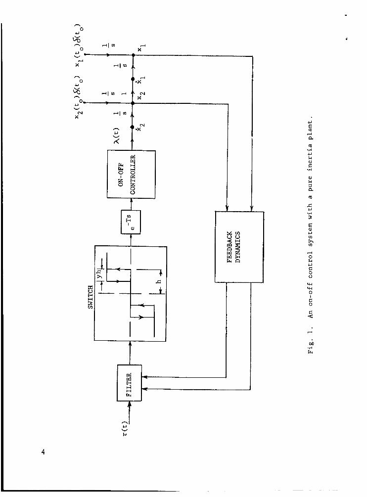
Consider the block diagram of a system shown in Figure 1. The

controlled element is a second order pure inertia plant whose output

position and output rate are represented by x and x2, respectively.

It is assumed that the switch has dead space such that the loop transient

always dies out before the application of control effort, , to plant

input.

1

Very often the dead space is deliberately introduced to avoid

erratic switching caused by random noise. The switch may also possess

hysteresis.

In a physical system there is a time delay, 7 , between switch- R

'YF , on and the application of control effort.

exists between switch-off and cut-off of control effort. This phenomena

is represented by the "delay" block in the figure. Notice that

and

into the system to obtain the desired switching characteristic and to

reduce noise effect. The filter can be either linear or nonlinear.

Systensof this type may appear as the stability subsystem or

Similarly, a time delay,

7R

TF are, in general, not equal. The "filter" block is inserted

reaction subsystem of a spacecraft cormnand module. The pure inertia

plant may represent a spacecraft traveling outside the earth atmosphere.

The rate diagram is a plot of the system rate at control removal

(xZf) versus the rate at control application (x~~).

transient dies out before control application, the output rate at

Since the loop

3

h

u 0

W

X"

t

U c m -I a m

*I4 U k aJ c -I4

a, k 3 a m

5 .rl 3

0 k c) G 0 L)

t: 0

c 4

4

M -4 Frc

4

control removal can be expressed as a function of control application.

If output amplitude characteristics of the switch and of the controller

I have odd symmetry with respect to their inputs, the rate diagram is also

symmetrical with respect to the origin. Therefore, it is sufficient to

consider only positive x and determine the values of x 2i 2f relative to

x2$ *

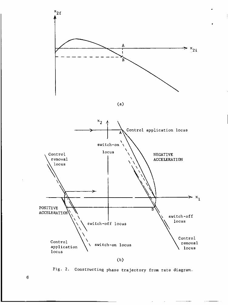
The system stability, transient response, and limit cycle behavior

can be analyzed via rate diagrams. Phase plane trajectories can readill

be constructed from the rate -am, and vice versa. Figure 2 illustrates

how to construct the phase plane trajectory from the rate diagram. Fig.

2a represents a rate diagram of a typical system and Fig. 2b is the phase

plane. Draw the control application line on phase plane, which is a

function of x and x only. Before control application the system

output coasts at a constant rate until it reaches the control application

1 2

line at A . Starting from A the system follows a constant acceleration

trajectory until it reaches B. Point B is the point where the control

is removed from the plant input. This point is given directly from the

corresponding B point on the rate diagram. Starting from B the system

again coasts at constant rate until it reaches the controller application

line on the opposite side.

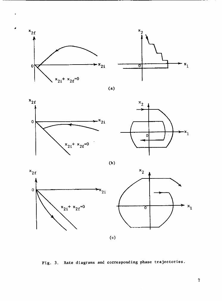
The behavior of the on-off system can be studied with the aid of

the rate diagram. When the rate curve lies in the first quadrant of the

rate plane, a stepping action occurs (Fig. 3a). That is, the phase

trajectory, which alternates between free coasting and constant acceler-

5

x2 f

Control application locus --r-pR switch-on ' \ \\

IEGATIVE

locus v , \ i i ~ ~ ~ ~ ~ ~ ~ ~ ~ ~ 1

ontrol application locus

ACCELERATION

1

ACCELE RATIO switch-of f

\ switch-on locus

(b )

F i g . 2. Constructing phase trajectory from rate diagram.

6

2f x2 X

2f X

0

2f X

x2 4

x2 4

1

Fig . 3 . Rate diagrams and corresponding phase t r a j e c t o r i e s .

7

ation, has a step pattern on phase plane. Under this cond

system eventually converges to a stable limit cycle. When

curve lies between the x -axis and the line x 4- X2f = 0 2i 2i

tion the

the rate

the system

output is oscillatory but conver.ges toward a stable limit cycle (Fig. 3G,

page 7 ) . If the rate curve lies between the x -axis and the line

x2it x~~

recrosses the x 4- x 0 line as x increases, the system would be

unstable.

2f

0, the system rate is divergent. And, unless the rate curve

2i 2f 2i

For most cases, the rate curve will intersect the line: x + 2i

An intersection indicates the existance of a limit cycle, x

since x = -x at such a point.

= 0 . 2f

2f 2i

The vector-state differential equations f o r the state variables

of the controlled element are:

In state-vector notation, the above equation may be rewritten:

where:

A = [ : :] and

( 3 )

( 4 )

8

The vector state differential equation may be solved by any of several

methods. 3y4y5 b

For the case where the input of the controlled element is

of the form: Act) = h a constant, the solution is:

For the derivation of the rate diagram equations, consider r(t) =

0. This defines an equilibrium state: - x =: 0. Thus, the response from

any initial state x(t ) will be defined. 0 -

From the preceding discussian, it is clearly seen that much

information is contained in a race diagram. The advantages of the rate

diagram over phase plane methods are obvious: (1) the rate diagram

curve considers all non-zero values of initial system rate on one plot.

This would be impractical for phase plane plots, (2) The effects of

changes in the values of the system parameters are shown directly. This

can often be difficult to surmise using phase plane techniques. ( 3 ) The

rate curves of different system cmfigurations can be shown on one plot

in order to compare the characteristics of the different configurations.

.This would be virtually impossible t o do using phase plane methods

without a resulting mesh of trajectories, thus making it difficult to

obtain meaningful information.

9

CHAPTER I11

RATE DIAGRAM ANALYSIS OF ON-OFF SYSTEM 1

DERIVATION OF EQUATIONS

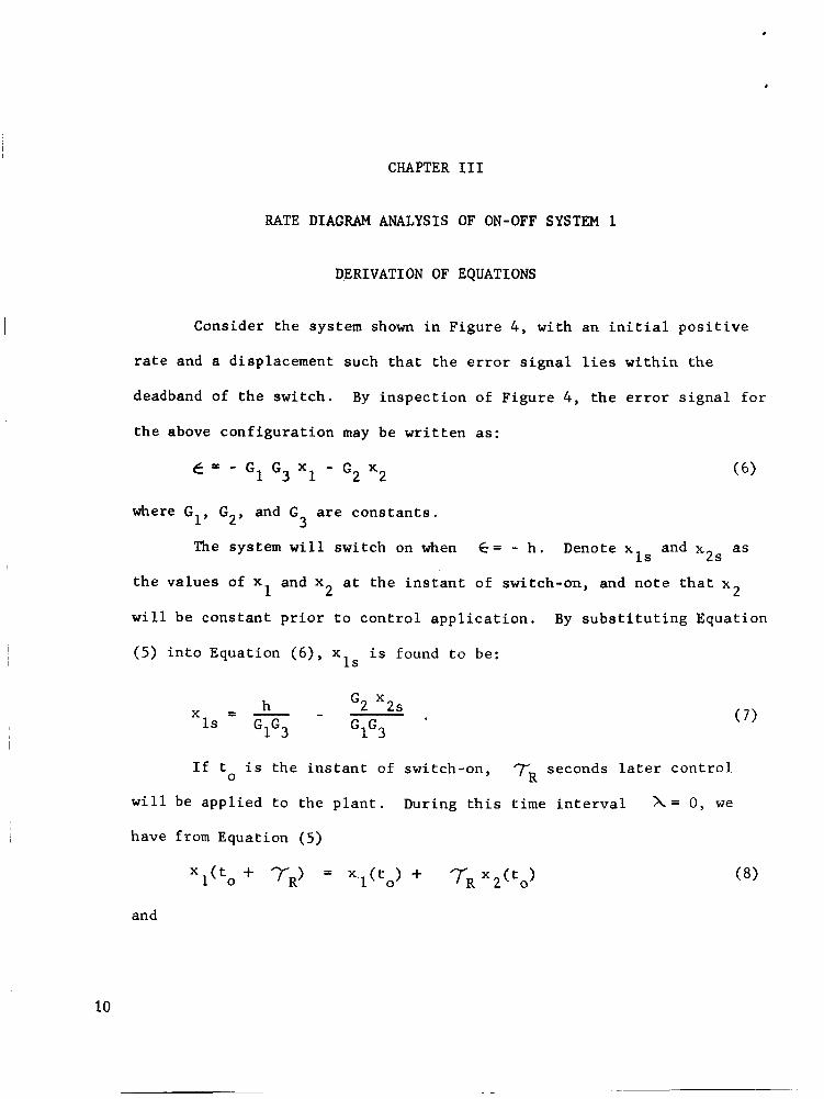
Consider the system shown in Figure 4 , with an initial positive

rate and a displacement such that the error signal lies within the

deadband of the switch.

the above configuration may be written as:

By inspection of Figure 4 , the error signal for

e = - G1 Gg X1 - G x 2 2

where G1, G2, and G are constants. 3

The system will switch on when e= - h. Denote x and x as 1s 2s

2 the values of x and x at the instant of switch-on, and note that x

will be constant prior to control application.

(5) into Equation ( 6 ) , x is found to be:

1 2

By substituting Equation

1s

x = - h - G 2 x 2 s

1s G1G3 G1G3

If t is the instant of switch-on, rR seconds later control A = 0 , we

0

will be applied to the plant.

have from Equation (5)

During this time interval

(7)

and

10

.

X

t I

E a,

11

I f t = 0 i s chosen as t h e time i n s t a n t of c o n t r o l a p p l i c a t i o n ,

then by s u b s t i t u t i n g Equat ion (5 ) i n t o (6 ) t h e e r r o r may be expressed as

A t 2 e ( t ) = - G l G 3 X l i - G G X . t f. G G -- 1 3 2 1 1 3 2

- G X 4- G 2 A t . (101 2 2 i

The sys tem w i l l switch-off when f = -h .f yh . Define t a s t h e i n t e r v a l

between t h e beginning of c o n t r o l a p p l i c a t i o n and s w i t c h - o f f .

1

Us19 t h i s

c o n d i t i o n i n Equat ion ( l o ) , t i s found t o be 1

- B1 4- B: - 4A1C1 t = 1 2A1

where

- G1G3 A1 - 2

B1 = G 2 ' r \ - G G x 1 3 2 i

C1 = h - G G x - G x - yh 1 3 li 2 2 i

rF seconds a f t e r s w i t c h - o f f , c o n t r o l i s removed from t h e p l a n t .

Denote x and x a s t h e v a l u e s of x anti x a t c o n t r o l removal. Using If 2 f 1 2

Equation (5)

12

The rate diagram for this systemmay now be constructed by

computing and plotting values of X for arbitrary values of X using

Equations (ll), (12) and the second one of (13).

2f 2i

THE RATE DIAGRAMS

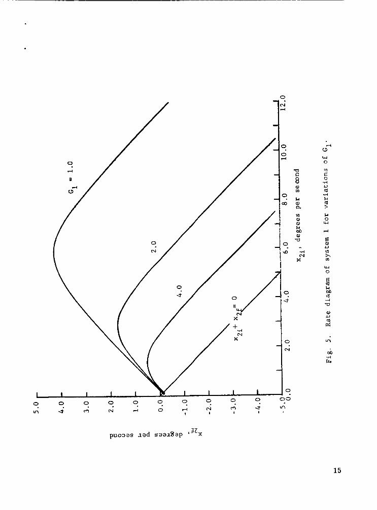
The nominal values of system parameters used for constructing

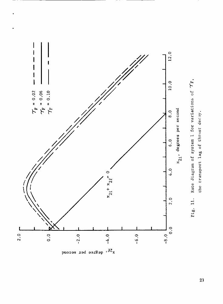
the diagrams are listed in Table I. Figures 5 to 11 are rate diagrams

for various system parameters.

REMARKS

The rate diagrams for System 1 show that the system is stable

for the values of system parameters considered. In addition, they

indicate that an "over-shooting" response results from large values of

initial rate, and a "stepping" response results from small values of

initial rate.

The limit cycle rate is affected as follows:

1. The limit cycle rate increases as G increases.

2. The limit cycle rate decreases as G2 increases.

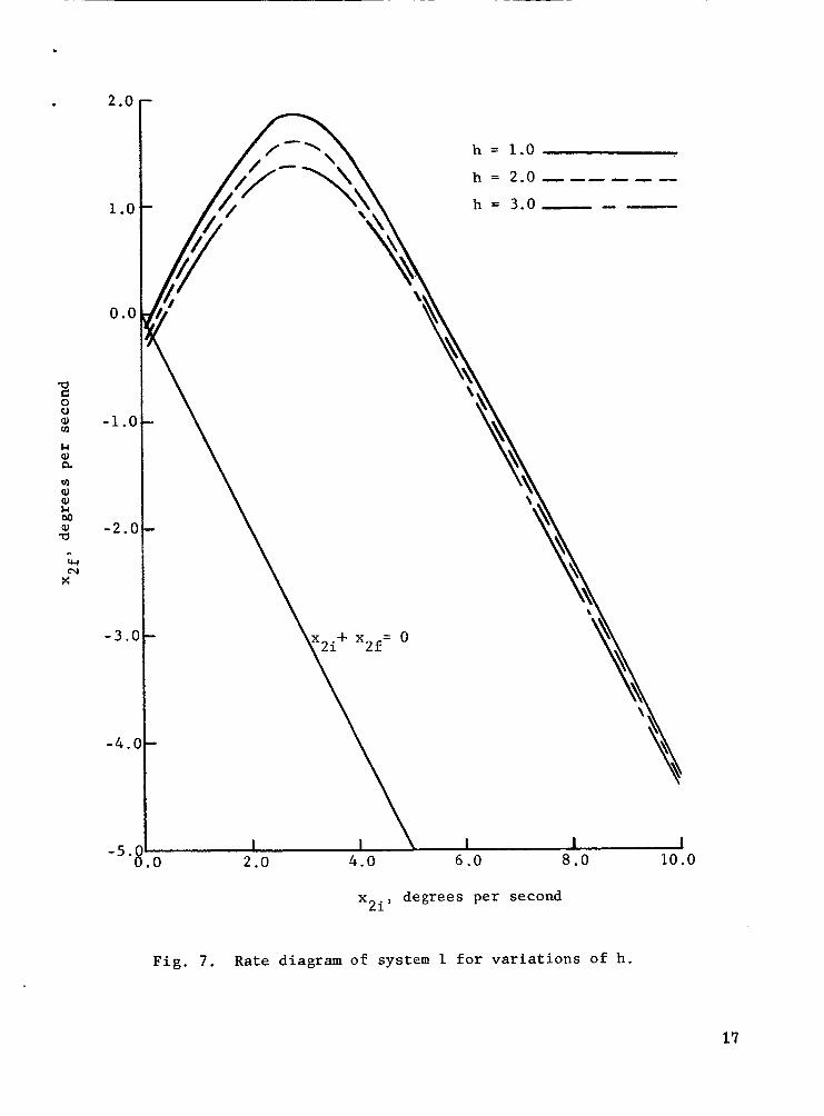
3. The limit cycle rate increases as h increases.

4 . The limit cycle rate increases as y increases.

5, The limit cycle rate increases as increases.

1

1

13

TABLE I

NOMINAL VALUES OF SYSTEM PARAMETERS FOR SYSTEM 1

Parameter Nominal Value Units

G1

G2

G3 h

Y

x 7 R

2.0

1 .o 1 .o

2 .o

0.05

ND

Degree-sec./degree

ND

Degrees

ND

6 . 0

0.02

0.02

L Degreeslsec.

Seconds

Seconds

14

l o / I - /

” /

/

o /

X

I I I I I I I 1 I 0 0 0

4. m CJ 4 0 m I I I I

0 0 4

0 cr)

0 e4

0 0 rc

0

a E:

a, rn

$4 a, a v1 a, a, & bo aJ a

8

* -?I N

X

puoDas l a d saax%ap c f L ~

15

puo3as l a d s a a i z a p c32x

16

-a C 0 u a, VI

& e, a VI aJ a, b bo a, a -

*rl hl

X

2 . 0

1 .o

0 .o

a c 0 0

m k al a m al a, k M

a

-1.0

a, -2.0 .. w

x"

- 3 . c

-5.1

h = 1.0

h = 2.0 - -- - - - h = 3.0- - -

x degrees per second 2 i '

F i g . 7 . Rate diagram of system 1 for variat ions of h .

17

a C 0 0 aJ m

& aJ a m aJ aJ l-l M aJ a I

w x-

2.0

1 .o

0.0

-1 .o

-2.0

-3.0

-4.0

- 5 . 0 0 .o

y =.o 2-----

y = . O 6 y =.l 0 --

x + x 2 f = 0 2 i

2.0 4.0 6.0 8 . 0

x , degrees p e r second 2 i

10.0

F i g . 8 . Rate Diagram of System 1 f o r v a r i a t i o n s o f y .

18

0

-0 c 0 c) aJ rn

Fc aJ a rn 0) aJ t-l M aJ -0 ..

-d N

x

C 0 -4 u (D

L-l 0 w rl

E aJ

/ + I

0 0 0

N 0 N I

puo3,as l a d s a a i s a p G32x

0 0

4 1

19

! I I ‘ I ‘ I

m - 0 0 0 4 . . .

/

0

hl

0 0

0 hl I

0 0

I

0

N 4

0

0 4

0

03

0

CD

0

4

0

hl

0

0 0

\o co I I

a c 0 CJ a, m

& a) a a, a, Ll M a, a .. *rl rJ

x

puosas l a d s?>r%ap ‘ 3 z ~

20

I I

1 I I

‘ I

0 c\1 I

0

0

N X

+ -I4

x-

0 0

I

0

N 4

0

0 rl

0

co

0

\D

0

d

0 N

0

0 0

a0 I

a c 0 u a, v)

$4 cu a m cu a, $4 M cu a .. 4 N

X

puoDas lad aai8ap c3zx

21

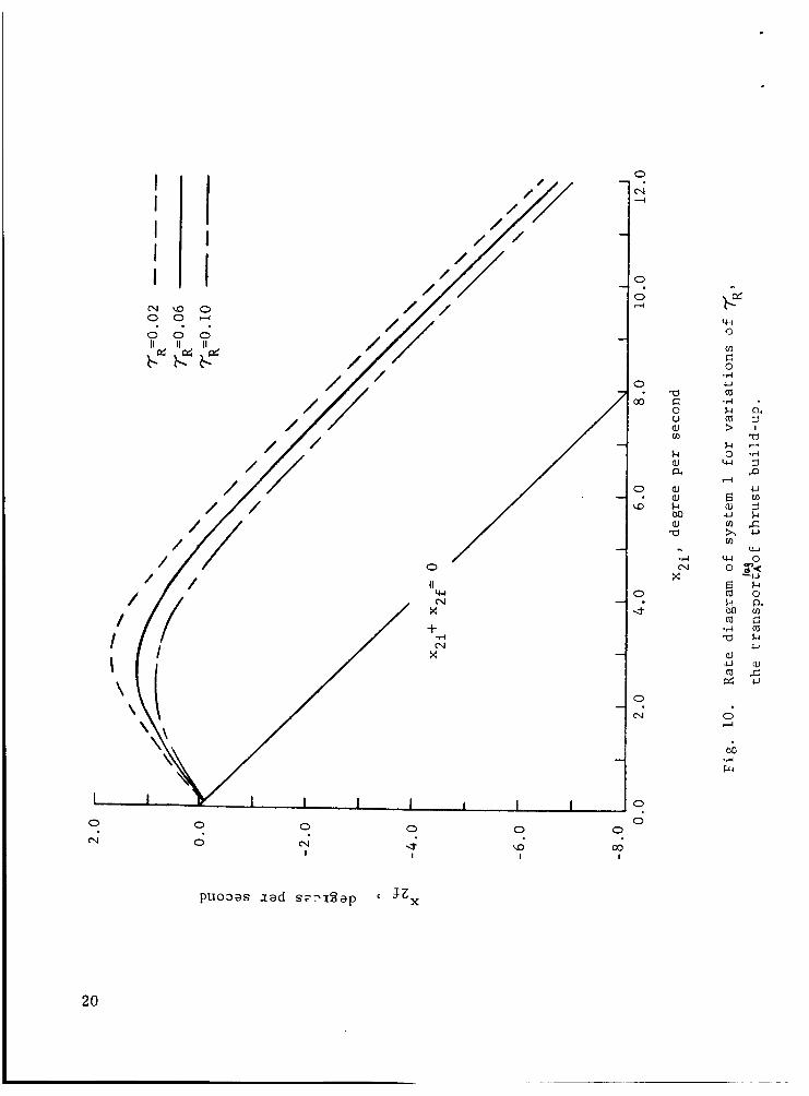
6. The limit cycle rate is independent of 7

7. The limit cycle rate increases as 7 increases. R '

F

22

CHAPTER IV

RATE DIAGRAM ANALYSIS OF ON-OFF SYSTEM 2

DERIVATION OF EQUATIONS

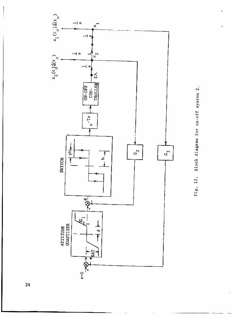
Consider the system shown in Figure 12 with an initial positive

rate and a displacement such that the errar signal lies within the

deadband of the switch. It will be necessary to classify the magnitude

of x in order to determine the correct error signal mode. 2i

I. h

By inspection of Figure 12, the error signal mode for this

magnitude of x is given by: 2i

E = - G x + G1(-G3 x1 + d) 2 2

The system will switch on when € = - h . Denoting the value of x and x at switch-on as x (t ) and x (t ) 1 2 1 0 2 0

respectively, the expression for x (t ) may be obtained by substituting

the above boundary condition into Equation (14) to yield:

2 2 0

1 0

- G x(t)+h +Gld (15) x(t)=

G1G3 1 0

Control will be applied to the system7 seconds after switch-on R

occurs. Denoting the values of x and x at the beginning of control 1 2

application as x and x and by utilizing Equation (S), the following li 2i'

expressions are obtained:

23

c 1c-l h f

l a

1

0

E a, u m h m

24

I [:‘i] 2i = [ x2(to>

= xl(to) + x2(to) 7R

SAT a Determine the value of time at which G ( - G x + d) = - e

1 3 1 When control‘ is applied to the ESAT * Define this value of time as t

system, x is given by the expression below. 1’

Xl(t) = x + x .t - - t2 (17) li 21 2

is found to be: ESAT Applying the given boundary conditions, t

- - -BESAT 7/8ESA; - %SAT ‘ESAT

%SAT ESAT t

where

- - G1G3 %SAT 2

= - G G x B~~~~ 1 3 2i

= - ( G G Y - G 1 d - e ) ‘ESAT 1 3 li SAT

It should be noted that the choice of sign for the radical is

determined by using the sign which results‘ in the smallest positive

It should also be noted that if the solution has real value of t

a complex value, then clearly, the stated boundary conditions will not

ESAT *

be attained by the system for the given initial conditions. This

procedure will be observed in the remainder of this anadysis whenever

there exists a possibility that the error signal does not saturate the

attitude quantizer.

25

Define: ?= G1(-G 3 1 x + d) (20) ’

Expanding the expression for yields:

2 7

t + G 1 d . (21)

G1G3 2 = - G G x - G G x t + p 1 3 li 1 3 2i

Differentiating the above expression and setting the result

equal to zero yields:

X

(22) 2i = -

tMAX h

where t

application and the instant at which the magnitude of p i s a maximum.

is defined as the interval between the beginning of control MAX

If tMAX

Define t

tESAT, then saturation does not occur.

as the interval between the beginning of control 1 application and switch-off. At switch-off,

= -h + yh .

Thus :

G 1 G 3 X 2 t + G 1 d

1 3 1 3 2i 1 2 1 - h + y h = - G G x l i - G G x t +

- G x + G 2 A t l . 2 2i

1 ’ Solving for t

- B1 2-B: - 4 AICl t = 1 A1

where:

26

.

B1 = G2h- - GlG3 x~~

I - C1 - - (G1G3 xli + G2 xZi + yh - h - G1 d) T seconds after switch-off, control is removed. F

saturation would occur. For this case, the > %SAT , If tMAx

analysis is continued as follows:

as shown below: ESAT' Evaluate x and x at time t = t 1 2

and the instant when ESAT Define t as the interval between t 2

switch-off occurs. During this interval,

e = - G x - e (28) 1 2 SAT '

Switch-off occurs when C = - h + yh. From the above information,

t is found to be: 2

) + y h - h eSAT -t- G2 X2(tESAT

G2 A t =

2

To investigate the possibility that switch-off does not occur

while the filter signal is saturated, the following procedure may be

used.

Define t as the interval between the beginning of saturation 5 and the end of saturation. The following equation is now applicable:

27

- - ) - G1G3 X2(tESAT) t5 - G G x ( t

SAT 1 3 1 ESAT - e

3

Solv ing f o r t, , J

5 t

where

A5

B5

c5

I f

o f f would

I f

I f

i n t e r v a l .

time l l o n I l

t

-B +7/B: - 4 A5 C5 - 5 - -

A5

- - G1G3 2

- - - G G x ( t ) 1 3 2 ESAT

t h e expres s ion f o r t

occur a t t h e end of t h e t i n t e r v a l .

t 5

t5

has a n e g a t i v e o r complex va lue , swi tch- 5

2

has a p o s i t i v e va lue , t h e fo l lowing procedure must be used .

t2, t h e system would swi tch o f f a t t h e end of t h e t 2

Cont ro l would be removed 7 seconds l a t e r . Thus, t h e t o t a l F

f o r a p p l i c a t i o n of c o n t r o l e f f o r t t o t h e system i s g iven by:

= t (33) -on ESAT + t 2 + t~

x may be eva lua ted a t t h i s t ime wi th r e s p e c t t o x u s i n g 2 i 2

Eqaution ( 5 ) , and t h e r a t e diagram may be c o n s t r u c t e d .

I f t5 < t 2 , t h e f i l t e r s i g n a l would o p e r a t e i n t h e l i n e a r mode

a g a i n , and t h e approach would be i d e n t i c a l t o t h a t used i n Equat ion (24)

with x and x a t t h e end of being r ep laced by t h e v a l u e s of x1 and x 2 li 2 i

28

, of the t interval. 5

In order for the switch to be off, the polarity and magnitude

of x must be such that the output of the attitude quantizer summed

with the rate feedback signal lies within the switching dead-band.

1

From inspection of Figure 6, 2i' Consider the case of positive x

page 16, the error signal mode for this magnitude of x is given by 2i

€ = - G x + G 1 ( - G x - d ) 2 2 3 1 (34)

The system will switch on when t = -h.

Denoting the value of x and x at switch-on as x (t ) and

x (t ) respectively, the expression for x (t ) may be obtained by

substituting the above boundary condition into Equation (34) to yield:

1 2 1 0

2 0 1 0

h - G2 X2(to) - G1 d x(t)=

G1G3 1 0 (35)

Control will be applied to the system 7 seconds after switch-on R occurs. Denoting the values of x and x at the beginning of control

application as x and x the following expressions are obtained:

1 2

li 2iy

Assume that the system will switch off while the error mode is

in the positive linear portion of the quantizer. In this mode, the

error signal is given by:

29

4 s - G x -I- G1(-G x - d ) (37) . 2 2 3 1

G1G3 2 - Gld (32 XZi + G2 At - G1G3 xli - G G x t + 2 = -

1 3 2i

(38)

The system will switch o f f when 6 = -h 4- yh . Define t as

the interval between the beginning of control application and switch-

off. Substituting the above boundary conditions into Equation (38)

yields:

1

- B - + -4r-Z 2A tl = (39)

where:

G1G3 A 2 A =

B = G 2 h - G G x 1 3 2i

C -(G1G3 xli + G2 xZi + G 1 d + y h - h )

Denote x and x as x (t ) and x (t ) . li 2i 1 0 2 0

Define t as the interval between t and the instant when dP 0

G1(-G3 x1 - d) = d .

Thus :

- B 2 7/B; - 4 A C t. =

2AP dP (43)

30

I where:

G1G3 2

B - GIGj x2(to) A = P

P

C -(G1G3 x(t) + G 1 d + d )

If tl < tdp, the assumption was correct. P

seconds later,

control is removed from the system.

(43)

However, if tl>t the assumption was incorrect. In this case, dP ’

, using Equation (5) tQ

evaluate x and x at the time t = 1 2

Define tdn as the interval between t and the instant when dP

- G x = - d . 3 1

Thus :

- B n k d B 2 n - 4 A n n C - - tdn 2An

where:

G3 A 2 A = n

31

Assume switch-off occurs during this interval. Note that during

( 4 9 ) this interval & = - G x 2 2‘

I I Switch-off would occur when e = -h + yh . Define t as the

1 interval between t and the instant of switch-off.

dP Substituting the given boundary conditions into Equation ( 4 9 ) ,

1 1

t is found to be: 1

I 1

If tl < tdn, then switch-off occurs during this interval. In

this event,

I 1

+

t = t 1 dP

where t 1 and switch-off.

is the interval between the beginning of control application

Control is removed from the system 7 seconds later. F

I I

If tl > tdn, switch-off would not have occurred during the For this case, the analysis may be continued as follows:

Evaluate x, and x at time t using Equation ( 5 ) .

interval.

2 dn ’ 1

32

as the interval between t and the instant when SATN dn Define t

SAT Gp(-G x + d) = - e 3 1

GlG3 t2 SATN Gld = - G G ~ ( t ) - G G ~ ( t ) tSAm+ SAT 1 3 1 dn 1 3 2 dn -e

may be solved from the following expression: SATN t

- B X k7/B2 X - 4 A C x x =

2AX SATN t

where:

GlG3 2 A =

X

BX = 'G1G3 X2(tdn)

SAT I C = - [ G1G3 xl(tdn) - Gld - e X

(54)

(55)

During this interval, the error signal is given by the following

expression:

G = - G x + G1(-G3 x1 + d) . 2 2

If switch-off occurs during this interval,

-h + yh = -G x (t ) + G 2 A t 3 - G G x (t ) - G G x (t )t 2 2 dn 1 3 1 dn 1 3 2 dn 3

+ Gld 3 G1G3 t + 2

(57)

where t is defined as the interval between t and the instant when

switch-off occurs. By solving the above equation, t is found to be: 3 dn

3

33

- B3 7/B: - 4 A3 C3

A3 t = 3

where:

Expanding the expression for )(, yields:

2 ~ 1 ~ 3 A t + G,d . (60) ? = -G1G3 Xl(tdn) - G1G3 X2(tdn>t + 2

Differentiating the above expression and setting the result equal

to zero yields:

is defined as the interval between t and the instant at MAX dn where t

which the magnitude of x is a maximum.

saturation does not occur. For this case, tSAT" If tW

t = t + t + t (62) 1 dp dn 3 *

Control would be removed from the system 7 seconds later. F

saturation would occur. The analysis may be > If tMAX

continued as follows:

Evaluate x and x at time t = t as shown below: 1 2 SATN '

34

and the instant when SATN Define t4 as the interval between t

switch-off occurs. During this interval,

e = - G x - e ( 6 4 ) 2 2 SAT *

Switch-off occurs when G = -h + yh . From the above information

t is found to be: 4

L

For the above case,

t = t + t 1 dp + tdn SATN + t4 .

F Note that in all cases, control is removed from the system T

seconds after switch-off. Evaluate x and x as the values of If 2f

Xl(tl + 7F) and x (t 2 1 F li + 7) with respect to x and x2i.

111. IG2 x2il> h + eSAT

In this mode, the system will be switched on independently of the

This may be easily verified as follows: lis value of x

Note that when the attitude quantizer is operating in the

saturation mode, the error signal is given by:

(67) SAT ' E = - G 2 x 2 + e

35

The system will be switched on when e = -h -h = -G x + e (68)

2 2 SAT

as the minimum positive value of x which results 2SAT 2i Define x

1' in the system switching on independently of the initial value of x

Thus, from Equation (68),

2SAT X

T R

X li

2i X

36

L

Q.E .D.

seconds after switch-on, control is applied to the system.

Define t as the interval between the beginning of control SAT

application and the instant when the attitude quantizer signal becomes

unsaturated. At this instant,

SAT G1(-G x - d) = e 3 1

Thus :

- A t2 - Gld . (72) - G1G3 x2i tSAT G1G3 2 SAT SAT 1 3 li = - G G x e

Therefore,

where:

(73)

x A~~~ = GiG3 T

( 7 4 )

Denote these as x (t ) and x2(tSAT) 1 2 SAT ' 1- SAT Evaluate x and x at t = t

respectively.

If I -G x (t SAT) + eSAT I >. h + yh , the system will still be

2i . In this case, denote x (t ) and x (t ) as x and x "on"

respectively, and follow the procedure outlined in Section 11, beginning

1 SAT 2 SAT li

with Equation (41), and adding t

"onll time . to the expressions for controller SAT

-G x (t < h + yh , the system has switched Although this is

If I 2 2 SAT

off before the quantizer signal becomes unsaturated.

unlikely, this condition is investigated as follows:

SAT = -G2 x2 + e

-h + yh = -G x 2 2i + G 2 X t~ + e~~~

theref ore,

SAT + y h - h - e G2 x2i t = G 2 x 1

TF seconds later, control is removed from the system.

THE RATE DIAGRAMS

(77)

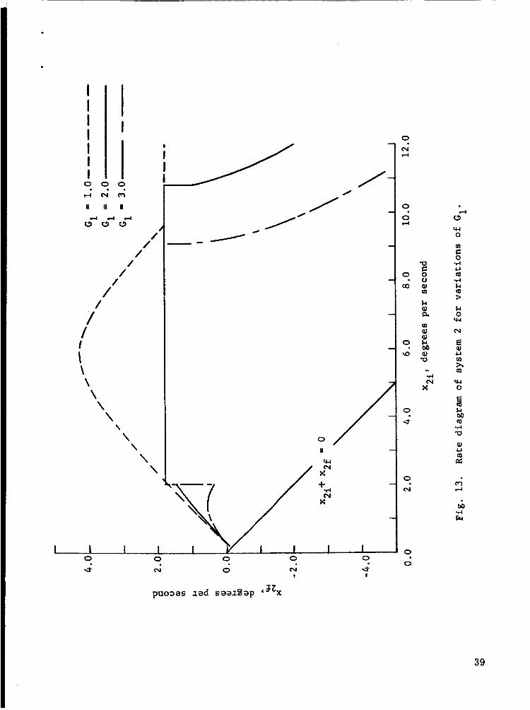
The nominal values of system parameters used for constructing the

rate diagrams are listed In Table 11. Figures 13-17 are the rate

37

TABLE I1

NOMINAL VALUES OF SYSTEM PARAMETERS FOR SYSTEM 2

Parameter Nominal Value Units

G1

d

SAT e

G 2

G3

h

Y

h

7 R

2 .o

2.5

15.0

1 .o

1 .o

2 .o

0.05

6.0

0.02

0.02

ND

Degrees

Degrees

Degree-sec./degree

ND

Degrees

ND

2 Degreeslsec.

Seconds

Seconds

I I I I I I I 0 4

II

x" +.d

t

N

II

0 m I

/

\ \ \ \

\ \

\ \ \ \

/ /'

0 II u.l /

0

4 0 N

0 0 0 N

t

0 4

I

0 N r(

0 0 I4

0 00

0

\o

0

4

0 N

0 0

a

0 al

g

k al a m aJ aJ #4 M 0) a ..

I4 0 W 0 ID

g

W 0

9 & M (d .A .. a a, U

2 m 4

M 4 F

puoaas l a d saaiaap 63zx

39

0 ' / II / / /

0

N

. . I / 1 II

0

" 0

0 0

" I

X

I I I I 0

4 I

0 \o I

0

N rl

0

0 rl

co

0

rD

0

0

N

0 0

03 I

a G 0 0 a, v)

&I a, a 0 a, a, f-l M a, a I

-4

X"

puo3as i a d saaifaap c3zx

40

eSAT= 5 . 0 ----- eSAT= 7 .5

eSAT= 10.0--- - -

a c 0 0 aJ

N aJ a rn aJ aJ k M aJ a

rn

.. ru

x"

2.1

0.

-2 .

-4.

- 6 .

-8.

-10.

0

\

\ \ \

\

I

2.0 4.0 8.0 10.0 12.0 0

x degrees per second 2i '

Fig . 15. Rate diagram of system 2 for variat ions of e SAT

41

42

k 0) a

4.0 c - - t / I

I I I

-8 .O t . I I I I I

0 .o 2.0 4.0 6 .O 8 .O 10.0 12.0

x degrees p e r second 2 i '

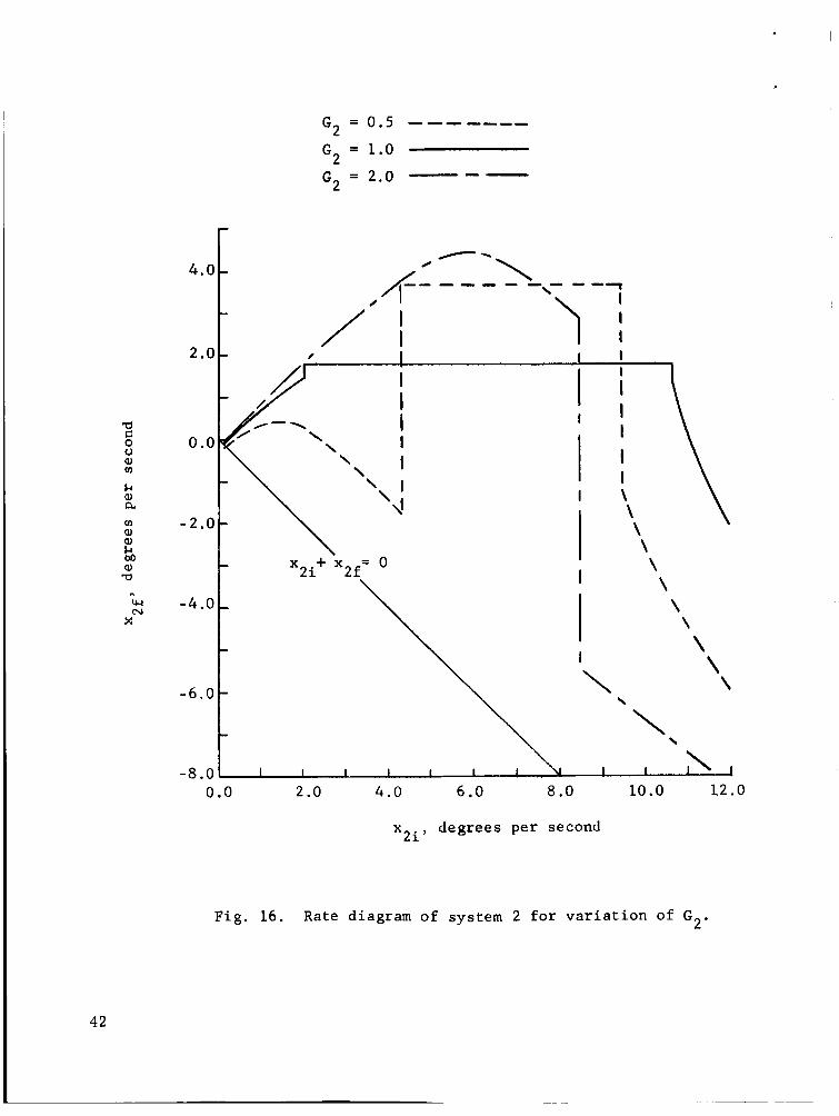
2 ' Fig . 16 . Rate diagram of system 2 f o r v a r i a t i o n of G

.

L I ---

.

0.0 p -2 .0

k r

-4.0

-6.0

0

\ \

\ \ \ \ \ I

G3 = O m 5 -- - -- -

G3

G3 = 1.0 = 2.0 - - -

I

x degrees per second 2 i '

0

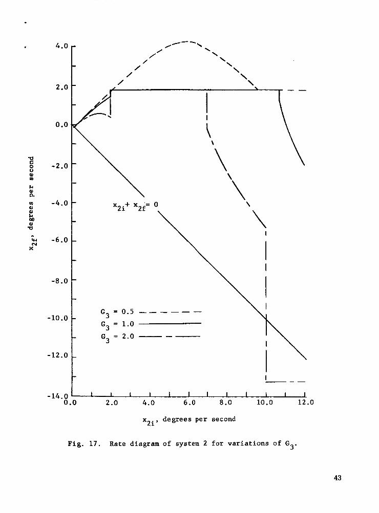
3' F i g . 1 7 . Rate diagram of system 2 for variations of G

43

diagrams for various system parameters.

REMARKS

The rate diagrams for System 2 indicate that a "stepping" response

results from a large range of values of initial rate. This type of

response is much faster than the "over-shooting" response. This

illustrates the improvements which may be obtained using a non-linear

filter for the error signal.

44

*

CONCLUSION

The use of rate diagrams f o r the design and eva lua t ion of a class

of on-off con t ro l systems has been i l l u s t r a t e d .

t h i s c l a s s of con t ro l systems would be an a t t i t u d e con t ro l system f o r a

space c r a f t opera t ing beyond an atmosphere.

an i d e a l s t e p func t ion i s a very good approximation t o the con t ro l torque.

It should be noted however, t h a t t he r a t e diagram i s not r e s t r i c t e d t o

systems us ing an i d e a l s t e p func t ion as the con t ro l ac t ion . For o t h e r

forms of con t ro l a c t i o n the equat ions become more complicated and i t may

be necessary t o resort t o numerical o r graphical methods t o solve the

e quat ions .

An important example of

For such systems, the u s e of

A suggested t o p i c f o r f u r t h e r research would be t o inves t iga t e

poss ib l e modif icat ions of the rate diagram concept t o include o the r

classes of on-off con t ro l systems.

4 5

REFERENCES

1, Patapoff, H., Rate Diagram Method of Analysis of an On-off Control - -7

System, AIEE Winter General Meetinz New York, N.Y., 1961.

2. Lake, R. C., Investigation of Transieqt and Limit Cycle Behavior of - the Stability Control Subsystem - the Apollo Command Module, FCA-63-6-17, LAD, North American Aviation, Inc., 1963.

Reaction Control Subsystem of

3. Hung, J. C., Unpublished - Class -’ Notes University of Tennessee, Winter Quarter, 1965.

4. Tou, J., Modern Control Theory, McGraw-Hill, New York, N. Y., 1964.

5. Rekoff, Jr., M. G., State Variable Techniques for Control Systems, Electro-Technology, New York, N. Y., May 1964.

47

.

A P P E N D I X 1

A PROGRAM T O D E T E R M I N E THE T R A N S I E N T RESPONSE OF ON-OFF CONTROL SYSTEM 1

C THE TRANSFER F U N C T I O N O F THE CONTROLLED E L E M E N T I S C O F THE FORM 1/S**20 C * * * * * C V A R I A B L E DESCR I P T I ON C G I FORWARD A T T I T U D E G A I N C G 2 R A T E FEEDBACK G A I N C C3 A T T I T U D E FEEDBACK G A I N C SWON CONTROLLER SW I TCH-ON THRESHOLD C PUHY S PER U N I T H Y S T E R E S I S O F S W I T C H C A C C E L ANGULAR A C C E L E R A T I O N L E V E L C TR TRANSPORT L A G F O R THRUST BUILD-UP C T F TRANSPORT L A G F O R THRUST DECAY C X I ANGULAR P O S I T I ON C x2 ANGULAR R A T E C * * * * * * c THE F O L L O W I N G V A L U E S O F SYSTEM PARAMETERS W I L L BE C C O N S I D E R E D NOMINAL. E A C H PARAMETER W I L L BE V A R I E D C S E P A R A T E L Y * WHILE THE OTHERS ARE HELD CONSTANT. C * * * * * *

GI = 200 G 2 = 1 0 0 G 3 = 1 0 0 SWON = 2 0 C P U H Y S = 0.05 ACCEL = 600 TR = 0002 T F = 0002

P R I N T 101

DO 1 K 1 = 50r400r25 FK1 = K 1 GI = FK1/1000 DO 2 I X = 2 0 r 1 2 0 0 r 2 0

X 2 I N = F L O A T X / 1000 C A L L SUB1 ( G l r G 2 r G 3 r SWONI PUHYSI A C C E L r T R r T F r

C * * * * * 101 F O R M A T ( 3 4 H G 1 W I L L BE V A R I E D FROM 0.5 T O 4.0)

3 F L O A T X = I X

1 X I I N I X ~ F I N I X ~ I N ~ X ~ F I N ~ TEEONE9 T I M E ) P R I N T l O O . G ~ r G 2 r G 3 r S W O N r P U H Y S , A C C E L I T R I T F I X I I N r

1 X I F I N ~ X ~ I N I X ~ F I N I T E E O N E I T I M E 2 CONT I NUE 1 CONT I NUE

G I = 200

*

*

49

102

7

1

1 6 5

C C

103

30

1

1 20 10

C C

1 0 4

7 0

1

1 60 50

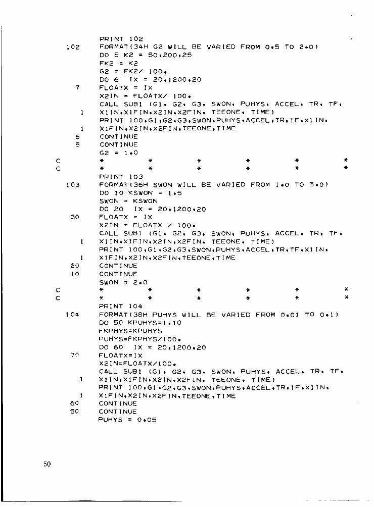
P R I N T 102 F.ORMAT(34l- l G 2 W I L L BE V A R I E D F R O M 005 T O 2 0 0 ) DO 5 K 2 = 50r200r25 F K 2 = K 2 G 2 = FK2/ 1000 DO 6 I X = 2091200920 F L O A T X = I X X 2 I N = F L O A T X I 1000 C A L L SUBl ( G l r C 2 r G 3 r SWONI P U H Y S r A C C E L r TR9 TFI X 1 I N r X l F I N r X 2 I N r X 2 F I N * T E E O N E 9 T I M E ) P R I N T l O O ~ G l r G 2 ~ G 3 r S W O N ~ P U H Y S I A C C E L t T R I T F I X l I N ~ XlFINrX2INrX2FINrTEEONErTIME CONT I NUE CONT I NUE G 2 = 1.0 * * * * * * * * * * * * P R I N T 103 F O R M A T ( 3 6 H SWON WILL BE V A R I E D FROM 100 TO 5 . 0 ) DO 10 KSWON = 1 9 5 SWON = KSWON DO 20 I X = 20r1200r20 F L O A T X = I X X 2 I N = F L O A T X / 1000 C A L L SUBl ( G l r G 2 r G 3 r SWONr P U H Y S r A C C E L r T R r T F I X I I N 9 X l F I N r X 2 I N r X 2 F I N r T E E O N E r T I M E ) P R I N T 100rGl~G2rG3rSWONrPUHYSrACCEL~TRrTF~XlIN~ XlFINrX2INrX2FINrTEEONErTIME CONT I NUE CONT I NUE SWON = 200 * * * * * * * * * * * * P R I N T 104 F O R M A T ( 3 8 H P U H Y S W I L L BE V A R I E D FROM 0.01 T O 0.1) DO 50 K P U H Y S = l r l O F K P H Y S = K P U H Y S P U H Y S = F K P H Y S / 1 0 0 0 DO 60 I X = 20r1200r20 F L O A T X = I X X 2 I N = F L O A T X / 1 0 0 . C A L L SUBl ( G l r G 2 r ’ G 3 r SWONr P U H Y S r A C C E L I T R * T F * X I I N I X ~ F I N * X ~ I N ~ X ~ F I N ~ T E E O N E 9 T I M E ) P R I N T lOOrGl*G2rG3rSWONrPUHYSrACCELrTRrTFrXlIN* X ~ F I N I X ~ I N ~ X ~ F I N ~ T E E O N E , T I M E CONT I NUE C O N T I N U E P U H Y S 0005

50

105

300

1

1 200 150

C C

106

700

1

1 600 500

107

35

1

1 25 15

c

PRINT 105 F O R M A T ( 3 B H A C C E L W I L L 8E V A R I E D F R O M 400 T O 1200) DO 150 K A C C E L = 4 * 1 2 * 2 A C C E L z K A C C E L DO 200 I X = 20r1200r20 F L O A T X = I X X Z I N = F L O A T X / l O O o C A L L SUBl (Glr G 2 r G3r SWONI P U H Y S r A C C E L r TRI T F r X l I N r X I F I N r X 2 I N ~ X 2 F I N r TEEONE. T I M E ) PRINT 1 0 0 r G l r G 2 t G 3 r S W O N ~ P U H Y S I A C C E L , T R I T F , X I I N ~ X1FINrX2fN*X2FINrTEEONErTIME CONT I NUE CONT I NU€ A C C E L = 6.0 * * * * * * * * * * * * PRINT 106 F O R M A T ( 3 5 H TR W I L L BE V A R I E D F R O M 0001 T O 001) DO 500 K T R Z l r l O FTRoKTR T R = F T R / l O O o DO 600 I X = 20r1200r20 F L O A T X = I X X 2 1 N = F L O A T X / l O O o C A L L SUBl ( G l r G2, G3r SWONr P U H Y S r A C C E L r TRr T F r X l I N r X l F I N r X 2 I N * X 2 F I N r TEEONE9 T I M E ) PRINT 100rG1rG2rG3rSWONrPUHYS~ACCEL~TR~TFrXlIN~ XlFIN*X21NrX2FINrTEEONErTIME C O N T I N U E CONT I NUE TR 0002 * * * * * * * * * * PRINT 107 F O R M A T ( 3 5 H TF W I L L BE V A R I E D F R O M 0001 T O 001) DO 15 K T F = l * l O FTF=KTF TF=FTF/100o DO 25 I X = 20r1200920 F L O A T X = I X X 2 1 N = F t O A T X / l O O o C A L L SUB1 (Glr G 2 r G3r SWONr P U H Y S I ACCELr TRI TF. X l I N r X l F I N r X 2 1 N r X 2 F I N r TEEONE9 T I M E ) PRINT ~ O O ~ G ~ ~ G ~ * C ~ ~ S W O N I P U H Y S I A C C E L , T R , T F I X I I N ~ XlFINrX2INrX2FINrTEEONErTIME CONT I NUE CONT I NUE TF = 0002

* *

51

C * * * * * 100 F O R M A T ( 7 F l l o 6 / 7 F l l o 6 / / )

END m

I > * * * * * S I B F T C SUB1 c * * * * *

1 X l I N * X l F I N * X 2 I N ~ X 2 F I N ~ TEEONE9 T I M E ) C * * * * *

S U B R O U T I N E SUB1 ( G I r G 2 r G 3 r S W O N t P U H Y S I A C C E L I T R I T F I

XlIN=SWON/(Gl+'G3)-(G2*X21N)/(Gl*G3)+X2IN*TR

B = G 2 * A C C E L - G I * G 3 * X 2 I N C=- (G2*X2IN+Gl*G3*X1IN+PUHYS*SWON-SWON)

A=Gl *G3*ACCEL/2 .0

C TEEONE IS THE I N T E R V A L FROM T H E B E G I N N I N G OF C CONTROL A P P L I C A T I O N UNTIL SWITCH-OFF OCCURS.

TEEONE=( -B+SQFT ( B * * 2 - 4 o * A * C ) ) / ( 2 o * A ) T l ME=TEEONE+TF X ~ F I N = X ~ I N + T I M E * X ~ I N - T I M E * * ~ * A C C E L / ~ O O X 2 F I N = X 2 I N - A C C E L * T I M E

C T H E R A T E D I A G R A M IS CONSTRUCTED B Y P L O T T I N G X 2 F I N C VERSUS T H E G I V E N V A L U E O F X 2 I N o

RETURN END

SENTRY

*.

* *

*

52

A P P E N D I X I 1

A PROGRAM T O D E T E R M I N E T H E T R A N S I E N T RESPONSE O F ON-OFF CONTROL SYSTEM 2

C THE TRANSFER F U N C T I O N OF THE CONTROLLED E L E M E N T IS C O F THE FORM 1/S**20 C * * * * * * C VAR I A B L E DESCR I PT I ON C G 1 G A I N OF A T T I T U D E Q U A N T I Z E R C DEE DEADBAND O F A T T I T U D E Q U A N T I Z E R C E S A T S A T U R A T I O N L E V E L OF Q U A N T I Z E R C G 2 R A T E FEEDBACK G A I N C G3 A T T I T U D E FEEDBACK G A I N C SWON CONTROLLER SWITCH-ON THRESHOLD C P U H Y S P E R UNIT H Y S T E R E S I S OF S W I T C H C A C C E L ANGULAR A C C E L E R A T I O N L E V E L C TR 1 TRANSPORT L A G F O R THRUST BUILD-UP C TF 1 TRANSPORT L A G F O R THRUST DECAY C x1 ANGULAR P O S I T I O N L

C x2 ANGULAR R A T E C * * * * * * C THE F O L L O W I N G V A L U E S ( OF SYSTEM PARAMETERS W I L L SE C C O N S I D E R E D NOMINAL. S A C H PARAMETER W I L L BE V A R I E D C SEPARATELY* WHILE THE OTr lERS ARE HELD CONSTANT. C * * * * * *

G 1 ~ 2 . 0 DEEz2.5 € S A T = 150 0 G 2 = 1 0 O G 3 = 1 0 O SWONZE 00 PUHYS= 0 05 A C C E L = 6 o O T R 1 = 0 0 0 2 TF1=0002

C * * * * * I P R I N T 101

101 FORMAT(34 i - l G 1 W I L L BE V A R I E D FROM 0.5 TO 5.0) DO 1 K 1 = 50r500*50 F K l =K1 G l = F K L /lo00 DO 2 I X = 2*120*2

3 F L O A T X = I X X 2 1 N = F L O A T X / l O o I F ( G 2 + X 2 I N-SWON 1595 *6

5 C A L L S U B H l ( G l r D E E * E S A T * G 2 r G 3 r S W O N * P U H Y S * A C C E L * T R l * 1 T F l ~ X 1 I N ~ X 2 I N ~ X l F I N ~ X 2 F I N * O N T I M E )

GO TO 7

*

53

6

7

I oc 2 1

C

102

203

205

206

207

200 2 0 2 20 1

C

103

303

305

306

307

330 302

C A L L S U B G H l ( G I ~ D E E * E S A T ~ G 2 r C 3 t S W O N ~ P U H Y S I A C C E L ~ T R l *

P R I N T 1 0 0 ~ G l ~ D E E ~ E S A T ~ G 2 ~ G 3 ~ S ~ O N ~ P ~ H Y S ~ A C C E L ~ T R l ~ 1 T F l r X l I N ~ X 2 I N t X l F I N ~ X 2 F I N ~ O N T I M E )

1 T F l t X l I N ~ X 2 I N ~ X 1 F I N ~ X 2 F I N ~ O N T I M E F O R M A T ( 8 F l l o 6 / 7 F l l o 6 / / ) C O N T I NUE C O N T I N U E G 1 ~ 2 . 0

PRINT 102 F O R M A T ( 3 5 H DEE WILL BE V A R I E D FROM 0.0 TO 5 0 0 ) DO 201 KDEE = 0 * 5 0 0 r 1 0 0 F K D E E Z K D E E

* * * * *

D E E = F K D E E / l O O o DO 202 I X = 20r1200920 F L O A T X = I X X 2 I N = F L O A T X / l O O o IF(G2*X2IN-SWON)205r205~206 C A L L SUBHl ( G I ~ D E E I E S A T I G ~ * G ~ ~ S W O N * P U H Y S Q A C C E L ~ T R ~ *

1 T F l r X 1 I N ~ X 2 I N ~ X 1 F I N ~ X 2 F I N ~ O N T I M E ) GO TO 207 C A L L S U B G ~ l ( G l r D E E * E S A T * C 2 r G 3 r S W O N 1 P U H Y S I A C C E L * T R l *

1 T F l r X l I N ~ X 2 I N ~ X l F I N ~ X 2 F I N ~ O N T I M E ) P R I N T ~ O O * G ~ ~ D E E I E S A T ~ G ~ ~ G ~ ~ S W O N ~ P U H Y S * A C C E L * T R ~ *

1 T F l ~ X 1 I N ~ X 2 I N ~ X 1 F I N t X 2 F I N ~ O N T I M E F O R M A T ( 8 F A 1 . 6 / 7 F 1 1 . 6 / / ) C O N T I NUE C O N T I NUE DE E=2 5 * * * * * * P R I N T 103 F O R M A T ( 3 7 r l E S A T W I L L BE V A R I E D F R O M 5.0 T O 15.0) DO 301 K E S A T = 1 0 * 3 0 * 5 F E S A T = K E S A T E S A T = F E S A T / 2 DO 302 I X = 2 0 r 1 2 0 0 9 2 C

X 2 I N = F L O A T X / 1 0 0 * IF(G2*X21N-SWON)305r305*306 C A L L S U B H l ( G l r D E E ~ E S A T ~ G 2 r G 3 r S W O " Y S , A C C E L * T R l *

F L O A T X = I X

1 T F l r X 1 I N ~ X 2 I N ~ X 1 F I N ~ X 2 F I N ~ O N T I M E ) GO TO 307 C A L L S U B G H l ( G l r D E E * E S A T q G 2 r G 3 r S W O N I P U H Y S I A C C E L * T R l *

1 T F 1 ~ X 1 I N ~ X 2 I N ~ X 1 F I N ~ X 2 F I N ~ O N T I M E ) P R I N T 3009 G ~ * D E E I E S A T I G ~ * G ~ ~ S W O N I P U H Y S I A C C E L I T R ~ ~

1 T F I * X 1 1 N * X 2 I N ~ X l F I N ~ X 2 F I N I O N T I M E F o R M A T ( 8 F 1 1 0 6 / 7 F 1 1 .e//) C O N T I NUE

*

3 0 1 C O N T I N U E

54

ESAT' 15 0

PRINT 104

DO 401 K 2 = 50,400r50 FK2=K2 G 2 = F K 2 / 1 0 3 0 DO 402 I X = 20r1200r20

X 2 1 N = F L O A T X / 1 0 0 . IF ( G 2 * X 2 I .J-SWON I405 405 9406

- c * * * * * 104 F O R M A T ( 3 4 H G 2 W I L L BE V A R I E D FROM 0.5 T O 4.0

403 F L O A T X = I X

405 C A L L S U B H l ( G l * D E E * E S A T * G 2 , C 3 . S W O " Y S I A C C E L * T R 1 * 1 T F l r X l I N ~ X 2 1 N r X l F I N ~ X 2 F I N I O N T I M E )

GO TO 407 406 C A L L S U B G ~ l ( G I ~ D E E ~ E S A T ~ G 2 r C 3 r S W O " Y S I A C C E L ~ T R l ~

1 T F l r X ' . I N * X 2 I N * X l F I N * X 2 F I N I O N T I M E ) 407 PRINT 4001 GlrDEE*ESATrG2rG3rSWONrPUHYS*ACCELrTRl*

1 T F l r X l I N ~ X 2 I N ~ X l F I N ~ X 2 F I N I O N T I M E 400 F O R M A T ( 8 F 1 1 0 6 / 7 F l l o 6 / / ) 402 C O N T I N U E 401 C O N T I N U E

C 2 x 1 00

P R I N T 105

DO 501 K 3 = 50r400r50 FK3=K3 G 3 = F K 3 / 1 0 0 . DO 502 I X = 20r1200r20

X 2 1 N = F L O A T X / l O O o I F ( G 2 * X 2 I N - SWON) 505r505r506

C * * * * * 105 F O R M A T ( 3 4 H G3 W I L L BE V A R I E D FROM 0.5 TO 4.0)

503 F L O A T X = I X

505 C A L L S U B H l ( G l r D E E r E S A T * G 2 , G 3 . S W O " Y S I A C C E L * T R l * 1 TFlrXlINrX2IN~XIFIN~X2FIN~ONTIME)

GO TO 507 506 C A L L S U B G H l ( G ~ * D E E I E S A T I G ~ ~ G ~ * S W O " Y S I A C C E L I T R ~ ~

1 T F l ~ X l I N r X 2 I N ~ X l F I N ~ X 2 F I N ~ O N T I M E ) 507 PRINT 500. G l v D E E r E S A T r G 2 r G 3 r S W O N I P U H Y S I A C C E L I T R l r

1 T F 1 ~ X l f N ~ X 2 I N ~ X 1 F I N ~ X 2 F I N ~ O N T I M E 500 F O R M A T ( 8 F l l o 6 / 7 F l l r 6 ~ / ) 502 C O N T I N U E 501 C O N T I N U E

END G 3 = 1 0 O

C * * * * * * S I B F T C SUBHl C * * * * * *

S U B R O U T I N E SUBHI ( G ~ ~ D E E ~ E S A T I G ~ I G ~ ~ S W O N * ~ U H Y S * A C C E L 1 ~ T R l r T F 1 ~ X 1 I N ~ X 2 1 N ~ X l F I N , O N T I M E )

*

*

55

C C C

$.

C

C C

11

12

13

15

17 1 1 1

16 50 5 1

C

* * * * * * X l T O W I L L BE C O N S I D E R E D A S T H E V A L U E OF X I A T T H E I N S T A N T O F SWITCH-ON. X1TO=(-G2*XEIN+ShON+Gl*DEE)/(Gl*G3) X l I N I S D C F I N E D A S T H E V A L U E O F X 1 A T THE B E G I N N I N G

X I I N = X 1 TO+X2 I N * T R l D E F I N E T 1 A S T H E I N T E R V A L BETWEEN THE B E G I N N I N G O F CONTROL A P P L I C A T I O N AND SWITCH-OFF. A 1 = G I * G 3 * A C C E L / 2 .

O F CONTROL A P P L I C A T I O N

B l = G 2 * A C C E L - G l * G 3 * X 2 I N C l = - ( G I * G 3 * X I IN+G2*X2IN+PUHYS*SWON-Gl*DEE - SWON) TI=(-BltSQRT(B1**2-4**Al*Cl))/(2.*Al) A E S A T = G l * G 3 * A C C E L / 2 . B E S A T = - G l * G 3 * X 2 1 N C E S A T = - ( G l * G 3 * X I I N - E S A T - G l * D E E ) R A D = B E S A T * * 2 - 4 e * A E S A T * C E S A T I F ( R A D ) 5 0 t l l t l l T E S A T = ( - 5 E S A T - S Q R T ( R A D ) ) / ( 2 o * A E S A T ) I F ( T E S A T ) 1 2 9 1 3 r 1 3 T E S A T = ( - B E S A T + S Q R T ( R A D ) ) / ( 2 . + A E S A T ) I F ( T E S A T ) 5 0 r 1 3 * 1 3

I F ( T M A X - T E S A T ) 5 0 * 5 0 * 1 5 X l E S A T = XlIN+X2IN+TESAT-TESAT**2*ACCEL/2* X 2 E S A T = X 2 I N - T E S A T * A C C E L T 2 = ( - S W O N + S W O N * P U H Y S + E S A T + G 2 * X 2 E S A T ) / ( G 2 * A C C E L ) I F ( T 2 ) 1 7 ~ 1 6 9 1 6 P R I N T 1 1 1 F O R M A T ( 3 5 H A N A L Y S I S MUST UE C O N T I N U E D F U R T H E R ) O N T I M E = 0.0 GO TO 5 1 T I = T E S A T + T 2 O N T I M E = T l + T F l X1FIN=XIIN+X2IN*ONTIME-ONTIME**2~ACC~L/2* X 2 F I N = X 2 I N - A C C E L * O N T I M E R E T U R N END

TMAX = X 2 I N / A C C E L

* * * * * *

B I B F T C S U B G H l

C * * * * * * S U B R O U T I N L S U B G H l ( G l * D E E * E S A T * G 2 r G 3 r S W O " Y S I l A C C E L ~ T R ~ ~ T F l r X l I N r X 2 I N t X ~ F I N t X 2 F I N ~ O N T I M E ~

C * * * * * * C DEFINE X 2 S A T A S T H E M I N I M U M P O S I T I V E V A L U E OF X 2 I N C W H I C H RESLlLTS I N T H E S Y S T E M B E I N G S W I T C H E D O N C I N D E P E N D E N T L Y OF T H E I N I T I A L V A L U E OF X I .

56

XESAT=(SWON+ESAT) /GE I F ( X 2 I N - X 2 S A T 11 I 1 ( 2

2 X l T O t 000 C N O T E T H A T F O R T H I S EXAMPLEI X l T O WAS CHOSEN C A R B I T R A R I L Y .

C DEFINE T S A T A S THE I N T E R V A L BETWEEN THE B E G I N N I N G C O F CONTROL A P P L I C A T I O N AND THE I N S T A N T WHEN THE C A T T I T U D E Q U A N T I Z E R S I G N A L EECOMES UNSATURATED.

X l I N = X l T O + X 2 I N U T R l

A S A T = G l *G3*ACCEL/2 . S A T = - G l * G 3 * X 2 I N C S A T = -(GI*G3*XlIN+Gl+DEE+ESAT) R A D = B S A T * * 2 - 4o*ASAT*CSAT I F ( R A D ) 56157157

56 PRINT 222 222 FORMAT (18H T S A T IS UNDEFINED)

O N T I M E = 0.0

57

5a 59

3

5 C C

60 6

GO TO 51 T S A T = (-BSAT-SQRT(RAD))/(~O*ASAT) IF ( T S A T ) 5 8 , 5 9 1 5 9 T S A T = ( -BSAT+SQRT(RAD)) / (2o*ASAT) X l T S A T = X ~ I N + X ~ I N + T S A T - T S A T * * ~ * A C C E L / ~ D X 2 T S A T = X 2 I N - A C C E L * T S A T

ERTSAT=-G2*X2TSAT+ESAT I F ( A B S ( E R T S A T ) - SWOFF) 59616 T1 = (-SWON-ESAT+SWON*PUHYS+G2*X2IN)/(G2*ACCEL) T l I S THE T I M E FROM T H E B E G I N N I N G O F CONTROL A P P L I C A T I O N UNTIL S W I T C H OFF. I F ( T I ) 6*60*60 I F ( T I - T S A T ) 50,50r6 X l T O = X l T S A T X 2 T O = X 2 T S A T

SWOFF=SWON-SWON*PUHYS

GO TO 11

X l T O = X l I N X 2 T O = X 2 I N

1 X1IN=(-G2*X21N+SWON-Gl*DE€)/(Gl*G3)+X2IN*TRl

T S A T = O o O C DEFINE T I P A S THE I N T E R V A L BETWEEN TO AND SWITCH-OFF.

11 A 1 P = GI *G3*ACCEL/2 . B l P = G 2 * A C C E L - G l * G 3 * X 2 T O C1P=-(G1*G3*X1TO+G2*X2TO+G1*DEE+SWON*pUHYS

R A D = BlP**2 - 4 o * A l P * C l P T I P = (-B1P - S Q R T ( R A D ) ) / ( 2 * * A l P ) IF ( T l P ) 76,75975

76 T I P = ( -B lP + S Q R T t R A 0 ) ) / ( 2 . * A l P )

1 - SWON)

57

I

75 ACP = G1*[;3*ACCEL/2. BDP = - G!*G3*X2TO CDP = -(Gl*G3*XlTO+G2*X2TO+Gl*DEE+DE)

--. s T D P I S D E F I N E D A S THE I N T E R V A L BETWEEN TO AND T H E c I N S T A N T WdEN G l * ( - G 3 * X l - D E E ) = DEE.

R A D = B D P * * 2 - 4o*ADP*CDP I F ( R A D ) 1 8 9 1 9 9 1 9

18 T 1 = T S A T + T 1 P GO TO 53

I F CTDP) 20,21921 1 9 T D P = ( - B ~ P - S Q R T ( R A D ) ) / ( ~ O * P D P )

20 T D P .= ( - B D P + S Q R T ( R A D ) ) / ( 2 o * A D P ) I F ( T D P ) 1 8 9 2 1 9 2 ;

21 I F ( T 1 P * T D P ) 1 2 9 1 2 9 1 3 12 T 1 = T S A T + T 1 P

GO TO 50 13 X ~ T D P = X ~ T J + X ~ T O * T D P - T D P * * ~ * A C C E L / ~ O

X 2 T D P = X 2 T O - A C C E L * T D P 6 1 ADN=G3*AC‘EL/2

B D N = - G 3 * X 2 T D P CDN=- ( G 3 * X 1 TDP-DEE )

R A D = BDN**2 - 4o*cADN*CDN C D E F I N E T D N A S T H E I N T E R V A L BETWEEN T D P AND THE C I N S T A N T WHEN ( - G 3 * X l = - D E E ) .

I F ( R A D ) 1 2 2 9 2 3 9 2 3 1 2 2 T l P P = (G2*X2TDP+SWON*PuHYS-SWON)/(G2+ACCEL)

C DEFINE T l P P A S THE I N T E R V A L BETWEEN T D P AND THE C I N S T A N T WHEN S W I T C H - O F F OCCURS.

I F ( T l P P ) 66922922

GO T C 59

I F ( T D N ) 24925925

66 T 1 = T S A T + T D P

23 T D N = ( - B D N - S Q R T ( R ~ D ) ) / ( ~ O * ~ D N )

24 T D N = ( - B D N + S Q R T ( R A D ) ) / ’ ( 2 o * A @ N ) 25 T l P P ( G 2 * X 2 T D P + S W O N * P U H Y S - S W C N ) / ( G 2 * b C C E L )

IF ( T I P P I 1 5 r 1 2 3 r 1 2 3 1 2 3 I F ( T l P P - T D N ) 2 2 * 2 2 9 1 5 22 T 1 = T S A T + T D P + T l P P

15 X ~ T D N = X ~ T L I P + X ~ T D P * T D N - T D N * * ~ * A C C E L / ~ . GO TO 50

X 2 T D N = X 2 T D P - A C C E L * T D N C D E F I N E T 3 A S T H E I N T E R V A L d E T W E E N T D N AND T H E C I N S T A N T \rJ:+EN SW I TCH-OFF OCCURS.

A 3 = G I * G 3 * A C C E L / 2 . B 3 = G 2 * A C C E L - G l * G 3 * X 2 T D N C 3 = - ( G l * G 3 * X l T D N + G 2 + ~ ~ ~ ~ N + ~ ~ / ~ N * P U H Y S - S W O N - G l * ~ ~ ~ ) R A D = B3**2 - 4 o * A 3 * C 3

I F i T 3 ) 2 3 9 3 0 9 3 0 28 T 3 = ( -83 - S Q R T ( R A D ! ) / ( 2 . * A 3 )

58

29 T 3 = (-83 + S Q R T ( R A D ) ) / ( 2 o * A 3 ) GO TO 30

30 AN=GI*G3*ACCEL/2 . RN=-G l *G3*XZTDN CN=-(Gl*G3*XITDN-Gl*DEE-ESAT) R A D = BN**2 - 4o*AN*CN I F ( R A D ) 3 1 9 3 2 9 3 2

31 T l = T S A T + TDP + TDN + T 3 GO TO 50

I F ( T S A T N ) 33934934

I F ( T S A T N ) 31934934

I F (TMAX - T S A T N ) 3 1 9 3 1 9 1 7

32 T S A T N = (-EN - S Q R T ( R A D ! ) / ( Z o * A N )

33 T S A T N = (-BN + S Q R T I R A D ) ) / ( 2 o * A N )

34 TMAX = XZTDN/ACCEL

17 X2SATN=X2TDN-ACCEL*TSATN X l S A T N = X~TDN+X~TDN*TSATN-TSATN**~*ACCEL/~O

C DEFINE T 4 A S THE I N T E R V A L BETWEEN T S A T N AND T H E C I N S T A N T O F S W I T C H OFF.

T4=(ESAT+G2*X2SATN+SWON*PUHYS-SWON)/(G2*ACCEL) A 5 = C l * G 3 * A C C E L / 2 o 85 = - G l * G 3 * X 2 S A T N C5 = -(Gl*G3*XISATN-Gl*DEE-ESAT) R A D = B5**2 - 4 o * A 5 * C 5 I F ( R A D ) 41937937

I F ( T 5 ) 38-39-39 37 T 5 = ( - B ~ - S Q R T ( R A D ) ) / ( ~ O * A ~ )

38 T 5 = ( - B S + S O R T ( R A D ) ) / ( 2 . * A 5 ) 39 I F ( T 4 - T 5 ) 4 1 9 4 1 r 4 2 . 42 X 1 T 5 = X l S A T N + X ~ S A T N * T ~ - T ~ * * ~ * A C C E L / ~ O

X 2 T 5 = X 2 S A T N - TS*ACCEL A 6 = G l + G 3 * A C C E L / 2 o 86 = G 2 w A C C E L - G l * G 3 * X 2 T 5 C 5 = -(Gl*G3*XlT5+G2*X215+SWON*PUHYS-SWON-GI*~EE) R A D = B6**2 - 4 o * A 6 * C 6 T 6 = ( - B ~ - S Q R T ( R A D ) ) / ( ~ O * A ~ ) IF ( T 6 ) 43944944

43 T 6 = ( - B O + S Q R T ( R A D ) ) / ( 2 o * A 6 ) 44 A T D N = G1*G3*ACCEL/2o

BTDN = - G I * G 3 * X 2 T 5 C T D N = -(.il+G3*XlTS-Gl*DEE-DEE) R A D = B T D N * * 2 - 4o*ATDN*CTDN IF ( R A D ) 48-45945

I F (TDN2) 46r47947

47 IF ( T D N Z - T 6 ) 40r48+48

GO TO 50

45 TDN2 = ( - JTDN-SQRT(RAD) ) / (2 .+ATDN)

46 TDN2 = ( - S T C N + S Q R T ( R A D ) ) / ( 2 o * A T D N )

48 T 1 = TSAT+TDP+TDN+TSATN + T 5 + T 6

59

60

40 P R I N T 1 1 1 1 1 1 F O R M A T ( 3 5 H A N A L Y S I S MUST BE C O N T I N U E D F U R T H E R )

O N T I M E = 0.0 GO TO 51

41 T l=TSAT+TDP+TDN+TSATN+T4 50 O N T I M E = T l + T F I 5 1 X l F I N = X I I N + X 2 I N * O N T I M E - D N T I M E + U 2 * A C C E L / 2 .

X 2 F I N = X 2 I N - A C C E L * O N T I M E R E T U R N END

S E N T R Y S I R S Y S