Managed Volatility Strategies: Applications to Investment PolicyFREDERICK E. DOPFEL AND SUNDER R. RAMKUMAR
FREDERICK E. DOPFEL
is an independent researcher and former managing director at BlackRock in San Francisco, [email protected]
SUNDER R. RAMKUMAR
is a managing director at BlackRock in San Fran-cisco, [email protected]
Investors have experienced surprises about market volatility through the recent financial crisis and continue to face the risk that risk will change.1 How
should they respond? When investors experi-ence stressed-market episodes and heightened uncertainty about future economic regimes, should their portfolios stay the same, or should they periodically de-risk portfolios by reducing allocations to risky assets?
The notion of the policy portfolio, representing current best practices for insti-tutional investors, is to maintain a static strategic asset allocation (SAA) based on assumptions about long-run (equilibrium) asset-class returns and volatility. As market values f luctuate, institutional investors typi-cally rebalance their portfolio holdings back to the original SAA holding ranges. These practices neglect considerations of present volatility or expectations of future vola-tility regimes.2 Deviations from the SAA to exploit market opportunities, including vola-tility regimes, would ordinarily be deemed an active decision or tactical asset allocation (TAA), which requires skill to be success-ful.3 But in this instance, changes in asset allocation are intended to be based on rules, rather than skills, and with less-frequent shifts that are associated only with more extreme market conditions.
We propose that investors, in their investment policy decisions, acknowledge
that f inancial markets periodically transi-tion between normal-volatility regimes and high-volatility regimes, in which risky assets appear to have unusually high risk that does not fit long-run assumptions. Depending on the persistence of volatility regimes and the ability to forecast them, investors may wish to adapt their portfolios to account for observed changes in volatility and volatility forecasts. Economic logic suggests that an investor would be willing to give up some expected portfolio return if the portfolio’s risk were lowered. Such investors may decide to de-risk the portfolio during the high-volatility storm and re-risk once skies are clear. This dynamic investment policy, called managed volatility, seeks a rule for adjusting asset allocation to the best risk–return tradeoff based on market conditions, as opposed to depending on skill to obtain an excess return, as in a classic TAA approach. This article assesses whether or not a managed volatility approach has advantages over static strategic asset allocation through normal- and high-volatility regimes.
We begin with a brief example to show how an investor seeking to maximize expected utility should respond to changes in forecast volatility. Specifically, the economic response to higher volatility is to de-risk the portfolio, unless Sharpe ratios increase pro-portionally with volatility. The second sec-tion examines financial history, to establish definitions of normal- and high-volatility
28 MANAGED VOLATILITY STRATEGIES: APPLICATIONS TO INVESTMENT POLICY FALL 2013
regimes, as well as the record of market performance in those regimes. This analysis demonstrates the persistence of high-volatility regimes and shows how historical returns have varied across normal- and high-volatility regimes. Sharpe ratios have remained fairly constant (or decreased) with volatility, justifying an approach that de-risks for periods of high volatility, aside from the ability to forecast regimes beyond historical relationships. In the third section, this historical analysis is used to set up a multi-period dynamic model and test the perfor-mance of managed volatility strategies (dynamic SAA) versus static SAA policy. We consider four hypothetical investors—“Naive,” “Strategic,” “Managed Volatility,” and “Prophetic”—representing a spectrum of skill levels and static/dynamic approaches to asset allocation. The benefits of managed volatility, as illustrated by the four investors, are shown to depend on the investor’s ability to forecast transitions in volatility regimes. The final section summarizes our recommendations for a managed volatility approach to strategic asset allocation.
ECONOMIC RESPONSE TO HIGHER VOLATILITY
The investor’s objective is to maximize expected utility by selecting the mix of assets that optimizes the risk–return tradeoff.4 This could be a mix of 60% stocks and 40% bonds, 40% stocks and 60% bonds, or any other combination. Based on the investor’s risk aversion, the investor may target more or less risk, coinciding with more or less expected return. In fact, we can infer an investor’s risk tolerance from his or her preferred mix of risky and risk-free assets.
In Exhibit 1, case 1 depicts a simplified picture of portfolio choice. The capital market line illustrates the investor’s opportunity set in risk–return space; the set of parallel iso-utility curves each represent combina-tions of risk and return that are equally desirable, where higher curves represent greater utility. In our example, an investor initially selects a 50/50 blend of risk-free and risky assets, which is tangent to an iso-utility curve and is thus optimal. Suppose we experience a sudden increase in expected risk, doubling the risk of both the risky asset and the initial portfolio. This is an enormous increase in expected risk; we use it to simplify calcula-tions and for graphic purposes, without loss of gener-ality for smaller, more realistic changes. Assuming (for now) that expected returns are unchanged, the initial
E X H I B I T 1Investors Should De-Risk in High-Volatility Regimes, Unless Sharpe Ratios Increase Significantly
portfolio shifts rightward in risk–return space and lies within a revised, less attractive opportunity set (revised capital market line). This original portfolio is no longer optimal from an investor utility perspective. Economi-cally, the risky asset has become more costly for the investor; therefore, the investor desires to hold less of it. The investor will move leftward and down along the revised capital market line to a new portfolio. The new portfolio is depicted at a point of tangency with another iso-utility curve, which is more desirable than the orig-inal portfolio at higher risk. The investor’s response to higher volatility is not only to de-risk the portfolio, but also to decrease risk below the original portfolio’s risk (87.5% risk-free and 12.5% risky). In this hypothetical example, the resultant low-return portfolio assumes the same level of risk aversion (utility function) implied by the original portfolio, and also assumes that the higher volatility will persist.
Nothing dictates that expected returns will be constant in a higher-volatility regime. Exhibit 1, case 2 begins with the same portfolio. Expected risk increases, as in the previous example, but in the special case that expected Sharpe ratios (excess return/risk) are constant. In this case, the opportunity set is unchanged and the risk increase causes the initial portfolio to shift along the same opportunity set (original capital market line), resulting in more risk and proportionally more (excess) returns. However, the original portfolio is less preferred by the investor and no longer optimal from an investor utility perspective. As shown, the investor’s response to higher volatility is to de-risk the portfolio back to the original risk budget and return by halving the alloca-tion to risky assets (75% risk-free and 25% risky) in this hypothetical example.
We build a final example in which the investor desires to retain the original portfolio holdings in the face of higher volatility, as shown in case 3, with a doubling of expected risk and a proportional increase (doubling) of the expected Sharpe ratio (a bold assump-tion). The original portfolio is on a new opportunity set (revised capital-market line) that is tangent to a higher iso-utility curve, and thus optimal. In other words, risk doubles while the expected excess return quadruples. The investor responds by keeping the original portfolio holdings (50% risk-free and 50% risky). This property of constant holdings in the face of higher volatility hap-pens only when the increase in expected risk is matched by a proportional increase in expected Sharpe ratio.5
Any smaller increase in expected Sharpe ratio results in de-risking, back toward the original risk budget (if there is a less-than-proportional increase in the Sharpe ratio) or beyond to a lower-risk budget (if the Sharpe ratio declines). Although this scenario seems extreme in terms of its requirement of a proportional increase in expected Sharpe ratio, it is the simplest condition that justifies current practices of rebalancing portfolios back to the original SAA holdings.
These examples illustrate the motivating principles behind managed volatility, but they are highly simplified.6 We have assumed that an investor’s risk aversion, although unobservable, is constant over time as an approximation. Ever since the development of the intertemporal capital asset pricing model (Merton [1973]), financial econo-mists have tried to model how investors’ portfolio choices change over time according to expected returns, expected volatility, and changes in risk aversion. The debate about whether risk aversion may be procyclical or countercy-clical continues and is difficult to resolve, because the parameters underlying investor choice may be unobserv-able. The examples further assumed that changes in vola-tility were permanent, whereas they are more likely to be transitional, as demonstrated later in this article.
Nevertheless, the examples of economic response to higher volatility demonstrate that current practices for SAA and rebalancing have a major deficiency in ignoring volatility regimes. The examples also highlight the importance of defining volatility regimes clearly and describing the associated market response in terms of expected Sharpe ratios.
HISTORICAL VOLATILITY REGIMES
The viability of a managed volatility approach depends on the link between volatility and returns and the persistence of volatility regimes through time.7 We analyze historical data to answer three key questions:
1. Are there distinct volatility regimes with different risk/return characteristics?
2. Are these regimes persistent and predictable?3. How robust are the results across markets?
We begin by examining long-run data on the S&P 500. Volatility measurement depends on the investor’s time horizon, with smoother returns experienced over longer periods. In our analysis, however, we elect to focus
30 MANAGED VOLATILITY STRATEGIES: APPLICATIONS TO INVESTMENT POLICY FALL 2013
on a more responsive measure of volatility, because most investors—even those with long time horizons—care about outcomes over intermediate periods; that is, the journey matters. We analyze quarterly periods because this corresponds to the typical frequency of rebalancing and policy decisions, and we calculate a simple measure of annualized volatility, using daily return data within the quarter.8 This results in non-overlapping measures of volatility, as illustrated in Exhibit 2. The chart shows how dramatically volatility has varied through time, with periodic ebbs and f lows. The Great Depression stands out as a very unusual period of exceptionally high and sustained volatility, and the extreme nega-tive returns experienced then may exaggerate the link between volatility and returns. Therefore, we ignore this period in our base case and focus on the post-war period from 1950 to 2011. We also report full period statistics later in this section.
Having selected our sample period, we must define alternate volatility regimes. In principle, there may be a continuum of regimes, but we focus on just two states: a normal-volatility regime defined by moderate vola-tility and a high-volatility regime defined by outsize volatility. By analyzing two materially different states of the world, we not only keep the analysis simple and capture the problem’s essence, but we also avoid over-interpreting noise that may confound an analysis of very finely divided volatility periods. Because our analysis focuses on the effect of policy action in more extreme environments, we define the top 5% of quarters with the highest volatility as representing the high-volatility regime, and the remaining 95% of quarters as normal
volatility. This results in a volatility cutoff of 25.3%, with high-volatility periods illustrated by gray shaded bars in Exhibit 2.9 A 5% cutoff should imply high-volatility regimes that occur once every five years, or one in 20 quarters. On average, however, we saw such periods every 10 years in the post-war decades, followed by a clustering of high volatility during the credit crisis and its aftermath. A study of volatility regimes is thus particularly timely today, as many would predict con-tinued elevated volatility, given the uncertainty about the future economic environment.
We calculate regime characteristics in two ways: Ex post calculations are based on the realized volatility at the end of the quarter, while ex ante calculations are based on the forecast volatility at the beginning of the quarter (based on the previous quarter). Ex post results clearly illustrate the volatility’s concurrent effect on returns but assume perfect foresight in predicting quarterly vola-tility. In contrast, ex ante calculations only assume that we observe current volatility and let us study the impact of forecast error. Exhibit 3 illustrates the ex post distri-bution of regime returns in the post-war period, and the table describes statistics.10 The differences between regimes are stark. Normal realized volatility periods had positive excess returns on average, with fairly tight returns distribution. In contrast, high realized volatility periods yielded large negative average returns with much more dispersion, consistent with the elevated volatility. This difference between regimes is both statistically and economically significant, with a t-statistic of 4.7.
We repeat this exercise across a broad set of eight additional equity indices, as illustrated in Exhibit 4.11
E X H I B I T 2Volatility Has Varied Dramatically through Time, with Periodic Transitions between Normal and High Volatility
Sources: BlackRock and Standard & Poor’s, 1928–2011.
The indices include large-cap and small-cap segments, developed and emerging markets, as well as a set of indi-vidual country indices. In each case, as before, we define the 5% of quarters with the highest realized volatility as the high volatility regime and compute risk and return statistics. While the indices all have varying inception dates and varying thresholds that define high volatility, the impact on returns is remarkably similar. In all the cases, high realized volatility regimes were associated with negative average excess returns, greater dispersion, and significantly lower Sharpe ratios than normal real-ized volatility periods. The differences in Sharpe ratio were most extreme for the MSCI UK Index and least extreme for the MSCI Japan Index, where a part of the high-volatility regime coincided with strong stock market expansion in the late 1980s.
Our study so far highlights the relationship between returns and volatility regimes on an ex post basis. In reality, investors cannot identify regimes with perfect hindsight. Investors may observe the current regime (i.e., whether volatility is elevated or not) but must forecast the future regime. Their investment deci-
sions and returns thus depend on regimes’ persistence and predictability.
Exhibit 5 describes the regime transition probabili-ties and performance characteristics of volatility regimes for the S&P 500, based on quarterly data from 1950 to 2011. The chart illustrates four possible transitions: normal to normal, normal to high, high to normal, and high to high. Markets are in periods of persistent normal volatility (normal-normal) most of the time, by definition. These periods are typically associated with stable markets and have positive excess returns and low volatility. The transition to high volatility (normal-high) usually occurs during a market dislocation and is associ-ated with significant negative excess returns. This is the worst regime transition for the investor. In contrast, the transition from high to normal volatility (high-normal) is the most attractive regime transition. It is typically associated with improving sentiment and has the highest average excess returns. Finally, persistent high volatility (high-high) results in the greatest elevated volatility and has modestly negative average excess returns, likely driven by the continued uncertainty. Although the
E X H I B I T 3High Levels of Realized Volatility Have Been Associated with Negative Average Returns
Sources: BlackRock and Standard & Poor’s, 1950–2011. All results are annualized, based on monthly data.
32 MANAGED VOLATILITY STRATEGIES: APPLICATIONS TO INVESTMENT POLICY FALL 2013
transition outcomes are quite intuitive, the transition probabilities exhibit a surprising degree of persistence. The historical data show a 36% probability of a high-volatility quarter persisting, compared with 5% assuming
statistical independence (randomness), which is statistically signif icant at the 99% confidence level. Similarly, there is a 97% probability of a normal volatility persisting, compared with 95% assuming statistical independence.
Although regimes are relatively per-sistent, there is enough uncertainty about transitions to highlight the difference between ex ante returns (assuming we know only the current volatility regime and the transition probabilities) and the ex post returns previously reported (that presume perfect hindsight). The forward-looking (ex ante) expected returns in the normal volatility regime are a weighted expectation of moderate returns with a (high) probability of recurrence of normal volatility and severe negative returns with a (low) probability of transition to a high-volatility regime. Similarly, the expected
returns in high-volatility periods are a weighted expec-tation of negative returns associated with a 36% proba-bility of recurrence of high volatility and outsize positive returns with a 64% probability of transition to normal
E X H I B I T 5Although Returns Vary Significantly during Regime Transitions, Volatility Regimes Tend to Be Persistent
Sources: BlackRock and Standard & Poor’s, 1950–2011. All results are annualized, based on monthly data.
E X H I B I T 4The Inverse Relationship between Realized Volatility and Returns Is Consistent across Markets
Sources: BlackRock, Standard & Poor’s, Russell, and MSCI, as of 09/30/2012. All results are annualized, based on monthly data.
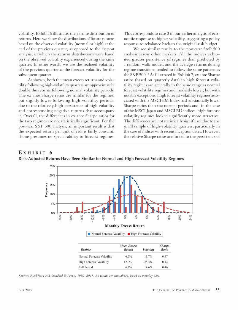
volatility. Exhibit 6 illustrates the ex ante distribution of returns. Here we show the distributions of future returns based on the observed volatility (normal or high) at the end of the previous quarter, as opposed to the ex post analysis, in which the returns distributions were based on the observed volatility experienced during the same quarter. In other words, we use the realized volatility of the previous quarter as the forecast volatility for the subsequent quarter.
As shown, both the mean excess returns and vola-tility following high-volatility quarters are approximately double the returns following normal volatility periods. The ex ante Sharpe ratios are similar for the regimes, but slightly lower following high-volatility periods, due to the relatively high persistence of high volatility and corresponding negative returns that accompany it. Overall, the differences in ex ante Sharpe ratios for the two regimes are not statistically significant. For the post-war S&P 500 analysis, an important result is that the expected return per unit of risk is fairly constant, if one presumes no special ability to forecast regimes.
This corresponds to case 2 in our earlier analysis of eco-nomic response to higher volatility, suggesting a policy response to rebalance back to the original risk budget.
We see similar results to the post-war S&P 500 analysis across other markets. All the indices exhib-ited greater persistence of regimes than predicted by a random walk model, and the average returns during regime transitions tended to follow the same pattern as the S&P 500.12 As illustrated in Exhibit 7, ex ante Sharpe ratios (based on quarterly data) in high forecast vola-tility regimes are generally in the same range as normal forecast volatility regimes and modestly lower, but with notable exceptions. High forecast volatility regimes asso-ciated with the MSCI EM Index had substantially lower Sharpe ratios than the normal periods and, in the case of the MSCI Japan and MSCI EU indices, high forecast volatility regimes looked significantly more attractive. The differences are not statistically significant due to the small sample of high-volatility quarters, particularly in the case of indices with recent inception dates. However, the relative Sharpe ratios are linked to the persistence of
E X H I B I T 6Risk-Adjusted Returns Have Been Similar for Normal and High Forecast Volatility Regimes
Sources: BlackRock and Standard & Poor’s, 1950–2011. All results are annualized, based on monthly data.
34 MANAGED VOLATILITY STRATEGIES: APPLICATIONS TO INVESTMENT POLICY FALL 2013
high volatility in the sample period. The MSCI EU and MSCI Japan indices exhibited the lowest historical per-sistence (25% and 13%, respectively) and the relatively large likelihood of moving back to the normal-volatility regime biased up the average return.
This ex ante analysis is the simplest type of forecast based on historical frequencies of state transitions. There are many ways in which investors can improve their forecasts of volatility regimes. This can range from using more recent data (e.g., monthly periods),13 to advanced forecasting models, to implied volatility (e.g., the VIX) and other predictors.14 Rather than prescribe volatility forecasting techniques, our emphasis is on policy rules for changing volatility and the question of whether a managed volatility approach has any merit. In the next section, we evaluate managed volatility using a simple regime model and contrast the performance of strategic investors with static holdings of risky assets to inves-tors with dynamic holdings based on varying degrees of forecasting skill.
POLICY RULES FOR VOLATILITY REGIMES
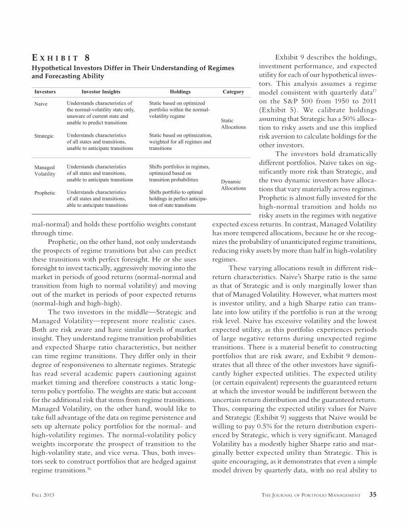
Investors may differ greatly in their understanding of market dynamics (historical volatility), their ability to forecast volatility regimes, and their approach to asset allocation policy, whether static or dynamic. In order to illustrate optimal policy rules, we consider four hypo-thetical investors: Naive, Strategic, Managed Volatility, and Prophetic,15 each with different levels of insight and static/dynamic orientation. Each investor has the same risk preferences and creates optimized portfolios based on world view and forecasting skill. Exhibit 8 describes the investor personalities and portfolio construction methodology.
Naive and Prophetic are at two extreme ends of the spectrum. Naive, as the name suggests, does not under-stand regime transitions, does not know what regime he or she is in, and always assumes that the market will remain in a normal volatility state. He or she constructs a fairly aggressive portfolio consistent with the attrac-tive characteristics of persistently normal regimes (nor-
E X H I B I T 7Across Markets, Sharpe Ratios in High Forecast Volatility Regimes Have Generally Been of the Same Magnitude as, or Lower than, Normal Forecast Volatility Regimes
Source: BlackRock, Standard & Poor’s, Russell, and MSCI, as of 12/2012. All results are annualized, based on monthly data. Asterisks imply 95% statistical significance.
mal-normal) and holds these portfolio weights constant through time.
Prophetic, on the other hand, not only understands the prospects of regime transitions but also can predict these transitions with perfect foresight. He or she uses foresight to invest tactically, aggressively moving into the market in periods of good returns (normal-normal and transition from high to normal volatility) and moving out of the market in periods of poor expected returns (normal-high and high-high).
The two investors in the middle—Strategic and Managed Volatility—represent more realistic cases. Both are risk aware and have similar levels of market insight. They understand regime transition probabilities and expected Sharpe ratio characteristics, but neither can time regime transitions. They differ only in their degree of responsiveness to alternate regimes. Strategic has read several academic papers cautioning against market timing and therefore constructs a static long-term policy portfolio. The weights are static but account for the additional risk that stems from regime transitions. Managed Volatility, on the other hand, would like to take full advantage of the data on regime persistence and sets up alternate policy portfolios for the normal- and high-volatility regimes. The normal-volatility policy weights incorporate the prospect of transition to the high-volatility state, and vice versa. Thus, both inves-tors seek to construct portfolios that are hedged against regime transitions.16
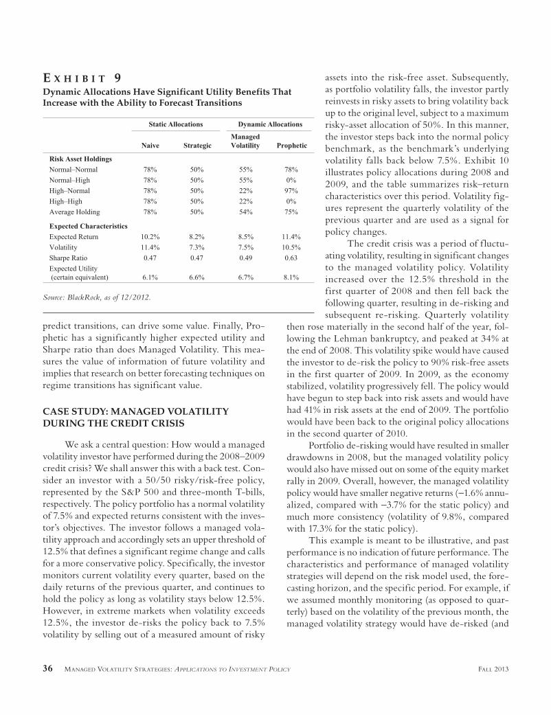
Exhibit 9 describes the holdings, investment performance, and expected utility for each of our hypothetical inves-tors. This analysis assumes a regime model consistent with quarterly data17 on the S&P 500 from 1950 to 2011 (Exhibit 5). We calibrate holdings assuming that Strategic has a 50% alloca-tion to risky assets and use this implied risk aversion to calculate holdings for the other investors.
The investors hold dramatically different portfolios. Naive takes on sig-nificantly more risk than Strategic, and the two dynamic investors have alloca-tions that vary materially across regimes. Prophetic is almost fully invested for the high-normal transition and holds no risky assets in the regimes with negative
expected excess returns. In contrast, Managed Volatility has more tempered allocations, because he or she recog-nizes the probability of unanticipated regime transitions, reducing risky assets by more than half in high-volatility regimes.
These varying allocations result in different risk–return characteristics. Naive’s Sharpe ratio is the same as that of Strategic and is only marginally lower than that of Managed Volatility. However, what matters most is investor utility, and a high Sharpe ratio can trans-late into low utility if the portfolio is run at the wrong risk level. Naive has excessive volatility and the lowest expected utility, as this portfolio experiences periods of large negative returns during unexpected regime transitions. There is a material benefit to constructing portfolios that are risk aware, and Exhibit 9 demon-strates that all three of the other investors have signifi-cantly higher expected utilities. The expected utility (or certain equivalent) represents the guaranteed return at which the investor would be indifferent between the uncertain return distribution and the guaranteed return. Thus, comparing the expected utility values for Naive and Strategic (Exhibit 9) suggests that Naive would be willing to pay 0.5% for the return distribution experi-enced by Strategic, which is very significant. Managed Volatility has a modestly higher Sharpe ratio and mar-ginally better expected utility than Strategic. This is quite encouraging, as it demonstrates that even a simple model driven by quarterly data, with no real ability to
E X H I B I T 8Hypothetical Investors Differ in Their Understanding of Regimes and Forecasting Ability
36 MANAGED VOLATILITY STRATEGIES: APPLICATIONS TO INVESTMENT POLICY FALL 2013
predict transitions, can drive some value. Finally, Pro-phetic has a significantly higher expected utility and Sharpe ratio than does Managed Volatility. This mea-sures the value of information of future volatility and implies that research on better forecasting techniques on regime transitions has significant value.
CASE STUDY: MANAGED VOLATILITY DURING THE CREDIT CRISIS
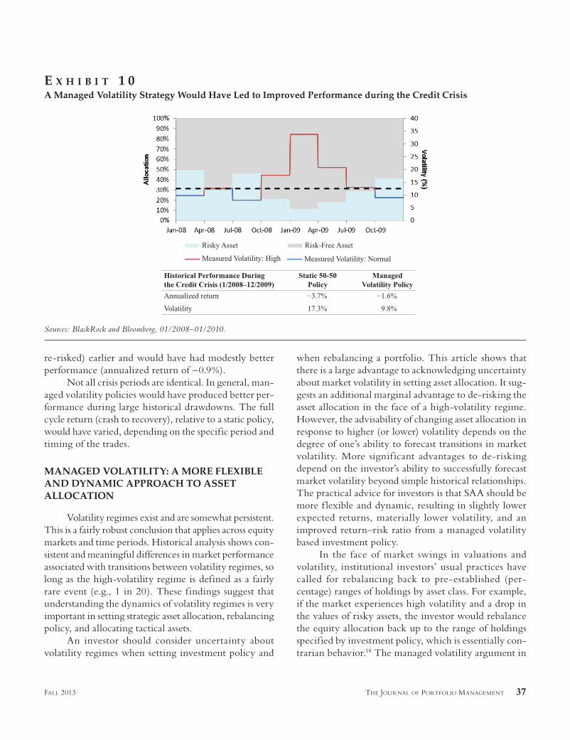
We ask a central question: How would a managed volatility investor have performed during the 2008–2009 credit crisis? We shall answer this with a back test. Con-sider an investor with a 50/50 risky/risk-free policy, represented by the S&P 500 and three-month T-bills, respectively. The policy portfolio has a normal volatility of 7.5% and expected returns consistent with the inves-tor’s objectives. The investor follows a managed vola-tility approach and accordingly sets an upper threshold of 12.5% that defines a significant regime change and calls for a more conservative policy. Specifically, the investor monitors current volatility every quarter, based on the daily returns of the previous quarter, and continues to hold the policy as long as volatility stays below 12.5%. However, in extreme markets when volatility exceeds 12.5%, the investor de-risks the policy back to 7.5% volatility by selling out of a measured amount of risky
assets into the risk-free asset. Subsequently, as portfolio volatility falls, the investor partly reinvests in risky assets to bring volatility back up to the original level, subject to a maximum risky-asset allocation of 50%. In this manner, the investor steps back into the normal policy benchmark, as the benchmark’s underlying volatility falls back below 7.5%. Exhibit 10 illustrates policy allocations during 2008 and 2009, and the table summarizes risk–return characteristics over this period. Volatility fig-ures represent the quarterly volatility of the previous quarter and are used as a signal for policy changes.
The credit crisis was a period of f luctu-ating volatility, resulting in significant changes to the managed volatility policy. Volatility increased over the 12.5% threshold in the f irst quarter of 2008 and then fell back the following quarter, resulting in de-risking and subsequent re-risking. Quarterly volatility
then rose materially in the second half of the year, fol-lowing the Lehman bankruptcy, and peaked at 34% at the end of 2008. This volatility spike would have caused the investor to de-risk the policy to 90% risk-free assets in the first quarter of 2009. In 2009, as the economy stabilized, volatility progressively fell. The policy would have begun to step back into risk assets and would have had 41% in risk assets at the end of 2009. The portfolio would have been back to the original policy allocations in the second quarter of 2010.
Portfolio de-risking would have resulted in smaller drawdowns in 2008, but the managed volatility policy would also have missed out on some of the equity market rally in 2009. Overall, however, the managed volatility policy would have smaller negative returns (−1.6% annu-alized, compared with −3.7% for the static policy) and much more consistency (volatility of 9.8%, compared with 17.3% for the static policy).
This example is meant to be illustrative, and past performance is no indication of future performance. The characteristics and performance of managed volatility strategies will depend on the risk model used, the fore-casting horizon, and the specific period. For example, if we assumed monthly monitoring (as opposed to quar-terly) based on the volatility of the previous month, the managed volatility strategy would have de-risked (and
E X H I B I T 9Dynamic Allocations Have Significant Utility Benefits That Increase with the Ability to Forecast Transitions
re-risked) earlier and would have had modestly better performance (annualized return of −0.9%).
Not all crisis periods are identical. In general, man-aged volatility policies would have produced better per-formance during large historical drawdowns. The full cycle return (crash to recovery), relative to a static policy, would have varied, depending on the specific period and timing of the trades.
MANAGED VOLATILITY: A MORE FLEXIBLE AND DYNAMIC APPROACH TO ASSET ALLOCATION
Volatility regimes exist and are somewhat persistent. This is a fairly robust conclusion that applies across equity markets and time periods. Historical analysis shows con-sistent and meaningful differences in market performance associated with transitions between volatility regimes, so long as the high-volatility regime is defined as a fairly rare event (e.g., 1 in 20). These findings suggest that understanding the dynamics of volatility regimes is very important in setting strategic asset allocation, rebalancing policy, and allocating tactical assets.
An investor should consider uncertainty about volatility regimes when setting investment policy and
when rebalancing a portfolio. This article shows that there is a large advantage to acknowledging uncertainty about market volatility in setting asset allocation. It sug-gests an additional marginal advantage to de-risking the asset allocation in the face of a high-volatility regime. However, the advisability of changing asset allocation in response to higher (or lower) volatility depends on the degree of one’s ability to forecast transitions in market volatility. More signif icant advantages to de-risking depend on the investor’s ability to successfully forecast market volatility beyond simple historical relationships. The practical advice for investors is that SAA should be more f lexible and dynamic, resulting in slightly lower expected returns, materially lower volatility, and an improved return–risk ratio from a managed volatility based investment policy.
In the face of market swings in valuations and volatility, institutional investors’ usual practices have called for rebalancing back to pre-established (per-centage) ranges of holdings by asset class. For example, if the market experiences high volatility and a drop in the values of risky assets, the investor would rebalance the equity allocation back up to the range of holdings specified by investment policy, which is essentially con-trarian behavior.18 The managed volatility argument in
E X H I B I T 1 0A Managed Volatility Strategy Would Have Led to Improved Performance during the Credit Crisis
Sources: BlackRock and Bloomberg, 01/2008–01/2010.
38 MANAGED VOLATILITY STRATEGIES: APPLICATIONS TO INVESTMENT POLICY FALL 2013
this article, applied to this scenario, would not require rebalancing back to the range of original holdings. Instead, holdings would be rebalanced to a (revised) optimal risk–return tradeoff, potentially reducing the extent of contrarian behavior.19 This approach increases the potential f lexibility for institutional investors who are otherwise required to rebalance their portfolio hold-ings at high cost during an investment crisis.
In recent years, institutional investors have de-risked their portfolios by reducing their allocations to the riskiest asset classes, and some did not rebalance back investment policy during the financial crisis. It is unclear whether this behavior was motivated by managed vola-tility principles, tactical investing, or other reasons. Nonetheless, managed volatility is a concrete approach to asset allocation that builds on the historical evidence that volatility is somewhat predictable, and on the principle that an investor may be willing to forgo some expected return for less volatility. When faced with high-volatility regimes, an investor de-risking the portfolio back to an original portfolio risk budget (managed volatility) may be more advantageous than rebalancing back to original holdings of risky assets (traditional practices).
ENDNOTES
The authors gratefully acknowledge valuable insights and contributions from Ben Golub, Phil Hodges, Stuart Jarvis, Ronald Kahn, Russ Koesterich, Ken Kroner, Michael Pensky, John Pirone, Marcia Roitberg, and other colleagues.
1The authors credit this phrase to Professor Robert Engle during a meeting with him and The Volatility Institute of New York University, Stern School of Business.
2Dopfel [2010] proposed a policy portfolio that is revised to account for additional uncertainty associated with dynamic market regimes. Chan and Ramkumar [2010] showed advan-tages to risk-based rebalancing in stressed markets, compared with the usual holdings-based rebalancing.
3Most institutional investors have been trained to stay the course. This seems prudent, based on past experience and on academic studies that have pointed out disappointing results for market timing where the goal was to gain higher realized returns. See Graham and Harvey [1996].
4An investor’s optimal risk–return tradeoff is expressed by deciding what portion of total assets to invest in risky assets (h), with the remainder in a risk-free asset. For an asset-only investor, the risk-free asset is cash and the risky asset is a portfolio composed of equities, (non-Treasury) bonds, real estate, and other asset classes. For a liability-relative investor,
the risk-free asset is the liability-hedging portfolio and the risky asset is a growth portfolio. Assuming a Sharpe ratio of risky assets (SR), excess return (r) and risk (σ) of the risky asset, and risk aversion (λ), the investor seeks to maximize expected utility: ( ( / )2 2( 2EU h2r ( SR hp p( )= r / )λ//2)) σ2
p ⋅ ⋅SR σ − ⋅//2)/2) σ . Optimization conditions result in h = SR/λσ.
5As noted, optimal holdings are h = SR/λσ. The inves-tor’s holdings would remain constant if the expected Sharpe ratio and risk rose in the same proportion and the risk-aver-sion parameter were constant.
6The investor’s portfolio choice in a single-period con-text may be different than in a multi-period setting, depending on the form assumed for the investor’s utility function, the asset return distribution, and the investment horizon. Most often, economists assume that the utility function has linear absolute risk tolerance in wealth. This class of utility functions enables closed-form solutions to the multi-period portfolio problem and ensures the equivalence of single-period and multi-period portfolio choice in the case of serial indepen-dence of asset returns. See Mossin [1968].
7Glosten, Jagannathan, and Runkle [1993] reviewed sev-eral studies that find both positive and negative links between intertemporal risk and return, and they find that the results can be sensitive to the specific volatility measure used.
8We annualize volatility assuming 250 trading days and no serial correlation.
9The results of any regime analysis are necessarily inf lu-enced by the specific period considered. For example, in 2007, an investor who analyzed the previous 50 years would have likely defined a less-extreme measure of high volatility and would have had differing conclusions about the characteristics of each regime. In practice, a longer perspective is recom-mended, but one must use judgment to determine thresholds and whether they change through time.
10All data are annualized based on months classif ied as high volatility and normal volatility, respectively. Mean excess return represents the annualized (arithmetic) average excess return over three-month T-bills.
11For several indices, only daily price return is avail-able for some period after the index’s inception. We approxi-mate daily total returns over these periods by assuming that monthly dividend returns are accrued uniformly throughout the month.
12The MSCI Japan Index stood out as anomalous and actually had a small, positive mean excess return during periods of transition to high volatility. Over the period 1928 to 2011, the S&P 500 would have had ex ante Sharpe ratios of 0.17 and 0.43 in high- and normal-volatility regimes, respec-tively. The lower Sharpe ratio of the high-volatility regime was primarily driven by its greater persistence (65% as com-pared with 36% after 1950) and the higher-volatility periods’ greater volatility over the full sample.
13Monthly forecasting periods resulted in higher persis-tence of high-volatility periods in all cases, except a modest decrease for the Russell 2000 and MSCI EM indices. The ex ante Sharpe ratios of annualized (monthly) high-vola-tility periods were significantly and consistently lower than normal volatility for all indices, with the exception of the Japan index.
14See Bollerslev, Chou, and Kroner [1992] for a survey of volatility-forecasting methods that result in improved accu-racy by incorporating features such as clustering, mean rever-sion, and correlation to negative returns that have empirically characterized volatility.
15These investor types follow Dopfel [2010] with respect to the definitions of “Naive” and “Prophetic” investors. The “Strategic” and “Managed Volatility” investors have replaced the “Smart, But Humble” investor.
16Dopfel [2010] provided an overview of the regime framework for asset allocation and how investors can create portfolios that are hedged against transitions. The investor’s objective is to maximize expected utility: ( ) ( / ) ,2EU r) −r λ σ//2) where λ (equal to 6.5 in this example) is a risk-aversion parameter and r and σ2 are the expected return and variance, respectively, of random portfolio returns r� . The optimal holdings of the risky asset are determined: h = SR/λσ, where SR is the expected Sharpe ratio and holdings are subject to a no-leverage constraint 0 ≤ h ≤ 1. Naive makes a choice of
/, 1,1 1,1 1/ ,1h h SRu, =h λσ independent of, and without knowl-edge of, current state u (believing he is in state 1, low vola-tility), and without foresight on the transition to state v (he believes he will remain in state 1). Strategic makes a choice of h
u,v = h = SR/λσ independent of, and without knowledge
of, current state u, and without foresight on transition to state v, but with full knowledge of the regime framework. Managed Volatility makes a choice of /, ,h h SRu v, u uS u u,=h λσwith knowledge of current state u but without full foresight on transition to state v (only the knowledge of the state-contingent transition probabilities). Prophetic makes choice of , , ,hu v, u v, u v,= λ/SRSS u v σ with full knowledge and with foresight of current state u and transition to state v.
17The high volatility regime is defined as a sufficiently rare event such that the probability of regime transition is low. For example, there is only a 6% probability of normal-high transition. Further, bid–ask spreads for trading most public equity and fixed-income benchmarks are quite modest. As a result, the transaction costs of following a managed volatility approach, particularly with liquid asset classes, should be low and are ignored for simplicity in our analysis. In periods of low liquidity where spreads may widen, investors, particularly those with higher allocations to private assets, can benefit from using derivatives for de-risking. Even in stressed periods, derivatives tend to remain substantially more liquid than the
underlying asset classes and offer a great deal of f lexibility in rebalancing applications. Chan and Ramkumar [2011], for example, describe how investors can use a combination of just S&P 500 and Treasury futures to effectively reduce portfolio risk.
18Sharpe [2010] pointed out that a policy of rebalancing back to original asset holdings is contrarian, because it would buy assets that have done poorly and sell assets that have done well. Further, this policy is not macro-consistent, as it can only be followed by a minority of investors.
19An equilibrium-rebalancing model is beyond the scope of this article.
REFERENCES
Bollerslev, T., R. Chou, and K. Kroner. “ARCH Modeling in Finance: A Review of the Theory and Empirical Evidence.” Journal of Econometrics, 52, 1992.
Chan, L., and S. Ramkumar. “Tracking Error Rebalancing.” The Journal of Portfolio Management, Vol. 37, No. 4 (Summer 2011).
Dopfel, F. “Designing the New Policy Portfolio: A Smart But Humble Approach.” The Journal of Portfolio Management, Vol. 37, No. 1 (Fall 2010).
Glosten, L., R. Jagannathan, and D. Runkle. “On the Rela-tion between the Expected Value and the Volatility of the Nominal Excess Return on Stocks.” The Journal of Finance, Vol. 48, No. 5 (December 1993).
Graham, J., and C. Harvey. “Market Timing Ability and Vol-atility Implied in Investment Newsletters’ Asset Allocation Recommendations.” Journal of Financial Economics, 42, 1996.
Merton, R. “An Intertemporal Capital Asset Pricing Model.” Econometrica, Vol. 41, No. 5 (September 1973).
Mossin, J. “Optimal Multiperiod Portfolio Policies.” The Journal of Business, Vol. 41, No. 2 (April 1968).