Applied Probability Trust (February 11, 2000)RESTARTING SEARCH ALGORITHMS WITH APPLICATIONS TOSIMULATED ANNEALINGF. MENDIVIL, R. SHONKWILER, AND M. C. SPRUILL,� Georgia Institute of Tech-nology AbstractSome consequences of restarting stochastic search algorithms are studied. It isshown under reasonable conditions that restarting when certain patterns occuryields probabilities that the goal state has not been found by the nth epoch whichconverge to zero at least geometrically fast in n. These conditions are shownto hold for (RSA), restarted simulated annealing, employing a local generationmatrix, a cooling schedule Tn � c=n, and restarting after a �xed number r + 1of duplications of energy levels of states when r is su�ciently large. For (SA),simulated annealing, with logarithmic cooling these probabilities cannot decreaseto zero this fast. Numerical comparisons between (RSA) and several modernvariations on (SA) are also presented and in all cases (RSA) performs better.RANDOM SEARCH; STOCHASTIC PROCESS RENEWAL; CODING SCHEDULE;MINIMIZATIONAMS 1991 SUBJECT CLASSIFICATION: PRIMARY 60K20; 60G35; 60J20; 65K10SECONDARY1. IntroductionEvidence that stochastic algorithms can spend excessive time in states other thanthe goal comes most frequently and easily from simulations and more rarely fromtheoretical arguments. For example, an \optimal" cooling schedule (see Hajek (1988))for simulated annealing (SA) guarantees that the probability the search process is inthe goal state tends to 1 as the number of epochs n tends to in�nity; the expected� Postal address: School of Mathematics, Georgia Institute of Technology, Atlanta, GA 30332.1

2 F. MENDIVIL, R. SHONKWILER, M. C. SPRUILLtime taken by (SA) to hit the goal can however be in�nite (see Shonkwiler and VanVleck (1994) or Fox (1995)). Our main results are Theorems 3.1 and 4.1 and theyshow, among other things, that under certain conditions, restarted search processes,particularly simulated annealing with the proper cooling schedule, has �nite expectedhitting time. Restarting (SA) based on di�erent criteria from ours has been studiednumerically as in Atkinson (1992) and Nakakuki and Sadeh (1994). The undesirablyslow convergence of (SA) has also motivated some research like that in Kolonko(1995) and B�elisle (1992) on the random adjustment of the cooling schedule, on non-random adjustments as reported, for example, in van Laarhoven and Aarts (1987) orAndresen and Nourani (1998), and the thorough theoretical treatment of simulatingdirect self-loop sequences in Fox (1995) and the truncated version in Fox and Heine(1995).Most of the literature to date has been devoted to the investigation of the limitingprobability the process is found in the goal states and sometimes (see for exampleChiang and Chow (1988)) to the rate of convergence of these probabilities. FollowingShonkwiler and Van Vleck (1994), we take a somewhat di�erent approach. The bestan algorithm has done up to epoch n is easily recorded and accordingly our resultsare stated in terms of the probabilities of not yet seeing the goal by the nth epochrather than in terms of the probability of being in the goal state at the nth epoch.We call the probabilities of not yet seeing the goal by the nth epoch tail probabilities(not to be confused with measure-theoretic notions of the same name as found forexample in Niermiro (1995)). Theorem 3.1 provides su�cient conditions for generalsearch processes to guarantee geometric convergence of the tail probabilities to zerounder restarting after user speci�ed patterns and Theorem 4.1 specializes these tothe case of restarting simulated annealing. Of course, in both cases expected hittingtimes must be �nite.Fix an arbitrary stochastic algorithm for minimizing a function over the �nite setC, a function f to be minimized, and let G be the goal subset determined by f .Let Xn be the candidate point in C dictated by the algorithm at epoch n for whatvan Laarhoven and Aarts (1987) would term this problem instance. The sequence ofrandom variables Xn is a C-valued stochastic process and its law of motion, which of

Restarting Search Algorithms 3course should depend upon f , can be quite general. The process Xn is not assumedto be Markov, just adapted to a �ltration fFn : n � 1g. One could study alternativerestarting rules but the one analyzed here involves repeated instances of energy levelsf(Xn) of states and hence hitting times of the vector process of r+1 states with valuesin Cr+1 = C�C�� � ��C called the r-process. Upon the event of the r-process lyingin a certain �xed subset of Cr+1 the algorithm is restarted at a randomly selectedpoint, always using the same distribution as the one used in the initial choice.The analysis of this scheme is shown to be amenable to techniques from discrete timerenewal theory. Hu et al. (1997) had previously utilized renewal equations to analyzerestarting from speci�c subsets of the domain C. There, they showed that under someconditions, the tail probabilities decrease geometrically to 0. Their results extendedand related earlier results, based on the Perron-Frobenius theory, which Shonkwilerand Van Vleck (1994) obtained for Markov algorithms. The restarting process studiedby Hu et al. is implementable in practice only when there is special knowledge of thefunction to be minimized and the algorithm. Restarting from an arbitrary state canbe detrimental to the progress of the algorithm towards the goal and one may notknow, a priori, which states are the correct ones to initiate restarting. Restarting onrepeated energy values alleviates this problem.Fox's work on self looping in (SA) and especially the truncated version in Fox andHeine (1995) is closely related to the method of restarting (SA) on the diagonal, butthere are some key di�erences. Foremost perhaps is that Fox's calculation of theobjective function at each neighbor of the points visited is not required.Andresen and Nourani (1998) propose a constant thermodynamic speed coolingschedule for (SA) and compare its performance for solving a permanent problem witha variety of other cooling schedules. We present a comparison of our method withthese several methods on a permanent problem also.The paper is organized by section as follows. In section 2 the restarted processand the r-process are de�ned and the tail probabilities are shown to satisfy a renewalequation. In section 3 rate of convergence to zero of the tail probabilities is studied.Section 4 deals with simulated annealing where su�cient conditions for geometricconvergence of the tail probabilities are presented. The outcomes of simulations

4 F. MENDIVIL, R. SHONKWILER, M. C. SPRUILLcomparing (SA) with (RSA) are presented in section 5 along with some comments onthe selection of the parameter r.2. The restart and r-processesRestarting when a sequence of states lies in a subset D of Cr+1 de�nes a newprocess on the original search process. Details of this de�nition and the fact that thetail probabilities for the r-process satisfy a renewal equation are presented here.We assume that the goal set G is a non-empty subset of the �nite set C. Fix r � 1,let D be a subset of Cr+1 and de�ne for subsets A of C the setsDA = f(x1; x2; : : : ; xr+1) 2 D : x1 2 Ag :Denote by E the set E(t) = �x 2 CnG : P �(Xn; Xn+1; : : : ; Xn+r) 2 D j Xn = x andall histories up to n� � t for all n 6= ; for some �xed t > 0, and let U = G[E. Hereand below, by informal expressions like P [(Xn; Xn+1; : : : ; Xn+r) 2 D j Xn = x andall histories up to n] � t, we mean the more pedanticP [(Xn; Xn+1; : : : ; Xn+r) 2 D j Fn] � ton the event Xn = x. Introduce the following two conditions, where TE = minfn :Xn 2 Eg.(A1) 1 > P [TE < TG] > 0.(A2) There is a �nite K � 1 and a number � 2 (0; 1) such that uniformly forx 2 CnG, and all n,P [TU > m+ n j Xn = x and all histories up to x] � K�m;where the probability on the left hand side is that the �rst epoch after n atwhich the X process lies in U is greater than m+ n.Let fX(j)n : n � 1g be iid copies of the process X and de�neN(j) = minnn : (X(j)n ; X(j)n+1; : : : ; X(j)n+r) 2 D or X(j)n 2 Goor N(j) = +1 if the set above is empty.

Restarting Search Algorithms 5Lemma 2.1 Under (A2), P [N(j) <1] = 1.Proof. We haveP [N(1) > m j X(1)1 = x]=XP [X(1)m+r = x(m+ r); : : : ; X(1)3 = x(3); X(1)2 = x(2) j X(1)1 = x];where the sum extends over x(2); : : : ; x(m+ r) with no segment of length r+1 in D.With U as above de�neK(x(1); x(2); : : : ; x(m)) = minfj � 1 : x(j) 2 Ugor +1. ThenP [N(1) > m j X(1)1 = x] = mXj=1 pj(x)P [N(1) > m j K = j] + qm(x)Certainly, since there are more paths from x at 1 to x(m) at m which do not touchU than there are which don't touch U and don't have segments in Dqm(x) � P [TU > m j X(1)1 = x] � K�m�1and since given U �rst hit at j � m, N(1) > m entails,P [N(1) > m j K = j] � 1� t:Therefore, P [N(1) > m j X(1)1 = x] � K�m�1 + 1� t:ChooseM so large thatM > r+1 and K�M�1+1� t = � < 1. If Aj is the event of arun of length at least r+1 of states in C for epochs n 2 [(M + r)j+1; (M + r)j+M ]then conditioning shows that P 24 j+k\i=j+1Aci35 � �k;so that P [Aj i. o.] = 1.

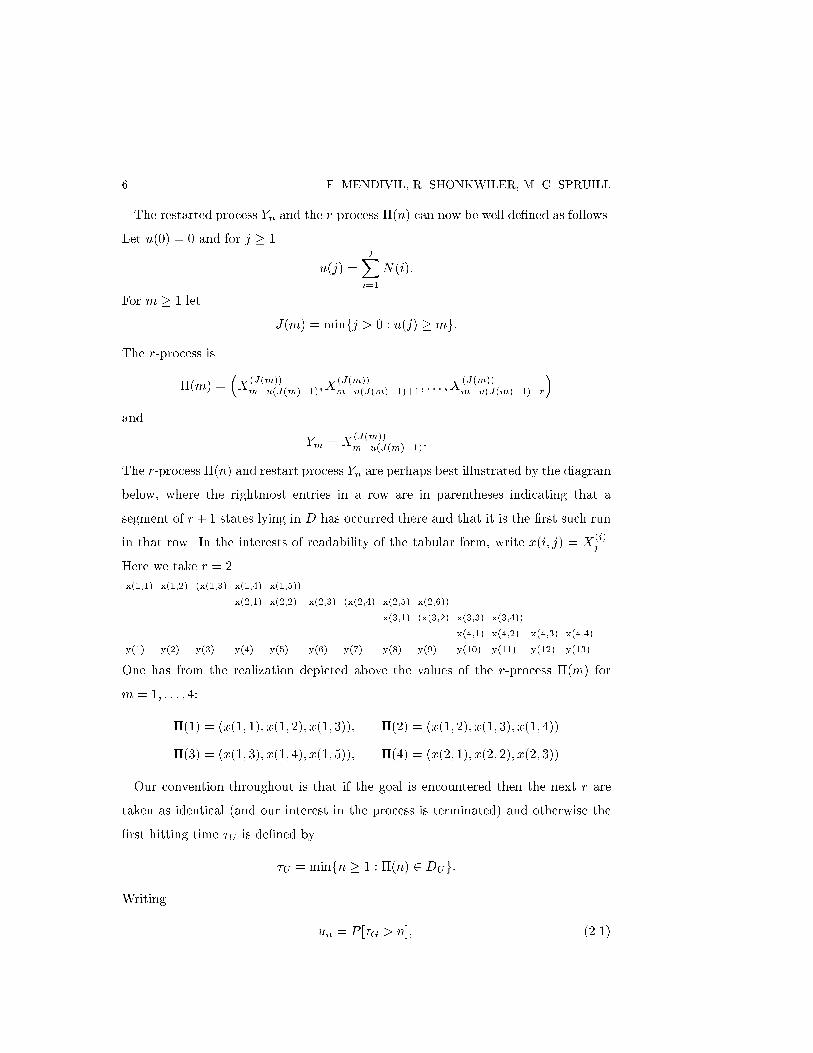
6 F. MENDIVIL, R. SHONKWILER, M. C. SPRUILLThe restarted process Yn and the r-process �(n) can now be well de�ned as follows.Let u(0) = 0 and for j � 1 u(j) = jXi=1 N(i):For m � 1 let J(m) = minfj > 0 : u(j) � mg:The r-process is�(m) = �X(J(m))m�u(J(m)�1); X(J(m))m�u(J(m)�1)+1; : : : ; X(J(m))m�u(J(m)�1)+r�and Ym = X(J(m))m�u(J(m)�1):The r-process �(n) and restart process Yn are perhaps best illustrated by the diagrambelow, where the rightmost entries in a row are in parentheses indicating that asegment of r+1 states lying in D has occurred there and that it is the �rst such runin that row. In the interests of readability of the tabular form, write x(i; j) = X(i)j .Here we take r = 2.x(1,1) x(1,2) (x(1,3) x(1,4) x(1,5))x(2,1) x(2,2) x(2,3) (x(2,4) x(2,5) x(2,6))x(3,1) (x(3,2) x(3,3) x(3,4))x(4,1) x(4,2) x(4,3) x(4.4)y(1) y(2) y(3) y(4) y(5) y(6) y(7) y(8) y(9) y(10) y(11) y(12) y(13)One has from the realization depicted above the values of the r-process �(m) form = 1; : : : ; 4:�(1) = (x(1; 1); x(1; 2); x(1; 3)); �(2) = (x(1; 2); x(1; 3); x(1; 4))�(3) = (x(1; 3); x(1; 4); x(1; 5)); �(4) = (x(2; 1); x(2; 2); x(2; 3))Our convention throughout is that if the goal is encountered then the next r aretaken as identical (and our interest in the process is terminated) and otherwise the�rst hitting time �U is de�ned by�U = minfn � 1 : �(n) 2 DUg:Writing un = P [�G > n]; (2.1)

Restarting Search Algorithms 7one has upon decomposition of the event f�G > ng asf�G > ng = f�U > ng [ (f�G > ng \ f�U = 1g)[ � � � [ (f�G > ng \ f�U = ng)that un = bn + nXj=1 P [f�G > ng \ f�U = jg] = bn + nXj=1 un�jfj ;where fn = P [�G > n, �U = n] and bn = P [�U > n]. Therefore, the tail probabilitiesun for the r-process hitting times satisfy a renewal equation.3. Finite expected hitting time and geometric decrease of tail probabilitiesRapid convergence of the tail probabilities un = P [�G > n] is established in thissection. It follows from (A1) thatXj�1 P [�G > j; �U = j] < 1;for Pj�1 P [�G > j; �U = j] = P [�E < �G] and the latter probability can be seen tobe in (0; 1) as follows. The di�erences in the times at which � hits D are clearly iidand each such time di�erence is the result of one of precisely three types of events;either the X process has a succession of r + 1 states for which the � process is inDUc , or a succession of r + 1 states for which � is in DE, or one of the states in Gis hit (once) at that epoch. Let q, pE , and pG denote the respective probabilities ofthese three types of hits, with q = 1� pE � pG. These are numbers de�ned by the Xprocess. The conditional probability the stop was of type E given that the stop wasof type U is P [�E < �G] = pEpE + pGwhich under the condition (A1) is clearly not zero or one.Theorem 3.1 Under the conditions (A1) and (A2), E[�U ] < 1, E[�G] =E[�U ]1�P [�E<�G] <1, and there is a 2 (0; 1) and a �nite constant c such that �nun ! cas n!1, with un given by (2.1).

8 F. MENDIVIL, R. SHONKWILER, M. C. SPRUILLProof. To begin, we prove that 1 < lim infk!1 f�1=kk . Since the event (�G >n) \ (�U = n) implies the event (�U > n � 1), one has fn � bn�1 for all n andlim infk!1 f�1=kk � lim infk!1 b�1=kk . We will show below that lim infk!1 b�1=kk >1. Assuming this for the moment, it would follow that both of the power seriesb(z) = Pn�0 bnzn and f (z) = Pn�1 fnzn have radius of convergence greaterthan 1. On a su�ciently small neighborhood of 0 one hasu(z) = b(z) + f (z)u(z) (3.1)where u(z) =Pn�0 unzn and un is given by (2.1). Since the power series f (z) hasradius of convergence greater than 1 andPn�1 fn < 1, the function b(z)=(1�f(z))is holomorphic in an open set containing the unit disc. Therefore, u(z) has radiusof convergence greater than 1 and it follows that there is a 2 (0; 1) and a �niteconstant c such that �nun ! c as n!1. Furthermore, (see also Feller (1968))E[�G] =Xn�0un = b(1� f) :To complete the proof decompose the event (�U > n), using H = minfj : �(j) 2DCnUg, as (�U > n) = n[j=1 ((�U > n) \ (H = j)) [ (H > n) \ (�U > n):Then P [�U > n] = nXj=1 P [(�U > n) \ (H = j)] + P [(H > n) \ (�U > n)]= nXj=1 P [�U > n j (H = j) \ (�U > j)]P [(H = j) \ (�U > j)] + cn= nXj=1 P [�U > n� j]kj + cn:Since Pj�1 kj = P [� hits DCnU before DU ] < 1, if we can show lim infk!1 c�1=kk >1 then we'll have by application to P [�U > n] of the arguments above applied toun, that lim infk!1 b�1=kk > 1. But cn is the probability of no restarts in the �rstn epochs so consulting Lemma 2.1, for n = k(M + r) + d, 0 � d < M + r � 1,cn � �k � K�n, where K = �1=(M+r)�1 > 1 and � = �1=(M+r) < 1.

Restarting Search Algorithms 9The constant c in Theorem 3.1 may be zero and the rate of convergence could befaster than geometric. Sometimes the series b(z) and f (z) satisfy conditions underwhich the rate can be established precisely as follows.Corollary 3.2 If (A1), and (A2) hold, if fn is not periodic and there is a realsolution � > 1 to f (�) = 1 satisfying b(�) < 1 then there is a � 2 (0; 1) and a�nite positive constant c such that ��nun ! c as n!1.Proof. Taking � = 1=�, setting vn = �nun, the vn satisfy a renewal equationvn = Bn + nXj=1 vn�jFj ;with Bn = �nbn and Fn = �nfn. Under aperiodicity of the fn, Theorem XIII.10.1of Feller (1968) yields the conclusion and the precise rate of convergence if b(�) =PnBn <1.By restarting, the expected time to goal of a search process can be transformedfrom in�nite to �nite. Multistart, (see Schoen (1991)) where under no restartingthe hitting time is in�nite with positive probability, is an obvious example. Undersimple conditions like restarting according to a distribution which places positivemass on each state, multistart trivially satis�es the conditions (A1) and (A2) witht = 1. Furthermore the conditions of Corollary 3.2 hold and it provides an interestingformula for the Perron-Frobenius eigenvalue as the reciprocal of the root of a lowdegree polynomial (see Hu et al. (1997)). More subtle is the (SA) Example 4.3 below.Of course it is easy to construct, as in the next example, a search process whichmakes a restarting scheme perform, unless it is done correctly, worse than the originalalgorithm.Example 3.3 Let the state space be f0; 1; 2g with 0 as the goal. Suppose for alln � 2 P [Xn+1 = i j Xn = j;Xn�1 = k] = 8>>>><>>>>:1 if i = 0 and j = k = 11 if i = 1 and j = 1 and k 6= 11 if i = 1 and j 6= 1

10 F. MENDIVIL, R. SHONKWILER, M. C. SPRUILLand P [X2 = i j X1 = j] = 1 if i = 1 and 0 otherwise. Restarting whenever arepeated state occurs is clearly detrimental in this case since the original process goesdeterministically directly to the goal as quickly as possible, but must repeat the state1 before doing so. Restarting after 3 the same however does not hinder the original.4. Application to simulated annealingThe generality of the conditions in Theorem 3.1 suggests the possibility of discover-ing particular algorithms or classes of algorithms exhibiting these general underlyingfeatures and hence also ones for which restarting results in the rapid decrease of thetail probabilities. One instance of this is simulated annealing. Let the generationmatrix Q be �xed (see any standard reference on (SA) such as van Laarhoven andAarts for terminology) and introduce the following assumption (A3) which we willinvoke at the appropriate time. Let fN(x) : x 2 Cg be a collection of subsets of C,one for each distinct x, which we call neighborhoods of x, having the property thatfor any x; y in C there is a �nite sequence z(1); z(2); : : : ; z(j) of points in C such that,setting x = z(0) and y = z(j+1), z(i+1) 2 N(z(i)) for all i = 0; 1; : : : ; j. We assumealso that y 2 N(x) entails x 2 N(y).(A3) - The generation matrix Q allows only transitions to the immediate neighbors sothat qxy = 0 unless y 2 N(x), assigns positive mass to each of them so that qxy 6= 0for y 2 N(x)nfxg and qxx = 0.Consider the minimization of a function f de�ned on the �nite set C. Leta = minx2C miny2N(x)ff(y)� f(x) : f(y)� f(x) > 0g;where N(x) is the collection of immediate neighbors in C of x. Since C is �nite,� > 0. Let the acceptance rule be the usual with(A4) the probability of accepting a transition from x to y 6= x at epoch n being givenby minf1; e�(f(y)�f(x))=c(n)g, where c(n) is strictly decreasing to 0 with increasing nand the probability of a transition from x to x is one minus the sum of the probabilitiesof transitions from x to all other states.The binary relation x�y if f(x) = f(y) de�ned on C�C is an equivalence relation so

Restarting Search Algorithms 11that C can be partitioned into disjoint equivalence classes C1; : : : ; Ck. Furthermore,the relation x � y de�ned on Cj by x � y if x and y are in Cj and there is a pathfrom x to y, x = z0, zi 2 N(zi�1), i = 1; : : : ; k, zk = y, some k < 1, and zi 2 Cjfor every i is an equivalence relation. The set C is thereby partitioned into disjointsubsets Bij . Such a subset B is a basin bottom if for every x 2 B and y 62 B everypath z0; : : : ; zk from x to y has f(zj) > f(zj�1) for some j.In the following theorem the subset D is the set of points in Cr+1 such that f(x1) =� � � = f(xr+1).Theorem 4.1 Under conditions (A3){(A4) above and if there is � > 1 such thatXn�1�ne��=c(n) <1 (4.1)then under restarting (SA) by a distribution which places positive probability on eachpoint in C for r, 1 � r < 1, su�ciently large there is a 2 (0; 1), and a �niteconstant c such that �nun ! c as n!1.Proof. The method of proof is simply to employ the structure of this particularalgorithm and the assumptions made in the hypotheses to check that the appropriateconditions of Theorem 3.1 are met.We turn �rst to the set E. Let W (a candidate for E which we will show worksfor an appropriate r) denote the union of the disjoint basin bottoms associated withnon-global minima. Let V = G [W .For any x 2 B, a basin bottomP [f(Xn+1) = f(Xn) j Xn = x] = 1� Xf(z)>f(x) qxze�(f(z)�f(x))=c(n)� 1� Xf(z)>f(x) qxze��=c(n)= Xf(z)=f(x) qxz + Xf(z)>f(x) qxz(1� e��=c(n))� Xz2N(x) qxz(1� e��=c(n)) = 1� e��=c(n):

12 F. MENDIVIL, R. SHONKWILER, M. C. SPRUILLFurthermore, if x 2 B, y 2 N(x), and f(y) = f(x), then y 2 B also so, letting forx 2W , a(r; x) = P [f(X1+r) = � � � = f(X1) j X1 = x], it is clear thatln(P [f(Xn+r) = � � � = f(Xn) j Xn = x]) � ln(a(r; x))� r+1Xj=1 ln(1� e��=c(j)) � r+1Xj=1 e��=c(j)1� e��=c(j)� � 11� e��=c(1) e��=k 1� e��(r+1)=k1� e��=k :Therefore, for each x 2 W there is a c(x) > 0 such that a(r; x) � c(x) for all r. Now� = minx2W c(x) must be positive since it is the minimum over a (non-empty ) �niteset of positive numbers. For any t 2 (0; �) one will have for all nP [(Xn; Xn+1; : : : ; Xn+r) 2 D j Xn = x and all histories up to n] � tfor all x 2 W . We will see below that for all x in CnG which are not in W this failsfor some n and therefore we can take W = E(t).The transition matrices Pn converge to the matrix P and the xy element of Pn�Pis (Pn � P )xy = qxye�(f(y)�f(x))=c(n)if f(y) > f(x) and 0 otherwise. The limiting matrix P has xy element qxy if y 2 N(x)and f(y) � f(x) and 0 otherwise. The submatrix S of P which corresponds to thestates in Gc\W c has spectral radius less than 1 since every state communicates withat least one state, say x, therein for which f(y) < f(x) for some y 2 N(x) and y is ina basin bottom. Therefore, in the limiting chain, with positive probability at least qxyone leaves the setGc\W c never to return. With Sn the submatrix of Pn correspondingto the states in Gc \W c one has for the matrix norm kAk = maxiPj jaij jkSn � Sk � maxx Xy2N(x) qxye�(f(y)�f(x))=c(n) � e��=c(n)so by the assumption of Theorem 4.1, Pn�1 �nkSn � Sk < 1, for some � > 1. ByLemma (A1) it follows that for some 2 (0; 1) and all m and n,kSmSm+1 � � �Sn+m�1k � E n:

Restarting Search Algorithms 13Since for x 2 Gc \W ce0xSmSm+1 � � �Sn+m�11 = P [(Xn+m�1 2 Gc\W c)\� � �\(Xm 2 Gc\W c) j Xm�1 = x]with U = G [W one has for x 2 Gc \W cP [TU > m+ n j Xm = x and all histories up to x] � K n:If x 2 W then a transition will either occur immediately to W or to W c so (A2)holds.Furthermore, as promised above, W satis�es the requirements of E, for if x 2Gc \W c thenP [(Xn; Xn+1; : : : ; Xn+r) 2 D j Xn = x] � e0xSnSn+1 � � �Sn+r�11 � K rsince a transition to G[W would entail a decrement in the value of f(X). Therefore,for r su�ciently large all elements x 2 Gc \W c will fail the test of being in W .Therefore, for the r we chose above, restarting results in a �nite expected �rsthitting time and convergence to 0 of P [�G > n] at least geometrically quickly.Corollary 4.2 The (RSA) algorithm which uses the local generation scheme sat-isfying (A3), the standard acceptance scheme of (A4), and a cooling schedule ofc(n) = 1=n will, for su�ciently large r, under (A5) have tail probabilities whichconverge to 0 at least geometrically fast in n.The conditions of Theorem 4.1 are not necessary for the geometric convergence ofthe tail probabilities. In the following example, geometric rate of decrease of thetail probabilities is shown for a restarted simulated annealing which uses the usuallogarithmic cooling schedule and a generation matrix which does not satisfy (A3).This example is one for which the (SA) satis�es the conditions of Hajek's theorembut which, without restarting, has an in�nite expected hitting time of the goal.Example 4.3 The Sandia Mountain example provided by Shonkwiler and Van Vleck(1994) as an illustration that independent identical parallel processing can make theexpected time to hit the goal go from in�nite to �nite is presented here from the

14 F. MENDIVIL, R. SHONKWILER, M. C. SPRUILLperspective of restarting when a state is repeated; we show, by showing that theconditions of Theorem 3.1 are met, that the expected time to goal can be made �nitesimply by restarting on the diagonal. The Sandia Mountain function, for N = 4,is piecewise linear from (0;�1) to (1; 1) and from there to (0; 4). In their examplesimulated annealing is applied to the search for the global minimum of the functionf(x) de�ned on f0; 1; 2g by f(0) = �1, f(1) = 1, f(2) = 0, Sandia 2. They showedthat the expected hitting time for the simulated annealing process whose generationmatrix is Q = 266640:5 0:5 0:00:5 0:0 0:50:0 0:5 0:537775and which results, under the cooling schedule T , in the Markov transition matricesP = 266641� 12e�2=T 12e�2=T 01=2 0 1=20 12e�1=T 1� 12e�1=T37775is in�nite when the traditional cooling schedule T = Cln(n+1) , C = 1, n being theepoch number, is used. The generation matrix here does not satisfy assumption (A3)but we show that nevertheless the tail probabilities do converge to zero geometricallyquickly even using the logarithmic schedule. First, under equally likely restarting(A1) is clearly satis�ed. For (A2), note that U = f0; 2g, G = f0g, E = f2g, so thatP [TU > m+ n j Xn = 1] = 0 for any m � 1 and n � 1. If Xn = 2 then either thereis an immediate transition back to U or one to Uc followed immediately by one to Uso that for m = 1 P [TU > m+ n j Xn = 2] = 12e�1=Tand otherwise is this is 0 so (A2) is satis�ed with any � 2 (0; 1). For N = 2 ofExample 4.3 the non-restart case was terminated if it took longer than 40 epochs.Median search times were 3 for restarting and 40 for not.Obviously, geometric or faster decrease to 0 of the tail probabilities P [�G > n] under(RSA) or otherwise entails a �nite expected hitting time of the goal states G, butby itself geometric decrease of the tail probabilities is not a strong recommendation.

Restarting Search Algorithms 15Although a direct comparison of expected times to goal for the two processes (RSA)and (SA) seems unattainable, Example 4.3 shows that this geometric convergence ofthe tail probabilities is not a feature of (SA). We make some informal observationsunder the assumption that both processes use the same generation matrix with (SA)using a logarithmic schedule Tn = c= ln(n + 1), c � d�, and (RSA) using a linearschedule Tn = 1=n. Assume a common position of the two algorithms at epoch n.Since the r-process is de�ned on a di�erent space the two processes will be taken tohave a common position at epoch n if the most recent coordinate of the r-process atepoch n coincides with that of the (SA) process. At any instant of time at which thetwo processes happen to reside at the same \location" the cooling schedule of one,which is logarithmic, should be compared with that of the other, which is linear inthe (random) age of the process, for this will indicate the relative tendencies of goingdownhill. If r is small then the clock will likely have been reset for (RSA), but ifr is large then very likely the r-process will not have restarted at all and the epochnumber will also be the current age. It is the latter instance which is of interest since(RSA) is assumed to have r \large." At a location which is not a local minimumthe (SA) process will have, as the epochs tick away, an ever increasing tendency incomparison with (RSA) to proceed in uphill directions. Thus (RSA) should proceedmore rapidly downhill than (SA) at points which are not local minima.What happens when (SA) and (RSA) are at a local minimum at the same epoch?Very likely the (RSA) will be out of this \cup" (see Hajek) in r steps whereas the(SA) will take some time. Since the goal cannot be reached until the process gets outof the cup this is a crucial quantity in determining the relative performance of thetwo methods when there are prominent or numerous local minima. The (RSA) willhave an immediate chance of �nding the cup containing the goal whereas, dependingupon the proximity of the present cup to the one containing the goal, (SA) may beforced to negotiate many more cups.It follows from Fox and Heine (1995) and Fox (1995) that the enriched neighborhoodversion of QUICKER-j has tail probabilities converging geometrically quickly to 0.An interesting question to which we have no answer is how these two compare. Inour obviously completely unbiased opinion, (RSA) should perform better; only small

16 F. MENDIVIL, R. SHONKWILER, M. C. SPRUILLprescribed numbers of function values in small neighborhoods need be computed andprogress downhill is faster.5. Numerical comparisonsSome numerical results are presented comparing the performance of various formsof (SA) to (RSA). The comparisons were carried out for three types of problems,minimization of a univariate function, minimization of tour length for some TSP's,and �nding the maximum value of the permanent of a matrix. In each case aparameter enters which has considerable in uence on the performance of the method;for standard (SA) it is the constant C in the cooling schedule Cln(n+1) and for (RSA)it is the number r + 1 of energies duplicated before restarting. We attempted tochoose good values of the parameters. When the univariate function or the TSP hada known optimal tour length, the constant C for (SA) was set appropriately accordingto the results of Hajek. More precisely in the terminology of Fox (1995), we chosehis \fTkg" schedule. For the other cases of (SA) an attempt was made to estimatethe correct depth to use Fox's schedule. For setting the parameter r of (RSA) weemployed an heuristic argument based upon the following.In (RSA) it seems desirable to proceed as quickly as possible to points where thefunction has a local minimum and then, if necessary, to restart. Rushing to restartis undesirable however for local information about the function is indispensable incharting a course to a local minimum; by prematurely restarting, this information islost. Therefore one should take care to stay su�ciently long in a location to examinea large enough collection of \directions" from the current point to ensure that pathsto lower values are discovered. For functions on the line there are only two directionsso one would expect to require very few duplications before the decision to restartis made. Were the selection of new directions deterministic, clearly at most twowould be required, but the algorithm chooses these stochastically. In contrast, fora TSP on a reasonable number of cities, if the neighborhood system arises from a2-change (see Aarts and Korst (1989)) then one should presumably wait for a fairlylarge number of duplications to make sure enough \directions" have been examined.

Restarting Search Algorithms 17As a rough guide we note that in (SA) as long as the state has not changed, thegeneration matrix yields a sequence of iid \directions." Assuming the proportion ofdirections downhill is p and uniform probability spread over those directions by thegeneration matrix, the probability the generation matrix has not yielded a downhillafter m generations is simply (1 � p)m. To make this quantity small, say less than�, m should be approximately ln(�)= ln(1 � p). On the line the most interestingplaces are where one direction is up and the other down so p � 1=2 seems reasonable.Furthermore, the consequences of restarting are minimal so a large �, say 1/2, alsoseems reasonable. Thus one should take r around 1. In a TSP with 100 citiesrestarting can be costly since the considerable time it takes to get downhill will likelybe wasted upon restarting. Thus we take � small, say :01. It is not clear what p shouldbe. Presumably the \surface" represented by the tour lengths could be rather roughso we'll take p = :05 to ensure a thorough although perhaps too lengthy examinationof directions. This translates to run lengths of r � 100 and an examination of a fairlysmall proportion of the 4851 \directions" available under 2-change.Example 5.1 For a randomly generated function the median number of epochsrequired to �nd the global minimum by (SA) under optimal cooling, with the stipu-lation that the search was terminated at 221 epochs if the minimum had not yet beenfound, was 221. For (RSA) with r = 1 the median number of epochs required to �ndthe global minimum of the function was 21.Example 5.2 In this example an optimal 100 city tour was sought using 2-change asthe neighborhood system with equally likely probabilities for the generation matrix.The locations were scaled from a TSP instance known as kroA100 taken from a database located on the WEB athttp://softlib.rice.edu/softlib/catalog/tsplib.html.Each of (SA) and (RSA) was run for 1000 epochs. The median best tour lengthfound by (SA) was of 35.89 with a minimum of 34.06. For (RSA) the median besttour length found in 1000 epochs was 14.652 with a minimum of 13.481.Example 5.3 A 24-city TSP instance known as gr24 obtained from the same database as kroA above was analyzed again using 2-change for the neighborhood system

18 F. MENDIVIL, R. SHONKWILER, M. C. SPRUILLand equally likely choices for the generation matrix. Each of (SA) and (RSA) wasrun for 500 epochs. The best tour lengths found by (SA) had a median of 2350.5 anda minimum of 1943. (RSA) with r + 1 = 24 had a median best tour length after 500epochs of 1632.5 with a minimum of 1428. The optimal length is 1272. A similarresult on 24 cities was obtained by running the two for 1000 epochs. Under (SA)the median was 2202 with a minimum of 1852 while for (RSA) the median best tourlength was 1554.5 and minimum 1398.Example 5.4 Performance of (SA) with depth 40 and (RSA) with r = 100 wascompared on a randomly generated 100-city TSP. Median best tour length after 1000epochs for (SA) was 43.14 and the minimum was 40.457. For (RSA) the median bestwas 19.177 and the minimum best was 17.983.Example 5.5 We also tested the performance of our method in comparison withseveral other (SA) cooling schedules employed by Nourani and Andresen (1998) onthe problem of optimizing the permanent of 0-1 matrices. The permanent of an n�nmatrix M is de�ned to be perm(M) =X� nYi=1mi;�(i)where the sum extends over all permutations � of the �rst n integers. The permanentis simply the determinant without the alternating signs. Allowing the matrix elementsto be only 0 or 1, for a given matrix size n and number d of 1's, 0 < d < n2, theproblem is to �nd the matrix having maximum permanent.This problem is simple and scalable being completely determined by the two integervalues, n and d, the matrix size, and its number of 1's. As n grows the problembecomes harder in two ways. First the di�culty in calculating a permanent growsas n! since the number of possible permutations � grows as n!. Second, the numberof possible 0/1 matrices grows as 2n2 . The di�culty also depends on d in that for agiven n, smaller values of d yield fewer non-zero terms in the sum in the calculationof perm(M) while for d � n2 almost all n! terms need to be computed.Nourani and Andresen (1998) studied their constant thermodynamic simulatedannealing cooling schedules with various cooling schedules.

Restarting Search Algorithms 19Figure 1

Figure 1. Simulated annealing for the permanent problem with various cooling schedulesTo compare the several approaches for solving this problem, we �xed n = 14 andd = 40. This gives the number of possible arrangements of the 1's, the size of thesearch space, to be �19640 � or about 8:3 � 1041. These values for n and d result ina permanent calculation that is fast enough that millions of permanent calculationscould be tried in a few minutes; this was necessary for one of the approaches.In all the experiments reported below, our neighborhood system for the simulatedannealing was de�ned by allowing any 1 appearing in the matrix to move one positionup or down or to the left or to the right. In this, we allowed wrapping, that is, a 1on the bottom row could swap positions with a 0 on the top row and similarly forthe �rst and last columns. In this way, each solution, or arrangement of d 1's, hasapproximately 4d neighbors.The \energy" of the annealing, to be minimized, was taken as the negative of thepermanent itself and the cooling schedules we tested were geometric, inverse log,inverse linear, linear, and dynamic as described in Andresen and Gordon (1994),Nulton and Salamon (1988), and Nourani and Andresen (1999). Temperature rangedfrom on the order of 6 down to the order of 0.2. For each di�erent cooling schedule,we tried several temperature ranges until we found one that seemed to work well.Thus, we compared the \best" runs for each cooling schedule.For the restart method, we also ran experiments with these cooling strategies except

20 F. MENDIVIL, R. SHONKWILER, M. C. SPRUILLFigure 2

Figure 2. Restart for the permanent problem with various cooling schedulesfor the dynamic strategy. We took the restart repeat count, r + 1, to be 160.The results are displayed in Figures 1{3 and are the averages of 10 runs. Asseen in the �gures, this problem displays a de�nite \phase transition" in terms ofnormal annealing. This phase transition occurs for temperatures in the neighborhoodof 1. The di�erent schedules reached 1 at di�erent times during their run givingrise to the di�erent times for their precipitous fall. All of the simulated annealingapproaches which spent some time above and below the phase transition temperatureperformed about the same, achieving minima on the order of �1000. As can be seen,all the annealing approaches got stuck and ceased to �nd improvement when theirtemperature dropped below the phase transition temperature.By contrast, the restart algorithm made both very rapid progress at the beginningof the runs and continued to make progress even up to the time the runs were halted.All the annealing runs with restart consistently achieved solutions on the order of�1500. The restarting step was e�ective in allowing the algorithm to escape fromlocal minima even at temperatures below the critical temperature (of approximately1) where the phase transition occurs.We do not know the absolute minimum for this problem, but the best energy seenin any of the runs in all the experiments was �2016.Of special note is the dynamic cooling schedule (see Andresen (1996) for details).

Restarting Search Algorithms 21Figure 3

Figure 3. Restart versus the best standard annealer for the permanent problemIn order to use this approach, one must perform preliminary runs in order to gather\in�nite temperature" energy density and transition statistical data. We found thisto be very hard to do and very costly with essentially no payo� in terms of bene�t.Even after forty eight million iterations at the (practically) \in�nite temperature" of100, there was still no statistical data for energies below �400. Furthermore, we foundthat the statistical technique for estimating the second largest eigenvalue (necessaryto compute the internal relaxation time of the statistical system, see Andresen (1996))entailed so much error as to be practically useless. Instead we directly calculated thiseigenvalue from the estimated transition matrix. For this problem, the e�ort requiredto gather the (incomplete) statistical data in order to start simulated annealing runswith the dynamic cooling schedule is better spent in annealing using some othercooling schedule.An alternative, more careful, analysis of the size of r is provided by closer exami-nation of the proof of Theorem 4.1. Under the cooling schedule c(n) = 1=n with anequally likely generation matrix the choicer � �e��(1� e��)2 1ln(1� p)will guarantee the conclusion of the theorem under its other hypotheses, where p =1 � is the worst case, smallest probability of a downhill from among the points in

22 F. MENDIVIL, R. SHONKWILER, M. C. SPRUILLCnU . However, this may not help in the determination of a \good" r since one wouldexpect these quantities to be unknown. Theorem 4.1 provides no indication of theconsequences of choosing r small, however, the formulaE[�G] = E[�U ]1� P [�E < �G]suggests that choosing r large should make the numerator small. Our simulationsindicate that the performance could be fairly robust against the choice of r; thenumerical evidence presented above is just a portion of a larger body for which aneducated choice of r always resulted in (RSA) performing better than (SA).AppendixWe use in the proof of Theorem 4.1 the following simple Lemma A.1. Oncethe problem-states at local minima have been removed from transition matrices theproperties we need are easily shown. Contrast this with the delicate results of Tsitiklis(1989) for example. Proof of Lemma A.0 is left to the reader.Lemma A.0 Let for integers n � 1, m � 1, let anm be non-negative and satisfy forall u � 1 ann+man+m+1n+m+u � ann+m+u:If there are �nite constants K and M and an r 2 (0; 1) such that m � M entailsamm+n � Krn for all n then there is a �nite constant K 0 � K such that for all mand n, amm+n � Krn.Lemma A.1 If for some � > 1, Pn�1 �nkPn � Pk < 1 and for some k � 1, P khas norm � < 1, then there is a constant K <1 such that for all n and mkPmPm+1 � � �Pm+n�1k < K�n:Proof. Let � > 0 and 1=� = ��� > 1. By our assumptions there is a �nite constantA such that kD(j)k < A(� � �)�j for all j, where D(j) = Pj � P . Let M be so large

Restarting Search Algorithms 23that m �M entails A�m� < 1. ConsiderPmPm+1 � � �Pnk+m�1 � Pnk= (P +D(m))(P +D(m+ 1)) � � � (P +D(m+ nk � 1))� Pnk= Pnk�1D(m+ nk � 1) + � � �+D(m)Pnk�1+ Pnk�2D(m+ nk � 2)D(m+ nk � 1)+ � � �+D(m)D(m+ 1)Pnk�2+ � � �+D(m)D(m+ 1) � � �D(m+ nk � 1):The jth term has norm no larger than K 0�n �A�mh �j sokPmPm+1 � � �Pnk+m�1 � Pnkk � K 0�n nkXi=1 �A�m� �i � B�nform �M and all n. Now suppose n is arbitrary, n = dk+�, where 0 � � < k so thatkP dk+��PmPm+1 � � �Pdk+�+m�1k = kAP��H(P+D(dk+m)) � � � (P+D(dk+�+m�1))k, where A = P dk and H = (P+D(m))(P +D(m+1)) � � � (P+D(m+dk�1)).So kP dk+� � PmPm+1 � � �Pdk+�+m�1k= kAP� �HP� +HP� �H(P +D(dk +m)) � � �(P +D(dk +�+m� 1))k� kA�HkkP�k+ kHkkP� � (P +D(dk +m))� � � (P +D(dk +�+m� 1))k� B�nkP�k+B0�nM � K�n:AcknowledgementThe authors wish to thank the editors and referees for their helpful comments whichgreatly improved the paper.

24 F. MENDIVIL, R. SHONKWILER, M. C. SPRUILLReferencesAarts, E. and Korst, J. (1989) Simulated Annealing and the Boltzmann Machines.Wiley, Chichester.Andresen, Bjarne (1996) Finite-time thermodynamics and simulated annealing.Entropy and Entropy Generation, ed. J. S. Shinov (Dordrecht Kluwer), 111{127.Andresen, Bjarne and Gordon, J. M. (1994) Constant thermodynamic speed forminimizing entropy production in thermodynamic processes and simulated annealing.Physical Review E, 50, no. 6, 4346{4351.Atkinson, A. C. (1992) A segmented algorithm for simulated annealing. Statisticsand Computing 2, 221{230.B�elisle, Claude (1992) Convergence theorems for a class of simulated annealingalgorithms on Rd. J. Appl. Prob. 29, 885{895.Chiang, T. and Chow, Y. (1988) On the convergence rate of annealing processes.SIAM J. Control and Optimization 26, 1455{1470.Feller, W. (1968) An Introduction to Probability Theory. Wiley, New York.Fox, B. (1995) Faster simulated annealing. SIAM J. Optimization 5, 488{505.Fox, B. and Heine, G. (1995) Probabilistic search with overrides. Annals of AppliedProbability 5, 1087{1094.Hajek, B. (1988) Cooling schedules for optimal annealing. Math. Operat. Res. 13,No. 2, 311{329.Hu, X., Shonkwiler, R., and Spruill, M. (1997) Randomized restarts, submit-ted.Kolonko, M. (1995) A piecewise Markovian model for simulated annealing withstochastic cooling schedules. J. Appl. Prob. 32, 649{658.Nakakuki, Y, and Sadeh, N. (1994) Increasing the e�ciency of simulated anneal-ing search by learning to recognize (un)promising runs. Proceedings of the TwelfthNational Conference on Arti�cial Intelligence 2, 1316{1322.Nourani, Yaghout and Andresen, Bjarne (1998) A comparison of simulatedannealing cooling strategies. J. Phys. A: Math. Gen. 31, 8373{8385.

Restarting Search Algorithms 25Nourani, Yaghout and Andresen, Bjarne (1999) Exploration of NP-hard enu-meration problems by simulated annealing { the spectrum values of permanents.Theoretical Computer Science 215, 51{68.Nulton, J. D. and Salamon, P. (1988) Statistical mechanics of combinatorialoptimization, Physical Review A 37, no. 4, 1351{1356.Schoen, F. (1991) Stochastic Techniques for Global Optimization: A Survey ofRecent Advances. Journal of Global Optimization 1, 207{228.van Laarhoven, P. and Aarts, E. (1987) Simulated Annealing: Theory andApplications. Reidel, Boston.Shonkwiler, R. and Van Vleck, E. (1994) Parallel speed-up of Monte Carlomethods for global optimization. J. Complexity 10, 64{95.Tsitiklis, J. N. (1989) Markov chains with rare transitions and simulated annealing.Math. Operat. Res. 14, 70{90.