Applied Econometrics for Health Economists

A Practical Guide

2nd Edition

Andrew M. Jones

Department of Economics and Related Studies, University of York, York, YO10 5DD, United Kingdom

Tel: +44-1904-433766 Fax: +44-1904-433759

E-mail: amj1@york.ac.uk

Prepared for the Office of Health Economics, 2005

1

About the author

Andrew Jones is Professor of Economics at the University of York, where he directs

the graduate programme in health economics, and Visiting Professor at the University

of Bergen. He is research director of the Health, Econometrics and Data Group (HEDG)

at the University of York. He researches and publishes extensively in the area of

microeconometrics and health economics. He is an organiser of the European

Workshops on Econometrics and Health Economics and coordinator of the Marie Curie

Training Programme in Applied Health Economics. He has edited the Elgar Companion

to Health Economics; is joint editor of Health Economics and of Health Economics

Letters; and is an associate editor of the Journal of Health Economics.

Acknowledgements I am grateful to my colleagues in the Health, Econometrics and Data Group (HEDG) at

the University of York for their helpful comments and suggestions on earlier versions of

the book and to Hugh Gravelle, Carol Propper and Frank Windmeijer for their insightful

and comprehensive reviews of the material. Thanks to Jon Sussex who provided me

with the original challenge of preparing a non-technical guide to econometrics for

health economists, “without equations”.

2

Preface Given the extensive use of individual-level survey data in health economics, it is

important to understand the econometric techniques available to applied researchers.

Moreover, it is just as important to be aware of their limitations and pitfalls. The

purpose of this book is to introduce readers to the appropriate econometric techniques

for use with different forms of survey data – known collectively as microeconometrics.

There is a strong emphasis on applied work, illustrating the use of relevant computer

software applied to large-scale survey datasets. The aim is to illustrate the steps

involved in doing microeconometric research:

• formulate empirical problems involving large survey data sets

• construct usable data sets and know the limitations of survey design

• select an appropriate econometric method

• be aware of the methods of estimation that are available for microeconometric

models and the software that can be used to implement them

• interpret the results of the analysis and describe their implications in a statistically

and economically meaningful way

The standard linear regression model, familiar from econometric textbooks, is designed

to deal with a dependent variable which varies continuously over a range between

minus infinity and plus infinity. Unfortunately this standard model is rarely applicable

with survey data, where qualitative and categorical variables are more common. This

book therefore deals with practical analysis of qualitative and categorical variables. The

book assumes basic familiarity with the principles of statistical inference – estimation

and hypothesis testing – and with the linear regression model. An accessible and clear

overview of the linear regression model is given in the 5th edition of Peter Kennedy’s A

Guide to Econometrics published by the MIT Press and the material is covered in many

other introductory econometrics textbooks.

Technical details or derivations are avoided in the main text and the book concentrates

3

on the intuition behind the models and their interpretation. Key terms are marked in

bold and defined in the Glossary. Formulas and more technical details are presented in

the Technical Appendix, the structure of the appendix follows that of the main text

with the numbered sections in the appendix corresponding to the chapters in the main

text. References are kept to a minimum to maintain the flow of the text and are

augmented with a list of further Recommended Reading for readers who would like to

pursue the topics in more detail. All of the results presented are estimated using Stata

(http://www.stata.com/). Examples of relevant Stata commands are described and

explained in an appendix to each chapter and a separate Software Appendix lists the

full set of Stata commands that can be used to compute the methods and empirical

examples used in the text. To give a feel for the way that the software package presents

results the tables are reproduced as they appear in the Stata output. The text only refers

to key results and readers who want a full explanation of all of the statistics listed are

encouraged to consult the Stata user manuals.

4

Table of contents Chapter 1 Introduction: the evaluation problem and linear regression

Chapter 2 The Health and Lifestyle Survey

Chapter 3 Binary Dependent Variables

Chapter 4 The Ordered Probit Model

Chapter 5 Multinomial Models

Chapter 6 The Bivariate Probit Model

Chapter 7 The Selection Problem

Chapter 8 Endogenous Regressors: the evaluation problem revisited

Chapter 9 Count Data Regression

Chapter 10 Duration Analysis

Chapter 11 Panel Data

Concluding Thoughts

Some suggestions for further reading

Glossary

Technical Appendix

Software Appendix: Full Stata Code

References

5

Chapter 1 Introduction: the evaluation problem and linear regression

1.1 The evaluation problem

The evaluation problem is how to identify causal effects from empirical data. An

understanding of the implications of the evaluation problem for statistical analysis will

help to provide a motivation for many of the econometric methods discussed below.

Consider an outcome yit, for individual i at time t; for example an individual’s level of

use of health care services over the past year. The problem is to identify the effect of a

treatment, for example whether the individual has purchased private health insurance,

on the outcome. The causal effect of interest is the difference between the outcome with

the treatment and the outcome without the treatment. But this pure treatment effect

cannot be identified from empirical data. This is because the counterfactual can never

be observed. The basic problem is that the individual “cannot be in two places at the

same time”; that is, we cannot observe their use of health care, at time t, both with and

without the influence of insurance.

One response to this problem is to concentrate on the average treatment effect and

attempt to estimate it with sample data by comparing the average outcome among those

receiving the treatment with the average outcome among those who do not receive the

treatment. The problem for statistical inference arises if there are unobserved factors

that influence both whether an individual is selected into the treatment group and also

how they respond to the treatment. This will lead to biased estimates of the treatment

effect. For example, someone who knows they have a high risk of illness may be more

prone to take out health insurance and they will also tend to use more health care.

Unless the analyst is able to control for their level of risk, this will lead to spurious

evidence of a positive relationship between having health insurance and using health

care.

6

A randomised experimental design – that randomizes the allocation of individuals into

treatments - may be able to control for this bias and, in some circumstances, a natural

experiment may mimic the features of a controlled experiment. However, the vast

majority of econometric studies rely on observational data gathered in a non-

experimental setting. In the absence of experimental data attention has to focus on

alternative estimation strategies:-

• Instrumental variables (IV) - variables (or “instruments”) that are good predictors

of the treatment, but are not independently related to the outcome, may be used to

purge the bias In practice the validity of the IV approach relies on finding

appropriate instruments and these may be hard to find (see Jones (2000) and Auld

(2006) for further discussion).

• Corrections for selection bias - these range from parametric methods such as the

Heckit estimator to more recent semiparametric estimators. The use of these

techniques in health economics is discussed in Chapter 7.

• Longitudinal data - the availability of panel data, giving repeated measurements for

a particular individual, provides the opportunity to control for unobservable

individual effects which remain constant over time. Panel data models are discussed

in Chapter 11.

1.2 Classical linear regression

So far, the discussion has concentrated on the evaluation problem. More generally, most

econometric work in health economics focuses on the problem of finding an appropriate

model to fit the available data. Classical linear regression analysis assumes that the

relationship between an outcome, or dependent variable, y, and the explanatory

variables or independent variables, x, can be summarised by a regression function. The

regression function is typically assumed to be a linear function of the x variables and of

a random error term, ε. This relationship can be written using the following shorthand

notation,

7

y = xβ + ε (1)

The random error term ε captures all of the variation in y that is not explained by the x

variables. The classical model assumes that this error term:

• has a mean of zero;

• that its variance, σ2, is the same across all the observations (this is known as

homoskedasticity);

• that values of the error term are independent across observations (known as serial

independence);

• that values of the error term are independent of the values of the x variables (known

as exogeneity).

Often it is assumed that the error term has a normal distribution. This implies that,

conditional on each observation’s xi’s, each observation of the dependent variable yi

should follow a normal distribution with mean equal to xiβ.

So far we have not specified how y is measured. Often the quantity that is of direct

economic interest will be transformed before it is entered into the regression model. For

example, data on household health care expenditures or on the costs of an episode of

treatment only have non-negative values and tend to have highly skewed distributions,

with many small values and a long right-hand tail with a few exceptionally expensive

cases. Regression analyses of these kinds of skewed data often transform the raw scale,

for example by taking logarithms, before running the regression analysis. This reduces

the skewness of the distribution and makes the assumption of normality more

reasonable. However the economic interpretation of the results is usually carried out on

the original scale, in units of expenditure, and care needs to be taken in retransforming

back to this scale. This is particularly true in the presence of heteroskedasticity. There is

an extensive literature in health economics on this retransformation problem, which

explores the properties of the logarithmic and other related transformations (see e.g.,

Manning, 2006).

8

In health economics empirical analysis is complicated by the fact that the theoretical

models often involve inherently unobservable (latent) concepts such as health

endowments, physician agency and supplier inducement, or quality of life. The

widespread use of individual level survey data means that nonlinear models are

common in health economics as measures of outcomes are often based on qualitative or

limited dependent variables. Examples of these nonlinear models include:

• binary responses, such as whether the individual has visited their GP over the

previous month (see Chapter 3);

• multinomial responses, such as the choice of health care provider (see Chapters 4

and 5); integer counts, such as the number of GP visits (see Chapter 9);

• measures of duration, such as the time elapsed between visits (see Chapter 10).

Throughout the rest of the book, emphasis is placed on the assumptions underpinning

these econometric models and applied empirical examples are provided. The empirical

examples are based on a single data set, the Health and Lifestyle Survey (HALS). The

next chapter describes how the survey was collected and the kind of information it

contains.

9

Chapter 2 The Health and Lifestyle Survey

2.1 Survey design

The Health and Lifestyle Survey (HALS) was designed as a representative survey of

adults in Great Britain (see Cox et al., 1987; 1993). The population surveyed was

individuals aged 18 and over living in private households. In principle, each individual

should have an equal probability of being selected for the survey. This allows the data

to be used to make inferences about the underlying population. HALS was designed

originally as a cross-section survey with one measurement for each observation, or

individual. It was carried out between the Autumn of 1984 and the Summer of 1985.

Information was collected in three stages:

• a one-hour face-to-face interview, which collected information on experience and

attitudes towards to health and lifestyle along with general socio-economic

information;

• a nurse visit to collect physiological measures and indicators of cognitive function,

such as memory and reasoning;

• a self-completion postal questionnaire to measure psychiatric health and personality.

The HALS is an example of a clustered random sample. The intention was to build a

representative random sample of this population. Addresses were randomly selected

from electoral registers using a three-stage design. First 198 electoral constituencies

were selected with the probability of selection proportional to the population of each

constituency. Then two wards were selected for each constituency and, finally, 30

addresses per ward. Individuals were randomly selected from households. This

selection procedure gave a target of 12,672 interviews.

Some of the addresses from the electoral register proved to be inappropriate as they

were in use as holiday homes, business premises or were derelict (see Table 1 for

10

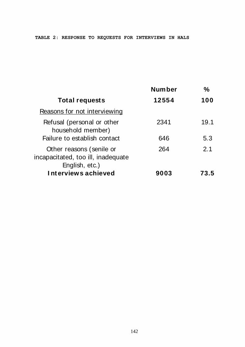
details). This number was relatively small and only 418 addresses were excluded,

leaving a total of 12,254 individuals to be interviewed. The response rate fell more

dramatically when it came to success in completing these interviews. 9,003 interviews

were completed (see Table 2). This is a response rate of 73.5%. In other words, there

was a 1 in 4 chance that an interview was not completed. The missing values are an

example of unit non-response. For these individuals, no information is available from

any of the survey questions. The main reason for non-response is refusal on the part of

the interviewee or their family. This accounted for 2,341 cases or 19% of the requests

for interview. Further cases were lost because the interviewer was unable to establish

contact or for other reasons, such as illness or incapacity on the part of the interviewee.

INSERT TABLE 1

INSERT TABLE 2

A question for researchers is whether the 1 in 4 individuals who were not included in

the survey are systematically different from those who did respond. If there are

systematic differences, this creates a problem of sample selection bias and it will not be

possible to claim that inferences based on the observed data are representative of the

underlying population (see Chapter 7). What do we know about the people who did not

participate in the interview? Although the survey provides no information, we do know

the addresses of the non-responders. This allows us to compare response rates across

geographic areas and to use other sources of information about those areas (see Table

3). For example, analysis of the HALS data shows that response rates were particularly

low in Greater London with a response rate of 64.2% compared to 73.5% on average.

The representativeness of the sample can be gauged further by comparing the observed

data to external data sources. So, for example, the HALS team compared their survey

to the 1981 census (see Table 4). This comparison suggests that the HALS data under-

represent men and over-represent women with only 43.3% of men amongst the

interviewees compared to 47.7% in the census.

INSERT TABLE 3

INSERT TABLE 4

11

The overall response rate of 73.5% is fairly typical of general population surveys.

Understandably, the response rate declines for the subsequent nurse visit and postal

questionnaire. The overall response rate for those individuals who completed all three

stages of the survey is only 53.7%. Comparison with the 1981 census suggests that this

final sample under-represents those with lower incomes and lower levels of education.

It is important to bear unit non-response in mind when doing any analysis with all

survey data sets.

A further source of missing data is item non-response. This occurs when an individual

responds to the interview as a whole but is unwilling or unable to answer a particular

question. Non-responses are coded as “missing values” in the dataset. Again

researchers should be aware of the potential bias this creates if observations with

missing values are systematically different from those who respond to the question. For

example, the self-employed may be less willing to reveal information about their

income than those in paid employment. Chapter 7 discusses some of the methods that

can be used to deal with non-response and the sample selection bias it can create.

2.2 The longitudinal follow-up

The HALS data were originally intended to be a one-off cross-section survey and most

of the examples used in this book are drawn from the original cross-section. However,

HALS also provides an example of a longitudinal or panel data set. In 1991/92, seven

years on from the original survey, the HALS was repeated. This provides an example

of repeated measurements where the same individuals are re-interviewed. Panel data

provide a powerful enhancement of cross-section surveys that allows a deeper analysis

of heterogeneity across individuals and of changes in individual behaviour over time.

However, because of the need to revisit and interview individuals repeatedly the

problems of unit non-response tend to be amplified. Of the original 9,003 individuals

who were interviewed at the time of the first HALS survey 808 (9%) had died by the

time of the second survey, 1,347 (14.9%) could not be traced and 222 were traced but

12

could not be interviewed, either because they had moved overseas or they had moved to

geographic areas that were out of the scope of the survey. These cases are examples of

attrition - individuals who drop out of a longitudinal survey. Systematic differences

between the individuals who stay in and those who drop out can lead to attrition bias.

This is discussed in more detail in Chapter 11.

2.3 The deaths data

HALS provides an example of a cross section survey (HALS1) and panel data

(HALS1&2). Also it provides a longitudinal follow-up of subseqent mortality and

cancer cases among the original respondents. These deaths data can be used for survival

analysis (see Chapter 10). Most of the 9003 individuals interviewed in HALS1, have

been flagged on the NHS Central Register. In June 2005 the fifth death revision and the

second cancer revision were completed. The flagging process was quite lengthy because

it required several checks in order to be sure that the flagging registrations were related

to the person previously interviewed. As reported in Table 5, about the 98 per cent of

the sample has been flagged. Deaths account for some 27 per cent of the original

sample.

INSERT TABLE 5

2.4 Socioeconomic characteristics Most of the empirical models shown in this book use a common set of individual

socioeconomic characteristics as explanatory variables (also know as independent

variables or as regressors). These include examples of continuous regressors, whose

values can be treated as varying continuously (in practice these kinds of variables may

include integer-valued variables that have sufficient variability to be treated as

approximating a continuous variable). The example of a ‘continuous’ variable in our

data is the individual’s age (age) which is measured in years. To allow for a flexible

13

relationship between age and the outcomes of interest squared and cubic terms are

included in the models as well (age2 and age3). Also age is centred around age 45 (the

reason for this is explained below). All of the other regressors are indicator variables

(also know as dummy variables). These take a value 1 if an individual has a particular

characteristic and 0 otherwise. The dummy variables are included in groups. There is a

single indicator for gender (male). Ethnic group is split into black and West Indian,

Indian, Pakistani and Bangladeshi, and other non-white (ethbawi, ethipb, ethothnw).

Employment status covers part-time employed, unemployed, retired, full-time students

and keeping house (part, unemp, retd, stdnt, keephse). Education is measured by the age

that an individual left full-time education: under 14, 14, 15, 17, 18 or over 18 (lsch14u,

lsch14, lsch15, lsch17, lsch18, lsch19). Social class is measured by the Registrar

General’s occupational social class (regsc1s, regsc2, regsc3n, regsc4, regsc5n). Marital

status includes widowed, never married, separated and divorced (widow, single, seprd,

divorce). It should be clear that each of these groups has an omitted category. This is to

avoid the ‘dummy variables trap’ that would create perfect collinearity in the regression

models if a dummy variable was included for every category. The omitted categories

are female, white, employed, left school at 16, social class 3 manual and married and

the reference age is 45. Together these define the ‘reference individual’, a concept that

is discussed in more detail below.

Table 6 shows descriptive statistics, produced using the ‘summarize’ command in Stata,

for the full list of socioeconomic variables. These show that 43 per cent of the sample

are men and the average age is 46, with a range from 18 to 98. There are relatively few

respondents from non-white ethnic minorities represented in the sample. After full-time

employees (the omitted employment category), the retired are the next largest group,

with 22 per cent of the sample. Most respondents left school at age 16 (the omitted

category), followed by 15 and 14. The majority are married (the omitted category)

followed by those who had never married at the time of the survey.

INSERT TABLE 6

14

Appendix: Stata code for data handling and descriptive statistics The HALS data are stored as a Stata dataset. The first step is to load the Stata dataset

into the package. This can be done with the ‘use’ command: use "c:\....\...\your_filename.dta", clear It is helpful to open a log file that will store a permanent record of the output of the

session: log using "c:\...\...\your_filename.log", replace Considerable time and effort can be saved by creating a ‘global’ for the list of variable

names. This avoids having to type them out in full in subsequent commands. Here a

global ‘xvars’ is created that lists all of the socioeconomic variables that will be used in

the regression models: global xvars "male age age2 age3 ethbawi ethipb ethothnw part unemp retd stdnt keephse lsch14u lsch14 lsch15 lsch17 lsch18 lsch19 regsc1s regsc2 regsc3n regsc4 regsc5n widow single seprd divorce partime retired student keephouse"

This global can then be used in the ‘summarize’ command to provide descriptive

statistics for the variables: summ $xvars One way of assessing the importance of non-response is to compare the descriptive

statistics for the sample of observations that are used to estimate the regression model

and the sample of available observations that are not used. Here a regression model for

self-assessed health (sah) is used to create an indicator variable for those observations

that are selected into the sample. A convenient feature of Stata is ‘e(sample)’, an

indicator of whether of not an observation was in the sample used to estimate the

regression model. This is used to create the indicator ‘miss’ so that the descriptive

15

statistics can be calculated separately ‘by’ the values of miss (i.e. for the estimation

sample and for the remaining sample):

gen yvar = sah quietly regr yvar $xvars gen miss=0 recode miss 0=1 if e(sample) sort miss by miss: summ $xvars

16

Chapter 3 Binary Dependent Variables

3.1 Methods

It is often the case in survey data that the outcome of interest is measured as a binary

variable, taking values of either one or zero. Often this binary variable will indicate

whether an individual is a participant or a non-participant. Examples include: health

care utilisation, such as whether an individual has visited a GP in the previous month, or

whether they have used prescription drugs; or whether a household has purchased health

insurance; or whether an individual is a current smoker. If the binary outcome y,

depends on a set of explanatory variables x, then the conditional expectation of y given

x, in other words the value of y that individuals with characteristics x are likely to report

on average, is

E(y | x) = 0.P(y=0|x) + 1.P(y=1|x) = P(y=1 | x) = F(x) (2)

A simple way to model binary data is to use a linear function: for which we can use the

shorthand notation, F(x) = xβ. This gives the linear probability model. The linear

probability model is straightforward to estimate, using standard software for the method

of ordinary least squares.

These estimates should be adjusted for the fact that, by design, the error term in the

equation cannot have a normal distribution. Normality implies that the error is

continuous and can take any value between plus and minus infinity. In the linear

probability model, the error term can take only two values corresponding to values of

zero or one for the dependent variable. The variance of this implied error term depends

on the value of the x’s. In other words, by design, the error term is heteroskedastic

(meaning that its variance differs across individuals with different values of x). This

can be corrected by using a robust estimator of the standard errors, while using

weighted least squares, rather than ordinary least squares, can improve the efficiency

17

of the estimates.

In practice, the linear probability model may provide a reasonable approximation for

binary choice models, so long as the function F(.) is approximately linear over the range

of sample observations. But a major drawback of the method is that, because a straight

line is used, predicted values of the regression function can lie outside the range zero to

one. Equation (2) shows that these predicted values correspond to the probability that

an individual participates. This means that the linear probability model can lead to

logical inconsistencies, with predicted probabilities outside the logical range zero to

one. A way to avoid this is to use a non-linear function for F(.). Popular choices are

“S” curves, that are bounded to the range [0,1] whatever the values of the regressors x.

The most common choices of these “S” curves are logit and probit models.

Logit and probit models are often motivated in terms of a latent variable specification.

This assumes that there is some continuous latent variable y* that determines

participation. You can think of y* as an individual’s propensity to participate. If y* is

positive, the individual will choose to participate and the observed binary outcome

equals 1. Otherwise, the individual will not participate and the observed value equals 0.

Then the latent variable y* is modelled by a linear regression function of the individual

characteristics x. Assuming that the error term in this equation has a standard normal

distribution gives the probit model. Assuming that it has a standard logistic

distribution gives the logit model. The probability functions for the probit and logit

models both have the characteristic “S” shape and are similar in appearance, although

the logit model gives more weight to the tails of the distribution. As with many of the

models described in this book, logit and probit models are typically estimated by the

method of maximum likelihood estimation. This method is discussed in more detail in

the technical appendix.

3.2 Results for the linear probability model

To illustrate the estimation and interpretation of linear probability, logit and probit

18

models, we will use HALS data on individuals’ self-assessed health. In HALS, self-

assessed health is measured on a four point scale with categories “excellent”, “good”,

“fair” and “poor”. To illustrate binary choice models, this is collapsed into a binary

variable where y = 1, if an individual reports excellent or good health, and y = 0, if an

individual reports fair or poor health. The aim is to model the probability of an

individual reporting excellent or good health as a function of a range of socio-economic

characteristics, including the individual’s gender, age, ethnic origin, work status,

educational qualifications, occupational socio-economic group and marital status.

Table 7 presents the weighted least squares estimates for the linear probability model.

These are computed in two steps. First, the model is estimated using ordinary least

squares and the predicted values from this equation are saved. These predictions are

then used to calculate weights. This is possible only if the predictions lie within the

range [0,1]. So, any logically inconsistent predictions mean that it is not possible to use

weighted least squares. In the example reported here, this was not a problem as all of

the predictions are in the required range.

INSERT TABLE 7

One attraction of the linear probability model is its ease of interpretation. As we have

seen in equation (2), the regression function, E(y|x), can be interpreted as the probability

of participating given the values of x, and here this is assumed to be a linear function.

This means that the regression coefficients β are measured in units of probability. So,

for example consider the constant term 0.754 (in the final row of Table 7). This is the

value of the regression function when all of the x variables equal 0. You can think of

this as a “reference individual”. In this example, the x variables have been constructed

so that the reference individual is a woman aged 45 who is white, in full-time

employment, left school at 16, is in a skilled manual occupation and is married. The

coefficient tells us that this type of individual has a probability of 0.754 of reporting

excellent or good health, rather than fair or poor health.

The coefficients on the x variables tell us how this probability changes with changes in

19

the individual’s characteristics. The regression function includes two types of

explanatory variable. The first type can be treated as though they were continuous

variables. The example here is the individual’s age measured in years. All of the other

explanatory variables are binary or dummy variables. These take the value 1 if the

individual has a particular characteristic, for example, if they are unemployed, and 0

otherwise.

An important general tool for interpreting the impact of changes in the regressors on the

probability of participation is the partial effect. The way of calculating the partial effect

depends on whether the regressor is continuous or discrete. For continuous explanatory

variables, we look at the impact of a small change in the variable on the probability of

participation. This is known as the marginal effect. Here we could look at the impact

of age on the probability of reporting excellent or good health. For the dummy

variables, it does not make sense to think in terms of small changes. An individual

either has a characteristic or does not. Here, we look at the average effect, for example

the difference in the probability of reporting excellent or good health if someone is

unemployed compared to someone who is employed.

An attraction of the linear probability model is that the regression coefficients directly

measure both the marginal effect of continuous explanatory variables and the average

effect of dummy explanatory variables.

The sign of the coefficients tells us about the qualitative effect of the explanatory

variables. For example, Table 7 shows that the coefficient on unemployment is

negative (-0.045). This means that an individual who is currently unemployed has a

lower probability of reporting good or excellent health relative to the reference

individual who is employed. The size of the coefficient tells us about the quantitative

effect of the variable. The coefficient on unemployment is –0.045. This is measured in

units of probability and tells us that the probability of reporting good or excellent health

is 0.045 lower for someone who is unemployed than for the reference individual.

We are relying on a point estimate (-0.045) of the impact of unemployment. The fact

20

that this estimate is different from zero may simply be due to chance, attributable to

sampling variability. This sampling variability is summarised by the standard error of

the coefficient. The null hypothesis that the coefficient equals zero can be tested by

looking at the t-ratio; given by the ratio of the coefficient to its standard error. t-ratios

are reported in the fourth column of Table 7 and the corresponding p-value (the implied

significance level of the test) is given in the fifth column. With a t-ratio of –2.06, we

can say that the coefficient on unemployment is statistically significant at a

conventional 5 percent level of significance.

Now consider the other variables included in the model. The qualitative effects for

occupational socio-economic group show that those in social classes 1, 2 and 3 (non-

manual) have positive coefficients. In other words, they are more likely to report good

or excellent health compared to the reference individual who is in social class 3 - skilled

manual occupations. Individuals in social classes 4 and 5 - semi-skilled and unskilled

occupations - have negative coefficients, showing that, on average, they are less likely

to report good or excellent health. The quantitative effects show some evidence of a

gradient in health across socio-economic groups.

A similar pattern emerges for education. Here, the reference category is leaving school

at age 16. The qualitative effects show that those who left school at 15, 14 or under are

less likely to report good or excellent health, while those who left school at 17 or older

are more likely to report good or excellent health.

A further note of caution is that the coefficients on the explanatory variables tell us

about the impact of changing each variable, holding all of the others constant. This

means that the age variables need to be interpreted with care because the model also

includes the square and the cube of age. The fact that the level of age has a negative

coefficient does not mean anything in itself. In other words, it is not possible to

increase age by one year without also changing the values of age-squared and age-

cubed. To understand how self-assessed health changes with age, you would need to

look at the change in all three variables. One way of presenting the results would be to

plot the shape of the fitted polynomial function of age. An alternative approach would

21

be to specify the age profile as a step function: in this case dummy variables could be

used to indicate age ranges, such as 20-25 etc. Then the coefficients would indicate the

impact of each age group relative to a reference age range that is omitted from the

model.

The interpretation of the results so far assumes that the model we are using is well-

specified. For example, choosing the probit model assumes that the function F(.) is the

normal distribution function and that it’s argument is linear in the x variables. This may

not be the case. A convenient way of testing the specification of the model is to use a

regression error specification test (RESET). This is a general test for problems with the

assumed functional form of the model, in particular the assumption of linearity. It is

sometimes used as a test for omitted variables - other explanatory variables that have

not been included in the model and are correlated with both the dependent variable and

with the included explanatory variables – as well. But it will only be an effective

diagnostic for omitted variables if these lead to nonlinearity in the relationship between

y and x.

The RESET test is easy to implement. It involves saving the predicted values from the

regression function, taking the square of those values and re-estimating the model with

this new variable added as an extra explanatory variable (higher order terms, such as the

cubed and quartic of the fitted values, could be added as well. This is the default when

the RESET test is computed automatically in Stata). If the model is well specified this

new test variable should not be significant. If the model is poorly specified the test

variable will be significant. A convenient way of carrying out the test is to look at

either the t-ratio or the F test for the null hypothesis that the coefficient on the new

variable equals zero (note that the t-ratio squared equals the F test). For the linear

probability model of self-assessed health, reported in Table 7, the RESET test gives a F

test statistic of 4.42 (p=0.04). This fails a conventional 5% significance test and the size

of the statistic is a cause for a concern.

3.3 Results for the probit model

22

How do the results for the linear probability model compare to those for the probit and

logit models? Table 8 shows the estimates for the probit model, computed using the

method of maximum likelihood estimation. Like the linear probability model, the table

includes coefficients, their standard errors and z-ratios. The z-ratio is computed in the

same way as the t-ratio, by taking the ratio of the coefficient and the standard error.

Hypothesis testing in models estimated by maximum likelihood has to rely on the

sample size being large enough for the coefficients to follow a normal distribtion (a so-

called asymptotic property). With a large sample size the z-ratio has a standard normal

distribution.

The interpretation of the probit coefficients is different from the linear probability

model. Recall that the probit model takes a linear function of the explanatory variables

and applies a non-linear transformation, in this case using the S-curve of the normal

distribution function. The coefficients relate to the underlying linear index. These are

often interpreted in terms of the latent variable y*. But y* is inherently unobservable

and is not measured in any kind of natural units, unlike the probability of participation.

In themselves, the coefficients should therefore be interpreted only as qualitative

effects. So, for example, a negative coefficient means that somebody is less likely to be

a participant, and a positive coefficient means they are more likely to be a participant.

Unemployment has a coefficient of –0.137 in the probit model. This cannot be

compared directly to the coefficient from the linear probability model. The qualitative

interpretation is that, due to the negative coefficient, the unemployed are less likely to

report good or excellent health. Similarly, the qualitative results show that those in

professional and managerial occupations are more likely to report good or excellent

health, while those in semi-skilled and unskilled occupations are less likely to report

good or excellent health. Also, those with more education are more likely to report

good health and those with fewer years of education are less likely (with the possible

exception of those who left school at age 19 or more).

INSERT TABLE 8

In order to interpret the quantitative implications of the results we need to compute

23

partial effects, using marginal effects for continuous explanatory variables and average

effects for binary explanatory variables. Unlike the linear probability model, the

marginal or average effects are not given by the coefficients directly but they can be

computed from them. The formula for the marginal effect of an explanatory variable xk

is,

∂P(y=1|x)/∂xk = βkf(xβ) (3)

where f(.) = ∂F(.)/∂(xβ). The formula for the average effect of a binary variable is,

P(y=1| xk =1) - P(y=1| xk =0) = F(xβ| xk =1) - F(xβ| xk =0) (4)

These are more complex formulas than the linear probability model due to the non-

linearity of the F(.) curve. Also, it should be clear that both the marginal and average

effects depend on the values of the x variables. In other words, they are different for

different types of individual. The size of the effect of a variable, say unemployment,

will depend on the value of the other explanatory variables, such as education, marital

status and age. One common way of dealing with this is to evaluate the effect at the

sample mean of the other x variables, treating this as a “typical” observation. This is

the approach adopted in software packages such as Limdep and Stata. However, this

can be a rather artificial approach, especially when the x’s include dummy variables, as

the typical observation is unlikely to correspond to any actual observation. An

alternative is to compute the effect for each observation, using their specific x-values,

and then report summary statistics such at the sample mean of the effects: this is known

as the average partial effect (APE).

INSERT TABLE 9

Table 9 presents the average and marginal effects for the probit model as computed

automatically by the dprobit command in Stata. The effects in Table 9 can be given a

quantitative interpretation and are measured in units of probability. Consider the impact

of unemployment. Here the average effect is –0.047, which is very similar to the

estimate of –0.045 of the linear probability model (see Table 7). It tells us that the

24

probability of an unemployed person reporting good or excellent health is 0.047 less

than an full-time employed person (at the average value of the other regressors). In this

case, the estimated effect of unemployment is quite similar across the linear probability

and probit specifications. However, comparing the estimates for other explanatory

variables shows that this is not always the case. For example, the average effect of

being in part-time, rather than full-time, work is 0.053 in the probit model (Table 9)

compared with 0.064 in the linear probability model (Table 7). One note of caution is

that the automated computation of partial effects provided by the dprobit command may

produce misleading results. Table 9 displays separate marginal effects for age, age-

squared and age-cubed, treating them as separate variables. But, of course, it is not

possible to change one of these variables without changing the other two. The correct

approach would be to compute the overall derivative with respect to age. A similar issue

arises when interaction terms between different regressors are included in the model and

again derivatives should be computed directly.

Finally, Table 9 presents the RESET test for the probit model. Unlike the linear

probability model, there is no evidence of misspecification and the chi-squared statistic

for the test is 0.27 with a p-value well above conventional significance levels (p=0.603).

3.4 Results for the logit model

Tables 10 and 11 present the coefficient estimates and average and marginal effects for

a logit model of self-assessed health. Here, the standard normal distribution of the

probit model is replaced by a standard logistic function. Once again, the coefficients can

be given a qualitative interpretation and these qualitative effects follow the same pattern

as the probit model. In the logit model the β coefficients can be interpreted in terms of

log-odds ratios, a concept that is commonly used in biostatistics and epidemiology.

Because of the particular functional form of the standard logistic distribution the odds

ratio simplifies to P(yj=1)/P(yi=0) = exp(xβj) and therefore the coefficients can be

interpreted in terms of changes in the log-odds-ratio log(P(yj=1)/P(yi=0)).

25

The marginal and average effects show the quantitative impact and these can be

compared directly to the linear probability and probit estimates. So, for example, the

average effect of unemployment in the logit model is -0.046 (Table11) compared with –

0.047 for the probit model (Table 9) and –0.045 for the linear probability model (Table

7). The logit model also passes a RESET test with a chi-squared statistic of 0.08

(p=0.783).

INSERT TABLE 10

INSERT TABLE 11

26

Appendix: Stata code for binary choice models

Linear probability model

The basic linear probability model can be estimated by ordinary least squares (OLS)

using the ‘regress’ command. Robust standard errors are used. Also the ‘predict’

command is used to save the fitted values from the linear regression as a new variable

called ‘yf’: regress yvar $xvars, robust predict yf

For comparison with the probit and logit models it is useful to save and rename the

coefficients. Here the coefficient on ‘unemp’ is singled-out and saved as a scalar

‘bun_lpm’: matrix blpm=e(b) matrix list blpm scalar bun_lpm=_b[unemp] scalar list bun_lpm

The fitted values, saved above as the new variable ‘yf’, can be used to create the

weights that are needed to adjust for the heteroskedasticity that is inherent in the linear

probability model. Then the ‘aweight’ option can be used to run weighted least squares

(WLS): * WEIGHTED LEAST SQUARES gen wt=1/(yf*(1-yf)) regress yvar $xvars [aweight=wt]

The fitted values can be squared and added back to the original regression model in

order to compute the RESET test for misspecification of the model. Here we are only

interested in the t-ratio for the new variable ‘yf2’ so the rest of the regression output is

suppressed using the ‘quietly’ option:

* RESET TEST gen yf2=yf^2 quietly regress yvar $xvars yf2, robust

27

test yf2=0 Probit model

The syntax for the probit model is very similar to the linear regression, with ‘regress’

replaced by ‘probit’. Fitted values can be saved for the linear index, xβ, using ‘predict’:

probit yvar $xvars predict yf, xb Stata provides a command, ‘dprobit’, that automatically presents the results as partial

effects, calculated at the sample means of the regressors:

dprobit yvar $xvars

Again we can save the beta coefficients and, in this case, also rescale them so that they

are comparable to the LPM. There are two options discussed in the literature, rescaling

by 1.6 or by 1.8. The code does both:

matrix bpbt=e(b) matrix list bpbt scalar bun_pbt=_b[unemp] scalar bun_pbt18=_b[unemp]*1.8 scalar bun_pbt16=_b[unemp]*1.6 scalar list bun_pbt bun_pbt18 bun_pbt16

Rather than calculating partial effects at the sample means of the regressors (as in

‘dprobit’) it is preferable to compute them using the actual x-values for each

observation. The formulas for the marginal effect of a continuous variable and the

average effect of a discrete variable can be computed directly:

* MARGINAL EFFECTS gen mepbt_unemp=bun_pbt*normden(yf) * AVERAGE EFFECTS gen aepbt_unemp=0 replace aepbt_unemp=norm(yf+bun_pbt)-norm(yf) if unemp==0 replace aepbt_unemp=norm(yf)-norm(yf-bun_pbt) if unemp==1

28

Once these have been computed ‘summ’ can be used to compute the average partial

effects and other descriptive statistics. A histogram of the partial effects could be

plotted using ‘hist’ to give a sense of the overall distribution of the effects:

summ mepbt_unemp aepbt_unemp hist aepbt_unemp

The format for the RESET test mirrors the code used for the LPM:

gen yf2=yf^2 quietly probit yvar $xvars yf2 test yf2=0 Logit model

Most of the code needed for the logit model is analogous to the probit. There is no

equivalent to ‘dprobit’ so the slower command ‘mfx’ has to be used. The expessions for

the direct computation of the partial effects use the logistic distribution rather than the

standard normal distribution:

logit yvar $xvars mfx compute if e(sample) predict yf, xb * SAVE COEFFICIENTS matrix blgt=e(b) matrix list blgt scalar bun_lgt=_b[unemp] scalar list bun_lgt bun_pbt18 bun_pbt16 * MARGINAL EFFECTS gen melgt_unemp=bun_lgt*( exp(yf)/(1+exp(yf)))*(1-exp(yf)/(1+exp(yf))) * AVERAGE EFFECTS gen aelgt_unemp=0 replace aelgt_unemp=exp(yf+bun_lgt)/(1+exp(yf+bun_lgt))-exp(yf)/(1+exp(yf)) if unemp==0 replace aelgt_unemp=exp(yf)/(1+exp(yf))-exp(yf-bun_lgt)/(1+exp(yf-bun_lgt)) if unemp==1 summ mepbt_unemp aepbt_unemp melgt_unemp aelgt_unemp scalar list bun_lpm * RESET TEST gen yf2=yf^2 quietly logit yvar $xvars yf2 test yf2=0

29

Chapter 4 The Ordered Probit Model

4.1 Methods

The empirical example in the previous section uses a binary measure of self-assessed

health. This variable was created artificially by collapsing the underlying 4-category

scale where health could be assessed as either excellent, good, fair or poor. This is an

example of a categorical variable where respondents are asked to report a particular

category and where there is a natural ordering. It seems reasonable to assume that

excellent health is better than good, which is better than fair, which is better than poor,

for everyone in the population. An econometric model that can be used to deal with

ordered categorical variables is the ordered probit model. This is designed to model a

discrete dependent variable that takes ordered multinomial outcomes. For example, y =

0,1,2,3,..... It should be stressed that y is measured on an ordinal scale and the

numerical values of y are arbitrary, except that they must be in ascending order.

The ordered probit model is an extension of the binary probit model (a similar extension

is available for the logit model). Like the binary probit model, the ordered probit model

can be expressed in terms of an underlying latent variable y*. Here this could be

interpreted as the individual’s “true health”. The higher the value of y*, the more likely

they are to report a higher category of self-assessed health. In our case there are four

categories, so the range of values y* should be divided into four intervals, each one

corresponding to a different category of self-assessed health. The threshold values (µ)

correspond to the cut-offs where an individual moves from reporting one category of

self-assessed health to another. It is not possible to identify both the constant term and

all of the cut-off points. So, in order to estimate the model, some of the threshold values

(µ’s) have to be fixed. The lowest value is set at minus infinity, the highest value is set

at plus infinity and one other value has to be fixed. Conventionally, either the upper

bound of the first interval (µ1) is set equal to zero or the constant term is excluded from

the regression model. Like the binary probit model, explanatory variables are

30

introduced into the model by making the latent variable y* a linear function of the X’s,

and adding a normally distributed error term. This means that the probability of an

individual reporting a particular value of y=j is given by the difference between the

probability of the respondent having a value of y* less than µj and the probability of

having a value of y* less than µj-1. Using these probabilities it is possible to use

maximum likelihood estimation to estimate the parameters of the model. These include

the βs (the coefficients on the X variables) and the unknown cut-off values (the µs).

The ordered probit model applies when the threshold values (µ) are unknown. A variant

on the model is grouped data regression or interval regression. This can be used when

the values of thresholds are observed. For example, in many health interview surveys,

including HALS, individuals are presented with a range of categories and asked to state

where their income lies. These categories are selected by the researcher and the upper

and lower thresholds are known. Because the value of the µ’s are known and do not

have to be estimated, the estimates of the coefficients on the explanatory variables are

more efficient. Also, because the values of the thresholds are in natural units, such as

money, the predicted values from the grouped data regression are also measured in

those units. This means that the grouped data regression is able to estimate the variance

of the error term (σ2) as well as the β’s. What is more, this scaling means that the latent

variable is also measured in natural units and hence the coefficients measure marginal

or average effects in natural units.

4.2 An application to self-assessed health

To illustrate the use of the ordered probit model, Table 12 shows estimates for the four-

category measure of self-assessed health. The dependent variable is coded 0 for poor

health, 1 for fair health, 2 for good health and 3 for excellent health. Table 12 includes

the coefficients, their standard errors and z-ratios. It also includes estimates of the

threshold parameters µ1, µ2 and µ3 (the default in Stata is to exclude the constant term

in order to identify model). These imply that a value of the latent variable less than –

31

1.717 corresponds to poor health, a value between -1.717 and –0.641 corresponds to fair

health, a value between –0.641 and 0.783 corresponds to good health and a value above

0.783 corresponds to excellent health. Notice that the predicted value of y* for the

reference individual, where all of the explanatory variables equal zero, is zero. This

value lies between –0.641 and 0.783, hence the reference individual would be predicted

to report good health.

INSERT TABLE 12

As for the binary probit model, the coefficients on the explanatory variables have a

qualitative interpretation. A positive coefficient means that an individual has a higher

value of latent health and is more likely to report a higher category of self-assessed

health. A negative value means that they have a lower value of the latent variable and

are likely to report a lower category of self-assessed health. As before, the results show

a socio-economic gradient in self-assessed health. Those in professional and

managerial occupational groups have positive coefficients, those in semi-skilled and

unskilled occupations have negative coefficients. A similar gradient is apparent for

levels of education. Because the threshold values are unknown, the latent variable and

hence the coefficients are not measured in natural units. Like the binary probit model,

quantitative predictions should be made on the basis of marginal effects for continuous

explanatory variables and average effects for binary explanatory variables.

Once again, it is important to test the specification of the model before putting too much

weight on the results. In fact a RESET test suggests that the model is mis-specified, the

chi-squared is 5.20 (p=0.023). This suggests that more work needs to be done to

improve the specification of the model, perhaps by changing the way in which the

explanatory variables are measured by finding additional explanatory variables, or by

splitting the sample into separate groups, perhaps by gender, or using a distribution

other than the standard normal.

32

Appendix: Stata code for the ordered probit model The basic syntax for running an ordered probit model, with an option to tablulate the

actual and fitted values is given below. Predictions of the linear index are saved for

future use:

oprobit yvar $xvars, table predict yf, xb With the ordered probit model, partial effects can be computed for each of the observed

values of y. Here the partial effects for P(y=0) are computed. An automated version is

available with the ‘mfx’ command (based on evaluating at the means of the regressors):

mfx compute, predict(outcome(0))

Or the partial effects can be computed for each observation. The formula for the average

effect of ‘unemp’ involves the estimated cut-points, saved as scalars _b[cut1] etc, as

well as the beta coefficients:

scalar mu1=_b[_cut1] scalar bunemp=_b[unemp] gen aeop_unemp=0 replace aeop_unemp=norm(mu1-yf-bunemp)-norm(mu1-yf) if unemp==0 replace aeop_unemp=norm(mu1-yf)-norm(mu1-yf+bunemp) if unemp==1 summ aeop_unemp hist aeop_unemp The RESET test follows the by now familiar format: gen yf2=yf^2 quietly oprobit yvar $xvars yf2 test yf2=0 drop yf yf2

33

Chapter 5 Multinomial Models

5.1 The multinomial logit model

The ordered probit model discussed in the previous section applies to ordered

categorical variables. Multinomial models apply to discrete dependent variables that

can take unordered multinomial outcomes, for example, y = 0,1,2,3,..... that represent a

set of mutually exclusive choices. Again, the numerical values of y are arbitrary and in

this case they do not imply any natural ordering of the outcomes. A classic example in

economics is “modal choice” in transport. Here, the outcomes could represent different

modes of transport, for example, plane, train, car, and the individual faces a choice of

one of these mutually exclusive modes of transport. This choice will depend on

characteristics of the alternatives, such price, convenience, quality of service and so on,

and the characteristics of individuals, such as their level of income. Some of the

characteristics of the alternatives, such as distance to the nearest hospital, may vary

across individuals as well. There is unlikely to be a natural ordering of the choices that

applies to all individuals in all situations. In health economics, multinomial models are

often applied to the choice of health insurance plan or of health care provider. They

could also be used to model a choice of a particular treatment regime for an individual

patient.

The most commonly applied model is the mixed logit model which is a natural

extension of the binary logit model. In the mixed logit model, the probability of

individual i choosing outcome j, is given by,

Pij = exp(xiβj + zijγ) / ∑k exp(xiβk+ zikγ) (5)

Notice that the coefficients (βj) on the explanatory variables that vary across individuals

(xi) are allowed to vary across the choices, j. So, for example, the impact of income

could be different for different types of health care provider. The coefficients (γ) on the

34

variables that vary across the choices, and perhaps also across individuals (zij) are

constant. So, for example, there may be a common price effect of the choice of

provider. The mixed logit nests two special cases: the multinomial logit or

“characteristics of the chooser” model, when all of the γ equal zero; and the conditional

logit or “characteristics of the choices” model, when all of the βj equal zero. It is worth

noting that the label mixed logit is sometimes applied to the more comples random

parameters logit model which is not discussed here.

Focusing on the multinomial logit model, it is not possible to identify separate βs for all

of the choices. To deal with this it is conventional to set the βs for one of the outcomes

equal to zero. This normalisation reflects the fact that only relative probabilities can be

identified with respect to some base-line alternative. For example, in a model of

hospital utilisation, where the possible outcomes are:

• no-use of hospital services;

• use of hospital outpatient services only;

• use of hospital inpatient services and/or outpatient services;

no-use may be treated as the base-line category. The multinomial logit model would

identify the probability of using outpatient services relative to no use and the probability

of using inpatient services relative to no-use.

The mixed logit model is well-established and widely available in computer software

packages. However, it is a restrictive specification and, in particular, it implies the

“independence of irrelevant alternatives” (IIA) property. To see this, consider the ratio

of the probabilities of choosing two specific alternatives, j and l,

Pij/Pil = [exp(xiβj+ zijγ) / ∑k exp(xiβk+ zikγ)]/[exp(xiβl+ zilγ) / ∑k exp(xiβk+ zikγ)] = exp(xiβj+ zijγ)/exp(xiβl+ zilγ) (6)

This shows that the relative probability only depends on the coefficients and

characteristics of the two choices - j and l - and not on any of the other choices

available. This implies that if a new alternative is introduced all of the absolute

probabilities will be reduced proportionately. For example, consider the case of an

35

individual choosing between a branded drug (brand X) and a generic alternative

(generic A). Let us say that, faced with this choice, the probability of choosing brand X

is 0.5 and the probability of choosing generic A is 0.5. The relative probability is

therefore 0.5/0.5 = 1. Now we introduce a third alternative, a new generic B that

shares the same characteristics as generic A. If the two generic drugs are perfect

substitutes for each other, we might expect that the probability of choosing brand X will

remain 0.5 and the probability of choosing each of the generic will be reduced to 0.25

each. But this contradicts the independence of irrelevant alternatives property, as the

relative probability of choosing brand X compared to generic A will be increased to

0.5/0.25 = 2. In order to satisfy the property, all of the absolute probabilities need to

change so that all equal 0.333 and the relative probabilities remain constant. Many

authors argue that the IIA property is too restrictive for many applications of

multinomial models. The IIA property can be relaxed by using various more general

alternatives: such as the nested multinomial logit, the mixed or random parameters logit

or the multinomial probit specification (see Jones (2000) and Train (2003) for further

details).

It is possible to use the mixed logit model to test whether the IIA property is

appropriate. This test will work with three or more alternatives. The basic idea is to

estimate the model with all of the alternatives and then to re-estimate it dropping one or

more of the alternatives. The estimated coefficients should not change when an

alternative is dropped and so a comparison of the two sets of results can be used to test

for the property. This is based on a Hausman test for whether there is a significant

difference between two sets of coefficients: one set that are efficient under the null (IIA

holds) but inconsistent under the alternative (IIA does not hold) and another set that are

inefficient under the null but still consistent under the alternative. In this case the first

set of coefficients would be taken from the model with all the alternatives included, the

second from the model with an alternative excluded.

5.2 An application

36

The mixed logit model only applies when there are a set of mutually exclusive and

exhaustive outcomes. For this application we use the data on health care utilisation that

was added to the questionnaire at the second wave of the survey (HALS2). The HALS

data on health care utilization has to be recoded to satisfy the conditions of mutually

exclusive and exhaustive outcomes. Here a new variable is created that has three

outcomes: no use of health care (y=0); a GP visit but no use of hospital visits, whether

inpatient or outpatient (y=1); a hospital visit, with or without a GP visit (y=2). Results

for the multinomial logit model applied to this dependent variable are shown in Table

13. These include the socioeconomic variables, measured at HALS2, as regressors. Note

that the model includes the usual list of regressors, which does not have explicit

measures of morbidity. The impact of morbidity on the use of health care is likely to be

picked up by age and gender (which are strongly statistically significant in the model)

and to some extent by socioeconomic characteristics that are linked to health.

INSERT TABLE 13

To identify the coefficients of the multinomial logit model one of the outcomes has to

be fixed as a reference point. All of the results should be interpreted relative to this

reference outcome (by default in Stata this is the case of y=0). So they tell us about the

relative probability of having a GP visit (y=1) or a hospital visit (y=2) rather than

having no visit. The β coefficients can be interpreted in terms of log-odds ratios. Given

the normalising restriction that β0=0 which is required to identify the model, then the

odds ratio simplifies to P(yj=1)/P(y0=1) = exp(xβj) and therefore the coefficients can be

interpreted in terms of changes in the log-odds-ratio log(P(yj=1)/P(y0=1)). The

qualitative interpretation of the coefficients depends on their signs. So, for example,

male – with a negative sign in both equations – implies that men are less likely to use

GPs (y=1) than to have no visits (y=0) and are less likely to have a hospital visit (y=2)

than to have no visits. Overall the coefficients on the variables other than age and

gender tend not to be statistically significant, but it would be important to test them in

groups, for example, for marital status as a whole.

37

Appendix: Stata code for the multinomial logit model

The multinomial logit model only applies when there are a set of mutually exclusive

and exhaustive outcomes. The HALS data on health care utilization has to be recoded to

satisfy these conditions. Here a new variable ‘use’ is created that has three outcomes: no

use of health care (y=0); a GP visit but no use of hospital visits, whether inpatient or

outpatient (y=1); a hospital visit, with or without a GP visit (y=2). The command takes

account of missing values which are coded as ‘.’ in Stata: gen hosp=hospop==1 | hospip==1 gen use = 0 replace use=1 if visitgp==1 & hosp==0 replace use=2 if hosp==1 replace use=. if visitgp==. replace yvar=use Estimates of the multinomial logit model can be obtained from the ‘mlogit’ command:

mlogit yvar $xvars

To check whether the independence of irrelevant alternatives (IIA) property holds it is

possible to run a Hausman test procedure. This compares the general model estimated

above with a restricted model in which one of the categories (y=2 in this case) is

dropped: * Hausman test of IIA est store hall mlogit yvar $xvars if yvar!=2 est store hpartial hausman hpartial hall, alleqs constant The same routine could be run again dropping other alternatives.

38

Chapter 6 The Bivariate Probit Model

6.1 Methods

The ordered and multinomial models discussed in the previous two sections deal with

dependent variables that can have different categorical outcomes. However, in both

cases, there is a single underlying outcome variable. In contrast, the bivariate probit

model provides a way of dealing with two separate binary dependent variables.

Essentially it takes two independent binary probit models and estimates them together,

allowing for a correlation between the error term of the two equations. The practical

application discussed here uses the HALS data to estimate the probability of someone

reporting “good” or “excellent” self-assessed health together with the probability of

them being a current smoker. Allowing for correlation between the error terms of the

two equations recognises that there may be unobservable characteristics of individuals

that influence both whether they smoke and their self-assessed health.

Given that the bivariate probit model is a natural extension of the binary probit model, it

is possible to think about the bivariate model in terms of two latent variables, say, y*1

and y*2. Each of the latent variables is assumed to be a linear function of a set of

explanatory variables, which may or may not be the same for the two equations, and

each equation contains an error term. Like the binary probit model, these error terms

are assumed to be normally distributed but they come from a joint or bivariate normal

distribution. The bivariate distribution allows for a non-zero correlation between the

errors. In other words, it is not assumed that the two error terms are independent of

each other.

With two binary variables four possible outcomes can be observed. In the example

here, these are a smoker who reports good or excellent health, a smoker who reports

poor or fair health, a non-smoker who reports good or excellent health, or a non-smoker

who reports fair or poor health. These correspond to different values of the latent

variables y*1 and y*2 (remember that y* is positive for a participant and non-positive

39

for a non-participant). Using the assumption that the error terms are bivariate normal, it

is possible to write down the probability of each of these four outcomes as a function of

the explanatory variables and the unknown parameters of the model. This allows the

model to be estimated by maximum likelihood methods. Because the outcomes are

estimated jointly, it is possible not only to identify the slope coefficients for each of the

two sets of explanatory variables but also the coefficient of correlation between the two

error terms (ρ).

As with the binary probit model, the latent variables - and hence the β’s - are not

measured in natural units and can only be given a qualitative interpretation but, like the

binary probit model, marginal and average effects can be calculated. There is now a

range of options for interpreting the results. Firstly, the same formulas as used for the

binary probit marginal and average effects can be used for the bivariate probit. This

gives the impact of a change of one of the explanatory variables on the marginal

probability of each outcome, for example, the probability of someone being a smoker,

or the probability of someone being in good or excellent health. Secondly, it is possible

to calculate the marginal effect of an explanatory variable on the joint probability of

each of the four outcome combinations, for example the probability that an individual is

both a smoker and in good or excellent health. Finally, it is possible to calculate the

marginal effects of the explanatory variables on conditional probabilities, for example

the probability that someone reports good or excellent health, given that they are a

smoker.

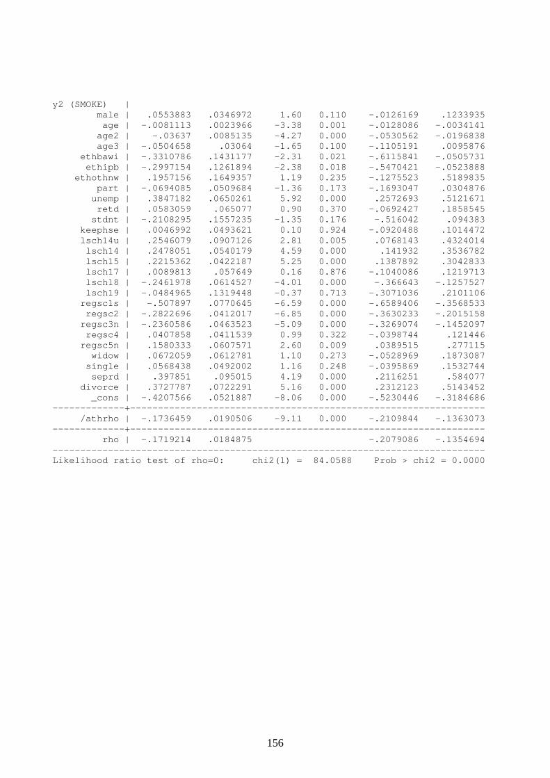
6.2 An application to smoking and health

Table 14 shows the results for the bivariate probit model of smoking and self-assessed

health estimated using the same set of explanatory variables as before. The coefficient

estimates for both equations are broadly similar to those obtained using binary probit

models. The equation for regular smoking shows that those in professional and

managerial socio-economic groups are less likely to be smokers, while those in

unskilled manual occupations are more likely to be smokers. Similarly, those who left

school at 18 are less likely to be smokers, while those who left school before 16 are

40

more likely to be smokers. The socio-economic gradient is once again apparent for self-

assessed health with those in professional and managerial occupations more likely to

report good or excellent health and those in unskilled and semi-skilled occupations less

likely to report good or excellent health. The new information provided by the bivariate

probit model is the estimate of ρ, the correlation coefficient for the two error terms. The

estimate is -0.172 and the chi-squared test of 84.06 shows that this estimate is

significantly different from zero. This is a plausible result that indicates that

unobservable factors that are positively related to smoking are negatively related to

good health.

INSERT TABLE 14

41

Appendix: Stata code for the bivariate probit model

The bivariate probit model requires two binary dependent variables. Here we use

indicators of regular smoking (‘regfag’) and of excellent or good self-assessed health

(‘sah’): gen yvar1=regfag gen yvar2=sah The simple form of the model uses the same set of regressors in both equations.

Predictions of the linear index are saved for each equation:

biprobit yvar1 yvar2 $xvars predict yf1, xb1 predict yf2, xb2

Partial effects can be computed for the marginal, conditional and joint distributions. To

illustrate, the following code computes the average effect of ‘unemp’ on the marginal

probability, p(regfag=1). The results are summarized and displayed in a histogram:

scalar bun_pbt=_b[yvar1:unemp] gen aepbt_unemp=0 replace aepbt_unemp=norm(yf1+bun_pbt)-norm(yf1) if unemp==0 replace aepbt_unemp=norm(yf1)-norm(yf1-bun_pbt) if unemp==1 summ aepbt_unemp hist aepbt_unemp

42

Chapter 7 The Selection Problem

7.1 Identification

Sample selection bias arises when there are missing data for the dependent variable of

interest. Recall the discussion of item non-response in the introduction. For example,

in the HALS data set, measures of physiological health were collected at the nurse visit

but not all of the original interviewees agreed to participate in the nurse visit. Models of

measured health outcomes (for example, forced expiratory volume, fev) could be

estimated on the sample of individuals who responded to the nurse visit. But the

selection problem means that it may not be possible to make inferences about the

determinants of health outcome in the population as a whole. If there are systematic

differences between the type of individuals who respond and those who do not, analysts

are faced by a fundamental problem of identification.

For each individual in the HALS dataset, we know whether or not they responded to the

nurse visit, and we know the characteristics of those who responded and those who

didn’t. Also we have a measure of the health outcome for those who responded and

their associated characteristics. This means we could estimate the probability of

responding, conditional on the explanatory variables, and we can estimate the expected

value of fev, conditional upon the characteristics and on the fact that the individual

agreed to participate. The identification problem arises because there is no way of

knowing the fev score that would have been reported by any individual who refused to

participate in the nurse visit. They could have reported any logically feasible value of

fev. The fact that it is not possible to observe the outcome of the non-responders means

that in general, it is not possible to identify the expected value of the outcome in the

population as a whole. In other words, it is not possible to identify the population

regression function, E(y|x).

At a fundamental level this identification problem is insurmountable. However,

inferences can be made if the analyst is willing to impose some assumptions on their

43

model and data. Traditionally, the statistical literature often assumes independence or

ignorable non-response. This is a strong assumption that asserts that those individuals

who do not respond would behave in the same way as those who do respond,

conditional upon the observed explanatory variables. Given this assumption, estimates

can be adjusted for non-response using inverse probability weights, a method that is

discussed in more detail in Chapters 8 and 11.

Not only is ignorability a strong assumption, it is not possible to test its validity. In the

kind of observational health surveys often used in health economics it is often likely to

be untenable. For example, the reasons why an individual decides not to participate in

the nurse visit may be correlated with unobservable factors that also influence their

health outcome. This would violate the assumption of ignorable non-response and lead

to potential selection bias. Participating in the nurse visit is time consuming and it may

be that those who suspect they may benefit more from the visit, due to pre-existing

chronic conditions, may be more willing to take part. Of course, this also means that

their health outcomes are likely to be poorer than those who are not willing to

participate.

The selection problem can be dealt with if the analyst is willing to impose identifying

restrictions on their model. This involves making assumptions about the functional

form of the regression model, possibly excluding some explanatory variables that

predict non-response from the equations that predict the outcome variable, and also

assumptions about the distribution of the error terms in the two equations. In the

econometrics literature the traditional approach to the selection problem has been a

parametric approach, based on the so-called Heckit model, first introduced by James

Heckman (see e.g., Heckman, 1979). This uses linear regression equations and assumes

that the error terms have a normal distribution. However, recent years have seen the

development of less restrictive semi-parametric estimators which relax some, though

not all, of the identifying restrictions (see Jones, 2000).

44

7.2 The Heckit model

The sample selection model consists of two equations. The first is a probit-type

equation that predicts whether or not somebody responds. The second is a linear

regression equation conditional on the individual providing a response. If it is assumed

that the error terms of the two equations come from a bivariate normal distribution,

which allows for a correlation between the two error terms and therefore the possibility

of sample selection bias, the model can be estimated by maximum likelihood

estimation.

In practice, the model is often estimated by a simpler two-step procedure. The first step

is to estimate a probit equation for non-response and to save the inverse Mills ratio.

The inverse Mills ratio is then added as an extra variable in the second stage regression

of the outcome y on the set of explanatory variables. This second regression is

estimated on the sub-sample of useable responses. Identification of the Heckit model

can rely on finding some explanatory variables that enter the probit equation but do not

enter the second stage regression. In the example given here, these are variables that

influence whether somebody is willing to participate in the nurse visit, but do not

influence their health outcome. In practice, it is often difficult to find such plausible

identification restrictions, in which case the Heckit model is sometimes estimated with

the same set of regressors in each equation. Then, identification relies on the non-

linearity of the inverse Mills ratio. It is worth mentioning that a test of whether the

coefficient of the inverse Mills ratio in the second stage regression is significantly

different from zero, also provides a test for the existence of sample selection bias. This

test is given by the t-ratio associated with the inverse Mills ratio – a large value

provides evidence of selection bias.

In practice, relying on identification by functional form can be problematic. A plot of

the inverse Mills ratio shows that it is approximately linear for much of its range. The

inverse Mills ratio is a function of the linear index (Xβ) from the probit equation. This

means that the range of the linear index, and hence of the explanatory variables in the

probit equation, is important. It also means that the degree of censoring - in other

45

words, the proportion of non-responders in the sample - is important, as this reduces the

range of the observed values of the linear index. The performance of the sample

selection model depends on the collinearity between the inverse Mills ratio and the

explanatory variables in the regression equation. Collinearity is likely to be high if

there are few or no regressors excluded from the second-stage regression, there is a high

degree of non-response, there is low variability among the regressors in the probit

equation or there is a large degree of unexplained variation in the probit equation. So it

is advisable to check for collinearity. A simple way of doing this is to regress the

inverse Mills ratio on the explanatory variables from the outcome equation and examine

the goodness of fit of this equation. A high degree of goodness of fit indicates a high

degree of collinearity.

7.3 An application to data from the nurse visit

One of the measures of physiological health collected at the nurse visit stage of HALS

is the highest forced expiratory volume in one second (‘hyfev’): a measure of lung

capacity. Data on hyfev are only available for those who completed the nurse visit and,

as we saw in Chapter 2, there is non-response at that stage of the survey. This gives us

observations where there is item non-response on the outcome of interest but where we

observe the respondents socioeconomic characteristics that were collected at the face-to-

face interview (i.e. the x’s are not missing). In this case 2,258 observations are missing

for hyfev out of the sample of 9,003.

INSERT TABLE 15

To illustrate the sample selection model we estimate a Heckit model for hyfev, using the

usual set of socioeconomic variables, to see if there is evidence of selection bias. Table

15 shows the full-information maximum likelihood (FIML) estimates of the model,

based on estimating the joint model for both the selection equation and the outcome

equation. The upper panel of results, labelled “y”, is the outcome equation for hyfev, the

second panel, labelled “select” is the probit equation for selection. Here the model is

46

estimated without exclusion restrictions, so the same set of regressors appear in both

equations. In this case the estimated correlation coefficient (‘rho’) is not statistically

significant and the LR test does not reject independence of the two error terms. This

suggests that selection bias is not a problem for the model estimated. However a plot of

the inverse Mills ratio (see Figure 1) shows that there is very little nonlinearity for the

sample used here and identification of the model is likely to be tenuous. Notice the

strong effects of gender and age in the model for hyfev. Subsequent analysis might split

the sample by gender and refine the specification of the age effects, or alternatively

include interactions between age and gender and, perhaps, between gender and other

variables.

INSERT FIGURE 1

The results of the selection part of the model show that, on average and holding other

factors constant, men and part-time workers are significantly more likely to have

responded to the nurse visit. Older people, ethnic minorities, those who had never

married and those from lower socioeconomic groups are less likely to have responded.

47

Appendix: Stata code for the sample selection model

The Sample Selection model (SSM/Heckman selection model/Generalised Tobit model)

can be obtained using the full information maximum likelihood estimator (FIML):

heckman yvar $xvars, select($xvars)

Alternatively the Heckman two-step consistent estimates can be used, with an option to

save the inverse Mills ratio as a new variable ‘imr’:

heckman yvar $xvars, select($xvars) twostep mills(imr)

Here the model is estimated without exclusion restrictions, so that the same set of x-

variables appear in the selection equation and the outcome equation. The shape of the

inverse Mills ratio for the relevant range of the data can be plotted against the linear

index:

probit regfag $xvars predict yfp, xb twoway scatter imr yfp

Also ‘imr’ can be regressed on the x variables to gauge the degree of collinearity:

regress imr $xvars

48

Chapter 8 Endogenous Regressors: the evaluation problem revisited 8.1 The problem restated

Chapter 1 introduced an example of the evaluation problem: how to estimate the

“treatment effect” of ownership of private insurance on the use of health care. From a

policy point of view it is of critical importance to know whether, and to what extent, an

observed association between insurance and utilisation is due to selection effects or to a

direct utilisation effect or both. If the observed insurance effect is entirely due to self-

selection of those more likely to use health care, then private insurance coverage merely

acts as a marker for such propensity and reducing private insurance options will not

reduce the use of care. If, on the other hand, the insurance effect is mostly due to the

utilisation effect of increased coverage, then the expansion or reduction of private

insurance options will have an impact on use.

Therefore, a central question is whether access to private insurance encourages greater

utilisation or not. This may be due to price effects (“moral hazard”), risk reduction

effects, access effects or income-transfer effects. All of these factors may encourage

greater utilisation and they will be referred to collectively as the insurance effect on

utilisation. For example, in a system where private insurance provides supplementary

cover alongside a universal public system - that offers a basic package of services that

are free at the point of use - the access effect may be the prime reason for increased

utilisation among those with private cover.

Given the econometric methods discussed in Chapters 3 and 6, the specific example of

an evaluation problem now can be formulated in terms of binary variables for whether

an individual has private health insurance and whether they have used health care, for

example by visiting a specialist. It is convenient and intuitive to describe the methods

available to estimate the treatment effect of insurance on specialist visits under two

broad headings: selection on observables and selection on unobservables.

49

8.2 Selection on observables

Those who receive the treatment (insurance) may differ systematically from those who

do not receive the treatment (no insurance) in terms of their observable characteristics,

so that confounding factors are non-randomly distributed over the treated and control

individuals. These confounding factors may themselves be related to the use of health

care. For example those with insurance may be older and more affluent than those

without insurance. Selection on observables approaches take account of these

observable confounders.

Simple probit model

The simplest approach is to include the observable confounders in the regression model

for the outcome of interest. So the baseline estimate of the insurance effect is given by

the partial effect of private health insurance in a simple probit model for a visit to the

specialist. As well as insurance coverage (y1), the model for any specialist visit (y2)

conditions on a set of individual characteristics (x). So,

2 1 1( 1 | , ) ( )i ii i iP y y yx xγ β ′= = Φ +

where (.)Φ is the standard normal distribution function. The average treatment effect

(ATE) of insurance on specialist visits (the ‘insurance effect’) is computed by taking the

sample mean of the partial effect (PE) for each individual observation. The partial effect

is,

2 1 1( 1 | , ) / ( ) ( )i i i ii i iPE P y y yx x xγ β β′ ′= ∆ = ∆ = Φ + − Φ

Then the average treatment effect (ATE) is given by the mean across the sample

observations,

2 1 11 1( 1 | , ) / ( ) ( )i i ii i i

i iATE P

n ny y yx x xγ β β′ ′= ∆ = ∆ = Φ + − Φ∑ ∑

50

As well as reporting the average effect, the availability of individual-specific partial

effects allows us to explore heterogeneity in the effect across individuals, for example,

by displaying a histogram of the effects.

Inverse probability weighting (IPW)

The inverse probability weighted estimator is commonly used to deal with survey

nonresponse and attrition (see Chapter 11). This approach is grounded in the notion of

missing at random or ignorable nonresponse and relies on the assumption that, after

conditioning on observed covariates, the probability of non-response does not vary

systematically with the outcome of interest. The same concept can be applied to the

estimation of treatment effects. This is motivated by the conceptual framework known

as Rubin’s Causal Model. In this framework each individual has two potential

outcomes, the one that applies to their actual treatment (say, having insurance) and the

other, counterfactual, outcome that would have occurred if they had received the

alternative treatment (no insurance). The evaluation problem arises because only one of

these potential outcomes can be observed for each individual. With a randomized

experiment, with a 50:50 allocation rule, there would be an equal chance of observing

either potential outcome. But if there is selection bias, making a particular individual

more likely to be insured, then the potential outcome is ‘over-represented’ in the

observed data.

Inverse probability weighting can correct for this ‘unrepresentative’ non-random

sampling of potential outcomes by giving less weight to those individuals who have a

high probability of their observed treatment, conditional on the set of observable

covariates. These weights are then used in the computation of the average treatment

effect. The IPW approach is valid if an ignorability condition holds: that the allocation

to treatment is independent of the outcome of interest, conditional on the set of

observables used to compute the weights.

51

Propensity score matching (PSM)

Matching also addresses the problem that in the observed data confounding factors

(matching variables) are non-randomly distributed over the treated and control

individuals. But it does this without assuming a particular parametric model, such as a

probit, for the outcome of interest. The idea is to match each treated individual with one

or more controls who are comparable in terms of their observed characteristics. Rather

than matching on an entire set of observable characteristics, the dimensions of the

problem can be reduced by matching on the basis of their probability of receiving

treatment, ( )1 1 |i iP y x= , known as the propensity score. With one-for-one matching of

cases and controls those observations that are selected as controls effectively get a

weight of one while those that are not get a weight of zero. In practice PSM estimators

do not rely on exact matching and instead weight observations by their proximity, in

terms of their propensity score.

In the application to estimating an insurance effect we could construct the propensity

score using a probit model for insurance as a function of observable confounding

factors. Then matching would use the predicted probability of having insurance. Treated

(insured) individuals would be matched with non-treated (uninsured) individuals

inversely weighted for the distance in terms of predicted propensities. More precisely,

weights are typically constructed using some form of smoothed distance weighting.

In applying PSM methods it is important to check whether the treated and controls have

common support: so, for each subset of values of the observables it is possible to find

controls to match the treated cases. The quality of the matching can be assessed by

computing the reduction of the pseudo R-squareds from regressions of insurance on the

set of observables on the samples before and after matching. To evaluate the extent to

which matching on propensity scores balances the distribution of the x’s between the

insured and the uninsured group it is possible to compute the bias reduction due to

matching for each of the x’s.

It should be noted that an important requirement of PSM is that the participation model,

used to construct the propensity score, should only include variables that are unaffected

52

by participation, or the anticipation of participation. This suggests that matching

variables should be either time invariant characteristics or variables that are measured

before participation in the treatment and that are not affected by anticipation of

participation.

8.3 Selection on unobservables

The approaches described above rely on the assumption that, after conditioning on

observables, there is no systematic (non-random/non-ignorable) variation in the

allocation of treatments. This rules out idiosyncratic and unobservable individual

characteristics that influence treatment (insurance) and are associated with the outcome

(use). ‘Selection on unobservables’ estimators attempt to deal with this problem. These

include instrumental variable (IV) and Heckit estimators, which are two step approaches

that rely on exploiting exogenous variation in the treatment variable that is independent

of the outcome. For example the IV approach search for instruments: variables that are

good predictors of participation in the treatment that are independent of the outcome.

Rather than pursuing these two-step approaches, here we concentrate on specifying a

joint model of the treatment and outcome and estimating this structural model by full

information maximum likelihood (FIML) estimation.

The FIML estimator for a recursive bivariate probit model

Here we can adopt a structural approach, in which the outcome equation includes the

treatment variable as an endogenous regressor. This can be estimated by full

information maximum likelihood estimation, based on FIML estimates of a recursive

bivariate probit model. The first issue in specifying a structural model for insurance and

specialist visits is how to specify a coherent econometric model that allows for the

potential endogeneity of insurance. Coherency means that the model should be logically

consistent, for example that the probabilities implied by the model should lie between 0

and 1 and add up to 1. Blundell and Smith’s (1993) framework defines type I and type

II specifications. In the type II model, actual insurance coverage (the binary variable) is

assumed to influence health care use. In the type I model it is the latent index that

53

influences use. The coherency conditions for the type II model imply that the model is

only logically consistent when it is specified as a recursive system. In other words, the

type II specification can only be coherent when the endogeneity of insurance stems

from unobservable heterogeneity bias rather than a direct effect of the use of health care

on having insurance.

In our application a type II specification makes more sense than a type I specification:

we want to identify the impact of actually having private insurance on specialist visits

rather than the impact of the propensity to have insurance. For this reason we could

adopt a recursive model in which insurance coverage is assumed to influence the

probability of a specialist visit; in this case the dummy variable for insurance coverage

appears as a regressor in the equation for health care use. The insurance variable may be

an endogenous regressor due to unobservable heterogeneity, such as an individual’s

level of risk or risk aversion, that has a direct influence on both their decision to take

out insurance and their use of health care in the subsequent wave. This unobservable

heterogeneity can be captured by using a bivariate probit specification and the model

can be estimated using the standard estimation routines for the bivariate probit. The

partial effects of insurance in this model can be computed from the marginal

distribution for specialist visits, using the same formula as the univariate probit, but

with the parameter estimates from the bivariate probit model.

It is only necessary to have variation in the set of exogenous regressors to avoid

identification problems in this recursive bivariate probit model and exclusion

restrictions are not required: this is often described as “identification by functional

form”. However, because identification by functional form relies heavily on the

assumption of bivariate normality, it is common practice to impose exclusion

restrictions to improve identification. The technical appendix provides more detail for

the recursive bivariate probit model and shows how the FIML approach can be extended

using quadrature, simulation estimation or mixture models.

8.4 Smoking and health revisited

54

As an application of the evaluation problem we apply the recursive bivariate probit

model to the variables used in Chapter 6. The outcome is the binary measure of

excellent or good self-assessed health (‘sah’) and the treatment is the binary indicator

for current smokers (‘regfag’). Unlike the model presented in Chapter 6 smoking is

included as an endogenous regressor in the equation for health.

To set the scene Table 16 presents estimates from a simple probit equation that

conditions on smoking and the usual set of observables (‘xvars’), but does not allow for

selection on unobservables. The results are presented as coefficients, for comparability

with Table 17 below. The coefficient of interest – on ‘regfag’ – is -0.283, showing a

negative association between smoking and the probability of reporting good or excellent

health. Note that the corresponding partial effect, computed using dprobit, is -0.098.

This implies that the probability of reporting good or excellent health, evaluated at the

means of the data, is 0.098 lower among smokers compared to non-smokers.

INSERT TABLE 16

Table 17 presents the results of the recursive bivariate probit model, that explicitly

models the selection on unobservables. In this case the model is estimated without

exclusion restrictions, relying on functional form to identify the model. In the full Stata

output the first panel of results is for the sah equation, the second for the regfag

equation (for brevity Table 17 only presents the former). The coefficient on regfag

increases in absolute size to -0.612, although the standard error on the coefficient

increases as well and the LR test for rho=0 does not reject the null hypothesis. However

the estimated average treatment effect (ATE) is -0.21 as is the estimated average

treatment effect on the treated (ATET). These estimates are shown at the foot of Table

17. The ATET is the average effect of the treatment on the outcome for those who

would adopt the treatment. In this case it measures the impact of smoking on health

among those who become smokers, rather than for the population as a whole. This

finding suggests that selection bias may be causing an underestimate of the effect of

smoking on health in the simple probit equation and deserves further attention. For

55

example, ‘frailer’ individuals who have a tendency to suffer from respiratory problems

may be more likely to quit smoking, and be observed as non-smokers in the dataset, but

also be more likely to report poor health. One option would be to search for plausible

exclusion restrictions to impose (effectively searching for good “instruments” for

smoking).

INSERT TABLE 17

56

Appendix: Stata code for estimating treatment effects

Linear outcome & binary treatment

This chapter has concentrated on dealing with binary outcomes and treatments. Here we

begin by presenting some Stata code for the more straightforward case of a linear

(continuous) outcome and a binary treatment. An example from HALS is to use a

measure of lung capacity (forced expiratory volume in one second) as the outcome and

cigarette smoking as the treatment: replace yvar2=hyfev1 replace yvar1=regfag Selection on observables

The simplest of the “selection on observables approaches” is to run a linear regression

of ‘hyfev1’ on ‘regfag’, conditioning on the observed covariates x:

regress yvar2 yvar1 $xvars Inverse probability weights can be calculated using a probit model for the allocation

into treatment (‘yvar1’). The formula for the weights depends on each individual’s

value of ‘yvar1’, those with a high probability of their observed treatment are given less

weight. Here the weights are used in a regression model for ‘yvar2’:

probit yvar1 $xvars predict pi, p gen ipw = 1 replace ipw =1/pi if yvar1 == 1 replace ipw=1/(1-pi) if yvar1 == 0 summ ipw regress yvar2 yvar1 [pweight=ipw]

Stata provides numerous options for implementing propensity score matching, along

with other forms of matching. The simplest default option is:

psmatch2 yvar1 $xvars, out(yvar2)

57

Selection on observables

The Heckman treatment effects model for a linear outcome can be implemented as

follows, assuming a different set of variables z (including some “instruments”) are used

to predict treatment:

regr yvar2 yvar1 $xvars treatreg yvar2 $xvars, treat(yvar1 = $zvars) twostep treatreg yvar2 $xvars, treat(yvar1 = $zvars) While the linear instrumental variables (IV) estimator is: ivreg yvar2 $xvars (yvar1 = $zvars)

Binary outcome & binary treatment Here we concentrate on the code for estimating the recursive bivariate probit model.

The treatment is current smoking ‘regfag’ and the binary outcome is self-assessed

health, ‘sah’:

replace yvar2=sah

For comparison we begin with the standard univariate probit model, estimated using

‘probit’ and ‘dprobit’:

probit yvar2 yvar1 $xvars dprobit yvar2 yvar1 $xvars

Then estimate the recursive model, with the treatment, ‘yvar1’, appearing as a regressor

in the outcome equation for ‘yvar2’. The predicted values of the linear index from each

equation are saved so they can be used to calculate partial effects:

biprobit (yvar2=yvar1 $xvars) (yvar1=$xvars) predict yf1, xb1 predict yf2, xb2

58

The average treatment effect (ATE) of smoking on health can be computed using the

standard formula for the partial effect on the marginal probability p(sah=1):

scalar b1_pbt=_b[yvar1] gen ate=0 replace ate=norm(yf1+b1_pbt)-norm(yf1) if yvar1==0 replace ate=norm(yf1)-norm(yf1-b1_pbt) if yvar1==1 summ ate hist ate

Also the average treatment effect of the treated (ATET) can be computed using the

partial effect on the conditional probability p(sah=1|regfag=1):

scalar rho=_b[athrho:_cons] gen atet=0 replace atet=norm((yf1+b1_pbt-rho*yf2)/(1-rho^2)^0.5) - norm((yf1-rho*yf2)/(1-rho^2)^0.5) if yvar1==0 replace atet= norm((yf1-rho*yf2)/(1-rho^2)^0.5) - norm((yf1-b1_pbt-rho*yf2)/(1-rho^2)^0.5) if yvar1==1 summ atet if yvar1==1 hist atet if yvar1==1

59

Chapter 9 Count Data Regression

9.1 Methods

The measure of self-assessed health used in previous chapters is an example of an

ordered categorical variable. For convenience this was coded as y = 0, 1, 2, … but these

numerical values are arbitrary. Count data regression applies to dependent variables

coded in the same way, where the values are meaningful in themselves, in other words,

where the dependent variable represents a count of events. Common examples in health

economics include measures of health care utilisation, such as the number of times an

individual visits their GP during a given period, or the number of prescriptions

dispensed to an individual. Count data regression is appropriate when the dependent

variable is a non-negative integer valued count, y=0,1,2,…, where y is measured in

natural units on a fixed scale. Typically, count data regression is applied when the

distribution of the dependent variable is skewed. The data will usually contain a large

proportion of zero observations, for example those who make no use of health care

during the survey period, as well as a long right hand tail of individuals who make

particularly heavy use of health care.

The basic statistical model for count data assumes that the probability of an event

occurring (λ) during a brief period of time is constant and proportional to the duration

of time. λ is known as the intensity of the process. The starting point for count data

regression is the Poisson process. In order to turn this into an econometric model where

the outcome y depends on a set of explanatory variables x it is usually assumed that λ =

exp(xβ). The exponential function is used to ensure that the intensity of the process,

which can also be interpreted as the mean number of events, given x, is always positive.

An important feature of the Poisson regression model is the equi-dispersion property.

This means that the mean of y, given x, equals the variance of y, given x. For the

Poisson model to be appropriate, this assumption should be reflected in the observed

data. In practice, the distribution of many of the variables of interest to health

60

economists, such as measures of health care utilisation, display over-dispersion. In

other words, the mean of the variable is smaller than the variance of the variable. Many

of the recent developments of count data regression have aimed to relax this restrictive

feature of the Poisson model and to introduce models that allow for under- or over-

dispersion in the data.

Two basic approaches are used to estimate count data regressions. Once the probability

of a given count is specified, it is possible to use maximum likelihood estimation. This

uses the fully specified probability distribution and maximises a sample likelihood

function. The maximum likelihood approach builds-in the assumption that the

conditional mean of the dependent variable has the exponential form described above. It

also builds-in other features of the distribution such as the equi-dispersion property of

the Poisson model. If the conditional mean specification is correct but there is under or

over-dispersion in the data, then maximum likelihood estimates of the standard errors of

the regression coefficients and the t-tests will be biased. However, count data

regressions have a convenient property that, as long as the conditional mean is correctly

specified, maximum likelihood estimates of the β’s will be consistent. This is true even

if other assumptions about the distribution, such as equi-dispersion are invalid. This

useful property is known as pseudo maximum likelihood estimation (PMLE). In this

case the model should be estimated with robust standard errors.

The definition of the intensity of the process tells us that the mean of y, given x, is an

exponential function of a linear index in the explanatory variables. This has the form of

a non-linear regression function and means that count data models can also be estimated

using a nonlinear least squares approach. In particular, many recent applications of

count data models use the generalised method of moments (GMM) estimator. This

approach only rests on the assumption that the conditional mean is correctly specified,

rather than the full probability distribution, and is therefore more robust than maximum

likelihood estimation.

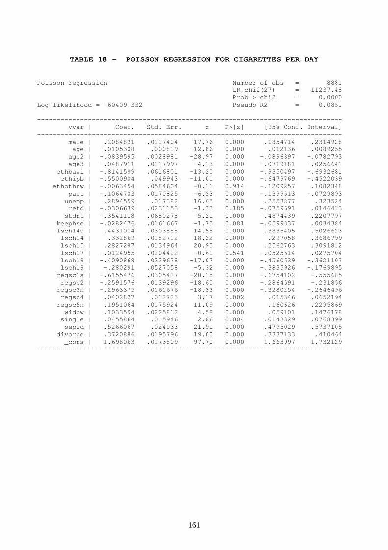
9.2 An application to cigarette smoking

61

Table 18 shows an example of the Poisson regression model. The dependent variable is

the number of cigarettes smoked per day by respondents to the HALS. Respondents are

asked to report the actual number of cigarettes and the variable can be interpreted as a

count. The model estimates the number of cigarettes smoked as a function of the usual

list of explanatory variables. Table 18 reports the coefficients, standard errors and

implied z-ratios for each of the variables. Recall that the coefficients relate to the

intensity of the process, which is a non-linear function of the x’s. So the β’s are not

measured in the original units of the count data and inferences about the impact of a

particular variable on the actual number of counts have to be made by re-transforming

the coefficient estimates. However, we can use the coefficients to analyse the

qualitative impacts of the variables. So, for example, the results show a strong socio-

economic gradient in the number of cigarettes smoked, with those in professional and

managerial occupations having negative coefficients and the variables for semi-skilled

and unskilled occupations having positive coefficients.

INSERT TABLE 18

Inferences about quantitative effects can be made by calculating the marginal effect for

a continuous explanatory variable, say xk , which is given by the formula,

∂E(y|x)/∂xk = βkexp(xβ) (7)

while the formula for the average effect of a binary variable is,

E(y| xk =1) - E(y| xk =0) = exp(xβ| xk =1) - exp(xβ| xk =0) (8)

As with binary choice models, it is clear that these marginal and average effects depend

on the values of the other explanatory variables. Again, standard practice is to evaluate

these at the mean of the other x’s but estimates can be calculated for every individual in

the sample. Average effects for the discrete regressors and marginal effects for the

continuous regressors are given in Table 19, along with the mean value of each

regressor.

62

INSERT TABLE 19

The results in Tables 18 and 19 are estimated by maximum likelihood, assuming that

the Poisson distribution is appropriate for the data on the number of cigarettes smoked.

In fact, this is unlikely to be valid. In particular, there is a very high proportion of zeros

in the observed data. Around 70% of individuals were not current smokers at the time

of the survey. Among other things, this means that the conditional mean of the data

does not equal the conditional variance and leads us to look for specifications that allow

for over-dispersion and what are known as “excess zeros”. In other words, the data

exhibit a higher frequency of zero observations than would be predicted by the simple

Poisson model.

One possible explanation for over-dispersion and excess zeros is additional individual

heterogeneity beyond differences that can be summarised by the observed explanatory

variables. Mullahy (1997) emphasises that the presence of excess zeros in count data

can be seen as a strict implication of unobservable heterogeneity. Up to now individual

differences only enter the model through differences in the x variables. If there are

additional unobservable differences across individuals, these could be added as an extra

unobservable variable or error term. The effect of adding this further heterogeneity is to

spread out the distribution of the count variable, meaning that more observations are

shifted to the tails of the distribution so that we would expect to observe more zero

values and more high values than would be predicted by the simple Poisson model.

The most commonly applied model that allows for additional unobservable

heterogeneity is the negative binomial or negbin model which allows for over-

dispersion by assuming that the individual error term comes from a particular

probability distribution (the gamma distribution). By assuming the gamma

distribution it is possible to write down a new probability function for y and hence to

estimate the model by maximum likelihood estimation. The negbin model is more

flexible and relaxes the equi-dispersion property of the Poisson model. Two special

cases of the negbin model are typically estimated in practice: one in which the variance

63

of y is proportional to the mean of y and the other in which the variance is a quadratic

function of the mean. An attractive feature of the negbin model is that it nests the

Poisson model as a special case and this can be tested using a conventional t-test on the

coefficient that reflects over-dispersion. The negbin model has been applied

extensively in studies of health care utilisation (see Jones (2000) for a review of this

literature).

Table 20 shows estimates of a negbin model for the number of cigarettes smoked. The

conditional mean function for the negbin model is still an exponential function of the

explanatory variables and the coefficients should be interpreted in just the same way as

the Poisson model. The additional parameter, α, estimates the degree of over-dispersion

in the data. By default Stata estimates the negbin2 version of the model in which the

variance is a quadratic function of the mean. This parameter is large (8.257) and highly

significant. In this example there is strong evidence to reject the Poisson specification

as a special case of the negbin. The qualitative results for the negbin model are broadly

comparable with those of the Poisson model, so for example, we again see a socio-

economic gradient in the level of smoking, and there are some small changes in the

magnitude of the coefficients and substantial changes in the standard errors and t-ratios.

INSERT TABLE 20

Recall that our dependent variable is heavily influenced by a large proportion of zero

observations - around 70% of the sample. It is likely that much of the distinction

between smokers and non-smokers is now being picked up by the estimate of over-

dispersion. However, like the Poisson model, the negbin model assumes that there is a

single process underlying all of the observed values of the dependent variable, whether

y equals 0 or is greater than 0. Other recent developments of count data regression have

been based on the idea that there is something special about the zero observations and

that they are not just a reflection of over-dispersion. This makes a qualitative

distinction between participants and non-participants; for example, between those who

use health care and those who do not, or between smokers and non-smokers. One

64

example of this kind of approach are so-called zero-inflated models. These are an

example of mixture models. They take a standard count data model such as the Poisson

or negative binomial and add extra weight to the probability of observing a zero value.

This probability can be interpreted as a splitting mechanism which divides individuals

into non-users, with a probability q, and potential users with probability 1-q. The

probability q may be a function of a set of explanatory variables. So, in the zero-

inflated model the probability of observing zero is made up of the probability of

someone being a non-user plus the probability that they are a potential user, multiplied

by the probability of observing a zero under the standard count data model.

Tables 21 and 22 show estimates of the zero-inflated negative binomial regression for

the number of cigarettes smoked (again the estimated model is a negbin2 specification).

The first set of results assumes the splitting mechanism is just a constant. The second

allows explanatory variables to influence the splitting mechanism. These show

evidence of a split between non-smokers and potential smokers and also that this split is

influenced by observable explanatory variables – many of the variables that appear in

the splitting equation, labelled inflate in Table 22, are statistically significant. Notice

also that there are now substantial differences in both the sign and the size of the

regression coefficients for the negbin regression model compared to the specification

that did not allow for zero inflation. For example, the negbin results in Table 22 no

longer show such a clear socio-economic gradient in the level of smoking. This

suggests that the earlier results were largely driven by the distinction between smokers

and non-smokers, and that effectively the count data regressions were acting like binary

choice models, explaining whether someone smokes rather than how much they smoke.

INSERT TABLE 21

INSERT TABLE 22

The zero-inflated specification separates out the binary choice of whether to smoke or

not from the number of cigarettes smoked given that someone is a smoker. Another

way of dealing with this distinction between participants and non-participants is to use a

so-called hurdle or two-part specification. This assumes that the participation decision

65

and the positive values of the count data are generated by two separate probability

functions. In some applications, the participation decision is modelled using a standard

binary choice model such as the logit or probit. In others, a count data specification

such as the Poisson or negbin model is used, with a dependent variable that can take

values of either 0 or 1. Then a standard count data regression is applied to the sub-

sample of participants, allowing for the fact that the count data is truncated at zero.

When faced with count data that exhibit over-dispersion and a large proportion of zero

observations, analysts are faced with a choice of two types of specification: those that

emphasise the role of unobservable heterogeneity, such as the negbin model; and those

that emphasise the special role of zero observations, such as zero-inflated or hurdle

models. Applications of zero-inflated or hurdle models often make the probability of

participation a function of explanatory variables, as interest lies in the type of factors

that distinguish users and non-users of health care, or smokers and non-smokers.

Applications of the negbin model often treat over-dispersion as a fixed parameter and

do not allow it to be a function of the explanatory variables. This may bias the

comparison in favour of zero inflated and hurdle models. The negbin model also relies

on a specific functional form for the unobservable heterogeneity. Recent work in the

health economics literature has advocated a more robust and flexible approach, which

treats unobservable heterogeneity in a non-parametric way: the finite mixture approach

to model health care utilisation. In this approach, the unobservable heterogeneity is

treated as a discrete random variable where each category of the variable represents an

unobservable “type” of individual. So, for example, with a 2-point mixture there would

be two types, such as “healthy” and “ill” individuals. These two values are known as

points of support.

In the finite mixture approach, the probability of an individual belonging to one of these

types is estimated along with the other parameters of the model. Deb and Trivedi

(1997) apply finite mixture models with two and three points of support for data on the

demand for medical care among individuals aged 66 and over in the 1987 US medical

care expenditure survey. Demand is measured by six different indicators of annual

health care utilisation and the finite mixture model is compared to hurdle and zero-

66

inflated specifications. The negbin models with two points of support are preferred on

the basis of various statistical criteria. Deb and Trivedi interpret the points of support as

two latent populations of “healthy” and “ill” individuals reflecting unobservable

differences in frailty across the population.

67

Appendix: Stata code for count data regression

The count data regression models are applied to ‘fagday’, the number of cigarettes

smoked per day:

replace yvar=fagday Poisson regression

The starting point is the Poisson regression model. Predictions are saved for both the

fitted values of the nonlinear regression function, exp(xβ) and for the linear index, xβ:

poisson yvar $xvars * predict exp(xb) predict fitted, n predict yf, xb

Partial effects of the regressors on the actual number of cigarettes smoked need to take

account of the nonlinearity of the regression function, exp(xβ). Here we compute the

average effect for ‘unemp’:

scalar bunemp=_b[unemp] gen ae_unemp=0 replace ae_unemp=exp(yf+bunemp)-exp(yf) if unemp==0 replace ae_unemp=exp(yf)-exp(yf-bunemp) if unemp==1 summ ae_unemp hist ae_unemp

One way of assessing the performance of the model is to tablulate the actual and fitted

values of y against each other. To do this the fitted values are rounded to the nearest

integer value: replace fitted=round(fitted) tab fitted yvar

The RESET test for the Poisson model follows the usual format: gen yf2=yf^2 quietly poisson yvar $xvars yf2 test yf2

68

To exploit the pseudo maximum likelihood (PML) property of Poisson regression the

model can be estimated using robust standard errors:

poisson yvar $xvars, robust The negbin model

To relax the equidispersion property that is implicit in the Poisson model we can run a

negative binomial (negbin) regression and recalculate partial effects and the fitted

values:

nbreg yvar $xvars predict yf, xb predict fitted *PARTIAL EFFECTS scalar bunemp=_b[unemp] gen ae_unemp=0 replace ae_unemp=exp(yf+bunemp)-exp(yf) if unemp==0 replace ae_unemp=exp(yf)-exp(yf-bunemp) if unemp==1 summ ae_unemp hist ae_unemp scalar drop bunemp drop ae_unemp replace fitted=round(fitted) tab fitted yvar

By default Stata estimates the negbin2 version of the model in which the variance is a

quadratic function of the mean. The alternative negbin1 specification, in which it is a

linear function, can be obtained by using the sub-command dispersion(constant). A

more general specification allows the overdispersion to be a function of the x variables

as well as the conditional mean:

gnbreg yvar $xvars, lna($xvars) predict fitted replace fitted=round(fitted) tab fitted yvar Zero-inflated models

69

The Poisson, negbin and generalised negbin models all assume the same mean function,

exp(xβ). This may not be flexible enough to model a dependent variable with excess

zeros. One alternative is the zero-inflated model that adds an additional probability of

observing a zero. The simplest form of the zero-inflated Poisson (ZIP) model treats this

probability as a constant: zip yvar $xvars, inflate(_cons) vuong predict fitted predict yf replace fitted=round(fitted) tab fitted yvar Computation of the partial effects needs to take account of the change in the mean

function in the ZIP model:

scalar bunemp=_b[unemp] scalar qi=_b[inflate:_cons] scalar qi=exp(qi)/(1+exp(qi)) scalar list qi gen ae_unemp=0 replace ae_unemp=(1-qi)*(exp(yf+bunemp)-exp(yf)) if unemp==0 replace ae_unemp=(1-qi)*(exp(yf)-exp(yf-bunemp)) if unemp==1 summ ae_unemp hist ae_unemp A more flexible version of the ZIP allows the zero-inflation probability q to depend on

the regressors. This model can be difficult to estimate in practice and estimates may not

converge: zip yvar $xvars, inflate($xvars _cons) predict pi, p predict fitted replace fitted=round(fitted) tab fitted yvar

Similar syntax applies for the zero-inflated negbin model. The option to report the

‘Vuong’ statistic allows the ZIP and standard models, which are non-nested, to be

compared:

zinb yvar $xvars, inflate(_cons) vuong predict fitted replace fitted=round(fitted) tab fitted yvar zinb yvar $xvars, inflate($xvars|_cons) vuong

70

predict fitted replace fitted=round(fitted) tab fitted yvar Hurdle models

A common alternative to the zero-inflated model is the hurdle model. The first stage of

the hurdle model is often estimated as a standard logit model: replace yvar1=regfag logit yvar1 $xvars Followed by truncated regressions (either Poisson or negbin) at the second stage:

ztp yvar $xvars ztnb yvar $xvars

71

Chapter 10 Duration Analysis

10.1 Duration data

The previous section discussed count data models, where the dependent variable is the

number of events occurring over a period of time, for example the number of GP visits

over the previous month. A closely related topic is duration analysis. Here, the focus is

on the time elapsed before an event occurs, rather than on the number of events. So, for

example, duration could measure the number of years that someone lives from birth; or

it could measure a patient’s length of stay after admission to hospital; or it could

measure the number of years that someone smoked cigarettes.

Once again, the HALS can be used to provide a useful illustration of the application of

duration analysis. Forster and Jones (2001) used duration analysis to explore two

aspects of smoking: the decisions to start and to quit. Here, there are two measures of

duration: the age at which somebody starts smoking cigarettes and the number of years

that they smoke once they have started. By analysing these two variables we can learn

about the impact of individual characteristics on the probability of starting and the

probability of quitting smoking. Recall that the original HALS data were collected in

1984-85. The survey included information that allows individuals to be divided into

those who were regular smokers at the time of the survey, those who had been regular

smokers but had quit by the time of the survey and those who had never smoked prior to

the survey.

The current and ex-smokers in the survey were asked how old they were when they

started to smoke cigarettes. This is self-reported retrospective data and so may be prone

to problems of measurement error, such as recall bias. Recall bias occurs when

respondents have difficulty recalling events from their past, it includes phenomena such

as ‘telescoping’ of events and ‘heaping’ of observations at round-numbers.

For those who had started smoking at some time prior to the survey, we observe the

72

actual value of duration and their age when they started smoking. For those individuals

who had not smoked prior to the survey, there is a problem of censoring. In other

words, all we know is that they had not started smoking prior to the date of the

interview. It is possible that some of these individuals will go on to start smoking at a

later age. All we know is that their age of starting is at least as great as their age at the

time of the survey, and, for this reason we refer to them as right censored observations.

So for these individuals, we can use the probability that their true duration is greater

than the censored value - in this case, their age at the time of the HALS. Standard

models of duration data are built on the assumption that eventually everyone will “fail”.

In this application, this would mean that eventually all individuals will start smoking.

This is unlikely to be plausible in the case of smoking and, as we shall see below, it is

possible to relax the specification to allow some individuals to remain non-smokers.

For those who become smokers the second measure of duration is the number of years

that they smoke. This helps us to analyse the probability of quitting. This new variable

can be defined by taking the individuals’ ages at the time of the interview and

subtracting the ages that they started smoking. For those individuals who had already

quit smoking prior to the survey, the number of years since they quit should also be

subtracted. Once again, there is a problem of right censoring. For those individuals

who had quit prior to the survey, we observe a complete spell. For those individuals

who were still current smokers at the time of the survey, all we know is the age that they

started and the fact that they are still smoking in 1984-85. For these individuals we can

only estimate the probability that they have survived (as smokers) for at least that many

years, given their characteristics.

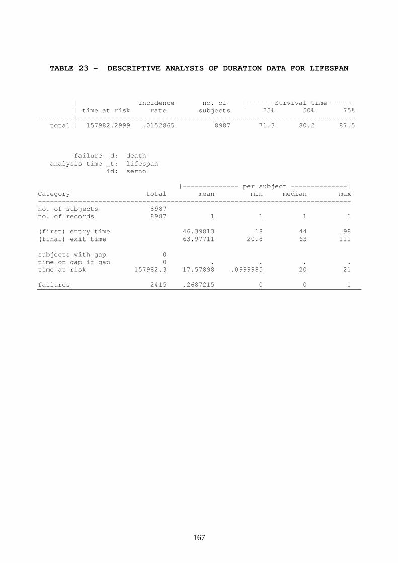
The HALS data provide us with a third measure of duration. The survey respondents

were linked with the NHS Central Register of Deaths, which provides information on

survival rates. For respondents who had died by June 2005 (in the latest release of the

deaths data), the survey provides information on their age and cause of death taken from

death certificates. This third measure of duration is an individual’s lifespan in years,

with the origin defined as an individual’s birth and the duration measured up to their age

at death. Once again, there is a problem of right censoring. For those individuals who

73

died between the collection of the HALS data in 1984 and the collection of the deaths

data in 2005, we observe a complete spell. The majority of the original HALS

respondents were still alive in 2005, and these represent right censored observations.

But the deaths data raise a further issue, the problem of left truncation. The natural

origin for the measure of lifespan is an individual’s birth. However, the HALS was

designed as a representative random sample of the living population in 1984. To be

included in the survey, an individual must have survived at least to their age at the time

of HALS. An individual who was born and died prior to HALS is a form of missing

data. For each age group the probability of surviving to the time of the survey may

vary systematically across different types of individuals. This creates a source of bias -

the problem of left truncation. To deal with this, the duration models need to be

adapted to incorporate the probability that an individual survives at least to their age at

the time of HALS.

10.2 Survival analysis

Analysis of models of survival or duration revolves around the notion of a hazard

function h(t). This measures the probability that someone fails at time t, given that they

have survived up to that point. It can be written as,

h(t) = f(t)/S(t) (9)

where the two components on the right-hand side are the probability density function

(f(t)), the probability of failing at time t, and the survival function (S(t)), which is the

probability that someone survives to at least time t. In estimating duration models, the

density function is used for uncensored observations, where we observe their actual

time of failure, and the survival function is used for censored observations where we

only know they have survived at least to time t.

Parametric models of duration assume particular functional forms for f(t) and S(t) and

therefore for the hazard function h(t). A common example is the Weibull model. The

74

hazard function for the Weibull model takes the form,

h(t) = hptp-1. exp(xβ) (10)

where h and p are parameters to be estimated. This develops the kind of regression

model we have seen in previous chapters in that it is not just a function of the

explanatory variables x but also of duration itself (t). The first term on the right hand

side of equation (10), hptp-1, is known as the base-line hazard. This defines the

relationship between the hazard of failure and the duration (t). The shape of the base-

line hazard allows us to estimate how the hazard function changes with time. In the

Weibull model the parameter p is known as the shape parameter. The hazard function is

increasing for p > 1, showing increasing duration dependence, while it is decreasing for

p < 1, showing decreasing duration dependence. Duration dependence may be of

interest in itself. For example, we may want to learn whether the probability of someone

receiving a job offer increases or decreases the longer they have been unemployed. In

addition to learning about duration dependence, duration analysis allows us to estimate

the impact of individual characteristics (the x’s) on the probability of failure. These are

captured by the second term in equation (10), exp(xβ), which leads to proportional

shifts in the base-line hazard for individuals with different characteristics (x).

Parametric models rely on fully specifying the base-line hazard function. The chosen

functional form may not be valid and it is particularly vulnerable to problems caused by

unobservable heterogeneity across individuals. A more flexible approach is to use a

semi-parametric model. The best known example is the Cox proportional hazard

model. This leaves the baseline hazard unspecified, treated as an unknown function of

time. Because the method does not require specification of the baseline hazard, it is

more robust than parametric approaches. In order to implement the method, the

duration data are converted into a rank ordering of individuals according to their level

of duration, t. Because this throws away information on the actual value of t, the

method is less efficient than a parametric approach.

Analysis of the age of starting smoking is more complicated. As mentioned earlier,

75

standard duration models assume that eventually everyone fails - in this case everyone

would eventually start smoking. This seems to be an implausible assumption, and

models based on the assumption do not do a good job of fitting the observed data. An

alternative is to use a so-called split population model. This augments the standard

duration analysis by adding a splitting mechanism analogous to the zero- inflated

models of count data. So, for example, a probit specification could be added to model

the probability that somebody will eventually start smoking. When this splitting

mechanism is added to the duration model, it does a far better job of explaining the

observed data on age of starting than models that omit a splitting mechanism (see

Forster and Jones, 2001).

As with count data, dealing with unobservable heterogeneity is a particular

preoccupation in the literature on duration models. The existence of unobservable

heterogeneity will bias estimates of duration dependence. For example, consider the

case where there are two types of people: “frail” individuals who have a high (but

constant) hazard rate and “strong” individuals who have a low (but constant) hazard

rate. The two groups may be equally mixed in the population to begin with, but over

time the frailer individuals will tend to die first, leading to an unequal mix. As time

passes the proportion of frail individuals will decrease and the overall hazard will

decrease. If it is not possible to control for the heterogeneity between the two types of

individual, this will give the appearance of decreasing duration dependence.

Unobservable heterogeneity can be dealt with by adding an extra error term to the

model. Like count data models, this can be dealt with parametrically by assuming a

particular functional form for the distribution of the error term. Alternatively, a non-

parametric approach can be adopted, using the finite mixture model. This assumes that

the unobservable error term has a discrete distribution characterised by a set of mass

points, where the value of these mass points and the probabilities attached to them are

estimated as part of maximum likelihood estimation.

10.3 An application to the HALS deaths data

76

The measure of survival time used in this application is each individual’s lifespan. The

entry date is the individual’s date of birth and the exit date is June 2005, the time of the

latest release of the HALS deaths data. Lifespan is left truncated, as the duration is only

observed for those individuals who survived up to the HALS1 interview data, so the left

truncation variable is age at HALS1. Those individuals who are still alive at June 2005

have incomplete spells and are treated as censored observations. Table 23 reports

descriptive evidence from the ‘stsum’ and ‘stdes’ commands for survival data. These

show that the first quartile of survival time is 71 years, the median is 80 and the upper

quartile is 87. They confim that the data only contains one record per subject and that

the average time of entry (age at HALS1) is 45 and the average time of exit is 64. The

latter includes all of the incomplete spells – those still alive in June 2005. There are

2415 cases who had died by June 2005.

INSERT TABLE 23

Before moving to the survival regressions, Figures 2-4 show the nonparametric

estimates of the survival and hazard functions. The Kaplan-Meier estimate of the

survival function, in Figure 2, remains fairly flat (with a high probability of survival)

until the mid-60s age range. It then drops off rapidly, approaching zero as the age range

reaches the late 90s. This pattern is reflected in the shape of the Kaplan-Meier estimate

of the hazard function (Figure 3) and Nelson-Aalen estimate of the cumulative hazard

function (Figure 4). The hazard is smooth and monotonically increasing. It remains flat

until around age 60 and then increases quite dramatically as the risk of death rises with

age. The dip in the hazard function at the extreme right of the age range is an artefact of

the sparsity of data for the very elderly in HALS.

INSERT FIGURE 2

INSERT FIGURE 3

INSERT FIGURE 4

We move now to the survival regressions, that model the hazard as a function of a

reduced set of our usual set of covariates. Table 24 presents the Cox proportional hazard

77

model. The coefficients are reported in the form of exp(β) and should be intepreted as

upwards (>1) or downwards (<1) parallel shifts in the baseline hazard function. The

results show some evidence of a gradient by education: those who left school later

always have a lower probability (hazard) of death. The same applies to the social class

gradient where the higher social classes have a lower hazard.

INSERT TABLE 24

The model in Table 25 uses a parametric baseline hazard – in this case the Weibull

model. Like Table 24 the results are presented in proportional hazard format and can be

compared directly to those for the Cox model (which leaves the baseline hazard

unspecified). It is clear that the estimates are very similar for both models. The estimate

of the duration dependence parameter, p, is 7.382 showing strong positive duration

dependence, as we would expect from the nonparametric plot of the hazard function.

This is reflected in the plot of the fitted survival (Figure 5), hazard (Figure 6) and

cumulative hazard (Figure 7) functions for the Weibull model, which are comparable to

the nonparametric estimates.

INSERT TABLE 25

INSERT FIGURE 5

INSERT FIGURE 6

INSERT FIGURE 7

Finally Table 26 presents estimates for the same Weibull model presented in accelerated

time to failure format. This reformulation of the model can be interpreted as a

regression of the x variables on the logarithm of lifespan. So the estimated coefficients

should be interpreted in terms of changes in the logarithm of lifespan (ln(T)). A positive

sign means increased lifespan and a negative sign reduced lifespan for individuals with

a particular characteristic. So while Table 25 presents results for exp(β), the coefficients

in Table 26 give -lnexp(β)/p.

78

INSERT TABLE 26

79

Appendix: Stata code for duration analysis

The measure of survival time used in the application is each individual’s lifespan. The

entry date is the individual’s date of birth and the exit date is June 2005, the time of the

latest release of the deaths data. Lifespan is left truncated, as the duration is only

observed for those individuals who survived up to the HALS1 interview data, so the left

truncation variable is age at HALS1. Those individuals who are still alive at June 2005

have incomplete spells and are treated as censored observations. These features of the

data are encoded in the ‘stset’ command: stset lifespan, failure(death) id(serno) time0(age) Once this has been specified the duration variable ‘lifespan’ can be summarized:

stsum stdes Before proceeding to the estimation of survival regressions it is important to explore

nonparametric plots of the survival and hazard functions. Nelson-Aalen and Kaplan-

Meier estimates can be computed and the plots saved to files for subsequent use:

sts graph, na title("NA ls") saving(lsNA, replace) sts graph, hazard title("KM hazard ls") saving(lsHkm, replace) sts graph, title("KM Survival ls") saving(lsKMsurv, replace)

The first regression model to be estimated is the Cox proportional hazard model, which

leaves the baseline hazard unspecified. This uses a reduced set of regressors that capture

ethnic group, education and social class, defined by the global ‘$xls’: stcox $xls The parametric Weibull model can be estimated in comparable proportional hazard

format:

streg $xls, d(weibull) nolog

80

Or it can be estimated using the accelerated time to failure version:

streg $xls, d(weibull) nolog time

This is followed up by commands to plot and save the fitted survival, cumulative hazard

and hazard functions:

stcurve, survival title("Ls survival") saving(lssurv, replace) stcurve, cumh title("Ls cumh") saving(lscumh, replace) stcurve, hazard title("Ls hazard") saving(lshaz, replace)

81

Chapter 11 Panel Data Models

11.1 Linear models

With the exception of duration analysis, all of the models described so far have been

applied to a single cross-section survey, where each individual is observed only once.

With panel data a longitudinal element is added to the data and there are repeated

measurements for each individual observation. Panel data are closely related to

multilevel data where observations are grouped within organisations or geographic

areas: for example, a survey of patients, within specialties, within hospitals. Multilevel

models have a similar structure to models for panel data and are not discussed here (see

the suggestions for further reading).

Recall that the original HALS cross-section study was repeated seven years later in

1991-92. Rather than drawing a new random sample of individuals, the original HALS

respondents were revisited and asked to complete the same face-to-face interview, nurse

visit and postal questionnaire as in the original study. So, for each variable in the

survey, and for each individual respondent we observe two values. With only two

waves, HALS is an example of a so-called “short” panel where the number of

individuals, n, is far greater than the number of waves, T. Longitudinal data add a new

dimension to the analysis and allow researchers to explore the dynamics of individual

behaviour. They also provide more scope for dealing with individual heterogeneity.

Consider a standard linear regression model in which there are repeated measurements

(t = 1,....,T) for a sample of n individuals (i=1,....,n),

yit = xitβ + αi + εit (11)

Here the dependent variable y is observed for individual, i, in each of the waves, t.

Similarly, the explanatory variables x are observed at each wave. Some of these

82

variables will be time varying (for example, an individual’s income at different points

of time). Others may be fixed or time invariant (such as an individual’s gender or

ethnic background). In practice, with the kind of short panels discussed here, the

regressors may also include a set of dummy variables for each wave of the panel (with

one wave omitted for the reference period) in order to capture time effects. The error

term of the regression equation (11) has been split into two components (this is known

as an error components model). The first term, αi is an individual-specific

unobservable effect - the unobserved characteristics of the individual i that remain

constant over time. The second term, εit, is a random error term representing

idiosyncratic shocks that vary over time. Typically, it is assumed that αi and εit are

uncorrelated with each other. The critical issue for the estimation of panel data models

is whether the individual effects αi are correlated with the observed regressors x.

Failure to account for correlation between αi and x in estimating the panel data

regression model leads to inconsistent estimates of the slope coefficients, β.

The presence of a common individual effect means that the values of the dependent

variable for each individual will tend to cluster together. This clustering can be allowed

for using the generalised least squares estimator (GLS) which allows for the fact that

an error term for a particular individual will be correlated over the waves of the panel.

However, use of the GLS estimator assumes that the individual effect is uncorrelated

with the explanatory variables x. This problem can be dealt with by using deviations to

sweep the unobservable individual effect out of the equation. One way of doing this is

to adopt a fixed effects approach and take mean deviations, measuring each variable as

the deviation from within-individual mean of the variables. Alternatively the variables

can be measured as first differences (by subtracting the value in period t-1 from the

value in period t). Because the individual effect is assumed to be constant over time,

taking deviations eliminates α from the equation. Applying the standard least squares

estimator to the transformed variables gives the covariance or within-groups estimator

of β, which is consistent even when the individual effect is correlated with the

explanatory variables. However, for this estimator to work in practice, there must be

sufficient within-individual variability in the dependent variable and the explanatory

variables. The estimator will tend not to work well in a short panel (where T is small)

83

and where there is not much variation within groups. These problems go away when

the group size is large, in other words when T is large. In that case the GLS or random

effects estimator can be shown to be equivalent to the within-groups or fixed effects

estimator.

The random effects and fixed effects estimators for the linear panel data model are

illustrated using data on the number of cigarettes smoked per day for the sub-sample of

smokers in the HALS data. Table 27 shows the random effects GLS regression and

Table 28 shows the fixed effects within-groups regression. The models are estimated

using the two waves of the HALS data. As some individuals who took part in the first

survey did not respond to, or could not be traced, for the second survey, the models are

estimated on the unbalanced panel, using all available observations on the dependent

variable. This means that more data are included for individuals at wave 1 than for

wave 2.

INSERT TABLE 27

In the GLS model, the error components specification means that the overall variance of

the error term can be decomposed into two components, σ2α associated with the

individual effect and σ2ε associated with the idiosyncratic error term. Table 27 gives

estimates of σα (sigma_u) and σε (sigma_e) and also reports the value of ρ, the intra-

group correlation coefficient, which has a value of 0.585. This shows the fraction of the

overall variance of the error term that can be attributed to the individual effect. The

coefficients of the regression function can be interpreted in the usual way. They show,

for example, that individuals with more years of schooling smoke fewer cigarettes and

those with fewer years of formal schooling smoke more.

INSERT TABLE 28

As it only has two waves, the HALS data are not well-suited to the fixed effects

estimator, particularly as the two waves are seven years apart. In applying the within-

groups estimator, any time invariant variables, such as the individual’s gender or ethnic

84

group are eliminated from the regression. The remaining variables are measured as

deviations from the within-individual mean. Table 28 is included only for comparison

with the random effects estimates. The fact that HALS only has two waves means that

the within-groups estimator performs very poorly. The method would come into its own

with a longer panel, providing more information on each individual’s behaviour as it

evolves over time.

11.2 Binary choices

The discussion so far has concentrated on a simple linear panel data regression model in

which the dependent variable can take a continuous range of values. In practice,

analysts using health surveys are more likely to be confronted with qualitative or

categorical dependent variables, these make estimation of panel data models more

complex. The linear specification is attractive because taking differences or mean

deviations allows the individual effect to be swept from the equation. But this is no

longer possible for a non-linear regression model as typically used for qualitative and

categorical variables. To illustrate, consider a binary choice model,

E(y |xitβ, αi) = P(yi=1|xitβ, αi) = F(xitβ + αi) (12)

Taking differences or mean deviations of the non-linear function F(.) will not eliminate

the individual effect. This is a problem if the individual effects are expected to be

correlated with the explanatory variables.

If an analyst is willing to assume that the effects and the explanatory variables are

uncorrelated, then the clustering of the dependent variable can be dealt with using a

random effects specification. For example, the random effects probit model assumes

that both components of the error term are normally distributed and that both are

independent of xit. By assuming a specific distribution for the individual effect it is

possible to write down a sample log likelihood function that allows for the correlation in

the error term within individuals. This expression can be estimated using standard

85

software, such as Stata.

Let us return to the example of the binary measure of self-assessed health, where y

equals 1 if an individual reports “excellent” or “good” health and equals 0 if an

individual reports “fair” or “poor” health. Now we can make use of the longitudinal

element of HALS and use information from both waves of the survey. The first set of

estimates, presented in Table 29, are for a pooled probit specification. This simply

takes the standard probit estimator and ignores the fact that we are dealing with repeated

observations. It pools all of the observations together, not allowing for the fact that

individuals are measured twice. This means that the model is estimated on the basis of

a wrongly specified likelihood function. However, it can be shown that the estimator

does give consistent estimates of the population averaged coefficients, even though it

ignores the structure of the error term. However robust standard errors should be used

that allow for the clustering of observations within individuals. Compare these estimates

with the cross-section results for the probit model in Chapter 3. Now we have a larger

sample because we are using information from wave 2 as well as wave 1. Again, the

coefficients should be interpreted as qualitative effects and quantitative inferences

should be made on the basis of average or marginal effects. Once more, we can see

clear gradients in self-assessed health by education and by occupational socio-economic

group.

INSERT TABLE 29

Table 30 shows the random effects probit model. The Table includes an estimate of ρ,

the intra-group correlation coefficient. This suggests that the individual effect accounts

for around half (0.532) of the random variation

INSERT TABLE 30

Recall that the random effects probit model embodies two important assumptions: that

86

the individual effect has a normal distribution and that it is uncorrelated with the

explanatory variables. The first assumption can be relaxed by using a semiparametric

approach. For example Deb (2001) develops a finite mixture random effects probit

model, using the same sort of methods that were described in the chapters on count data

and duration models.

The second assumption - that the individual effects are uncorrelated with the

explanatory variables - can be dealt with in two ways. The first is to adopt a fixed

effects specification, treating the individual effects as parameters to be estimated, or at

least eliminated from the model. The second is to use a correlated random effects

specification. It has already been stressed that, for most non-linear models, the

convenient device for taking mean deviations or first differences is no longer feasible.

This is certainly the case for the panel data probit model. However, the logit model is

an exception to this rule. Because of the special features of the logistic function, it is

possible to re-formulate the model in a way that eliminates the individual effect, α.

This is known as the conditional logit model. For example when there are only two

waves in the panel (T=2), by restricting attention to those individuals who change status

during the course of the panel, it is possible to estimate the standard logit model using

first differences in the explanatory variables, rather than the levels of the variables. This

means that the standard logit model can be applied to differenced data and the

individual effect is swept out in the process. Like the fixed effects estimator for linear

models, this approach will work well only if there is sufficient within-individual

variation in the variables.

Another approach to dealing with individual random effects that are correlated with the

explanatory variables is to specify this relationship directly. For example, in dealing

with the random effects probit model, Chamberlain suggested specifying this

relationship as a linear regression of the value of the explanatory variables in all of the

waves of the panel. A convenient special case of this approach, which just includes

within-individual means of the regressors, had been suggested earlier by Mundlak. This

function is then substituted back into the original equation and, as long as there is

sufficient within individual variation, it allows separate estimates of the βs and of the

87

correlation between the x’s and the individual effect to be disentangled (see the

Technical Appendix and Jones, 2000, for details of this method). In this sense, this

method has a strong parallel with the within-group estimator.

11.3 Simulation-based estimation

The random effects probit model only involves a univariate integral. More complex

models, for example where the error term is assumed to follow an autoregressive

process lead to sample log-likelihood functions that involve higher order integrals.

Monte Carlo simulation techniques can be used to deal with the computational

intractability of nonlinear models, such as the panel probit model and the multinomial

probit. Popular methods of simulation-based inference include classical Maximum

Simulated Likelihood (MSL) estimation, and Bayesian Markov Chain Monte Carlo

(MCMC) estimation.

Classical methods

We can use Monte Carlo (MC) simulation to approximate integrals that are numerically

intractable. MC approaches use pseudo-random selection of evaluation points and

computational cost rises less rapidly than with quadrature. The principle behind

simulation-based estimation is to replace a population value by a sample analogue. This

means that we can use laws of large numbers and central limit theorems to derive the

statistical properties of the estimators.

The idea behind Maximum Simulated Likelihood (MSL) is to replace the likelihood

function with a sample average over R random draws. Consistency and asymptotic

unbiasedness can be obtained by reducing the error in the simulated sample log-

likelihood to zero as R→∞ at a sufficient rate with n. A sufficient rate is R/√n→∞ as

n→∞ and this is sufficient for the usual MLE estimate of the covariance matrix to be

used without any correction.

88

Bayesian MCMC methods

In Bayesian analysis a prior density of the parameters of interest is updated with the

information contained in the sample. Given a specified sample likelihood the posterior

density of the parameters of interest is given by Bayes' theorem. The posterior density

reflects updated beliefs about the parameters. Given the posterior distribution, a 95%

credible interval can be constructed that contains the true parameter with probability

equal to 95%. Point estimates for the parameters can be computed using the posterior

mean.

Bayesian estimates can be difficult to compute. In order to overcome the difficulties in

obtaining the characteristics of the posterior density, Markov Chain Monte Carlo

(MCMC) methods are used. The methods provide a sample from the posterior

distribution. Posterior moments and credible intervals are obtained from this sample.

MCMC algorithms yield a sample from the posterior density by constructing a Markov

Chain which converges in distribution to the posterior density. In a Markov chain each

value is drawn conditionally on the previous iteration. After discarding the initial

iterations, the remaining values can be regarded as a sample from the posterior density.

MCMC algorithms are usually based on Gibbs sampling, sometimes complemented by

the Metropolis-Hastings (M-H) algorithm. These methods are outlined in the technical

appendix. The algorithms can be extended to deal with missing data using data

augmentation in which latent or missing data are regarded as parameters to be

estimated. Although data augmentation introduces many more parameters into the

model, the conditional densities usually belong to well-known families and there are

simple methods to sample from them. This makes the use of the Gibbs sampling

possible.

11.4 Attrition bias

Using panel data - such as the Health and Lifestyle Survey (HALS) and other panels

such as the British Household Panel Survey (BHPS) or European Community

89

Household Panel (ECHP) - to analyse longitudinal models of health creates a risk that

the results will be contaminated by bias associated with longitudinal non-response.

There are drop-outs from the panels at each wave and some of these may be related

directly to health: due to deaths, serious illness and people moving into institutional

care. In addition, other sources of non-response may be indirectly related to health, for

example divorce may increase the risk of non-response and also be associated with

poorer health than average. The long-term survivors who remain in the panel are likely

to be healthier on average compared to the sample at wave 1. The health of survivors

will tend to be higher than the population as a whole and their rate of decline in health

will tend to be lower. Also, the socioeconomic status of the survivors may not be

representative of the original population who were sampled at wave 1.

A broad definition of longitudinal non-response encompasses any observations that

“drop-out” from the original sample over the subsequent T waves. Non-response can

arise due to:

1. Demographic events such as death.

2. Movement out of scope of the survey such as institutionalization or emigration.

3. Refusal to respond at subsequent waves.

4. Absence of the person at the address.

5. Other types of non-contact.

The notion of attrition, commonly used in the survey methods literature, is often

restricted to points 3, 4 and 5. However our concern is with any longitudinal non-

response that leads to missing observations in the panel data regression analysis. In fact

it is points 1 and 2 – death and incapacity – that are likely to be most relevant as sources

of health-related non-response.

Testing

A simple variable addition test can be used to diagnose attrition bias in panel data

regressions. This involves adding a test variable, that reflects non-response, to the

original regression model and testing its significance. The test variables that can be used

are i) an indicator for whether the individual responds in the subsequent wave ii) an

indicator of whether the individual responds in all waves and, hence, is in the balanced

90

sample and iii) a count of the number of waves that are observed for the individual. The

t-ratios on the added variables provide three variants of the test for non-response bias.

The intuition behind these tests is that, if non-response is random, indicators of an

individual’s pattern of survey responses should not be associated with the outcome of

interest after controlling for the observed covariates. Additional evidence can be

provided by Hausman-type tests that compare estimates from the balanced, for whom

we have complete information at all waves, and unbalanced, for whom we have

incomplete information for some individuals, samples. In the absence of non-response

bias these estimates should be comparable, but non-response bias may affect the

unbalanced and balanced samples differently leading to a contrast between the

estimates. It should be noted that the variable addition tests and Hausman-type tests

may have low power to detect the problem of attrition bias; they rely on the sample of

observed outcomes and will not capture non-response associated with idiosyncratic

shocks that are not reflected in observed outcomes.

Estimation

One approach to dealing with attrition bias is to adopt the selection on unobservables

framework and use variants of the sample selection model described in Chapter 7. Here

we concentrate on an alternative approach, based on selection on observables. To allow

for non-response we can adopt an inverse probability weighted (IPW) estimator. This

approach is grounded in the notion of missing at random or ignorable non-response.

Using R as an indicator of response (R=1 if observed, 0 otherwise) and y and x as the

outcome and covariates of interest: missing completely at random (MCAR) is defined

by P(R=1|y,x)=P(R=1) and missing at random (MAR) is defined by

P(R=1|y,x)=P(R=1|x). The latter implies that, after conditioning on observed covariates,

the probability of non-response does not vary systematically with the outcome of

interest.

Fitzgerald et al. (1998) extend the notion of ignorable non-response by introducing the

concepts of selection on observables and selection on unobservables. This requires an

additional set of observables, z, that are available in the data but not included in the

regression model. Selection on observables is defined by Fitzgerald et al. by the

91

conditional independence condition P(R=1|y,x,z)=P(R=1|x,z). Selection on

unobservables occurs if this conditional independence assumption does not hold.

Selection on unobservables, also termed informative, non-random or non-ignorable non-

response, is familiar in the econometrics literature where the dominant approach to non-

response follows the sample selection model. This approach relies on the z being

“instruments” that are good predictors of non-response and that satisfy the exclusion

restriction P(y|x,z)=P(y|x). This is quite different from the selection on observables

approach that seeks z’s which are endogenous to y. Also it is worth mentioning that

linear fixed effects panel estimators are consistent, in the presence of selection on

unobservables, so long as the non-ignorable non-response is due to time invariant

unobservables.

The validity of the selection on observables approach hinges on whether the conditional

independence assumption holds and non-response can be treated as ignorable, once z is

controlled for. If the condition does hold, consistent estimates can be obtained by

weighting the observed data by the inverse of the probability of response, conditional on

the observed covariates. This gives more weight to individuals who have a high

probability of non-response, as they are under-represented in the observed sample.

Fitzgerald et al. (1998) make it clear that this approach will be applicable when interest

centres on a structural model for P(y|x) and that the z’s are deliberately excluded from

the model, even though they are endogenous to the outcome of interest. They suggest

lagged dependent variables as an obvious candidate for z. Of course, this approach will

break-down if an individual suffers an unobserved health shock, that occurs after their

previous interview, that leads them to drop out of the survey and that is not captured by

conditioning on lagged measures. In this case non-response would remain non-ignorable

even after conditioning on z.

It is possible to test the validity of the selection on observables approach. The first step

is to test whether the z’s do predict non-response; this is done by testing their

significance in the probit models for non-response at each wave of the panel. The

second is to do Hausman-type tests to compare the coefficients from the weighted and

unweighted estimates. Finally an inversion test can be used: conditioning on patterns of

92

response by splitting the sample into those in the balanced panel and the drop-outs and

then comparing models for the dependent variable in the initial wave estimated on the

sub-samples.

93

Appendix: Stata code for panel data models

To analyse panel data Stata needs to be given the individual identifier (i) and the time

identifier (t) and the data has to be sorted by these variables. In the HALS these are

given by the variables ‘serno’ and ‘wave’: iis serno tis wave sort serno wave

It is useful to create indicators of whether observations are in the balanced and in the

unbalanced estimation samples and a variable that records the number of waves for each

observation (Ti). This is done by running a regression model for fagday and exploiting

‘e(sample)’:

Replace yvar=fagday quietly regr yvar $xvars, robust cluster(pid) gen insampm = 0 recode insampm 0 = 1 if e(sample) sort serno wave gen constant = 1 by serno: egen Ti = sum(constant) if insampm == 1 drop constant sort wave by serno: gen nextwavem = insampm[_n+1] gen allwavesm = . recode allwavesm . = 0 if Ti ~= 2 recode allwavesm . = 1 if Ti == 2 gen numwavesm = . replace numwavesm = Ti

To estimate Mundlak specifications of the regressions of the regression models we need

the within-individual means of the x variables. This is illustrated here for ‘unemp’:

by serno: egen munemp=mean(unemp)

The full set of these variables are added to the variable list to create a new global

$xvarsm (not shown here).

94

Linear models for panel data

We begin by estimating linear panel data specifications for the number of cigarettes

smoked per day (‘fagday’). Before estimating any regression models it is helpful to

summarise the data using ‘xtsum’, a command that takes account of the panel structure

and analyses the variables according to their between and within variation:

xtsum yvar $xvars

The first regression model is a simple pooled OLS regression, that effectively treats the

panel as one big cross section dataset and does not take account of the clustering of

observations within individuals: regr yvar $xvars

This can be augmented with robust standard errors that allow for the clustering:

regr yvar $xvars, robust cluster(serno)

Both models are re-estimated using the Mundlak specification of the regressors,

‘$xvarsm’, that adds within individual means of the time-varying regressors to allow for

correlated individual effects:

regr yvar $xvarsm regr yvar $xvarsm, robust cluster(serno)

The panel data structure of the data is modelled explicitly in the random effects (RE)

model, which assumes that there is a time invariant individual random effect. For

consistency it must be assumed that this effect is independent of the regressors. The

model is complemented by a Lagrange multiplier (LM) test of the joint significance of

the individual effects and a Hausman test that compares the random effects with the

fixed effects estimates. The latter provides a test of the assumption that the individual

effects are uncorrelated with the regressors:

xtreg yvar $xvars, re

95

* LM TEST FOR SIGNIFICANCE OF INDIVIDUAL EFFECTS xttest0 * HAUSMAN TEST FOR RE V. FE COEFFICIENTS xthaus

All of the models above have been estimated on all available observations, that is on the

unbalanced panel. Now they are re-estimated on the balanced panel, those observations

who appear at every wave: xtreg yvar $xvars if allwavesm==1, re xttest0 xthaus

The random effects model can be augmented with the Mundlak specification as well.

This is an alternative to the fixed effects model as a way of relaxing the assumption of

uncorrelated effects. The Hausman tests from this specification can be compared to the

ones carried out earlier: xtreg yvar $xvarsm, re xthaus xtreg yvar $xvarsm if allwavesm==1, re xthaus Moving on now to the ‘fixed effects’ (FE) specification. The direct way of estimating

this model is to include a dummy variable for each individual – the least squares

dummy variable (LSDV) estimator. This is automated in Stata by the ‘areg’ command: areg yvar $xvars, absorb(serno) Once the model has been run, predictions of the individual effect can be obtained and

regressed on time invariant regressors, ‘$zvars’, to explore the association between the

individual effect and observable characteristics: predict ai, d regress ai $zvars if wave==1

The more usual way of estimating the fixed effects model is to use the within estimator,

based on mean deviations. Here this is done for both the unbalanced and balanced

panels:

96

xtreg yvar $xvars, fe xtreg yvar $xvars if allwavesm==1, fe

To complete the trinity of panel data estimators (random, fixed and between) we

estimate the between effects (BE) model. This model is rarely used in practice:

xtreg yvar $xvars, be Nonlinear models for panel data

To illustrate nonlinear models for panel data we move to the binary measure of self-

assessed health, ‘sah’:

replace yvar=sah xtsum yvar $xvars xtsum yvar $xvars if allwavesm==1 The first model to estimate is the pooled probit model, using robust standard errors to

exploit the pseudo-maximum likelihood property of this estimator. ‘dprobit’ is used to

compute the partial effects directly. Individual-specific partial effects could be

computed by adapting the code presented for cross section probit models above.

Estimates are computed for the unbalanced and balanced samples and with and without

the Mundlak specification:

dprobit yvar $xvars, robust cluster(serno) dprobit yvar $xvars if allwavesm==1, robust cluster(serno) dprobit yvar $xvarsm, robust cluster(serno) dprobit yvar $xvarsm if allwavesm==1, robust cluster(serno) While the pooled model uses the cross section probit command, the random effects

probit model uses the specialised command ‘xtprobit’. The model is estimated by

quadrature to deal with the numerical integration involved. It is wise to use the

‘quadchk’ command to verify that sufficient evaluation points have been used in the

quadrature routine. If not the number of points can be increased. Estimates are

computed for the unbalanced and balanced samples and with and without the Mundlak

specification:

97

xtprobit yvar $xvars quadchk xtprobit yvar $xvars if allwavesm==1 quadchk xtprobit yvar $xvarsm quadchk xtprobit yvar $xvarsm if allwavesm==1 quadchk

Finally, we estimate the conditional logit model: clogit yvar $xvars, group(serno) clogit yvar $xvars if allwavesm==1, group(serno)

98

Concluding thoughts… This book has illustrated the diversity of applied econometric methods that are available

to health economists who work with microdata. The text has emphasised the range of

models and estimators that are available, but that should not imply a neglect of the need

for sound economic theory and careful data collection to produce worthwhile

econometric research. Most of the methods reviewed here are designed for individual

level data. Because of the widespread use of observational data in health economics,

particular care should be devoted to dealing with problems of self-selection and

unobservable heterogeneity. This is likely to set the agenda for future research, with the

emphasis on robust estimators applied to panel data and other complex datasets.

99

Some suggestions for further reading… General: Deaton, A. (1997), The analysis of household surveys: a microeconometric approach to development policy, Published for the World Bank by Johns Hopkins University Press. Cameron, A.C. and Trivedi, P.K. (2005), Microeconometrics. Methods and applications, Cambridge University Press. Greene, W.H. (2000), Econometric analysis, 4th edition, Prentice Hall. Jones, A.M. (2000), “Health econometrics”, in North-Holland Handbook of Health Economics, A.J.Culyer and J.P. Newhouse (eds.), Elsevier.

Jones, A.M. and O’Donnell, O.A. (2001), Econometric analysis of health data, Wiley.

Verbeek, M. (2004), Modern econometrics, 2nd edition, Wiley.

Wooldridge, J. (2002), Econometric analysis of cross section and panel data, The MIT Press.

Qualitative dependent variables:

Gourieroux, C. (2000), Econometrics of qualitative dependent variables, Cambridge University Press.

Maddala, G.S. (1983), Limited dependent and qualitative variables in econometrics, Cambridge University Press.

Pudney, S. (1989), Modelling individual choice: the econometrics of corners, kinks and holes, Blackwell.

Train, K.E. (2003), Discrete choice methods with simulation, Cambridge University Press.

Sample selection and the evaluation problem: Auld, M.C. (2006), “Using observational data to identify causal effects of health-related behaviour”, in Elgar Companion to Health Economics, A.M. Jones (ed.), Edward Elgar. Polsky, D. and A. Basu (2006), “Selection bias in observational data”, in Elgar Companion to Health Economics, A.M. Jones (ed.), Edward Elgar.

100

Vella, F. (1998), “Estimating models with sample selection bias”, Journal of Human Resources 33: 127-169. Count data: Cameron, A.C. and P.K. Trivedi (1998), Regression analysis of count data, Cambridge University Press. Deb, P. and P.K. Trivedi (2006), “Empirical models of health care use”, in Elgar Companion to Health Economics, A.M. Jones (ed.), Edward Elgar. Duration analysis: Lancaster, T. (1992), The econometric analysis of transition data, Cambridge University Press. Panel data (and multilevel models): Arellano, M. (2003), Panel data econometrics, Oxford University Press. Baltagi, B.H. (2005), Econometric analysis of panel data, 3rd edition, Wiley. Contoyannis, P., A.M. Jones and R. Leon-Gonzalez (2004), “Using simulation-based inference with panel data in health economics”, Health Economics, 13, 101-122. Rice, N. and A.M. Jones (1997) “Multilevel models and health economics”, Health Economics, 6(6), 561-575.

101

GLOSSARY Asymptotic property: A property of a statistic that applies as the sample size grows large (specifically, as it tends to infinity). Attrition bias: Bias caused by unit non-response in panel data. This occurs when the individuals who drop out of a panel study are systematically different from those who remain in a panel study. Average effect: A measure of the effect of a binary explanatory variable, x, on the outcome of interest; based on comparing the outcome when x equals 1 with the outcome when X equals 0. Average treatment effect (ATE): a measure commonly used in the policy evaluation literature that gives the expected difference in outcomes between those who receive a treatment and those who do not, across the whole study population. Related to the average treatment effect on the treated (ATET) which is the expected difference for those who would opt for treatment. Binary variable: A variable that takes only two values, usually coded as zero and one. Bivariate probit model: A model that combines two binary probit models to deal with a system of two binary dependent variables. Conditional logit: A model for unordered multinomial outcomes in which the regressors vary across the alternatives (see mixed logit and multinomial logit). Consistent estimate: An estimate that converges on the true parameter value as the sample size increases (towards infinity). Continuous variable: A variable that can take any take the value of any real number within an interval. Cox proportional hazard model: A semiparametric model for duration analysis. Cross-section data: Survey data in which each respondent is observed only once, giving a “snapshot” view of the population at a point in time. Dummy variable: Another label for binary variables that take the value zero or one. Error components model: A regression model for panel data. Excess zeros: A feature of count data, when the number of zeroes observed exceeds the number that would be expected from the Poisson model.

102

Exogeneity: In the context of regression analysis, the assumption that the regressors, x, are independent of the error term. FIML: Full-information maximum likelihood (FIML) estimates multiple equation models using the joint distribution for the equations rather than estimating each equation separately. Fixed effects: The fixed effects specification treats the individual effects in panel data models as parameters to be estimated. This is appropriate when inferences are to be confined to the effects in the sample only, and the effects themselves are of substantive interest With individual level survey data fixed effects are best interpreted as random individual effects that are correlated with the explanatory variables. This contrasts with randome effects that are assumed to be independent of the regressors (see random effects). Gamma distribution: Probability distribution often used to model individual heterogeneity, especially in count data regression and duration analysis. Gibbs sampling: a method for drawing samples from a distribution that is used in MCMC algorithms. GMM: Many of the estimators discussed in this book fall within the unifying framework of generalised method of moments (GMM) estimation. This replaces population moment conditions (e.g. based on expected values) with their sample analogues (e.g. based on sample means). Generalized least squares: A generalization of ordinary least squares which relaxes the assumption that the error terms are independently and identically distributed across observations. Hausman test: Tests whether there is a significant difference between two sets of coefficients: one set that are efficient under the null but inconsistent under the alternative and another set that are inefficient under the null but still consistent under the alternative. Commonly used to test the IIA assumpition in multinomial choice models and as a test of exogeneity (comparing OLS and IV extimates). Hazard function: Defined as the ratio of the density function to the survivor function for a random variable. The hazard function plays a key role in duration analysis where it is interpreted as the probability of failing now given survival up to now. Heckit model: A two-step estimator designed to deal with the sample selection problem. Heteroskedasticity: When the variance of the error term is not constant across observations. Homoskedasticity: When the variance of the error term is constant across observations.

103

Instrumental variables: A method of estimation for models with endogenous regressors – regressors that are correlated with the error term. It relies on variables (or “instruments”) that are good predictors of an endogenous regressor, but are not independently related to the dependent variable. These may be used to purge the bias caused by endogeneity. Interval regression: A variant on the ordered probit model that can be used when the threshold values are known. Inverse Mills ratio (IMR): The label given to the hazard rate (ratio of density to survival functions) for a probit model. The IMR is used in the Heckit correction for sample selection bias. Inverse probability weights: Used to re-weight sample data to make it representative of the underlying population. IPWs give more weight to those observations that are under-represented in the sample. Item non-response: When a respondent does not provide data for a particular variable in a survey. Kaplan-Meier: A nonparametric estimator for survival curves and hazard functions. Left truncation: A phenomenon that arises with duration data that has been sampled after the original start of the process. Left truncation occurs when some observations may have already failed before the data are collected and are therefore missing from the data. Linear probability model: A model for binary dependent variables based on the linear regression model. Logistic distribution: A continuous probability distribution that is the foundation for the logit model of binary choice. Logit: A model for binary dependent variables based on the logistic distribution. Marginal effect: A measure of the effect of a continuous explanatory variable, x, on the outcome of interest; based on the derivative of the outcome with respect to x. Maximum likelihood estimation: A method of estimation that specifies the joint probability of the observed set of data and finds the parameter values that maximize it (i.e. that are most likely). MCMC: A Bayesian method used to form a sample from the posterior density by constructing a Markov Chain in which each value is drawn conditionally on the previous iteration. Metropolis-Hastings algorithm: A sampling method used in MCMC techniques when Gibbs sampling is not possible.

104

Mixed logit: A model for unordered multinomial outcomes in which the regressors can vary across individuals and across the choices. The label is also applied to the more general random parameters logit model. (See conditional logit and multinomial logit). Multinomial logit: A model for unordered multinomial outcomes in which the regressors vary across individuals (see mixed logit and conditional logit). Negbin: An extension of the Poisson regression model for count data. Nelson-Aalen: A nonparametric estimator for cumulative hazard functions. Normal distribution: A continuous probabilty distribution that has a typical “bell-shape”. Used as the foundation for classical regression and analysis and many other models such as the probit model and the Heckit model. Ordered probit: A model for ordered multinomial outcomes. Ordinary least squares (OLS): The standard method for fitting the classiical linear regression model. It is based on finding the parameter values that minimize the sum of squared errors. Over-dispersion: When observed count data are more spread out than would be expected from a Poisson model. Panel data: Survey data in which each respondent is observed repeatedly over time. Partial effect: Used to measure the impact of a change in a regressor on the probability of the outcome of interest. Relevant for nonlinear models, such as binary choice models, where the partial effect is not simply the regression coefficient. Point estimate: A single number used to estimate an unknown parameter (the “best guess”). As opposed to an interval estimate, which presents a range of values. Poisson regression: A model for count data. Probit: A model for binary dependent variables based on the standard normal distribution. Propensity score: The probability of participating (in a treatment) conditional on a set of regressors, p(y=1|x). The propensity score is used in matching and sample selection estimators. Qualitative effect: The sign of the effect of one variable on another. Quantitative effect: The magnitude of the effect of one variable on another.

105

Random effects: The random effects specification treats the individual effects in panel data models as random draws. If individual effects are not of intrinsic importance in themselves, and are assumed to be random draws from a population of individuals, and if inferences concerning population effects and their characteristics are sought, then a random specification is suitable (see Fixed effects). Random effects probit: A model for binary dependent variables in panel data. RESET: A general test for misspecification of the functional form of a regression model. Retransformation problem: Highlights the need to use an appropriate transformation back to the y-scale when regression models are run on transformed data such as log(y). Right censoring: Occurs when values in the right hand tail of a distribution are cut-off at some threshold and only the threshold value is known. This often arises in duration analysis where some spells are incomplete at the time the data are collected. Sample selection bias: The bias created when non-responders are systematically different from responders. Semiparametric: A method that mixes parametric assumptions (e.g. that the relationship between y and X is linear) and nonparametric assumptions (e.g. that the distribution of the error term is unknown). Unit non-response: When a potential respondent does not provide data for any variables in a survey. Unbalanced panel: A panel dataset that includes all respondents who report data for at least one period (wave) of the panel. In contrast to a balanced panel which only includes those individuals with complete data for all periods. Weibull model: A parametric model for duration analysis. Weighted least squares: Weights (wi) are attached to the values of the dependent variable (yi) and independent variables (xi) before using least squares regression. This method can be used to correct for heteroskedasticity.

106

Technical Appendix

1. Maximum likelihood estimation (mle)

A simple example

To give an example of mle, consider an i.i.d. sample of Bernoulli trials, where each of

the trials has an outcome of 0 or 1,

yi = 1 with probability β, and = 0 with probability 1- β

Given a sample of n observations: with n0 zeros and n1 ones. These have joint

probability

P(y1 …….. yn | β) = (1- β) …. (1- β) β…. β = (1- β)n0βn1

Reinterpret this as a sample likelihood function,

L(β|y) = (1- β)n0βn1

with sample log-likelihood function,

l(β|y) = logL(β|y) = n0log(1- β) + n1log(β)

Then find the mle of β as the value that maximizes l(β|y). The first order condition is,

d(β) = ∂l(β|y)/∂β = - n0/(1- β) + n1/(β) = 0

where ∂l(β|y)/∂β is known as the score function. This solves to give,

βmle = n1/n

So, in this case, the maximum likelihood estimator is the sample proportion.

107

Some general theory for mle

Discrete y:

L(β|y) = ∏ P(y| β)

l(β|y) = ∑ LogP(y| β)

Continuous y:

L(β|y) = ∏ f(y|β)

l(β|y) = ∑ logf(y|β)

The maximum likelihood estimator is,

βmle = b = argmax l(β|y)

The estimator is consistent and asymptotically normal,

2. Binary responses

When y equals 0 or 1, the conditional expectation of y is,

E(yi|xi) = P(yi=1|xi) = F(xi)

The most common nonlinear parametric specifications are logit and probit models.

These can be given a latent variable interpretation. Let,

yi = 1 iff y*i > 0

= 0 otherwise

where,

y*i = xiβ + εi

Then,

108

P(yi=1| xi) = P(y*i >0| xi) = P(εi >-xiβ) = F(xiβ)

The log-likelihood for a sample of independent observations is,

LogL = ∑i (1- yi)log(1-F(xiβ)) + yi log(F(xiβ))

2. Multinomial and ordered responses

Ordered probit

The ordered probit model can be used to model a discrete dependent variable that takes

ordered multinomial outcomes, e.g. y = 1,2......,m.

yi = j if µj-1 < y*i ≤ µj , j=1,......m

where,

y*i = xiβ + εi , εi ∼ N(0,1)

and µ0 = -∞, µj ≤ µj+1, µm = ∞.

Pij = P(yi = j) = Φ( µj - xiβ) - Φ(µj-1 - xiβ)

The log-likelihood takes the form,

LogL = ∑i ∑j yij log Pij

where yij is a binary variable that equals 1 if yi = j.

109

Multinomial logit

Multinomial models apply to discrete dependent variables that can take (unordered)

multinomial outcomes, y = 1,2......,m. Define a set of binary variables to indicate which

alternative (j=1,....,m) is chosen by each individual (i=1,...,n),

yij = 1 if yi = j

= 0 otherwise

with associated probabilities,

P(yi = j) = Pij

With independent observations, the log-likelihood for a multinomial model takes the

form,

LogL = ∑i ∑j yij log Pij

The multinomial logit model uses,

Pij = exp(xiβj) / ∑k exp(xiβk)

with a normalisation that βm = 0.

Bivariate probit

The bivariate probit model applies to a pair of binary dependent variables,

110

y*ji = xjiβj + εj, j=1,2, (ε1,ε2) ∼ N(0,Ω)

where,

yji = 1 iff y*ji > 0

= 0 otherwise

3. The sample selection model

It is possible to express the sample selection model in terms of latent variables (y*),

y*ji = xjiβj + εj , j=1,2

Then the sample selection model is given by,

yi = y*2i iff y*1i > 0

= unobserved otherwise

4. Endogenous regressors and the evaluation problem

Selection on observables: the recursive bivariate probit model

The bivariate probit model applies to a pair of binary dependent variables and allows for

correlation between the corresponding error terms. In our application, the use of

specialist visits is modelled as a recursive bivariate probit model. The model consists of

two latent variable equations for insurance and specialist visits:

*

11 i i iiy x wα η ε′ ′= + +

111

*22 1 i ii iy y xγ β ε′= + +

where,

(ε1,ε2) ∼ N(0,Ω)

and,

yj = 1 iff y*j > 0

= 0 otherwise

The identification strategy relies on the fact that we are modelling sequential decisions.

Estimation of the model by FIML, taking account of the joint distribution of ε1 and ε2

deals with the endogeneity of y1. The log-likelihood for the model is,

2 1 211

log log ( ), ( ), n

i i i i i iii

L yx w d x d dα η γ β ρ=

′ ′ ′= Φ + +∑

where Φ[.] is the bivariate normal CDF, dj = 2yj

–1 and ρ is the coefficient of

correlation between ε1 and ε2. The asymptotic t-ratio for the estimate of ρ provides a test

for exogeneity.

112

A more general approach to FIML estimation

To allow for potential selection effects the treatment (y1) and outcome (y2) may be

modelled jointly in a recursive specification. The model assumes that the treatment has

a direct causal effect on the outcome and that both are influenced by common

unobservable factors:

y1i = β1x1i + ε1i

y2i = αy1i + β2x2i + ε2i

A common factor specification of the error terms can be used to allow for selection

effects. So,

ε1i = ρ1vi + u1i

ε2i = ρ2vi + u2i

Given this specification, unobserved heterogeneity can be dealt with by integrating v

out,

f(ε1i,ε2i) = ∞

−∞∫ f(ε1i,ε2i|v)dF(v)

where f(ε1i,ε2i) denotes the joint distribution of ε1 and ε2i, f(ε1i,ε2i|v) denotes their joint

distribution conditional on v and F(v) denotes the marginal distribution function of v.

Given independence of u1 and u2, this simplifies to,

f(ε1i,ε2i) = ∞

−∞∫ f(ε1i|v)f(ε2i|v)dF(v)

which can be used to form the sample likelihood function,

113

Li = ∞

−∞∫ g(v)dF(v) =

∞

−∞∫ g(v) f(v) dv

Where g(.) is formed as the product of the marginal distributions and is a complex

nonlinear function of v. Computation of the likelihood function requires evaluation of

this integral. Possible estimators include Gauss-hermite quadrature, maximum

simulated likelihood (MSL) and the finite density estimator.

Gauss-Hermite quadrature

The conventional approach to evaluating likelihood functions is numerical integration

by quadrature. Examples include the random effects probit model and count data

regressions with endogenous binary regressors. To use Gauss-hermite quadrature,

assume v~N(0,σ2). Then the likelihood function takes the form,

Li = ∞

−∞∫ (1/√ 2πσ2) exp(-v2/2σ2) g(v)dv

Use a change of variable, v = (√ 2σ2)z, to give,

Li = (1/√π) ∞

−∞∫ exp(-z2) g((√ 2σ2)z)dz

This form of the integrand is suitable for Gauss-hermite quadrature. Hence the integral

can be approximated by the weighted sum,

Li ≈ (1/√π) 1

m

j=∑ wj g((√ 2σ2)aj )

The weights (wj ) and ordinates (aj) are tabulated in standard references and automated

in software packages such as Stata.

114

Maximum simulated likelihood (MSL)

An alternative to quadrature is to approximate the likelihood using Monte Carlo

integration and estimate the parameters by the method of maximum simulated

likelihood. Estimation by simulation is not necessary in the case of a univariate integral,

but it would come into its own with a multiple factor specification.

The aim is to simulate the sample likelihood function,

Li = ∞

−∞∫ g(v)f(v)dv

Again assume v~N(0,σ2). Then,

Li = ∞

−∞∫ (1/√ 2πσ2) exp(-v2/2σ2) g(v)dv

In this case use the change of variable, z= v/σ, to give,

Li = ∞

−∞∫ (1/√ 2π) exp(-½z2) g(σz)dz

So,

Li = ∞

−∞∫ φ(z) q(z)dz

where φ(z) denotes the standard normal pdf, and q(z)=g(σz). This is the expected value

of h(z) with respect to z,

= Ez [q(z)]

The principle behind maximum simulated likelihood (MSL) estimation is to replace this

population expectation with a sample analogue. The individual contribution to the

simulated likelihood function is,

115

Li = (1/R) 1

R

j=∑ q(zj )

where the z’s are draws from a standard normal distribution and the simulated

likelihood is the average of q(zj ) over R draws. The MSL estimator is consistent as both

n and R go to infinity, but is biased for fixed R.

Finite density estimators

Gauss-hermite quadrature and maximum simulated likelihood estimation both rely on

an assumption about the parametric form of the density of v. An alternative,

semiparametric, approach is provided by the finite density estimator.

The idea of the finite density estimator is to approximate the unknown density f(v) in,

Li = ∞

−∞∫ g(v) f(v)dv

by a set of discrete mass points. This gives the quasi-likelihood function,

Li = 1

k

j=∑ πjg(ηj)

where the πjs and ηjs are estimated along with the other parameters. The number of

mass points is selected using statistical criteria. Typically 2-5 points are used. The πjs

must satisfy the conditions,

0 ≤ πj ≤1 ∀j

and

1

k

j=∑ πj = 1

116

In practise, these can be imposed by using a logistic parameterisation,

πj = exp(ωj)/ Σ exp(ωk)

and estimating the ωjs.

5. Count data regression

The Poisson process

P(y i) = e-λiλyi / yi!

This gives the probability of observing a count of yi events, during a fixed interval. In

order to condition the outcome (y) on a set of regressors (x), it is usually assumed that,

λi = E(yi|xi) = exp(xiβ)

An important feature of the Poisson model is the equidispersion property; that

E(yi|xi)=Var(yi|xi)=λi.

Maximum likelihood estimation (ML) uses the fully specified probability distribution

and maximises the log-likelihood,

LogL = ∑i log[P(yi)]

The first-order moment condition implies an alternative formulation of the Poisson

model, as a nonlinear regression equation,

117

E(yi|xi) = exp(xiβ)

Overdispersion and the negbin model

The negative binomial specification allows for overdispersion by specifying,

exp(xiβ+µi)=[exp(xiβ)]ηi where ηi is a gamma distributed error term. Then,

P(yi) = Γ(yi+ψi)/Γ(ψi)Γ(yi+1)(ψ i/(λi+ψi))ψ i(λi/(λi+ψi))yi

where Γ(.) is the gamma function. Letting the “precision parameter” ψ=(1/a)λk, for a>0,

gives,

E(y) = λ and Var(y) = λ + aλ2-k

This leads to two special cases: setting k=1 gives the negbin 1 model with the variance

proportional to the mean, (1+a)λ; and setting k=0 gives the negbin 2 model where the

variance is a quadratic function of the mean, λ + aλ2. Setting a=0 gives the Poisson

model, and this nesting can be tested using a conventional t-test.

The “zero inflated” or “with zeros” model

The probability function for the zero inflated Poisson model, PZIP(y|x) is related to the

standard Poisson model, PP(y|x), as follows,

PZIP(y|x) = 1(y=0)q + (1-q)PP(y|x)

118

Hurdle/two-part specifications

The hurdle model assumes the participation decision and the positive count are

generated by separate probability processes P1(.) and P2(.). The log-likelihood for the

hurdle model is,

LogL = ∑y=0 log[1-P1(y >0|x)] + ∑y>0 log[P1(y>0|x)] + log[P2(y|x,y>0)]

= ∑y=0 log[1-P1(y>0|x)] + ∑y>0 log[P1(y>0|x)] + ∑y>0 log[P2(y|x,y>0)]

= LogL1 + LogL2

This shows that the two parts of the model can be estimated separately; with a binary

process (LogL1) and the truncated at zero count model (LogL2).

The mixture approach

The mixture model or latent class model assumes that heterogeneity can be modeled

using latent classes, where the probability of belonging to each class, j, is represented by

a probability mass point, pj. The C-point finite mixture negbin model takes the form,

P(yi|.) =∑Cj=1 pj.Pj(yi|.), ∑C

j=1 pj = 1 , 0 ≤ pj ≤ 1

where each of the Pj(yi|.) is a separate negbin model, and the pjs are estimated along

with the other parameters of the model. This general form of the mixture model allows

all of the parameters of the regression model (intercept and slopes) to vary across the

classes. A special case is the finite density estimator, in which only the intercept varies.

In this case the estimator can be interpreted as a discrete approximation of an

underlying continuous distribution for the unobservable individual heterogeneity.

119

6. Duration analysis

Semiparametric models

In the Cox model, the hazard function at time t for individual i, hi(t, xi), is defined as the

product of a baseline hazard function, ho(t), and a proportionality factor exp(xiβ),

hi(t, xi) = ho(t). exp(xi β)

where xi is a vector of covariates and β is a parameter vector.

Parametric models

Specifying the baseline hazard function as ho(t)=hptp-1 gives the Weibull proportional

hazards model,

hi(t) = hptp-1. exp(xiβ)

where p is known as the shape parameter. The hazard is monotonically increasing for

p>1, showing increasing duration dependence, and monotonically decreasing for p<1,

showing decreasing duration dependence.

The hazard function, h(t)=f(t)/S(t), can be used to derive the probability density

function, f(t), and the survival function, S(t), for the Weibull model, and the likelihood

function with right censoring is (using δi as an indicator of uncensored observations),

L = ∏i fi(t)/Si(t)δi .Si(t)

120

Unobservable heterogeneity

Unobservable heterogeneity can be incorporated by adding a general heterogeneity

effect µ and specifying,

f(t) = ∫ f(t|µ)p(µ)dµ

The unknown distribution p(µ) can be modelled parametrically using mixture

distributions. Alternatively a non-parametric approach can be adopted which gives µ a

discrete distribution characterised by the mass-points,

P(µ=µi) = pi , i=1,.....,I

where the parameters (µ1,....., µn,p1,....., pn) are estimated as part of the maximum

likelihood estimation. This is the basis for the finite support density estimator.

7. Longitudinal data

Individual effects in panel data

To understand the role of individual effects in panel data models, consider the standard

linear panel data regression model, in which there are repeated measurements (t=1,….,

T) for a sample of n individuals (i=1,…..,n),

yit = xitβ + uit = xitβ + αi + εit

The presence of αi implies clustering within individuals so that a random effects

specification can improve the efficiency of the estimates of β. This stems from the

structure imposed on the variance-covariance matrix of the error term,

121

Var[uit] = E[uituis] = σα2 + σε

2, t=s

E[uituis] = σα2 , t≠s

These efficiency gains can be exploited to construct a generalised least squares (GLS)

estimator.

Binary choices

Now consider a nonlinear model, for example the binary choice model,

P(yit =1) = P(εit > -xitβ - αi) = F(xitβ + αi)

This illustrates the so-called problem of incidental parameters. As n→∞ the number of

parameters to be estimated (β, αi) also grows. In linear models the estimators β and α

are asymptotically independent, which means that taking mean deviations or

differencing the data allows the derivation of estimators for β whose limits do not

depend on α . In general, this is not possible in nonlinear models and the inconsistency

of estimates of α carries over into the estimates of β.

Random effects probit model

Assuming that α and ε are normally distributed and independent of x gives the random

effects probit model (REP). In this case α can be integrated out to give the sample log-

likelihood function,

lnL = 1

n

i=∑ ln

1

T

t

+∞

=−∞∏∫ (Φ[dit(xitβ + α)] )f(α)dα

122

where dit = 2yit –1. This expression contains a univariate integral which can be

approximated by Gauss-Hermite quadrature. Assuming α~N(0,σα2), the contribution

of each individual to the sample likelihood function is,

Li = +∞

−∞∫ (1/√2πσα

2) exp(-α2/2σα2) g(α) dα ,

where g(α) = 1

T

t=∏ Φ[dit(xitβ + α)]. Use the change of variables, α = (√2σα

2)z,, to give,

Li = (1/√π) +∞

−∞∫ exp(-z2) g((√2σα

2)z)dz

As it takes the generic form +∞

−∞∫ exp(-z2)(f(z)dz, this expression is suitable for Gauss-

hermite quadrature and can be approximated as a weighted sum,

Li ≈ (1/√π) 1

m

j=∑ wj g((√2σ2)aj)

The finite mixture model

Deb (2001) applies a random effects probit model in which the distribution of the

individual effect is approximated by a discrete density. In this case the sample log-

likelihood is approximated by,

lnL = 1

n

i=∑ ln (

1

C

j=∑ πj

1

T

t=∏ Φ[dit(xitβ + αj)] ) , 0 ≤ πj ≤ 1 ,

1

C

j=∑ πj = 1

Monte Carlo experiments show that only 3-4 points of support are required for the

discrete density to mimic normal and chi-square densities sufficiently well so as to

123

provide approximately unbiased estimates of the structural parameters and the variance

of the individual effect.

The conditional logit estimator.

The conditional logit estimator uses the fact that ∑tyit is a sufficient statistic for αi. This

means that conditioning on ∑tyit allows a consistent estimator for β to be derived. Using

the logistic function,

P(yit =1) = F(X'itβ + αi) = exp(xitβ + αi)/(1+ exp(xitβ + αi))

Concentrating on the case where T=2, it is possible to show that,

P[(0,1)|(0,1) or (1,0)] = exp((xi2 - xi1)β )/(1+ exp((xi2 - xi1)'β ))

This implies that a standard logit model can be applied to differenced data and the

individual effect is swept out. In practice, conditioning on those observations that make

a transition – (0,1) or (1,0) – and discarding those that do not – (0,0) or (1,1) – means

that identification of the models relies on those observations where the dependent

variable changes over time.

Parameterising the individual effect

Another approach to dealing with individual effects that are correlated with the

regressors is to specify E(α|x) directly. For example,

αi = xiα + ui , ui ∼ iid N(0, σ2)

124

where xi=( xi1,....,xiT), the values of the regressors for every wave of the panel, and α=(

α1,....,αT). Then, by substituting, the distribution of yit conditional on x but marginal to

αi has the probit form,

P(yit =1) = Φ[(1+σ2)-½(xitβ + xiα)]

The model could be estimated as a random effects probit to retrieve the parameters of

interest (β,σ). This approach can also be applied in a random effects probit model with

state dependence. In this case the initial values of the dependent variable are also

included in order to deal with the problem that the initial conditions are correlated with

the individual effect (the so-called ‘initial conditions’ problem).

Simulation-based estimation

The random effects probit model only involves a univariate integral. More complex

models, for example where the error term εit is assumed to follow an AR(1) process lead

to sample log-likelihood functions that involve higher order integrals. Monte Carlo

simulation techniques can be used to deal with the computational intractability of

nonlinear models, such as the panel probit model and the multinomial probit. Popular

methods of simulation-based inference include classical Maximum Simulated

Likelihood (MSL) estimation, and Bayesian Markov Chain Monte Carlo (MCMC)

estimation.

A general version of the binary choice model is,

yit = 1(y*it > 0) = 1(xitβ + uit > 0)

This implies that the probability of observing the sequence yi1 …….yiT for a particular

individual is,

125

Prob(yi1,…,yiT) = 1

1

bi

ai∫ …

biT

aiT∫ f(ui1,…,uiT)duiT,…,dui1

with ait = -xitβ, bit=∞ if yit=1 and ait=-∞, bit =-xitβ if yit=0. The sample likelihood L is

the product of these integrals, Li, over all n individuals. In certain cases, such as the

random effects probit model, Li can be evaluated by quadrature. In general, the T-

dimensional integral Li cannot be written in terms of univariate integrals that are easy to

evaluate. Gaussian quadrature works well with low dimensions but computational

problems arise with higher dimensions. Instead we can use Monte Carlo (MC)

simulation to approximate integrals that are numerically intractable. MC approaches use

pseudo-random selection of evaluation points and computational cost rises less rapidly

than with quadrature.

The principle behind simulation-based estimation is to replace a population value by a

sample analogue. This means that we can use laws of large numbers (LLNs) and

central limit theorems (CLTs) to derive the statistical properties of the estimators. The

basic problem is to evaluate an integral of the form,

b

a∫ h(u)f(u) du = Eu[ h(u)]

This can be approximated using draws from f(u), ur, r=1,…,R,

(1/R) 1

R

r=∑ h(ur)

Maximum Simulated Likelihood (MSL)

The idea is to replace the likelihood function Li with a sample average over random

draws,

126

li = (1/R) 1

R

r=∑ l(uir)

where l(uir) is an unbiased simulator of Li. The MSL estimates are the parameter values

that maximize,

Lnl = 1

n

i=∑ Lnli

In practice, antithetics or Halton sequences can be used to reduce the variance of the

simulator.

Having an unbiased simulator li of Li does not imply an unbiased simulator of lnLi or the

overall sample log-likelihood function (as E[lnli] ≠ ln(E[li])). Of course MLE is, in

general, biased due to nonlinearity. But, unlike MLE, the MSL estimator is not

consistent solely in n. Consistency and asymptotic unbiasedness can be obtained by

reducing the error in the simulated sample log-likelihood to zero as R→∞ at a sufficient

rate with n. A sufficient rate is R/√n→∞ as n→∞ and this is sufficient for the usual

MLE estimate of the covariance matrix to be used without any correction.

Bayesian MCMC methods

In Bayesian analysis a prior density of the parameters of interest, π(θ), is updated with

the information contained in the sample. Given a specified sample likelihood, π(y|θ ),

the posterior density of θ is given by Bayes' theorem,

π(θ|y) = π(θ)π(y|θ ) / π(y)

where,

127

π(y) = ∫ π(θ )π(y|θ ) dθ

π(y) is known as the predictive likelihood and it is used for model comparison. It

determines the probability that the specified model is correct. The posterior density

π(θ|y) reflects updated beliefs about the parameters. Given the posterior distribution, a

95% credible interval can be constructed that contains the true parameter with

probability equal to 95%. Point estimates for the parameters can be computed using the

posterior mean,

E(θ|y) = ∫ θπ(θ |y) dθ

Markov Chain Monte Carlo (MCMC) Methods

Bayesian estimates can be difficult to compute. In order to overcome the difficulties in

obtaining the characteristics of the posterior density, Markov Chain Monte Carlo

(MCMC) methods are used. The methods provide a sample from the posterior

distribution. Posterior moments and credible intervals are obtained from this sample.

MCMC algorithms yield a sample from the posterior density by constructing a Markov

Chain which converges in distribution to the posterior density. In a Markov chain each

value is drawn conditionally on the previous iteration. After discarding the initial

iterations, the remaining values can be regarded as a sample from the posterior density.

Gibbs Sampling

To implement Gibbs sampling the vector of parameters θ is subdivided into s groups,

θ =( 1θ ,... sθ ). For example, with two groups, let θ =( 1θ , 2θ ). A draw from a

distribution π( 1θ , 2θ ) can be obtained in two steps. First, draw 1θ from its marginal

distribution π( 1θ ). Second, draw 2θ from its conditional distribution given 1θ ,

π( 2θ | 1θ ). In many situations it is possible to sample from the conditional distribution

128

π( 2θ | 1θ ) but it is not obvious how to sample from the marginal π( 1θ ). The Gibbs

sampling algorithm solves this problem by sampling iteratively from the full conditional

distributions. Even though the Gibbs sampling algorithm never draws from the

marginal, after a sufficiently large number of iterations, the draws can be regarded as a

sample from the joint distribution.

Metropolis-Hastings (M-H) Algorithms

There are situations in which it does not seem possible to sample from a conditional

density, and hence the Gibbs sampling cannot be applied directly. In these situations,

Gibbs sampling can be combined with a so called Metropolis step. In the Metropolis

step, values for the parameters are drawn from an arbitrary density, and accepted or

rejected with some probability.

129

Software Appendix: Full Stata Code * This is the program to estimate the models described in this book * using Stata. The code is written in a general format with * the dependent variables called yvar (created using “gen yvar = ……”) * and the list of independent variables called $xvars (created using * “global xvars “male age….””). The estimation sample for each model * can be selected using the “if” command e.g., observations from the * first wave of HALS can be selected by “if wave==1”. /* STATA PROGRAM FOR ANALYSIS OF THE HEALTH AND LIFESTYLE SURVEY */ /* CHAPTER 2: SIMPLE DESCRIPTIVE STATISTICS */ /* LOAD THE STATA DATASET */ use "c:\....\...\your_filename.dta", clear /* CREATE A LOG FILE TO SAVE THE OUTPUT */ log using "c:\...\...\your_filename.log", replace /* CREATE GLOBAL FOR LIST OF VARIABLES TO BE USED IN MODELS */ global xvars "male age age2 age3 ethbawi ethipb ethothnw part unemp retd stdnt keephse lsch14u lsch14 lsch15 lsch17 lsch18 lsch19 regsc1s regsc2 regsc3n regsc4 regsc5n widow single seprd divorce partime retired student keephouse" /* DESCRIPTIVE STATISTICS */ summ $xvars /* SOME DESCRIPTIVE ANALYSIS OF NON-RESPONSE */ gen yvar = sah quietly regr yvar $xvars gen miss=0 recode miss 0=1 if e(sample) sort miss by miss: summ $xvars /* CHAPTER 3: BINARY CHOICES */ /* SELF-ASSESSED HEALTH */ * LINEAR PROBABILITY MODEL (OLS & WLS) regress yvar $xvars, robust predict yf

130

* SAVE COEFFICIENTS matrix blpm=e(b) matrix list blpm scalar bun_lpm=_b[unemp] scalar list bun_lpm * WEIGHTED LEAST SQUARES gen wt=1/(yf*(1-yf)) regress yvar $xvars [aweight=wt] * RESET TEST gen yf2=yf^2 quietly regress yvar $xvars yf2, robust test yf2=0 drop wt yf yf2 * PROBIT MODEL probit yvar $xvars predict yf, xb * PARTIAL EFFECTS (AT MEANS) dprobit yvar $xvars * SAVE COEFFICIENTS matrix bpbt=e(b) matrix list bpbt scalar bun_pbt=_b[unemp] scalar bun_pbt18=_b[unemp]*1.8 scalar bun_pbt16=_b[unemp]*1.6 scalar list bun_pbt bun_pbt18 bun_pbt16 scalar bm_pbt=_b[male] gen mepbt_male = bm_pbt*normden(yf) * MARGINAL EFFECTS gen mepbt_unemp=bun_pbt*normden(yf) * AVERAGE EFFECTS gen aepbt_unemp=0 replace aepbt_unemp=norm(yf+bun_pbt)-norm(yf) if unemp==0 replace aepbt_unemp=norm(yf)-norm(yf-bun_pbt) if unemp==1 summ mepbt_unemp aepbt_unemp * RESET TEST gen yf2=yf^2 quietly probit yvar $xvars yf2 test yf2=0 drop yf yf2 * LOGIT MODEL logit yvar $xvars mfx compute if e(sample) predict yf, xb * SAVE COEFFICIENTS matrix blgt=e(b)

131

matrix list blgt scalar bun_lgt=_b[unemp] scalar list bun_lgt bun_pbt18 bun_pbt16 * MARGINAL EFFECTS gen melgt_unemp=bun_lgt*( exp(yf)/(1+exp(yf)))*(1- exp(yf)/(1+exp(yf))) * AVERAGE EFFECTS gen aelgt_unemp=0 replace aelgt_unemp=exp(yf+bun_lgt)/(1+exp(yf+bun_lgt))-exp(yf)/(1+exp(yf)) if unemp==0 replace aelgt_unemp=exp(yf)/(1+exp(yf))-exp(yf-bun_lgt)/(1+exp(yf-bun_lgt)) if unemp==1 summ mepbt_unemp aepbt_unemp melgt_unemp aelgt_unemp scalar list bun_lpm * RESET TEST gen yf2=yf^2 quietly logit yvar $xvars yf2 test yf2=0 drop yf yf2 /* CHAPTER 4: ORDERED PROBIT MODEL */ replace yvar=saho oprobit yvar $xvars, table predict yhat predict yf, xb gen yf2=yf^2 * PARTIAL EFFECTS FOR P(Y=0) mfx compute, predict(outcome(0))

scalar mu1=_b[_cut1] scalar bunemp=_b[unemp] gen aeop_unemp=0 replace aeop_unemp=norm(mu1-yf-bunemp)-norm(mu1-yf) if unemp==0 replace aeop_unemp=norm(mu1-yf)-norm(mu1-yf+bunemp) if unemp==1 summ aeop_unemp hist aeop_unemp * RESET test quietly oprobit yvar $xvars yf2 test yf2=0 drop yf yf2 /* CHAPTER 5: MULTINOMIAL LOGIT MODEL */ * FOR HEALTH CARE USE

132

gen hosp=hospop==1 | hospip==1 tab visitgp hosp gen use = 0 replace use=1 if visitgp==1 & hosp==0 replace use=2 if hosp==1 replace use=. if visitgp==. tab use * MULTINOMIAL LOGIT replace yvar=use mlogit yvar $xvars * Hausman test of IIA est store hall mlogit yvar $zvars if yvar!=2 est store hpartial hausman hpartial hall, alleqs constant /* CHAPTER 6: BIVARIATE PROBIT MODEL */ gen yvar1=regfag gen yvar2=sah biprobit yvar1 yvar2 $xvars predict yf1, xb1 predict yf2, xb2 drop yf1 yf2 * PARTIAL EFFECT ON MARGINAL DISTRIBUTION scalar bun_pbt=_b[yvar:unemp] gen aepbt_unemp=0 replace aepbt_unemp=norm(yf1+bun_pbt)-norm(yf1) if unemp==0 replace aepbt_unemp=norm(yf1)-norm(yf1-bun_pbt) if unemp==1 summ aepbt_unemp hist aepbt_unemp /* CHAPTER 7: SELECTION BIAS */ * Sample Selection models (SSM) (Heckman selection model/Generalised Tobit model) * Heckman maximum likelihood estimates (FIML) heckman lncig $xvars, select($xvars) * Heckman two step consistent estimates heckman lncig $xvars, select($xvars) twostep mills(imr)¨ probit regfag $xvars predict yfp, xb regre imr $quaneq twoway scatter imr yfp

133

/* CHAPTER 8: THE EVALUATION PROBLEM */ * LINEAR OUTCOME (y2) BINARY TREATMENT (y1) * THE EVALUATION PROBLEM replace yvar2=hyfev1 replace yvar1=regfag * "SELECTION ON OBSERVABLES" APPROACHES:- * i. STANDARD PROBIT MODEL regress yvar2 yvar1 $xvars * ii. INVERSE PROBABILITY WEIGHTED ESTIMATOR probit yvar1 $xvars predict pi, p gen ipw = 1 replace ipw =1/pi if yvar1 == 1 replace ipw=1/(1-pi) if yvar2 == 0 summ ipw regress yvar2 yvar1 [pweight=ipw] * iii. PROPENSITY SCORE MATCHING (DEFAULT OPTION) psmatch2 yvar1 $xvars, out(yvar2) * "SELECTION ON UNOBSERVABLES" APPROACHES:- * HECKMAN TREATMENT EFFECTS MODEL regr yvar2 yvar1 $zvars treatreg yvar2 $xvars, treat(yvar1 = $zvars) twostep treatreg yvar2 $xvars, treat(yvar1 = $zvars) * INSTRUMENTAL VARIABLES ESTIMATOR ivreg yvar2 $xvars (yvar1 = $zvars) * BINARY OUTCOME (y2) BINARY TREATMENT (y1) *RECURSIVE BIVARIATE PROBIT MODEL probit yvar2 yvar1 $xvars dprobit yvar2 yvar1 $xvars biprobit (yvar2=yvar1 $xvars) (yvar1=$xvars) predict yf1, xb1 predict yf2, xb2 * AVERAGE TREATMENT EFFECT (ATE)

134

scalar b1_pbt=_b[yvar1] scalar rho=_b[athrho:_cons] gen ate=0 replace ate=norm(yf1+b1_pbt)-norm(yf1) if yvar1==0 replace ate=norm(yf1)-norm(yf1-b1_pbt) if yvar1==1 summ ate hist ate * AVERAGE TREATMENT EFFECT ON THE TREATED (ATET) gen atet=0 replace atet=norm((yf1+b1_pbt-rho*yf2)/(1-rho^2)^0.5) - norm((yf1-rho*yf2)/(1-rho^2)^0.5) if yvar1==0 replace atet= norm((yf1-rho*yf2)/(1-rho^2)^0.5) - norm((yf1-b1_pbt-rho*yf2)/(1-rho^2)^0.5) if yvar1==1 summ atet if yvar1==1 hist atet if yvar1==1 drop yf1 yf2 ate atet /* CHAPTER 9: COUNT DATA REGRESSSIONS */ replace yvar=fagday * POISSON REGRESSION poisson yvar $xvars * predict exp(xb) predict fitted, n predict yf, xb gen yf2=yf^2 *PARTIAL EFFECTS scalar bunemp=_b[unemp] gen ae_unemp=0 replace ae_unemp=exp(yf+bunemp)-exp(yf) if unemp==0 replace ae_unemp=exp(yf)-exp(yf-bunemp) if unemp==1 summ ae_unemp hist ae_unemp scalar drop bunemp drop ae_unemp * TABULATE ACTUAL AND FITTED VALUES OF Y replace fitted=round(fitted) tab yvar tab fitted tab fitted yvar * RESET TEST quietly poisson yvar $xvars yf2 test yf2 * Pseudo-ML - robust standard errors poisson yvar $xvars, robust drop fitted yf

135

* NEGBIN REGRESSION (NEGBIN2) nbreg yvar $xvars predict yf, xb predict fitted *PARTIAL EFFECTS scalar bunemp=_b[unemp] gen ae_unemp=0 replace ae_unemp=exp(yf+bunemp)-exp(yf) if unemp==0 replace ae_unemp=exp(yf)-exp(yf-bunemp) if unemp==1 summ ae_unemp hist ae_unemp scalar drop bunemp drop ae_unemp replace fitted=round(fitted) tab fitted yvar drop fitted * GENERALISED NEGBIN ln(a)=zd set matsize 100 gnbreg yvar $xvars, lna($xvars) predict fitted replace fitted=round(fitted) tab fitted yvar drop fitted * ZERO-INFLATED POISSON AND NEGBIN MODELS zip yvar $xvars, inflate(_cons) vuong predict fitted predict yf replace fitted=round(fitted) tab fitted yvar drop fitted *PARTIAL EFFECTS FOR ZIP scalar bunemp=_b[unemp] scalar qi=_b[inflate:_cons] scalar qi=exp(qi)/(1+exp(qi)) scalar list qi gen ae_unemp=0 replace ae_unemp=(1-qi)*(exp(yf+bunemp)-exp(yf)) if unemp==0 replace ae_unemp=(1-qi)*(exp(yf)-exp(yf-bunemp)) if unemp==1 summ ae_unemp hist ae_unemp scalar drop bunemp drop ae_unemp zip yvar $xvars, inflate($xvars _cons) predict pi, p predict fitted replace fitted=round(fitted)

136

tab fitted yvar drop fitted /*zinb yvar $xvars, inflate(_cons) vuong predict fitted replace fitted=round(fitted) tab fitted yvar drop fitted zinb yvar $xvars, inflate($xvars|_cons) vuong predict fitted replace fitted=round(fitted) tab fitted yvar drop fitted*/ drop pi * HURDLE MODELS replace yvar1=regfag logit yvar1 $xvars predict yf1, xb predict pi, p ztp yvar $xvars ztnb yvar $xvars /* CHAPTER 9: DURATION ANALYSIS */ /*SURVIVAL TIME is LIFESPAN if the ENTRY DATE is the DATE OF BIRTH and the EXIT DATE is June 2005*/ /*LIFESPAN is LEFT TRUNCATED: DURATION IS OBSERVED ONLY FOR THOSE WHO SURVIVED UP TO THE INTERVIEW DATE*/ stset lifespan, failure(death) id(serno) time0(age) stsum stdes /***PLOT HAZARD AND SURVIVAL FUNCTIONS***/ sts graph, na title("NA ls") saving(lsNA, replace) sts graph, hazard title("KM hazard ls") saving(lsHkm, replace) sts graph, title("KM Survival ls") saving(lsKMsurv, replace) /* Cox PH model */ stcox $xls /*** WEIBULL MODEL***/ streg $xls, d(weibull) nolog /*PH version */ streg $xls, d(weibull) nolog time /*AFT Version*/ stcurve, survival title("Ls survival") saving(lssurv, replace) stcurve, cumh title("Ls cumh") saving(lscumh, replace) stcurve, hazard title("Ls hazard") saving(lshaz, replace)

137

/* CHAPTER 10: PANEL DATA */ * SET INDIVIDUAL (i) AND TIME (t) INDEXES iis serno tis wave sort serno wave /* THE FOLLOWING COMMANDS CREATE INDICATORS OF WHETHER OBSERVATIONS ARE IN THE BALANCED AND UNBALANCED ESTIMATION SAMPLES */ Replace yvar=fagday quietly regr yvar $xvars, robust cluster(pid) gen insampm = 0 recode insampm 0 = 1 if e(sample) sort serno wave gen constant = 1 by serno: egen Ti = sum(constant) if insampm == 1 drop constant sort wave by serno: gen nextwavem = insampm[_n+1] gen allwavesm = . recode allwavesm . = 0 if Ti ~= 8 recode allwavesm . = 1 if Ti == 8 gen numwavesm = . replace numwavesm = Ti * LIST OF Xit PLUS MUNDLAK SPECIFICATION by serno: egen munemp=mean(unemp) etc… global xvarsm "…" /* LINEAR PANEL DATA MODELS */ * SUMMARY STATISTICS - UNBALANCED SAMPLE xtsum yvar $xvars * POOLED REGRESSION - UNBALANCED SAMPLE regr yvar $xvars * WITH ROBUST & CLUSTER TO ALLOW FOR REPEATED OBSERVATIONS regr yvar $xvars, robust cluster(serno) * MUNDLAK WITH ROBUST & CLUSTER TO ALLOW FOR REPEATED OBSERVATIONS regr yvar $xvarsm, robust cluster(serno) * PANEL DATA REGRESSIONS - UNBALANCED SAMPLE * RANDOM EFFECTS MODEL (RE) xtreg yvar $xvars, re * LM TEST FOR SIGNIFICANCE OF INDIVIDUAL EFFECTS

138

xttest0 * HAUSMAN TEST FOR RE V. FE COEFFICIENTS xthaus * RANDOM EFFECTS MODEL (RE) xtreg yvar $xvars if allwavesm==1, re * LM TEST FOR SIGNIFICANCE OF INDIVIDUAL EFFECTS xttest0 * HAUSMAN TEST FOR RE V. FE COEFFICIENTS xthaus * RANDOM EFFECTS MODEL (RE) WITH MUNDLAK xtreg yvar $xvarsm, re xthaus xtreg yvar $xvarsm if allwavesm==1, re xthaus * LEAST SQUARES DUMMY VARIABLE REGRESSION (LSDV) global zvars " male etc…" areg yvar $xvars, absorb(serno) predict ai, d regress ai $zvars if wavenum==1 * FIXED EFFECTS MODEL (FE) xtreg yvar $xvars, fe xtreg yvar $xvars if allwavesm==1, fe * BETWEEN EFFECTS MODEL (BE) xtreg yvar $xvars, be /* NONLINEAR PANEL DATA MODELS */ replace yvar=sah * SUMMARY STATISTICS xtsum yvar $xvars xtsum yvar $xvars if allwavesm==1 * POOLED PROBIT - DPROBIT USED TO OBTAIN APEs dprobit yvar $xvars dprobit yvar $xvars if allwavesm==1 * USING ROBUST INFERENCE TO ALLOW FOR CLUSTERING WITHIN "i" dprobit yvar $xvars, robust cluster(serno) dprobit yvar $xvars if allwavesm==1, robust cluster(serno) * PANEL RE PROBIT xtprobit yvar $xvars quadchk xtprobit yvar $xvars if allwavesm==1 quadchk

139

* RANDOM EFFECTS MODEL (RE) WITH MUNDLAK xtprobit yvar $xvarsm quadchk xtprobit yvar $xvarsm if allwavesm==1 quadchk * CONDITIONAL ("FIXED EFFECTS") LOGIT MODEL (FE) clogit yvar $xvars, group(serno) clogit yvar $xvars if allwavesm==1, group(serno)

140

References Auld, M.C. (2006), “Using observational data to identify causal effects of health-related behaviour”, in Elgar Companion to Health Economics, A.M. Jones (ed.), Edward Elgar. Blundell, R.W. and R.J. Smith (1993), “Simultaneous microeconometric models with censored or qualitative dependent variables”, In Maddala, G.S., C.R. Rao and H.D. Vinod, eds., Handbook of Statistics, Vol. 11., Elsevier. Cox, B.D. et al. (1987), The Health and Lifestyle Survey, The Health Promotion Research Trust. Cox, B.D., F.A. Huppert and M.J. Whichelow (1993), The Health and Lifestyle Survey: seven years on, (Dartmouth, Aldershot). Deb, P. (2001), “A discrete random effects probit model with application to the demand for preventive care”, Health Economics 10: 371-383. Deb, P. and P.K. Trivedi (1997), “Demand for medical care by the elderly: a finite mixture approach”, Journal of Applied Econometrics 12: 313-336. Fitzgerald, J., Gottshalk, P. and Moffitt, R. (1998), “An analysis of sample attrition in panel data. The Michigan Panel Study on Income Dynamics”, Journal of Human Resources, 33: 251-299. Forster, M. and Jones, A.M. (2001), “The role of taxes in starting and quitting smoking: duration analysis of British data”, Journal of the Royal Statistical Society (Series A), in press. Heckman, J.J. (1979), “Sample selection bias as a specification error”, Econometrica 47: 153-161. Jones, A.M. (2000), “Health econometrics”, in Handbook of health economics, A.J.Culyer and J.P. Newhouse (eds.), Elsevier. Manning, W. (2006), “Dealing with skewed data on costs and expenditures”, in Elgar Companion to Health Economics, A.M. Jones (ed.), Edward Elgar. Mullahy, J. (1997), “Heterogeneity, excess zeros, and the structure of count data models”, Journal of Applied Econometrics 12: 337-350.

Train, K.E. (2003), Discrete choice methods with simulation, Cambridge University Press.

141

TABLE 1: SELECTION OF ADDRESSED FOR HALS

Number %

Addresses selected 12672 100

Reasons for exclusion

Vacant/holiday home/derelict 338

Business 15

Demolished 14

No private household 12

No-one aged 18+ 1

Untraced 38

Total exclusions 418 3.3

Total included 12254 96.7

142

TABLE 2: RESPONSE TO REQUESTS FOR INTERVIEWS IN HALS

Number %

Total requests 12554 100

Reasons for not interviewing

Refusal (personal or other household member)

2341 19.1

Failure to establish contact 646 5.3

Other reasons (senile or incapacitated, too ill, inadequate

English, etc.)

264 2.1

Interviews achieved 9003 73.5

143

TABLE 3: RESPONSE RATES ACROSS REGIONS IN HALS

Interview Populationnumber

Achieved number

Achieved%

Scotland 1160 925 79.7

Wales 626 500 79.9

North 681 542 79.6

North West 1498 1098 73.3

Yorks/Humber 1106 812 73.4

W.Mids 1112 827 74.4

E.Mids 877 685 78.1

E.Anglia 433 333 76.9

S.West 987 721 73.0

S.East 2303 1615 70.1

Greater London 1471 945 64.2

TOTAL 12254 9003 73.5

144

TABLE 4: CHARACTERISTICS OF HALS SAMPLE COMPARED TO 1981 CENSUS

Age census int nurse post census int nurse post

% Men % Women

18-20 6.9 5.8 5.8 5.7 6.1 5.0 4.8 4.9

21-29 17.9 17.2 16.5 15.6 16.1 16.4 16.6 16.5

30-39 19.6 19.8 20.8 20.8 17.7 20.6 22.8 23.1

40-49 16.0 16.6 17.0 16.5 14.5 16.7 17.4 17.1

50-59 16.1 15.1 15.3 15.8 15.3 14.7 14.7 15.0

60-69 13.2 13.9 13.7 14.4 14.1 14.5 13.7 14.3

70+ 10.2 11.6 10.9 11.1 16.2 12.0 10.1 9.2

All 47.7 43.3 44.8 44.3 52.3 56.6 55.2 55.7

145

TABLE 5: DEATHS DATA, JUNE 2005 RELEASE

Status in June 2005 deaths data Number of cases %

On file 6,248 69.4 Not NHS register 85 0.94

Deceased 2,431 27 Reported dead, not identified 1 0.01

Embarked abroad 42 0.05 No flag yet received 196 2.18

146

TABLE 6 - DESCRIPTIVE STATISTICS FOR THE HALS DATA

Variable | Obs Mean Std. Dev. Min Max -------------+-------------------------------------------------------- male | 9003 .4337443 .4956183 0 1 age | 9003 46.44907 17.72568 18 98 ethbawi | 9003 .010441 .1016518 0 1 ethipb | 9003 .0143286 .1188479 0 1 ethothnw | 9003 .0072198 .0846669 0 1 -------------+-------------------------------------------------------- part | 9003 .1210708 .3262276 0 1 unemp | 9003 .0504276 .2188379 0 1 retd | 9003 .221926 .4155647 0 1 stdnt | 9003 .011996 .1088734 0 1 keephse | 9003 .1401755 .3471883 0 1 -------------+-------------------------------------------------------- lsch14u | 9003 .0377652 .1906384 0 1 lsch14 | 9003 .2515828 .4339468 0 1 lsch15 | 9003 .2716872 .4448542 0 1 lsch17 | 9003 .0880818 .2834295 0 1 lsch18 | 9003 .088415 .2839132 0 1 -------------+-------------------------------------------------------- lsch19 | 9003 .0133289 .1146852 0 1 regsc1s | 9003 .0570921 .2320314 0 1 regsc2 | 9003 .2230368 .4163059 0 1 regsc3n | 9003 .1405087 .3475334 0 1 regsc4 | 9003 .167944 .3738373 0 1 -------------+-------------------------------------------------------- regsc5n | 9003 .0607575 .2388983 0 1 widow | 9003 .0865267 .2811559 0 1 single | 9003 .1704987 .3760912 0 1 seprd | 9003 .0219927 .1466676 0 1 divorce | 9003 .0377652 .1906384 0 1

147

TABLE 7 - LINEAR PROBABILITY MODEL OF SAH (WLS) Source | SS df MS Number of obs = 8895 -------------+------------------------------ F( 27, 8867) = 13.02 Model | 71.8679703 27 2.66177668 Prob > F = 0.0000 Residual | 1813.16391 8867 .204484483 R-squared = 0.0381 -------------+------------------------------ Adj R-squared = 0.0352 Total | 1885.03188 8894 .211944219 Root MSE = .4522 ------------------------------------------------------------------------------ yvar | Coef. Std. Err. t P>|t| [95% Conf. Interval] -------------+---------------------------------------------------------------- male | .0110496 .0116204 0.95 0.342 -.0117291 .0338283 age | -.0028952 .0007957 -3.64 0.000 -.0044549 -.0013354 age2 | -.0107486 .0028589 -3.76 0.000 -.0163527 -.0051444 age3 | .0404218 .0095455 4.23 0.000 .0217105 .0591331 ethbawi | -.1076602 .0435029 -2.47 0.013 -.1929359 -.0223845 ethipb | -.0876126 .038631 -2.27 0.023 -.1633383 -.0118869 ethothnw | -.1256814 .0542635 -2.32 0.021 -.2320504 -.0193124 part | .0644476 .018349 3.51 0.000 .0284793 .100416 unemp | -.0445345 .021623 -2.06 0.039 -.0869206 -.0021485 retd | .0193786 .0209592 0.92 0.355 -.0217062 .0604634 stdnt | .072331 .0536686 1.35 0.178 -.0328719 .177534 keephse | -.0292059 .0168368 -1.73 0.083 -.0622098 .003798 lsch14u | -.0743648 .0281281 -2.64 0.008 -.1295023 -.0192273 lsch14 | -.075411 .0178249 -4.23 0.000 -.1103518 -.0404701 lsch15 | -.0407599 .0147827 -2.76 0.006 -.0697375 -.0117823 lsch17 | .0146558 .020515 0.71 0.475 -.0255583 .05487 lsch18 | .0798895 .0233398 3.42 0.001 .0341381 .1256409 lsch19 | .0114685 .0454503 0.25 0.801 -.0776246 .1005616 regsc1s | .0966774 .0272621 3.55 0.000 .0432373 .1501174 regsc2 | .0772081 .0144526 5.34 0.000 .0488776 .1055385 regsc3n | .0351518 .0155857 2.26 0.024 .0046003 .0657033 regsc4 | -.0281103 .0135481 -2.07 0.038 -.0546678 -.0015528 regsc5n | -.0674235 .0195772 -3.44 0.001 -.1057993 -.0290476 widow | -.0556353 .0185643 -3.00 0.003 -.0920257 -.0192449 single | -.0309911 .0166773 -1.86 0.063 -.0636824 .0017002 seprd | -.097271 .0311903 -3.12 0.002 -.1584112 -.0361309 divorce | -.0648466 .0243986 -2.66 0.008 -.1126735 -.0170196 _cons | .7544911 .0179991 41.92 0.000 .7192087 .7897735 ------------------------------------------------------------------------------ RESET test; F( 1, 8866) = 4.42 Prob > F = 0.0355

148

TABLE 8 - PROBIT MODEL OF SAH Probit estimates Number of obs = 8895 LR chi2(27) = 401.12 Prob > chi2 = 0.0000 Log likelihood = -5116.0659 Pseudo R2 = 0.0377 ------------------------------------------------------------------------------ yvar | Coef. Std. Err. z P>|z| [95% Conf. Interval] -------------+---------------------------------------------------------------- male | .0259246 .0349187 0.74 0.458 -.0425147 .094364 age | -.0090254 .0023664 -3.81 0.000 -.0136634 -.0043873 age2 | -.0367239 .0085666 -4.29 0.000 -.0535141 -.0199338 age3 | .1365391 .028456 4.80 0.000 .0807664 .1923118 ethbawi | -.3066757 .1349111 -2.27 0.023 -.5710966 -.0422549 ethipb | -.2609027 .1178873 -2.21 0.027 -.4919575 -.0298479 ethothnw | -.3625705 .1654855 -2.19 0.028 -.6869162 -.0382248 part | .1652719 .0535621 3.09 0.002 .0602922 .2702517 unemp | -.1370677 .0661254 -2.07 0.038 -.266671 -.0074643 retd | .0361686 .0635569 0.57 0.569 -.0884006 .1607378 stdnt | .1221332 .1516553 0.81 0.421 -.1751057 .4193722 keephse | -.0800694 .0506691 -1.58 0.114 -.179379 .0192402 lsch14u | -.2164274 .085988 -2.52 0.012 -.3849608 -.047894 lsch14 | -.2203339 .0532942 -4.13 0.000 -.3247886 -.1158793 lsch15 | -.1453882 .0437683 -3.32 0.001 -.2311724 -.0596039 lsch17 | .0544842 .0597137 0.91 0.362 -.0625526 .1715209 lsch18 | .2686861 .0650129 4.13 0.000 .1412631 .3961091 lsch19 | -.0170855 .1317568 -0.13 0.897 -.2753242 .2411531 regsc1s | .286181 .0766413 3.73 0.000 .1359668 .4363951 regsc2 | .2349733 .0424138 5.54 0.000 .1518438 .3181028 regsc3n | .1022324 .0465856 2.19 0.028 .0109263 .1935386 regsc4 | -.0698505 .041477 -1.68 0.092 -.1511439 .0114429 regsc5n | -.1915523 .0604116 -3.17 0.002 -.3099569 -.0731477 widow | -.1507873 .0571748 -2.64 0.008 -.2628478 -.0387269 single | -.0850688 .049903 -1.70 0.088 -.1828769 .0127393 seprd | -.2498267 .0966871 -2.58 0.010 -.43933 -.0603233 divorce | -.2015977 .0743637 -2.71 0.007 -.3473478 -.0558476 _cons | .7248271 .0536818 13.50 0.000 .6196127 .8300416 ------------------------------------------------------------------------------

149

TABLE 9 - PARTIAL EFFECTS FOR PROBIT MODEL OF SAH Probit estimates Number of obs = 8895 LR chi2(27) = 401.12 Prob > chi2 = 0.0000 Log likelihood = -5116.0659 Pseudo R2 = 0.0377 ------------------------------------------------------------------------------ yvar | dF/dx Std. Err. z P>|z| x-bar [ 95% C.I. ] ---------+-------------------------------------------------------------------- male*| .0086665 .0116609 0.74 0.458 .434401 -.014188 .031521 age | -.0030203 .0007916 -3.81 0.000 .83946 -.004572 -.001469 age2 | -.0122893 .002865 -4.29 0.000 3.13702 -.017905 -.006674 age3 | .0456916 .0095162 4.80 0.000 .242169 .02704 .064343 ethbawi*| -.1105744 .0515425 -2.27 0.023 .010455 -.211596 -.009553 ethipb*| -.0931605 .0443748 -2.21 0.027 .01439 -.180133 -.006187 ethothnw*| -.1321513 .0641797 -2.19 0.028 .007307 -.257941 -.006361 part*| .0531546 .0164963 3.09 0.002 .121529 .020822 .085487 unemp*| -.0474578 .0236162 -2.07 0.038 .05059 -.093745 -.001171 retd*| .0120303 .0210101 0.57 0.569 .221248 -.029149 .053209 stdnt*| .0393671 .0469502 0.81 0.421 .011804 -.052654 .131388 keephse*| -.0272401 .0175111 -1.58 0.114 .139966 -.061561 .007081 lsch14u*| -.0763619 .0317401 -2.52 0.012 .036875 -.138571 -.014153 lsch14*| -.0759303 .018846 -4.13 0.000 .252839 -.112868 -.038993 lsch15*| -.0495614 .0151727 -3.32 0.001 .271951 -.079299 -.019823 lsch17*| .017986 .0194367 0.91 0.362 .088477 -.020109 .056081 lsch18*| .0835677 .0185724 4.13 0.000 .088477 .047167 .119969 lsch19*| -.0057455 .0445217 -0.13 0.897 .013491 -.093006 .081515 regsc1s*| .0879753 .0213358 3.73 0.000 .056886 .046158 .129793 regsc2*| .0754063 .0129869 5.54 0.000 .223834 .049952 .10086 regsc3n*| .0334431 .0148789 2.19 0.028 .140866 .004281 .062605 regsc4*| -.0236895 .0142495 -1.68 0.092 .167285 -.051618 .004239 regsc5n*| -.0670684 .0220073 -3.17 0.002 .060371 -.110202 -.023935 widow*| -.0522256 .0204307 -2.64 0.008 .085779 -.092269 -.012182 single*| -.0289269 .0172294 -1.70 0.088 .17077 -.062696 .004842 seprd*| -.0889232 .0362115 -2.58 0.010 .021585 -.159897 -.01795 divorce*| -.0708975 .0272959 -2.71 0.007 .037549 -.124396 -.017399 ---------+-------------------------------------------------------------------- obs. P | .714896 pred. P | .7233723 (at x-bar) ------------------------------------------------------------------------------ (*) dF/dx is for discrete change of dummy variable from 0 to 1 z and P>|z| are the test of the underlying coefficient being 0 . * RESET test; chi2( 1) = 0.27 Prob > chi2 = 0.6031

150

TABLE 10 - LOGIT MODEL OF SAH Logit estimates Number of obs = 8895 LR chi2(27) = 401.74 Prob > chi2 = 0.0000 Log likelihood = -5115.757 Pseudo R2 = 0.0378 ------------------------------------------------------------------------------ yvar | Coef. Std. Err. z P>|z| [95% Conf. Interval] -------------+---------------------------------------------------------------- male | .0458014 .0582573 0.79 0.432 -.0683807 .1599835 age | -.0152439 .0039875 -3.82 0.000 -.0230592 -.0074286 age2 | -.061195 .0143183 -4.27 0.000 -.0892584 -.0331316 age3 | .2266146 .0477364 4.75 0.000 .133053 .3201761 ethbawi | -.5069956 .2188338 -2.32 0.021 -.935902 -.0780891 ethipb | -.4397762 .1944995 -2.26 0.024 -.8209882 -.0585642 ethothnw | -.6155907 .2739546 -2.25 0.025 -1.152532 -.0786495 part | .2914546 .0915696 3.18 0.001 .1119815 .4709278 unemp | -.2224889 .1086193 -2.05 0.041 -.4353788 -.0095989 retd | .0717155 .1051686 0.68 0.495 -.134411 .2778421 stdnt | .2235216 .2682633 0.83 0.405 -.3022649 .7493081 keephse | -.1366631 .0844388 -1.62 0.106 -.3021601 .028834 lsch14u | -.3551048 .141217 -2.51 0.012 -.631885 -.0783246 lsch14 | -.3648383 .0896087 -4.07 0.000 -.5404682 -.1892084 lsch15 | -.2420453 .0740448 -3.27 0.001 -.3871705 -.0969201 lsch17 | .0929873 .1026102 0.91 0.365 -.1081249 .2940996 lsch18 | .4843371 .1163431 4.16 0.000 .2563088 .7123653 lsch19 | -.01383 .2273481 -0.06 0.951 -.4594241 .431764 regsc1s | .5064417 .1361412 3.72 0.000 .2396098 .7732735 regsc2 | .4019567 .0724685 5.55 0.000 .259921 .5439925 regsc3n | .1699224 .0780869 2.18 0.030 .0168749 .3229699 regsc4 | -.1159152 .0679944 -1.70 0.088 -.2491818 .0173515 regsc5n | -.3075666 .098354 -3.13 0.002 -.5003369 -.1147963 widow | -.2458365 .0932408 -2.64 0.008 -.4285852 -.0630878 single | -.1457644 .0835879 -1.74 0.081 -.3095937 .0180649 seprd | -.4221802 .1570441 -2.69 0.007 -.729981 -.1143794 divorce | -.3323718 .1225983 -2.71 0.007 -.57266 -.0920835 _cons | 1.178291 .0903083 13.05 0.000 1.00129 1.355292 ------------------------------------------------------------------------------

151

TABLE 11 - PARTIAL EFFECTS FOR LOGIT MODEL OF SAH ------------------------------------------------------------------------------- variable | dy/dx X ---------------------------------+--------------------------------------------- male*| .0091059 .434401 age | -.0030348 .839460 age2 | -.012183 3.13702 age3 | .0451156 .242169 ethbawi*| -.1110924 .010455 ethipb*| -.0952794 .014390 ethothnw*| -.1371255 .007307 part*| .0550491 .121529 unemp*| -.0462216 .050590 retd*| .0141476 .221248 stdnt*| .042251 .011804 keephse*| -.0278002 .139966 lsch14u*| -.0756127 .036875 lsch15*| -.0493459 .271951 lsch17*| .018189 .088477 lsch18*| .087384 .088477 lsch19*| -.0027617 .013491 regsc1s*| .0901681 .056886 regsc2*| .0758616 .223834 regsc3n*| .0328796 .140866 regsc4*| -.0234723 .167285 regsc5n*| -.0647758 .060371 widow | -.0489424 .085779 single | -.0290195 .170770 seprd | -.0840498 .021585 divorce | -.0661703 .037549 ------------------------------------------------------------------------------- (*) dy/dx is for discrete change of dummy variable from 0 to 1 . * RESET test; chi2( 1) = 0.08 Prob > chi2 = 0.7826

152

TABLE 12 - ORDERED PROBIT MODEL OF SAH

Ordered probit estimates Number of obs = 8895 LR chi2(27) = 399.67 Prob > chi2 = 0.0000 Log likelihood = -10163.906 Pseudo R2 = 0.0193 ------------------------------------------------------------------------------ yvar | Coef. Std. Err. z P>|z| [95% Conf. Interval] -------------+---------------------------------------------------------------- male | .0628071 .0281575 2.23 0.026 .0076195 .1179948 age | -.0060561 .0018943 -3.20 0.001 -.0097689 -.0023433 age2 | -.028396 .0069248 -4.10 0.000 -.0419684 -.0148237 age3 | .1069476 .0228589 4.68 0.000 .0621451 .1517502 ethbawi | -.1399885 .1138824 -1.23 0.219 -.3631939 .083217 ethipb | -.1968899 .0975955 -2.02 0.044 -.3881735 -.0056063 ethothnw | -.343557 .1358343 -2.53 0.011 -.6097873 -.0773267 part | .1887253 .0419252 4.50 0.000 .1065534 .2708972 unemp | -.1069106 .0551405 -1.94 0.053 -.2149841 .0011628 retd | .0416581 .0523803 0.80 0.426 -.0610054 .1443216 stdnt | .0248111 .1165797 0.21 0.831 -.2036809 .2533031 keephse | -.0802928 .0407453 -1.97 0.049 -.1601522 -.0004334 lsch14u | -.1815896 .0715292 -2.54 0.011 -.3217843 -.0413949 lsch14 | -.1952184 .0430878 -4.53 0.000 -.279669 -.1107679 lsch15 | -.0857022 .034904 -2.46 0.014 -.1541127 -.0172918 lsch17 | .1004313 .0464239 2.16 0.031 .0094421 .1914204 lsch18 | .145202 .0474957 3.06 0.002 .0521121 .2382918 lsch19 | .0597935 .1039537 0.58 0.565 -.143952 .263539 regsc1s | .2095555 .057166 3.67 0.000 .0975122 .3215989 regsc2 | .2018999 .0334748 6.03 0.000 .1362904 .2675094 regsc3n | .1167197 .0376377 3.10 0.002 .0429512 .1904881 regsc4 | -.0599731 .0344098 -1.74 0.081 -.1274151 .0074688 regsc5n | -.1469187 .0510459 -2.88 0.004 -.2469668 -.0468706 widow | -.1094727 .0478125 -2.29 0.022 -.2031834 -.015762 single | -.0322312 .040252 -0.80 0.423 -.1111237 .0466613 seprd | -.1818617 .0798724 -2.28 0.023 -.3384087 -.0253147 divorce | -.1846496 .0614381 -3.01 0.003 -.305066 -.0642332 -------------+---------------------------------------------------------------- _cut1 | -1.717435 .0471383 (Ancillary parameters) _cut2 | -.6412847 .0436984 _cut3 | .7830036 .0438347 ------------------------------------------------------------------------------ RESET ( 1) yf2 = 0.0 chi2( 1) = 5.20 Prob > chi2 = 0.0226

153

TABLE 13 - MULTINOMIAL LOGIT MODEL OF HEALTH CARE USE AT HALS2

Multinomial logistic regression Number of obs = 5345 LR chi2(54) = 195.10 Prob > chi2 = 0.0000 Log likelihood = -4509.0832 Pseudo R2 = 0.0212 ------------------------------------------------------------------------------ use | Coef. Std. Err. z P>|z| [95% Conf. Interval] -------------+---------------------------------------------------------------- 1 | male | -.3710599 .0810458 -4.58 0.000 -.5299067 -.212213 age | -.1648649 .0771253 -2.14 0.033 -.3160276 -.0137021 age2 | .354964 .1441615 2.46 0.014 .0724127 .6375153 age3 | -.2167922 .0840693 -2.58 0.010 -.381565 -.0520194 ethbawi | -.5399794 .4968079 -1.09 0.277 -1.513705 .4337462 ethipb | .3084649 .3323884 0.93 0.353 -.3430044 .9599342 ethothnw | -1.19211 .7415567 -1.61 0.108 -2.645535 .261314 part | .0108215 .111776 0.10 0.923 -.2082555 .2298985 unemp | .0522356 .2288557 0.23 0.819 -.3963133 .5007846 retd | -.0497801 .1493546 -0.33 0.739 -.3425097 .2429496 stdnt | .6572269 .4360607 1.51 0.132 -.1974365 1.51189 keephse | .1207467 .1404428 0.86 0.390 -.1545161 .3960095 lsch14u | .2781795 .2170767 1.28 0.200 -.1472831 .703642 lsch14 | .2334741 .1266671 1.84 0.065 -.014789 .4817371 lsch15 | .2672454 .104424 2.56 0.010 .0625781 .4719127 lsch17 | .1183566 .1413804 0.84 0.403 -.1587439 .3954571 lsch18 | .0195781 .1491224 0.13 0.896 -.2726964 .3118525 lsch19 | -.0324339 .3472616 -0.09 0.926 -.7130541 .6481863 regsc1s | -.1836389 .1648901 -1.11 0.265 -.5068175 .1395397 regsc2 | -.1024984 .0980101 -1.05 0.296 -.2945946 .0895978 regsc3n | .0389298 .1166864 0.33 0.739 -.1897714 .267631 regsc4 | .0867052 .1043228 0.83 0.406 -.1177637 .2911742 regsc5n | .2312321 .1471503 1.57 0.116 -.0571771 .5196413 widow | -.0162418 .1239365 -0.13 0.896 -.2591528 .2266692 single | -.0644249 .1374494 -0.47 0.639 -.3338209 .204971 seprd | .3342608 .2408134 1.39 0.165 -.1377249 .8062464 divorce | .0991702 .1513485 0.66 0.512 -.1974674 .3958077 _cons | .8597914 1.292219 0.67 0.506 -1.672911 3.392494 -------------+---------------------------------------------------------------- 2 | male | -.3212293 .0991184 -3.24 0.001 -.5154977 -.1269608 age | -.1575255 .0943892 -1.67 0.095 -.342525 .0274739 age2 | .3253331 .1769703 1.84 0.066 -.0215224 .6721885 age3 | -.1939281 .1033172 -1.88 0.061 -.396426 .0085698 ethbawi | .3527783 .4347653 0.81 0.417 -.499346 1.204903 ethipb | -.2229233 .4856916 -0.46 0.646 -1.174861 .7290148 ethothnw | .0170081 .5489996 0.03 0.975 -1.059011 1.093028 part | -.3603159 .1500899 -2.40 0.016 -.6544867 -.0661452 unemp | .4250635 .242184 1.76 0.079 -.0496084 .8997355 retd | -.1779357 .1862228 -0.96 0.339 -.5429256 .1870542 stdnt | .0045098 .6343637 0.01 0.994 -1.23882 1.24784 keephse | .1555238 .1693613 0.92 0.358 -.1764182 .4874659 lsch14u | .1959821 .2806971 0.70 0.485 -.354174 .7461383 lsch14 | .3985299 .155586 2.56 0.010 .0935868 .7034729 lsch15 | .1824894 .1301538 1.40 0.161 -.0726073 .4375862 lsch17 | .0072374 .1775626 0.04 0.967 -.3407789 .3552538

154

lsch18 | .0025037 .1834829 0.01 0.989 -.3571163 .3621236 lsch19 | .3461163 .3645636 0.95 0.342 -.3684152 1.060648 regsc1s | -.2300271 .2129076 -1.08 0.280 -.6473184 .1872641 regsc2 | .033787 .1190705 0.28 0.777 -.1995868 .2671608 regsc3n | .1012446 .1423716 0.71 0.477 -.1777985 .3802877 regsc4 | .0780057 .1291655 0.60 0.546 -.175154 .3311654 regsc5n | -.2238345 .2066197 -1.08 0.279 -.6288016 .1811326 widow | .0153144 .1533987 0.10 0.920 -.2853415 .3159703 single | -.0542009 .1660829 -0.33 0.744 -.3797174 .2713157 seprd | .2653849 .3040131 0.87 0.383 -.3304699 .8612397 divorce | .2863276 .175175 1.63 0.102 -.057009 .6296643 _cons | .4226484 1.574012 0.27 0.788 -2.662359 3.507656 ------------------------------------------------------------------------------ (Outcome use==0 is the comparison group)

155

TABLE 14 - BIVARIATE PROBIT MODEL OF SMOKING AND SAH

Bivariate probit regression Number of obs = 8895 Wald chi2(54) = 961.06 Log likelihood = -10380.573 Prob > chi2 = 0.0000 ------------------------------------------------------------------------------ | Coef. Std. Err. z P>|z| [95% Conf. Interval] -------------+---------------------------------------------------------------- y1 (SAH) | male | .0287978 .0348825 0.83 0.409 -.0395705 .0971662 age | -.0090962 .002365 -3.85 0.000 -.0137314 -.0044609 age2 | -.0365567 .0085641 -4.27 0.000 -.0533421 -.0197714 age3 | .1362723 .0284205 4.79 0.000 .0805691 .1919755 ethbawi | -.3057385 .1346342 -2.27 0.023 -.5696167 -.0418603 ethipb | -.2643758 .1175324 -2.25 0.024 -.494735 -.0340166 ethothnw | -.3633282 .1653823 -2.20 0.028 -.6874715 -.0391849 part | .1670081 .0535211 3.12 0.002 .0621088 .2719075 unemp | -.1389813 .066009 -2.11 0.035 -.2683565 -.009606 retd | .0366801 .0634862 0.58 0.563 -.0877505 .1611108 stdnt | .1194236 .1519335 0.79 0.432 -.1783606 .4172079 keephse | -.0774881 .0506601 -1.53 0.126 -.1767802 .021804 lsch14u | -.2147689 .0859358 -2.50 0.012 -.3832 -.0463379 lsch14 | -.2191826 .053261 -4.12 0.000 -.3235723 -.114793 lsch15 | -.1452899 .0437732 -3.32 0.001 -.2310839 -.059496 lsch17 | .05568 .0597649 0.93 0.352 -.061457 .172817 lsch18 | .2667823 .064975 4.11 0.000 .1394336 .3941309 lsch19 | -.0177439 .1317902 -0.13 0.893 -.2760479 .2405602 regsc1s | .2906421 .0768606 3.78 0.000 .1399981 .441286 regsc2 | .2364005 .0424117 5.57 0.000 .1532751 .3195259 regsc3n | .1023298 .0465678 2.20 0.028 .0110585 .1936011 regsc4 | -.069094 .0414707 -1.67 0.096 -.1503751 .0121871 regsc5n | -.1918154 .0603343 -3.18 0.001 -.3100684 -.0735623 widow | -.15092 .0570616 -2.64 0.008 -.2627586 -.0390814 single | -.0861691 .0498545 -1.73 0.084 -.183882 .0115439 seprd | -.2501239 .0966591 -2.59 0.010 -.4395722 -.0606755 divorce | -.2027916 .074228 -2.73 0.006 -.3482757 -.0573074 _cons | .722309 .0536319 13.47 0.000 .6171923 .8274257 -------------+----------------------------------------------------------------

156

y2 (SMOKE) | male | .0553883 .0346972 1.60 0.110 -.0126169 .1233935 age | -.0081113 .0023966 -3.38 0.001 -.0128086 -.0034141 age2 | -.03637 .0085135 -4.27 0.000 -.0530562 -.0196838 age3 | -.0504658 .03064 -1.65 0.100 -.1105191 .0095876 ethbawi | -.3310786 .1431177 -2.31 0.021 -.6115841 -.0505731 ethipb | -.2997154 .1261894 -2.38 0.018 -.5470421 -.0523888 ethothnw | .1957156 .1649357 1.19 0.235 -.1275523 .5189835 part | -.0694085 .0509684 -1.36 0.173 -.1693047 .0304876 unemp | .3847182 .0650261 5.92 0.000 .2572693 .5121671 retd | .0583059 .065077 0.90 0.370 -.0692427 .1858545 stdnt | -.2108295 .1557235 -1.35 0.176 -.516042 .094383 keephse | .0046992 .0493621 0.10 0.924 -.0920488 .1014472 lsch14u | .2546079 .0907126 2.81 0.005 .0768143 .4324014 lsch14 | .2478051 .0540179 4.59 0.000 .141932 .3536782 lsch15 | .2215362 .0422187 5.25 0.000 .1387892 .3042833 lsch17 | .0089813 .057649 0.16 0.876 -.1040086 .1219713 lsch18 | -.2461978 .0614527 -4.01 0.000 -.366643 -.1257527 lsch19 | -.0484965 .1319448 -0.37 0.713 -.3071036 .2101106 regsc1s | -.507897 .0770645 -6.59 0.000 -.6589406 -.3568533 regsc2 | -.2822696 .0412017 -6.85 0.000 -.3630233 -.2015158 regsc3n | -.2360586 .0463523 -5.09 0.000 -.3269074 -.1452097 regsc4 | .0407858 .0411539 0.99 0.322 -.0398744 .121446 regsc5n | .1580333 .0607571 2.60 0.009 .0389515 .277115 widow | .0672059 .0612781 1.10 0.273 -.0528969 .1873087 single | .0568438 .0492002 1.16 0.248 -.0395869 .1532744 seprd | .397851 .095015 4.19 0.000 .2116251 .584077 divorce | .3727787 .0722291 5.16 0.000 .2312123 .5143452 _cons | -.4207566 .0521887 -8.06 0.000 -.5230446 -.3184686 -------------+---------------------------------------------------------------- /athrho | -.1736459 .0190506 -9.11 0.000 -.2109844 -.1363073 -------------+---------------------------------------------------------------- rho | -.1719214 .0184875 -.2079086 -.1354694 ------------------------------------------------------------------------------ Likelihood ratio test of rho=0: chi2(1) = 84.0588 Prob > chi2 = 0.0000

157

TABLE 15 - HECKIT MODEL OF FEV

Heckman selection model Number of obs = 9003 (regression model with sample selection) Censored obs = 2258 Uncensored obs = 6745 Wald chi2(25) = 8486.82 Log likelihood = -10843.15 Prob > chi2 = 0.0000 ------------------------------------------------------------------------------ | Coef. Std. Err. z P>|z| [95% Conf. Interval] -------------+---------------------------------------------------------------- y | male | .8125755 .0184519 44.04 0.000 .7764105 .8487405 age | -.0310882 .0007944 -39.14 0.000 -.0326452 -.0295313 ethbawi | -.4314307 .0807154 -5.35 0.000 -.5896301 -.2732313 ethipb | -.6267204 .0636767 -9.84 0.000 -.7515244 -.5019164 ethothnw | -.369819 .0879738 -4.20 0.000 -.5422445 -.1973936 part | .013866 .0257336 0.54 0.590 -.036571 .064303 unemp | .0075395 .033918 0.22 0.824 -.0589387 .0740176 retd | -.1158967 .028611 -4.05 0.000 -.1719733 -.0598201 stdnt | -.0409793 .0723422 -0.57 0.571 -.1827674 .1008088 keephse | -.0602973 .0250754 -2.40 0.016 -.1094441 -.0111504 lsch14u | -.2316595 .0449365 -5.16 0.000 -.3197334 -.1435855 lsch14 | -.1907123 .0260085 -7.33 0.000 -.241688 -.1397366 lsch15 | -.0486662 .0202939 -2.40 0.016 -.0884415 -.0088908 lsch17 | -.0126451 .0279633 -0.45 0.651 -.0674521 .042162 lsch18 | .0699791 .0282967 2.47 0.013 .0145186 .1254396 lsch19 | .0692228 .0631395 1.10 0.273 -.0545283 .1929739 regsc1s | .163703 .0339348 4.82 0.000 .097192 .230214 regsc2 | .1136789 .0202273 5.62 0.000 .0740342 .1533237 regsc3n | .0494727 .0236284 2.09 0.036 .0031618 .0957835 regsc4 | -.0711332 .0215751 -3.30 0.001 -.1134196 -.0288469 regsc5n | -.1600946 .0326568 -4.90 0.000 -.2241007 -.0960885 widow | -.0213705 .0301676 -0.71 0.479 -.0804979 .0377569 single | -.1191876 .0234896 -5.07 0.000 -.1652263 -.0731488 seprd | -.0698698 .0498066 -1.40 0.161 -.167489 .0277494 divorce | -.0558322 .0370699 -1.51 0.132 -.1284878 .0168235 _cons | 3.795019 .0405287 93.64 0.000 3.715585 3.874454 -------------+---------------------------------------------------------------- select | male | .232573 .035812 6.49 0.000 .1623827 .3027633 age | -.0059726 .0015541 -3.84 0.000 -.0090186 -.0029266 ethbawi | -.4546571 .1326604 -3.43 0.001 -.7146667 -.1946475 ethipb | -.2880392 .1173545 -2.45 0.014 -.5180497 -.0580286 ethothnw | -.2514401 .1658729 -1.52 0.130 -.576545 .0736648 part | .1789932 .0533689 3.35 0.001 .074392 .2835944 unemp | -.0333973 .0697933 -0.48 0.632 -.1701897 .1033952 retd | -.0328158 .0566798 -0.58 0.563 -.1439062 .0782746 stdnt | -.2451405 .139298 -1.76 0.078 -.5181597 .0278786 keephse | .0628335 .0509431 1.23 0.217 -.0370131 .1626801 lsch14u | -.0744573 .0864209 -0.86 0.389 -.2438392 .0949246 lsch14 | -.0688098 .0523831 -1.31 0.189 -.1714789 .0338593 lsch15 | -.019623 .0427149 -0.46 0.646 -.1033427 .0640967 lsch17 | .0636893 .0592132 1.08 0.282 -.0523664 .1797451 lsch18 | .0295772 .0600879 0.49 0.623 -.0881929 .1473472 lsch19 | .0128696 .13225 0.10 0.922 -.2463356 .2720749 regsc1s | .0953826 .0736921 1.29 0.196 -.0490512 .2398164

158

regsc2 | .038184 .0422582 0.90 0.366 -.0446406 .1210086 regsc3n | -.1118837 .0468095 -2.39 0.017 -.2036287 -.0201387 regsc4 | -.0910835 .042832 -2.13 0.033 -.1750328 -.0071343 regsc5n | -.1480804 .0625997 -2.37 0.018 -.2707735 -.0253872 widow | -.022733 .0562409 -0.40 0.686 -.1329631 .0874971 single | -.1842038 .0458182 -4.02 0.000 -.2740058 -.0944018 seprd | -.0990204 .0982883 -1.01 0.314 -.291662 .0936211 divorce | .0847648 .0789265 1.07 0.283 -.0699284 .2394579 _cons | .9301763 .0720145 12.92 0.000 .7890305 1.071322 -------------+---------------------------------------------------------------- /athrho | .2008323 .1100569 1.82 0.068 -.0148753 .4165399 /lnsigma | -.5383386 .0130823 -41.15 0.000 -.5639795 -.5126978 -------------+---------------------------------------------------------------- rho | .1981751 .1057346 -.0148742 .3940115 sigma | .5837172 .0076364 .5689405 .5988778 lambda | .1156782 .0628664 -.0075378 .2388942 ------------------------------------------------------------------------------ LR test of indep. eqns. (rho = 0): chi2(1) = 1.65 Prob > chi2 = 0.1989 ------------------------------------------------------------------------------

159

TABLE 16 - MODEL OF SMOKING AND SAH: SIMPLE PROBIT

Probit estimates Number of obs = 8998 LR chi2(26) = 459.93 Prob > chi2 = 0.0000 Log likelihood = -5168.8942 Pseudo R2 = 0.0426 ------------------------------------------------------------------------------ sah | Coef. Std. Err. z P>|z| [95% Conf. Interval] -------------+---------------------------------------------------------------- regfag | -.2834219 .0307467 -9.22 0.000 -.3436842 -.2231596 male | .0379357 .0347104 1.09 0.274 -.0300954 .1059667 age | -.0023416 .0015505 -1.51 0.131 -.0053805 .0006973 ethbawi | -.3003068 .1347904 -2.23 0.026 -.5644912 -.0361224 ethipb | -.2703993 .1179187 -2.29 0.022 -.5015157 -.0392829 ethothnw | -.3090098 .165725 -1.86 0.062 -.6338249 .0158053 part | .1794459 .0533712 3.36 0.001 .0748401 .2840516 unemp | -.1109379 .0658615 -1.68 0.092 -.2400241 .0181484 retd | -.0619139 .0558293 -1.11 0.267 -.1713372 .0475095 stdnt | -.0020371 .1482554 -0.01 0.989 -.2926123 .2885381 keephse | -.0730751 .0502922 -1.45 0.146 -.171646 .0254958 lsch14u | -.2057873 .0848912 -2.42 0.015 -.3721709 -.0394037 lsch14 | -.2078376 .0517547 -4.02 0.000 -.309275 -.1064002 lsch15 | -.0607926 .0417539 -1.46 0.145 -.1426288 .0210436 lsch17 | .0756232 .059379 1.27 0.203 -.0407575 .1920039 lsch18 | .2489473 .0637648 3.90 0.000 .1239706 .3739241 lsch19 | .0165733 .1320117 0.13 0.900 -.2421649 .2753115 regsc1s | .2355734 .075753 3.11 0.002 .0871002 .3840466 regsc2 | .222422 .0421591 5.28 0.000 .1397918 .3050522 regsc3n | .0731073 .0464669 1.57 0.116 -.0179661 .1641807 regsc4 | -.0866744 .0412053 -2.10 0.035 -.1674353 -.0059135 regsc5n | -.1894432 .0599798 -3.16 0.002 -.3070015 -.0718849 widow | -.1592316 .0554745 -2.87 0.004 -.2679596 -.0505035 single | -.1686212 .0453161 -3.72 0.000 -.2574392 -.0798032 seprd | -.2094371 .0953026 -2.20 0.028 -.3962267 -.0226475 divorce | -.1423799 .0737189 -1.93 0.053 -.2868662 .0021065 _cons | .8427513 .0729825 11.55 0.000 .6997081 .9857945 ------------------------------------------------------------------------------

160

TABLE 17 - MODEL OF SMOKING AND SAH: RECURSIVE BIVARIATE PROBIT (sah equation only)

Seemingly unrelated bivariate probit Number of obs = 8998 Wald chi2(51) = 1021.75 Log likelihood = -10558.445 Prob > chi2 = 0.0000 ------------------------------------------------------------------------------ | Coef. Std. Err. z P>|z| [95% Conf. Interval] -------------+---------------------------------------------------------------- sah | regfag | -.612163 .4069364 -1.50 0.132 -1.409744 .1854177 male | .042915 .0350105 1.23 0.220 -.0257043 .1115344 age | -.0034022 .0019909 -1.71 0.087 -.0073043 .0004998 ethbawi | -.3319239 .1386194 -2.39 0.017 -.6036129 -.0602348 ethipb | -.2991636 .1216479 -2.46 0.014 -.537589 -.0607381 ethothnw | -.2829821 .168814 -1.68 0.094 -.6138514 .0478871 part | .1690912 .0551323 3.07 0.002 .0610339 .2771486 unemp | -.0599719 .0925363 -0.65 0.517 -.2413397 .121396 retd | -.0753073 .0576874 -1.31 0.192 -.1883725 .037758 stdnt | -.0332022 .1523305 -0.22 0.827 -.3317645 .2653602 keephse | -.0716603 .0501342 -1.43 0.153 -.1699215 .0266009 lsch14u | -.1823585 .0901028 -2.02 0.043 -.3589568 -.0057603 lsch14 | -.1745779 .0673946 -2.59 0.010 -.3066688 -.042487 lsch15 | -.027812 .0585759 -0.47 0.635 -.1426186 .0869946 lsch17 | .0769114 .0590527 1.30 0.193 -.0388297 .1926525 lsch18 | .2244963 .0710126 3.16 0.002 .0853141 .3636785 lsch19 | .0155077 .1313448 0.12 0.906 -.2419233 .2729387 regsc1s | .1869534 .0971456 1.92 0.054 -.0034485 .3773554 regsc2 | .1909239 .0589856 3.24 0.001 .0753142 .3065336 regsc3n | .0456185 .0578521 0.79 0.430 -.0677695 .1590065 regsc4 | -.0802659 .0420466 -1.91 0.056 -.1626757 .0021439 regsc5n | -.1674007 .0669369 -2.50 0.012 -.2985945 -.0362068 widow | -.15941 .0552586 -2.88 0.004 -.2677149 -.0511051 single | -.1682737 .045176 -3.72 0.000 -.2568171 -.0797304 seprd | -.1571888 .116693 -1.35 0.178 -.3859029 .0715253 divorce | -.0934628 .0964646 -0.97 0.333 -.28253 .0956045 _cons | .9858715 .1801555 5.47 0.000 .6327732 1.33897 -------------+---------------------------------------------------------------- -------------+---------------------------------------------------------------- /athrho | .202791 .2591514 0.78 0.434 -.3051364 .7107185 -------------+---------------------------------------------------------------- rho | .2000562 .2487796 -.2960061 .6111272 ------------------------------------------------------------------------------ Likelihood-ratio test of rho=0: chi2(1) = .502653 Prob > chi2 = 0.4783

Variable | Obs Mean Std. Dev. Min Max -------------+-------------------------------------------------------- ate | 9003 -.2102048 .0243423 -.2404574 0

Variable | Obs Mean Std. Dev. Min Max -------------+-------------------------------------------------------- atet | 2956 -.2091503 .0278615 -.2453971 -.0935849

161

TABLE 18 - POISSON REGRESSION FOR CIGARETTES PER DAY Poisson regression Number of obs = 8881 LR chi2(27) = 11237.48 Prob > chi2 = 0.0000 Log likelihood = -60409.332 Pseudo R2 = 0.0851 ------------------------------------------------------------------------------ yvar | Coef. Std. Err. z P>|z| [95% Conf. Interval] -------------+---------------------------------------------------------------- male | .2084821 .0117404 17.76 0.000 .1854714 .2314928 age | -.0105308 .000819 -12.86 0.000 -.012136 -.0089255 age2 | -.0839595 .0028981 -28.97 0.000 -.0896397 -.0782793 age3 | -.0487911 .0117997 -4.13 0.000 -.0719181 -.0256641 ethbawi | -.8141589 .0616801 -13.20 0.000 -.9350497 -.6932681 ethipb | -.5500904 .049943 -11.01 0.000 -.6479769 -.4522039 ethothnw | -.0063454 .0584604 -0.11 0.914 -.1209257 .1082348 part | -.1064703 .0170825 -6.23 0.000 -.1399513 -.0729893 unemp | .2894559 .017382 16.65 0.000 .2553877 .323524 retd | -.0306639 .0231153 -1.33 0.185 -.0759691 .0146413 stdnt | -.3541118 .0680278 -5.21 0.000 -.4874439 -.2207797 keephse | -.0282476 .0161667 -1.75 0.081 -.0599337 .0034384 lsch14u | .4431014 .0303888 14.58 0.000 .3835405 .5026623 lsch14 | .332869 .0182712 18.22 0.000 .297058 .3686799 lsch15 | .2827287 .0134964 20.95 0.000 .2562763 .3091812 lsch17 | -.0124955 .0204422 -0.61 0.541 -.0525614 .0275704 lsch18 | -.4090868 .0239678 -17.07 0.000 -.4560629 -.3621107 lsch19 | -.280291 .0527058 -5.32 0.000 -.3835926 -.1769895 regsc1s | -.6155476 .0305427 -20.15 0.000 -.6754102 -.555685 regsc2 | -.2591576 .0139296 -18.60 0.000 -.2864591 -.231856 regsc3n | -.2963375 .0161676 -18.33 0.000 -.3280254 -.2646496 regsc4 | .0402827 .012723 3.17 0.002 .015346 .0652194 regsc5n | .1951064 .0175924 11.09 0.000 .160626 .2295869 widow | .1033594 .0225812 4.58 0.000 .059101 .1476178 single | .0455864 .015946 2.86 0.004 .0143329 .0768399 seprd | .5266067 .024033 21.91 0.000 .4795029 .5737105 divorce | .3720886 .0195796 19.00 0.000 .3337133 .410464 _cons | 1.698063 .0173809 97.70 0.000 1.663997 1.732129 ------------------------------------------------------------------------------

162

TABLE 19 - PARTIAL EFFECTS FOR POISSON REGRESSION FOR CIGARETTES

PER DAY Marginal effects after poisson y = predicted number of events (predict) = 4.6479522 ------------------------------------------------------------------------------- variable | dy/dx X ---------------------------------+--------------------------------------------- male*| .984229 .433960 age | -.0489466 .841797 age2 | -.3902397 3.13685 age3 | -.2267785 .241804 ethbawi*| -2.611021 .010472 ethipb*| -1.982213 .014413 ethothnw*| -.0294013 .007319 part*| -.4755526 .121608 unemp*| 1.537752 .050332 retd*| -.1413172 .221371 stdnt*| -1.391851 .011823 keephse*| -.1299703 .140187 lsch14u*| 2.549311 .036933 lsch15*| 1.406401 .271704 lsch17*| -.0577811 .088616 lsch18*| -1.618129 .088616 lsch19*| -1.140367 .013287 regsc1s*| -2.212712 .056976 regsc2*| -1.124598 .224186 regsc3n*| -1.242925 .141088 regsc4*| .1897727 .167098 regsc5n*| .989656 .060241 widow | .4804094 .085801 single | .2118833 .170701 seprd | 2.447643 .021619 divorce | 1.72945 .037496 ------------------------------------------------------------------------------- (*) dy/dx is for discrete change of dummy variable from 0 to 1

163

TABLE 20 - NEGATIVE BINOMIAL MODEL FOR CIGARETTES PER DAY

Negative binomial regression Number of obs = 8881 LR chi2(27) = 263.52 Prob > chi2 = 0.0000 Log likelihood = -17697.843 Pseudo R2 = 0.0074 ------------------------------------------------------------------------------ yvar | Coef. Std. Err. z P>|z| [95% Conf. Interval] -------------+---------------------------------------------------------------- male | .239186 .0758291 3.15 0.002 .0905638 .3878083 age | -.0085022 .0050999 -1.67 0.095 -.0184979 .0014935 age2 | -.0813607 .0186917 -4.35 0.000 -.1179958 -.0447256 age3 | -.0419942 .0614688 -0.68 0.494 -.1624708 .0784824 ethbawi | -.7740075 .3144606 -2.46 0.014 -1.390339 -.157676 ethipb | -.6184399 .2669483 -2.32 0.021 -1.141649 -.0952308 ethothnw | -.0107198 .3696925 -0.03 0.977 -.7353038 .7138643 part | -.1351946 .1108069 -1.22 0.222 -.3523721 .0819829 unemp | .2971866 .1482682 2.00 0.045 .0065862 .587787 retd | -.054419 .1367701 -0.40 0.691 -.3224835 .2136454 stdnt | -.4090891 .3164427 -1.29 0.196 -1.029305 .2111273 keephse | -.0458872 .1086378 -0.42 0.673 -.2588134 .167039 lsch14u | .3767383 .1958954 1.92 0.054 -.0072097 .7606862 lsch14 | .2157437 .1177754 1.83 0.067 -.0150919 .4465793 lsch15 | .2576711 .0947917 2.72 0.007 .0718827 .4434594 lsch17 | .0042482 .125851 0.03 0.973 -.2424153 .2509116 lsch18 | -.393168 .1300719 -3.02 0.003 -.6481042 -.1382317 lsch19 | -.3720131 .2830083 -1.31 0.189 -.9266991 .1826729 regsc1s | -.5046795 .1601508 -3.15 0.002 -.8185692 -.1907897 regsc2 | -.2879881 .0893091 -3.22 0.001 -.4630307 -.1129455 regsc3n | -.3526389 .1020198 -3.46 0.001 -.5525941 -.1526838 regsc4 | -.0033635 .0924934 -0.04 0.971 -.1846472 .1779203 regsc5n | .1644896 .1372828 1.20 0.231 -.1045797 .4335589 widow | .1867993 .1330337 1.40 0.160 -.0739419 .4475405 single | .0685149 .1077326 0.64 0.525 -.142637 .2796669 seprd | .5293877 .2140531 2.47 0.013 .1098514 .9489241 divorce | .4541375 .164771 2.76 0.006 .1311923 .7770826 _cons | 1.729985 .1163724 14.87 0.000 1.501899 1.958071 -------------+---------------------------------------------------------------- /lnalpha | 2.111045 .0227965 2.066364 2.155725 -------------+---------------------------------------------------------------- alpha | 8.256861 .1882273 7.896063 8.634146 ------------------------------------------------------------------------------ Likelihood ratio test of alpha=0: chibar2(01) = 8.5e+04 Prob>=chibar2 = 0.000

164

TABLE 21 - ZERO INFLATED NEGBIN MODEL FOR CIGARETTES PER DAY: I

Zero-inflated negative binomial regression Number of obs = 8881 Nonzero obs = 2914 Zero obs = 5967 Inflation model = logit LR chi2(27) = 291.89 Log likelihood = -15749.16 Prob > chi2 = 0.0000 ------------------------------------------------------------------------------ yvar | Coef. Std. Err. z P>|z| [95% Conf. Interval] -------------+---------------------------------------------------------------- yvar | male | .165783 .024712 6.71 0.000 .1173485 .2142176 age | -.002588 .001747 -1.48 0.138 -.006012 .000836 age2 | -.0421808 .006039 -6.98 0.000 -.0540171 -.0303445 age3 | .0558082 .0240881 2.32 0.021 .0085965 .1030199 ethbawi | -.4568471 .1134162 -4.03 0.000 -.6791388 -.2345553 ethipb | -.2997162 .0999778 -3.00 0.003 -.4956691 -.1037632 ethothnw | -.228455 .1164398 -1.96 0.050 -.4566728 -.0002371 part | -.0354273 .0357876 -0.99 0.322 -.1055697 .0347152 unemp | -.0225922 .037748 -0.60 0.550 -.096577 .0513926 retd | -.1184293 .0466222 -2.54 0.011 -.2098071 -.0270515 stdnt | -.1078132 .1348282 -0.80 0.424 -.3720717 .1564453 keephse | -.0310741 .0338928 -0.92 0.359 -.0975028 .0353547 lsch14u | .1087141 .065943 1.65 0.099 -.0205318 .2379601 lsch14 | .0246182 .0393796 0.63 0.532 -.0525645 .1018009 lsch15 | .0458843 .0293772 1.56 0.118 -.011694 .1034626 lsch17 | -.0176921 .0432019 -0.41 0.682 -.1023662 .066982 lsch18 | -.0963355 .0500321 -1.93 0.054 -.1943966 .0017257 lsch19 | -.2110032 .1064913 -1.98 0.048 -.4197223 -.0022841 regsc1s | .0646949 .0667196 0.97 0.332 -.066073 .1954628 regsc2 | .033021 .0300546 1.10 0.272 -.0258849 .0919268 regsc3n | -.0642388 .0339188 -1.89 0.058 -.1307185 .0022409 regsc4 | -.0116592 .0271075 -0.43 0.667 -.064789 .0414706 regsc5n | .0404697 .0379354 1.07 0.286 -.0338823 .1148218 widow | .0449928 .0464207 0.97 0.332 -.04599 .1359757 single | .0033871 .0336483 0.10 0.920 -.0625624 .0693366 seprd | .1752159 .0547423 3.20 0.001 .067923 .2825088 divorce | .0554193 .0429662 1.29 0.197 -.0287929 .1396315 _cons | 2.808045 .0372049 75.48 0.000 2.735124 2.880965 -------------+---------------------------------------------------------------- inflate | _cons | .7144212 .0226187 31.59 0.000 .6700895 .758753 -------------+---------------------------------------------------------------- /lnalpha | -1.527933 .035427 -43.13 0.000 -1.597369 -1.458498 -------------+---------------------------------------------------------------- alpha | .2169836 .0076871 .2024284 .2325854 ------------------------------------------------------------------------------

165

TABLE 22 - ZERO INFLATED NEGBIN MODEL FOR CIGARETTES PER DAY : II . zinb yvar $xvars if wave==1, inflate($xvars _cons); Zero-inflated negative binomial regression Number of obs = 8881 Nonzero obs = 2914 Zero obs = 5967 Inflation model = logit LR chi2(27) = 290.19 Log likelihood = -15419.93 Prob > chi2 = 0.0000 ------------------------------------------------------------------------------ yvar | Coef. Std. Err. z P>|z| [95% Conf. Interval] -------------+---------------------------------------------------------------- yvar | male | .1651176 .0246702 6.69 0.000 .1167649 .2134702 age | -.0026078 .0017422 -1.50 0.134 -.0060225 .0008069 age2 | -.0419216 .0060272 -6.96 0.000 -.0537346 -.0301085 age3 | .0575564 .0238905 2.41 0.016 .0107319 .1043809 ethbawi | -.45416 .1130194 -4.02 0.000 -.6756739 -.2326462 ethipb | -.2975508 .09964 -2.99 0.003 -.4928415 -.1022601 ethothnw | -.2293836 .1163446 -1.97 0.049 -.4574148 -.0013524 part | -.0356723 .0357427 -1.00 0.318 -.1057266 .0343821 unemp | -.0229508 .0377367 -0.61 0.543 -.0969134 .0510119 retd | -.1196494 .0465099 -2.57 0.010 -.2108071 -.0284918 stdnt | -.1044109 .1341013 -0.78 0.436 -.3672447 .1584229 keephse | -.0312997 .033858 -0.92 0.355 -.0976602 .0350608 lsch14u | .1071627 .0657906 1.63 0.103 -.0217845 .2361099 lsch14 | .0241309 .0393051 0.61 0.539 -.0529058 .1011675 lsch15 | .0456296 .0293469 1.55 0.120 -.0118893 .1031485 lsch17 | -.0178212 .0431329 -0.41 0.679 -.1023601 .0667177 lsch18 | -.0951733 .0498875 -1.91 0.056 -.192951 .0026044 lsch19 | -.209386 .106156 -1.97 0.049 -.4174478 -.0013241 regsc1s | .0660621 .0664783 0.99 0.320 -.064233 .1963573 regsc2 | .0334974 .0300076 1.12 0.264 -.0253164 .0923112 regsc3n | -.0634174 .0338604 -1.87 0.061 -.1297825 .0029477 regsc4 | -.0115948 .0270846 -0.43 0.669 -.0646796 .04149 regsc5n | .0403628 .0379119 1.06 0.287 -.0339431 .1146687 widow | .0443472 .0462971 0.96 0.338 -.0463935 .1350879 single | .0035342 .0336015 0.11 0.916 -.0623235 .0693919 seprd | .1748827 .0547107 3.20 0.001 .0676517 .2821136 divorce | .0549495 .042945 1.28 0.201 -.0292211 .1391201 _cons | 2.808213 .0371605 75.57 0.000 2.735379 2.881046 -------------+----------------------------------------------------------------

166

inflate | male | -.0942922 .0580971 -1.62 0.105 -.2081603 .019576 age | .0127342 .0040913 3.11 0.002 .0047154 .0207531 age2 | .0620747 .0142394 4.36 0.000 .034166 .0899834 age3 | .1243065 .0547056 2.27 0.023 .0170856 .2315275 ethbawi | .5341702 .2412783 2.21 0.027 .0612734 1.007067 ethipb | .5119719 .2181043 2.35 0.019 .0844953 .9394484 ethothnw | -.3434212 .2744485 -1.25 0.211 -.8813304 .194488 part | .1044786 .0846668 1.23 0.217 -.0614652 .2704224 unemp | -.6145025 .1056705 -5.82 0.000 -.8216129 -.407392 retd | -.1293913 .1099201 -1.18 0.239 -.3448308 .0860481 stdnt | .3740523 .2761051 1.35 0.175 -.1671037 .9152083 keephse | -.0189792 .0813432 -0.23 0.816 -.178409 .1404506 lsch14u | -.4630782 .1533632 -3.02 0.003 -.7636645 -.1624919 lsch14 | -.4331438 .0911224 -4.75 0.000 -.6117405 -.2545472 lsch15 | -.3681723 .0696687 -5.28 0.000 -.5047204 -.2316243 lsch17 | -.0140726 .096944 -0.15 0.885 -.2040793 .1759341 lsch18 | .429907 .1066641 4.03 0.000 .2208492 .6389647 lsch19 | .1317406 .2291932 0.57 0.565 -.3174699 .5809511 regsc1s | .869616 .1368796 6.35 0.000 .6013368 1.137895 regsc2 | .4539897 .0690051 6.58 0.000 .3187422 .5892372 regsc3n | .3767895 .0772583 4.88 0.000 .2253661 .5282129 regsc4 | -.0716924 .0671394 -1.07 0.286 -.2032833 .0598985 regsc5n | -.2585987 .099083 -2.61 0.009 -.4527977 -.0643997 widow | -.1072686 .1042935 -1.03 0.304 -.3116801 .0971429 single | -.0822875 .0817644 -1.01 0.314 -.2425427 .0779677 seprd | -.6518891 .1533489 -4.25 0.000 -.9524475 -.3513308 divorce | -.6073318 .117501 -5.17 0.000 -.8376295 -.3770341 _cons | .697431 .0869027 8.03 0.000 .5271048 .8677571 -------------+---------------------------------------------------------------- /lnalpha | -1.530275 .0353395 -43.30 0.000 -1.599539 -1.461011 -------------+---------------------------------------------------------------- alpha | .2164762 .0076502 .2019897 .2320017 ------------------------------------------------------------------------------

167

TABLE 23 - DESCRIPTIVE ANALYSIS OF DURATION DATA FOR LIFESPAN

| incidence no. of |------ Survival time -----| | time at risk rate subjects 25% 50% 75% ---------+--------------------------------------------------------------------- total | 157982.2999 .0152865 8987 71.3 80.2 87.5 failure _d: death analysis time _t: lifespan id: serno |-------------- per subject --------------| Category total mean min median max ------------------------------------------------------------------------------ no. of subjects 8987 no. of records 8987 1 1 1 1 (first) entry time 46.39813 18 44 98 (final) exit time 63.97711 20.8 63 111 subjects with gap 0 time on gap if gap 0 . . . . time at risk 157982.3 17.57898 .0999985 20 21 failures 2415 .2687215 0 0 1

168

TABLE 24 - COX PROPORTIONAL HAZARD MODEL OF LIFESPAN

Cox regression -- Breslow method for ties No. of subjects = 8987 Number of obs = 8987 No. of failures = 2415 Time at risk = 157982.2999 LR chi2(14) = 92.29 Log likelihood = -17083.313 Prob > chi2 = 0.0000 ------------------------------------------------------------------------------ _t | Haz. Ratio Std. Err. z P>|z| [95% Conf. Interval] -------------+---------------------------------------------------------------- ethbawi | .6784805 .2576319 -1.02 0.307 .3223444 1.428087 ethipb | .6719269 .2143383 -1.25 0.213 .3595811 1.255588 ethothnw | 1.084525 .3644599 0.24 0.809 .5612925 2.095512 lsch14u | 1.195328 .1177616 1.81 0.070 .9854351 1.449926 lsch14 | 1.281497 .097581 3.26 0.001 1.103829 1.487761 lsch15 | 1.118036 .0968666 1.29 0.198 .9434257 1.324963 lsch17 | 1.223654 .129452 1.91 0.056 .9945091 1.505595 lsch18 | .8518063 .1169974 -1.17 0.243 .6507685 1.114949 lsch19 | .7203218 .2150499 -1.10 0.272 .4012387 1.293154 regsc1s | .6872238 .0832998 -3.09 0.002 .541904 .8715134 regsc2 | .7801928 .0472086 -4.10 0.000 .6929417 .8784301 regsc3n | .8665275 .058551 -2.12 0.034 .7590439 .9892311 regsc4 | 1.05013 .0592246 0.87 0.386 .9402373 1.172867 regsc5n | 1.062766 .085488 0.76 0.449 .9077535 1.24425 ------------------------------------------------------------------------------

169

TABLE 25 - WEIBULL REGRESSION FOR LIFESPAN: PROPORTIONAL HAZARD FORM

Weibull regression -- log relative-hazard form No. of subjects = 8987 Number of obs = 8987 No. of failures = 2415 Time at risk = 157982.2999 LR chi2(14) = 96.01 Log likelihood = 434.01297 Prob > chi2 = 0.0000 ------------------------------------------------------------------------------ _t | Haz. Ratio Std. Err. z P>|z| [95% Conf. Interval] -------------+---------------------------------------------------------------- ethbawi | .6712817 .2548562 -1.05 0.294 .3189635 1.412761 ethipb | .6625369 .2112575 -1.29 0.197 .3546457 1.237729 ethothnw | 1.064585 .3577026 0.19 0.852 .5510295 2.056769 lsch14u | 1.203339 .1180313 1.89 0.059 .9928797 1.458409 lsch14 | 1.248995 .0939584 2.96 0.003 1.077773 1.447419 lsch15 | 1.084224 .0929884 0.94 0.346 .9164647 1.282691 lsch17 | 1.211292 .1279005 1.82 0.069 .9848508 1.489798 lsch18 | .8200914 .1124925 -1.45 0.148 .6267616 1.073055 lsch19 | .7150631 .2133734 -1.12 0.261 .398426 1.283338 regsc1s | .6858299 .0829851 -3.12 0.002 .54103 .8693836 regsc2 | .7709139 .0466587 -4.30 0.000 .6846803 .8680084 regsc3n | .8681134 .0586014 -2.10 0.036 .7605307 .9909146 regsc4 | 1.0534 .059375 0.92 0.356 .9432254 1.176445 regsc5n | 1.066581 .0856728 0.80 0.422 .9112161 1.248436 -------------+---------------------------------------------------------------- /ln_p | 1.999071 .0183589 108.89 0.000 1.963088 2.035054 -------------+---------------------------------------------------------------- p | 7.382196 .135529 7.121287 7.652665 1/p | .135461 .0024869 .1306734 .1404241 ------------------------------------------------------------------------------

170

TABLE 26 - WEIBULL REGRESSION FOR LIFESPAN: ACCELERATED FAILURE-

TIME FORM Weibull regression -- accelerated failure-time form No. of subjects = 8987 Number of obs = 8987 No. of failures = 2415 Time at risk = 157982.2999 LR chi2(14) = 96.01 Log likelihood = 434.01297 Prob > chi2 = 0.0000 ------------------------------------------------------------------------------ _t | Coef. Std. Err. z P>|z| [95% Conf. Interval] -------------+---------------------------------------------------------------- ethbawi | .0539902 .0514705 1.05 0.294 -.04689 .1548705 ethipb | .0557665 .0432359 1.29 0.197 -.0289744 .1405073 ethothnw | -.0084778 .045513 -0.19 0.852 -.0976816 .080726 lsch14u | -.0250739 .0134062 -1.87 0.061 -.0513495 .0012017 lsch14 | -.0301183 .0103201 -2.92 0.004 -.0503454 -.0098913 lsch15 | -.010954 .011606 -0.94 0.345 -.0337013 .0117934 lsch17 | -.0259662 .0143376 -1.81 0.070 -.0540674 .002135 lsch18 | .0268673 .0185832 1.45 0.148 -.0095551 .0632897 lsch19 | .0454315 .0404221 1.12 0.261 -.0337943 .1246573 regsc1s | .0510858 .0163761 3.12 0.002 .0189894 .0831823 regsc2 | .0352441 .0081924 4.30 0.000 .0191872 .0513009 regsc3n | .0191586 .0091305 2.10 0.036 .0012631 .0370542 regsc4 | -.0070471 .0076359 -0.92 0.356 -.0220132 .0079189 regsc5n | -.0087316 .0108853 -0.80 0.422 -.0300664 .0126032 _cons | 4.439699 .0101855 435.89 0.000 4.419736 4.459662 -------------+---------------------------------------------------------------- /ln_p | 1.999071 .0183589 108.89 0.000 1.963088 2.035054 -------------+---------------------------------------------------------------- p | 7.382196 .135529 7.121287 7.652665 1/p | .135461 .0024869 .1306734 .1404241 ------------------------------------------------------------------------------

171

TABLE 27 - LINEAR RANDOM EFFECTS MODEL FOR CIGARETTES PER DAY

(GLS) Random-effects GLS regression Number of obs = 4342 Group variable (i) : serno Number of groups = 3062 R-sq: within = 0.0535 Obs per group: min = 1 between = 0.0966 avg = 1.4 overall = 0.0911 max = 2 Random effects u_i ~ Gaussian Wald chi2(27) = 396.57 corr(u_i, X) = 0 (assumed) Prob > chi2 = 0.0000 ------------------------------------------------------------------------------ yvar | Coef. Std. Err. z P>|z| [95% Conf. Interval] -------------+---------------------------------------------------------------- male | 2.898659 .3396536 8.53 0.000 2.23295 3.564368 age | -.0304106 .0215193 -1.41 0.158 -.0725876 .0117664 age2 | -.6439257 .0761712 -8.45 0.000 -.7932185 -.4946329 age3 | .5998144 .2800377 2.14 0.032 .0509507 1.148678 ethbawi | -5.859856 1.596165 -3.67 0.000 -8.988283 -2.73143 ethipb | -4.795425 1.43272 -3.35 0.001 -7.603505 -1.987344 ethothnw | -3.686484 1.686421 -2.19 0.029 -6.991809 -.3811602 part | -.8124215 .415153 -1.96 0.050 -1.626106 .0012634 unemp | -1.013121 .4948661 -2.05 0.041 -1.983041 -.0432012 retd | -1.520195 .5347246 -2.84 0.004 -2.568235 -.4721536 stdnt | .183426 1.542036 0.12 0.905 -2.838909 3.205761 keephse | -.4214062 .4262893 -0.99 0.323 -1.256918 .4141055 lsch14u | 2.081061 .975074 2.13 0.033 .1699509 3.992171 lsch14 | .5854126 .558657 1.05 0.295 -.5095351 1.68036 lsch15 | 1.140985 .4170894 2.74 0.006 .3235052 1.958466 lsch17 | .235464 .6325691 0.37 0.710 -1.004349 1.475277 lsch18 | -.9055674 .7327179 -1.24 0.216 -2.341668 .5305333 lsch19 | -2.69433 1.582058 -1.70 0.089 -5.795106 .406446 regsc1s | .4088833 .8065552 0.51 0.612 -1.171936 1.989702 regsc2 | .1463989 .3887129 0.38 0.706 -.6154643 .9082621 regsc3n | -.8087709 .4412171 -1.83 0.067 -1.673541 .0559988 regsc4 | -.0969798 .3478152 -0.28 0.780 -.7786852 .5847255 regsc5n | .7526405 .4842886 1.55 0.120 -.1965477 1.701829 widow | 1.030657 .59798 1.72 0.085 -.1413624 2.202676 single | .017102 .4613643 0.04 0.970 -.8871553 .9213594 seprd | 3.444529 .6674898 5.16 0.000 2.136273 4.752785 divorce | .7209378 .5041313 1.43 0.153 -.2671413 1.709017 _cons | 16.18108 .48061 33.67 0.000 15.23911 17.12306 -------------+---------------------------------------------------------------- sigma_u | 6.5221676 sigma_e | 5.4933769 rho | .58499852 (fraction of variance due to u_i) ------------------------------------------------------------------------------

172

TABLE 28 - LINEAR FIXED EFFECTS MODEL FOR CIGARETTES PER DAY Fixed-effects (within) regression Number of obs = 4342 Group variable (i) : serno Number of groups = 3062 R-sq: within = 0.0648 Obs per group: min = 1 between = 0.0341 avg = 1.4 overall = 0.0362 max = 2 F(17,1263) = 5.15 corr(u_i, Xb) = -0.0951 Prob > F = 0.0000 ------------------------------------------------------------------------------ yvar | Coef. Std. Err. t P>|t| [95% Conf. Interval] -------------+---------------------------------------------------------------- male | (dropped) age | -.0413616 .0449158 -0.92 0.357 -.1294795 .0467562 age2 | -.8270015 .1331349 -6.21 0.000 -1.088191 -.5658115 age3 | .2895262 .4886271 0.59 0.554 -.669084 1.248136 ethbawi | (dropped) ethipb | (dropped) ethothnw | (dropped) part | -.3915503 .5977959 -0.65 0.513 -1.564333 .781232 unemp | -3.055652 .787098 -3.88 0.000 -4.599815 -1.511488 retd | -.6765088 .7617225 -0.89 0.375 -2.170889 .8178718 stdnt | 1.680867 2.361335 0.71 0.477 -2.951703 6.313437 keephse | -.4300261 .6682942 -0.64 0.520 -1.741115 .881063 lsch14u | (dropped) lsch14 | (dropped) lsch15 | (dropped) lsch17 | (dropped) lsch18 | (dropped) lsch19 | (dropped) regsc1s | .2942756 1.379834 0.21 0.831 -2.412744 3.001295 regsc2 | .2913165 .7241938 0.40 0.688 -1.129439 1.712072 regsc3n | .4087132 .8046426 0.51 0.612 -1.16987 1.987296 regsc4 | -.1300566 .5771256 -0.23 0.822 -1.262287 1.002174 regsc5n | 1.211408 .8220318 1.47 0.141 -.40129 2.824106 widow | 1.832758 1.188608 1.54 0.123 -.4991061 4.164622 single | .3852976 1.038784 0.37 0.711 -1.652634 2.42323 seprd | 3.020071 .9732749 3.10 0.002 1.110658 4.929485 divorce | .1297901 .8413171 0.15 0.877 -1.520743 1.780323 _cons | 18.23225 .4476278 40.73 0.000 17.35407 19.11042 -------------+---------------------------------------------------------------- sigma_u | 8.4461331 sigma_e | 5.4933769 rho | .70272983 (fraction of variance due to u_i) ------------------------------------------------------------------------------ F test that all u_i=0: F(3061, 1263) = 2.96 Prob > F = 0.0000

173

TABLE 29 - POOLED PROBIT MODEL FOR SAH Probit estimates Number of obs = 14209 LR chi2(27) = 702.71 Prob > chi2 = 0.0000 Log likelihood = -7989.9167 Pseudo R2 = 0.0421 ------------------------------------------------------------------------------ yvar | Coef. Std. Err. z P>|z| [95% Conf. Interval] -------------+---------------------------------------------------------------- male | -.0068974 .0273188 -0.25 0.801 -.0604412 .0466464 age | -.0064117 .0017746 -3.61 0.000 -.0098898 -.0029336 age2 | -.0332207 .0071209 -4.67 0.000 -.0471774 -.0192641 age3 | .1101963 .0215749 5.11 0.000 .0679102 .1524823 ethbawi | -.2863132 .1133627 -2.53 0.012 -.5085 -.0641265 ethipb | -.3594183 .0983905 -3.65 0.000 -.5522602 -.1665764 ethothnw | -.3499534 .1367414 -2.56 0.010 -.6179616 -.0819452 part | .1555199 .0413251 3.76 0.000 .0745242 .2365156 unemp | -.138589 .0571241 -2.43 0.015 -.2505502 -.0266278 retd | -.0461887 .0497158 -0.93 0.353 -.1436298 .0512524 stdnt | .1145091 .1323305 0.87 0.387 -.1448538 .373872 keephse | -.1218374 .0420513 -2.90 0.004 -.2042565 -.0394184 lsch14u | -.3097408 .0689802 -4.49 0.000 -.4449396 -.1745421 lsch14 | -.2626227 .0416924 -6.30 0.000 -.3443383 -.180907 lsch15 | -.1576634 .0342902 -4.60 0.000 -.224871 -.0904559 lsch17 | .0802489 .0481798 1.67 0.096 -.0141818 .1746796 lsch18 | .1988208 .0512741 3.88 0.000 .0983254 .2993162 lsch19 | -.0052156 .1063857 -0.05 0.961 -.2137278 .2032966 regsc1s | .3506734 .0604204 5.80 0.000 .2322516 .4690951 regsc2 | .2177603 .0333292 6.53 0.000 .1524362 .2830843 regsc3n | .0920397 .0376473 2.44 0.014 .0182524 .165827 regsc4 | -.0802458 .0333909 -2.40 0.016 -.1456907 -.0148009 regsc5n | -.2028511 .0484185 -4.19 0.000 -.2977497 -.1079526 widow | -.1249198 .0439715 -2.84 0.004 -.2111024 -.0387373 single | -.1134637 .0408279 -2.78 0.005 -.1934849 -.0334425 seprd | -.2058863 .0787671 -2.61 0.009 -.3602671 -.0515056 divorce | -.1783488 .0549352 -3.25 0.001 -.2860199 -.0706777 _cons | .8050736 .0410885 19.59 0.000 .7245416 .8856057 ------------------------------------------------------------------------------

174

TABLE 30 - RANDOM EFFECTS PROBIT MODEL FOR SAH

Random-effects probit Number of obs = 14209 Group variable (i) : serno Number of groups = 8952 Random effects u_i ~ Gaussian Obs per group: min = 1 avg = 1.6 max = 2 Wald chi2(27) = 468.39 Log likelihood = -7734.4866 Prob > chi2 = 0.0000 ------------------------------------------------------------------------------ yvar | Coef. Std. Err. z P>|z| [95% Conf. Interval] -------------+---------------------------------------------------------------- male | -.0137224 .0429172 -0.32 0.749 -.0978385 .0703937 age | -.0069471 .002674 -2.60 0.009 -.012188 -.0017062 age2 | -.0559292 .0105351 -5.31 0.000 -.0765777 -.0352807 age3 | .1467533 .0317494 4.62 0.000 .0845256 .208981 ethbawi | -.4072376 .179303 -2.27 0.023 -.758665 -.0558103 ethipb | -.5340048 .1548172 -3.45 0.001 -.8374409 -.2305687 ethothnw | -.5189814 .218082 -2.38 0.017 -.9464143 -.0915485 part | .1804717 .0597389 3.02 0.003 .0633855 .2975578 unemp | -.1318259 .0820375 -1.61 0.108 -.2926165 .0289646 retd | -.0619076 .070894 -0.87 0.383 -.2008572 .077042 stdnt | .1960319 .189486 1.03 0.301 -.1753538 .5674175 keephse | -.1359808 .061703 -2.20 0.028 -.2569165 -.0150451 lsch14u | -.4855768 .1103036 -4.40 0.000 -.701768 -.2693857 lsch14 | -.4201722 .067375 -6.24 0.000 -.5522247 -.2881197 lsch15 | -.2370722 .0552643 -4.29 0.000 -.3453882 -.1287562 lsch17 | .1265407 .0771395 1.64 0.101 -.02465 .2777315 lsch18 | .3343847 .0825078 4.05 0.000 .1726724 .4960971 lsch19 | .007423 .1705596 0.04 0.965 -.3268677 .3417137 regsc1s | .444602 .091641 4.85 0.000 .2649889 .6242151 regsc2 | .2700588 .0511486 5.28 0.000 .1698094 .3703082 regsc3n | .0773983 .0570371 1.36 0.175 -.0343925 .1891891 regsc4 | -.1157136 .0502118 -2.30 0.021 -.214127 -.0173003 regsc5n | -.2983758 .0728549 -4.10 0.000 -.4411687 -.1555829 widow | -.1646477 .066808 -2.46 0.014 -.2955891 -.0337064 single | -.1199239 .0627868 -1.91 0.056 -.2429838 .0031359 seprd | -.2844771 .1121935 -2.54 0.011 -.5043724 -.0645818 divorce | -.2407617 .0822965 -2.93 0.003 -.4020599 -.0794635 _cons | 1.207721 .0687456 17.57 0.000 1.072982 1.34246 -------------+---------------------------------------------------------------- /lnsig2u | .1289803 .0800067 -.02783 .2857907 -------------+---------------------------------------------------------------- sigma_u | 1.066615 .0426682 .9861814 1.153609 rho | .5322005 .0199187 .493043 .5709653 ------------------------------------------------------------------------------ Likelihood ratio test of rho=0: chibar2(01) = 510.86 Prob >= chibar2 = 0.000

175

FIGURE 1 - INVERSE MILLS RATIO FROM FEV APPLICATION

.2.4

.6.8

1no

nsel

ectio

n ha

zard

−.5 0 .5 1 1.5Linear prediction

176

FIGURE 2 - KAPLAN-MEIER SURVIVAL CURVE FOR LIFESPAN

0.00

0.25

0.50

0.75

1.00

0 50 100analysis time

KM Survival ls

177

FIGURE 3 - KAPLAN-MEIER HAZARD FUNCTION FOR LIFESPAN

0.0

5.1

.15

.2

20 40 60 80 100analysis time

KM hazard ls

178

FIGURE 4 - NELSON-AALEN CUMULATIVE HAZARD FOR LIFESPAN

0.00

1.00

2.00

3.00

4.00

5.00

20 40 60 80 100 120analysis time

NA ls

179

FIGURE 5 - WEIBULL SURVIVAL CURVE FOR LIFESPAN

0.2

.4.6

.81

Sur

viva

l

20 40 60 80 100 120analysis time

Ls survival

180

FIGURE 6 - WEIBULL HAZARD FUNCTION FOR LIFESPAN

0.1

.2.3

.4.5

Haz

ard

func

tion

20 40 60 80 100 120analysis time

Ls hazard

181

FIGURE 7 - WEIBULL CUMULATIVE HAZARD FOR LIFESPAN

02

46

8C

umul

ativ

e H

azar

d

20 40 60 80 100 120analysis time

Ls cumh