Applied Geostatistics to Studies of Environmental Contamination

Alternative analysis viewpoints for air pollutants in Bogotá D.C.

Ing. Adriana Patricia Rangel Sotter. Ing. Alber Hamersson Sánchez Ipia. Ing. John William Cely Pulido.Ing. Willington Libardo Siabato Vaca.

Abstract

The cities generate big air pollutants; these substances can reach the lungs of human beings and make them sick. This paper presents the development of a model Geostatistics using ArcGIS Geostatistical Analyst, about this problem in Bogotá, Colombia. The model has as results the precise description of the behavior of the concentrations emitted by a group of polluting sources and this information is compared with the established norms for the control of maximum emissions, determining the areas of the city where there are bigger concentration of pollutants, and the controlling this contamination.

Project

The “Universidad Distrital Francisco Jose de Caldas” works on a project to obtain a group of air quality models that can help to answer the new environmental questions generated by the growing number of industries and cars inside an urban area (like Bogotá D.C.) and its effects on people health. The project was developed by the research team of Ingeniería Catastral Y Geodesia program called NIDE (Nucleo de Investigacion en Datos Espaciales - Spatial Data Research Group).

The project wants to find alternatives for analyzing the behavior and distribution of pollutants and particulate matter on Bogotá’s urban zone. These alternatives will complement the already existent one. This project becomes into a governmental institutions’ tool for watching over and controlling.

Introduction

Air quality in urban areas has been one of the many concerns related with environment issues that mankind must face now and in the near future if we want to keep a good relationship with our environment. It is well known by everybody that the air people breathe can poison them slowly, and in many cities such as Mexico DF, this has become

into a public health problem.

Although efforts like the “No Car Day“, when for almost 24 hours it is only allowed public transportation on the streets and which is celebrated once in a year, Bogotá D.C. is far away from being an sustainable urban space.

For this reason, NIDE research group has worked for more than 2 years, looking for alternatives to conventional analysis viewpoints, which will help Bogotá's environmental bureau (called DAMA - Departamento Tecnico Administrativo del Medio Ambiente) to face air pollution issues in the next years.

This paper is about two partial goals this research group has achieved from five items related with air pollution analysis:

● Gaussian Plume Model viewpoint.● Geostatistical Models viewpoint.● Statistical Models (in progress at this moment).● Mathematical Models.● Physical Models.

Gaussian Plume Model.

At the early 1990’s, the Japan International Cooperation Agency –JICA- made a study on air pollution in Bogotá and its conclusions were published on the documents titled “The Study on Air Pollution Control Plan In Bogotá City Area” and “The Study on Air Pollution Control Plan in Santa Fe de Bogotá City Area” . These are the only references known by the research group about the use of the Gaussian Plume Model for modeling the air pollution in Bogotá and in Colombia too.

What is the Gaussian Plume Model?

It is a Physical - Mathematical Model commonly used in air quality meteorology to simulate the air pollution dispersion based on:

● Emission conditions.● Weather conditions.● Contamination levels.

An urban space simulation through a Gaussian Plume Model implies not only weather condition measurements (for example, wind speed and direction), but also measurements on each air pollution source (for example, each chimney on a factory). For this reason, this kind of simulation can take a lot of time while collecting field information, but this effort is rewarded when the results are obtained.

In general, this model is considered an accurate simulation, because it is a mathematical model that takes into account physical variables and detailed information about each source of pollutants in the study area.

Figure No. 1. Bogotá’s air quality control network

The Model

A common model used in air quality meteorology is the Gaussian Plume Model. This model is characterized by the behavior of the pollutants through the atmosphere. This model describes the pollutant concentration as a horizontally and vertically function of a Gaussian Bell, very used on statistic.

Figure No. 2. Gaussian Plume Model framework.

The model allows to estimate the pollutant concentration at any location through its plume. It is very common that the pollutants are emitted from a factory’s chimney, but it’s also possible to find other kind of sources like active volcanoes throwning ashes and sulfur compounds in the atmosphere, buildings on fire and so on. The model can be modified to

adjust it to not only punctual sources, but also lineal ones, and so, car pollutants can be estimated, thinking on highways as a series of pollutant lineal sources for a Gaussian Plume Model.

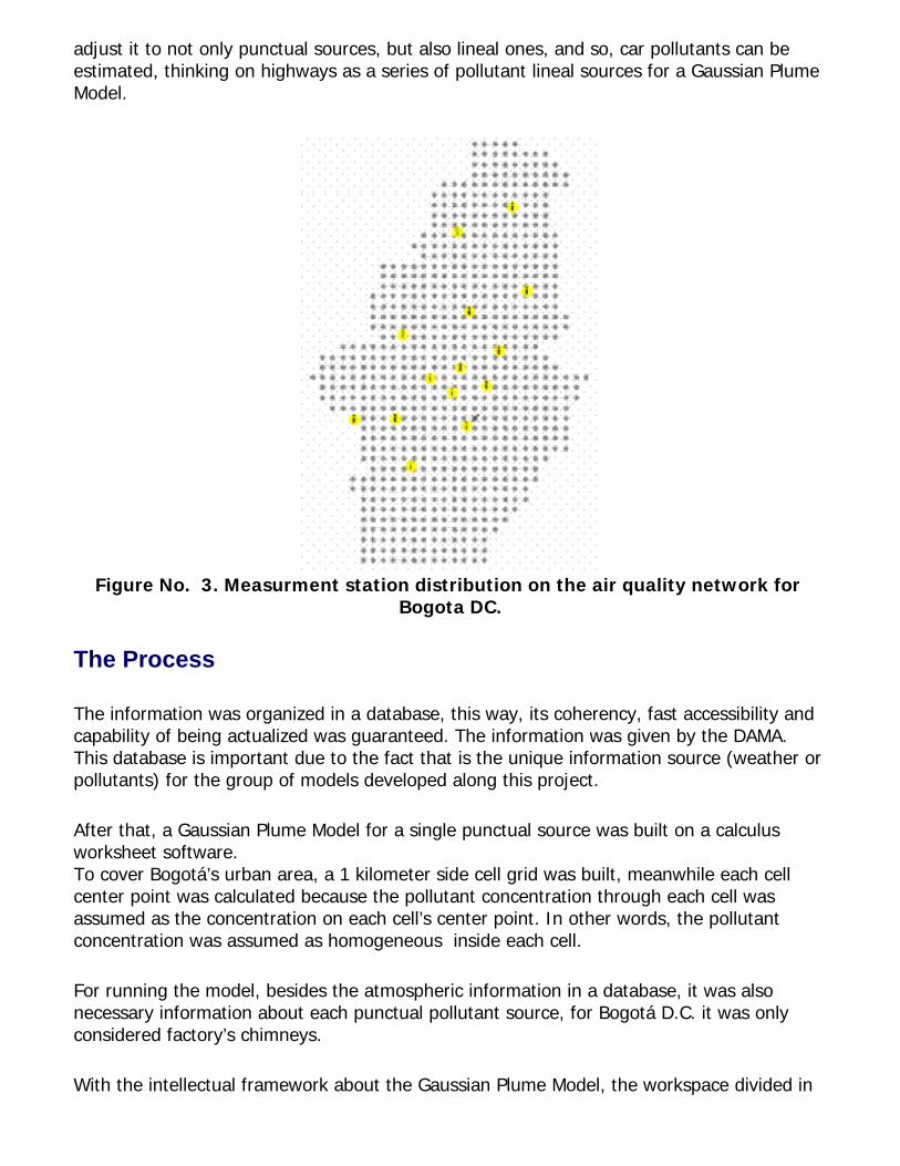
Figure No. 3. Measurment station distribution on the air quality network for

Bogota DC.

The Process

The information was organized in a database, this way, its coherency, fast accessibility and capability of being actualized was guaranteed. The information was given by the DAMA. This database is important due to the fact that is the unique information source (weather or pollutants) for the group of models developed along this project.

After that, a Gaussian Plume Model for a single punctual source was built on a calculus worksheet software.To cover Bogotá’s urban area, a 1 kilometer side cell grid was built, meanwhile each cell center point was calculated because the pollutant concentration through each cell was assumed as the concentration on each cell’s center point. In other words, the pollutant concentration was assumed as homogeneous inside each cell.

For running the model, besides the atmospheric information in a database, it was also necessary information about each punctual pollutant source, for Bogotá D.C. it was only considered factory’s chimneys.

With the intellectual framework about the Gaussian Plume Model, the workspace divided in

a grid, the weather information and the chimney data, the research group was ready for building the model.

THE ISSUES.

The NIDE researchers thought that the issues about the model described below are between the most important things found along this part of the project, because these point out some things that could help to improve the model estimations.

FIRST ISSUE: KIND OF MODEL.

The kind of model used for estimating the air pollutant concentration on a city has a fundamental importance on the results. Each model as an abstraction made from reality, must limit it. For this reason, a model cannot exactly describe the way a phenomenon occurs. So, each model has constraints, advantages and disadvantages over others.

This way, an outstanding Gaussian Plume Model advantage is that this model allows the differentiation among the amount of pollutants which come from static sources (Gaussian Plume Model for punctual sources) and form dynamic sources (Gaussian Plume Model for linear sources), and if a comparison is made between the model’s estimations and the pollutant concentration measured by the air quality network, it is possible to obtain an estimation of air pollutants with non-anthropogenic origin, for instance, particulate matter caused by aerial erosion.

In the same way, the Gaussian Plume Model needs specific information about each source located through the workspace, this implies additional and constant efforts to keep updated information that other models don’t need.

SECOND ISSUE: MODEL LOCATION

The Gaussian Plume Model can be calculated for any X,Y,Z position, however, if it were made in this way, it would need too many arithmetic operations to obtain a full estimation. So, it’s necessary to split the workspace in a grid, to decrease the arithmetic operations needed and obtain a faster model calculation. Besides, the plume has a downwind distribution from the source and this makes unnecessary to estimate pollutant concentrations in the opposite way and so, decrease the number of arithmetic operations.

It’s also neccesary not to forget that air pollution is a problem without administrative boundaries, the pollutants generated by Bogotá goes beyond its limits and pollute the surrounding plateau. So, it’s mandatory to think about the model location in a way that let it integrate into equal or larger scale models with larger workspaces.

THIRD ISSUE: MODEL ORIENTATION .

To estimate, the Gaussian Plume Model uses coordinated axis oriented in a way that the

coordinate origin is in the chimney’s basis and the X axis has the same orientation as the plume axis.

When it’s neccesary to locate a plume in the workspace, it’s also neccesary to orient the model axis according with the workspace axis (for instance, geographic coordinates), keeping always in mind details like the workspace’s geographic projection.

FOURTH ISSUE: AMOUNT OF ARITHMETIC OPERATIONS.

It is notable, specially after reading the second issue, that if it is necessary a high detail level in the pollutant estimation, it is also necessary some time to make the necessary arithmetic operations. Well, the technological development has allowed to improve the amount and speed of calculations with computer’s help, but there are still a lot of natural phenomenon data that could surpass the research team’s technologic capability and so, a real time modelling would be very difficult. This could be a problem if there were an emergency like Mexico City’s air pollutant crisis.

A smaller cell grid or an increase on its coverage implies a larger amount of arithmetic operations to calculate the model, and it is necessary to keep in mind that the air quality network is collecting data each hour, each day, enlarging day by day the database.

FIFTH ISSUE: MODEL TEMPORALITY.

A Gausssian Plume Model constraint is that it works with average time variables, this means that it is necessary that the weather condition data needed by the model must be measured on time intervals from 10 minutes to 1 hour.

The DAMA saves the atmospheric information in an one-hour average format, this could be a constraint with other kind of models, but with Gaussian Plume Model it is OK. This is an important topic on air quality modelling, specially if it is necessary a real time modelling.

In other kind of model’s viewpoint, it is necessary to keep an eye on the time interval in which the weather condition measurements are taken and the time interval in which is possible to keep an acceptable precision level of estimation.

SIXTH ISSUE: PLUME EXTINCTION.

The Gaussian Plume Model was developed from the Gaussian Bell concept and so the model inherited some of its characteristics. One of this characteristics is being asymptotic on one axis. This can be observed on the fact that an plume’s transverse estimation (theoretically) will never reach a zero value.

This way, it is necessary to limit the plume and beyond its limits the concentration is assumed as zero or too small to be considered. A possible way to do this is to state the limitation as an angular value (a transverse limit) because the plume has a conic shape.

It is known that the Gausssian Plume Model estimations are considered exact until 50 km from the source and this is its longitudinal limit. Based on the plume’s limits (transverse and longitudinal), it is possible to decrease the amount of arithmetic operations needed to calculate the model (fourth issue) and this would help on the model improvement.

SEVENTH ISSUE: VARIABLE HOMOGENEITY.

The Gaussian Plume Model assumes that exists homogeneous weather conditions through the plume, this is not completely true on the reality. Is there homogeneous weather conditions through the workspace? The answer for Bogotá DC is negative. This fact is easily confirmed; it is only needed to take a look at the data collected by the air quality network.

This fact made necessary a previous treatment of the weather data, however it is assumed in the model that the weather conditions of the source are the same for the whole plume , but there are still differences between each source’s weather conditions.

How can be obtained the cell’s weather conditions where a source is located? Well, for this purpose was used an interpolation technique called “Inverse Distance Weighted (IDW)” on the air quality network data.

This interpolation technique is well known on earth sciences and it is based on a premise which says that things that are close together are more alike than things farther apart.

In the same way, it is probably that the weather condition differences through the workspace have an important influence on other model’s estimations.

EIGHTH ISSUE: TOPOGRAPHY.

Figure No. 4. Chimney basis height change keeping the chimney’s smokestack

relative height.

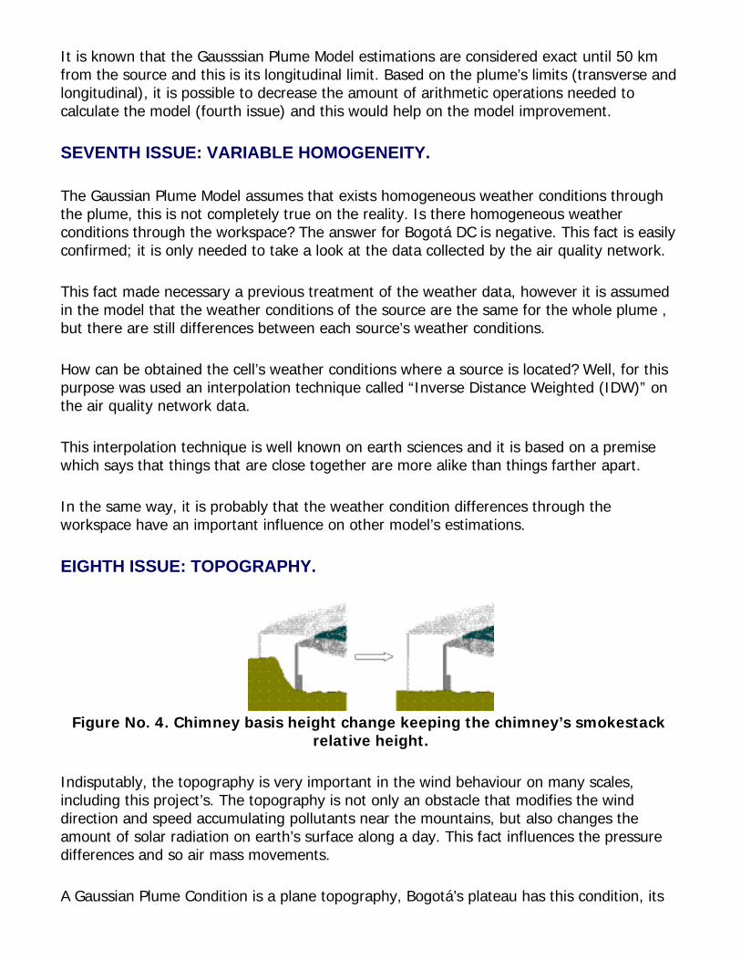
Indisputably, the topography is very important in the wind behaviour on many scales, including this project’s. The topography is not only an obstacle that modifies the wind direction and speed accumulating pollutants near the mountains, but also changes the amount of solar radiation on earth’s surface along a day. This fact influences the pressure differences and so air mass movements.

A Gaussian Plume Condition is a plane topography, Bogotá’s plateau has this condition, its

topography is relatively plane but the exception are the east hills, a Bogotá’s natural limit.

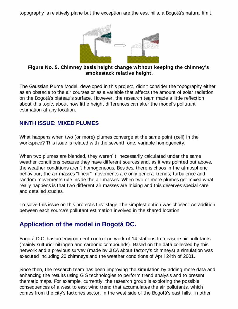
Figure No. 5. Chimney basis height change without keeping the chimney’s

smokestack relative height.

The Gaussian Plume Model, developed in this project, didn’t consider the topography either as an obstacle to the air courses or as a variable that affects the amount of solar radiation on the Bogotá’s plateau’s surface. However, the research team made a little reflection about this topic, about how little height differences can alter the model’s pollutant estimation at any location.

NINTH ISSUE: MIXED PLUMES

What happens when two (or more) plumes converge at the same point (cell) in the workspace? This issue is related with the seventh one, variable homogeneity.

When two plumes are blended, they weren´t necessarily calculated under the same weather conditions because they have different sources and, as it was pointed out above, the weather conditions aren’t homogeneous. Besides, there is chaos in the atmospheric behaviour, the air masses “linear” movements are only general trends; turbulence and random movements rule inside the air masses. When two or more plumes get mixed what really happens is that two different air masses are mixing and this deserves special care and detailed studies.

To solve this issue on this project’s first stage, the simplest option was chosen: An addition between each source’s pollutant estimation involved in the shared location.

Application of the model in Bogotá DC.

Bogotá D.C. has an environment control network of 14 stations to measure air pollutants (mainly sulfuric, nitrogen and carbonic compounds). Based on the data collected by this network and a previous survey (made by JICA about factory’s chimneys) a simulation was executed including 20 chimneys and the weather conditions of April 24th of 2001.

Since then, the research team has been improving the simulation by adding more data and enhancing the results using GIS technologies to perform trend analysis and to present thematic maps. For example, currently, the research group is exploring the possible consequences of a west to east wind trend that accumulates the air pollutants, which comes from the city’s factories sector, in the west side of the Bogotá’s east hills. In other

words, this wind trend takes the city’s industrial zone pollutants to downtown, where the traffic by itself is a serious complication.

Now, some model’s preliminary estimations are going to be shown. It is necessary to have in mind the issues and constraints above mentioned. Remember that the smokestack’s information is not updated and it was taken from a previous study.

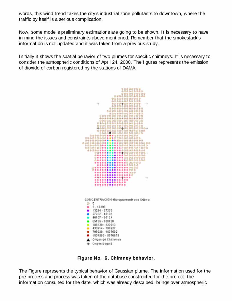
Initially it shows the spatial behavior of two plumes for specific chimneys. It is necessary to consider the atmospheric conditions of April 24, 2000. The figures represents the emission of dioxide of carbon registered by the stations of DAMA.

Figure No. 6. Chimney behavior.

The Figure represents the typical behavior of Gaussian plume. The information used for the pre-process and process was taken of the database constructed for the project, the information consulted for the date, which was already described, brings over atmospheric

variables (temperature, wind speed, wind direction and solar radiation) and the variable in question. It is clearly observed that the wind direction were north - south for the day and the hour specified, provoking that the concentration of dioxide of carbon and in general of all the present pollutants at that moment in the atmosphere went toward the south of the city.

Figure No. 7. Second Chimney behavior.

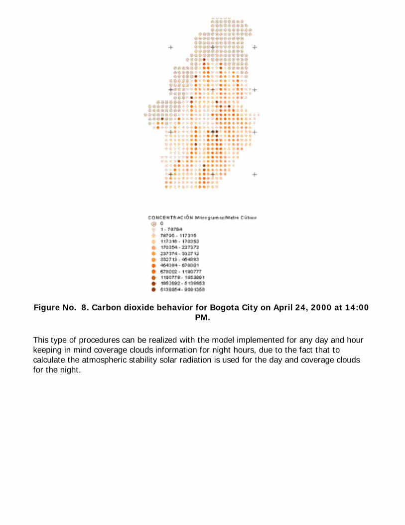
Each of the chimneys, for a specific hour, has different atmospheric conditions and the emission quantity and characteristics are different too. The total concentration was given by the arithmetical add among the resultant concentrations of every estimation on the cell where several plumes converge. Then, having the emissions of all the chimneys and the generated plumes, the behavior of the total concentration of dioxide of carbon for Bogota City on April 24, 2000 at 14:00 is represented as follows.

Figure No. 8. Carbon dioxide behavior for Bogota City on April 24, 2000 at 14:00 PM.

This type of procedures can be realized with the model implemented for any day and hour keeping in mind coverage clouds information for night hours, due to the fact that to calculate the atmospheric stability solar radiation is used for the day and coverage clouds for the night.

Figure No. 9. Gaussian Plume Model estimations for Bogotá, on April 24th of 2002 at 07:00 hours,

calculated 100 meters over the surface.

The points size (cell centers) is proportional to the pollutant concentration; the South – West zone points (and in the following illustration the points on the West zone, the green ones) represent no pollutant concentration because the wind direction predominantly was North – East (On the next illustration, predominantly to the East). This easily discovered by following the largest points (plume’s tracks).

Geostatistical Model.

Some people say that Geostatistics is “the art of modeling spatial data”. Geostatistics is a useful tool for improving estimations of a variable for non-measured locations if it is compared with other estimation techniques, for example IDW (Inverse Distance Weighted interpolation). A more specific definition is that Geostatistics is a statistical methodology used to estimate, forecast, and simulate correlated spatial data, which uses in its analysis exploratory and interpolative methods.

Using Geostatistics for modeling air pollutants behavior in Bogotá has two immediate advantages:

● It is not necessary to collect as much information as it is with the Gaussian Plume Model. The exploratory analysis used the Bogotá’s air quality network data (14

stations taking 24 air pollutant measures a day) for a first approach.● It is not mandatory to collect information about each air pollutant source.For this

reason, it is possible to draw some conclusions faster than with other approaches.

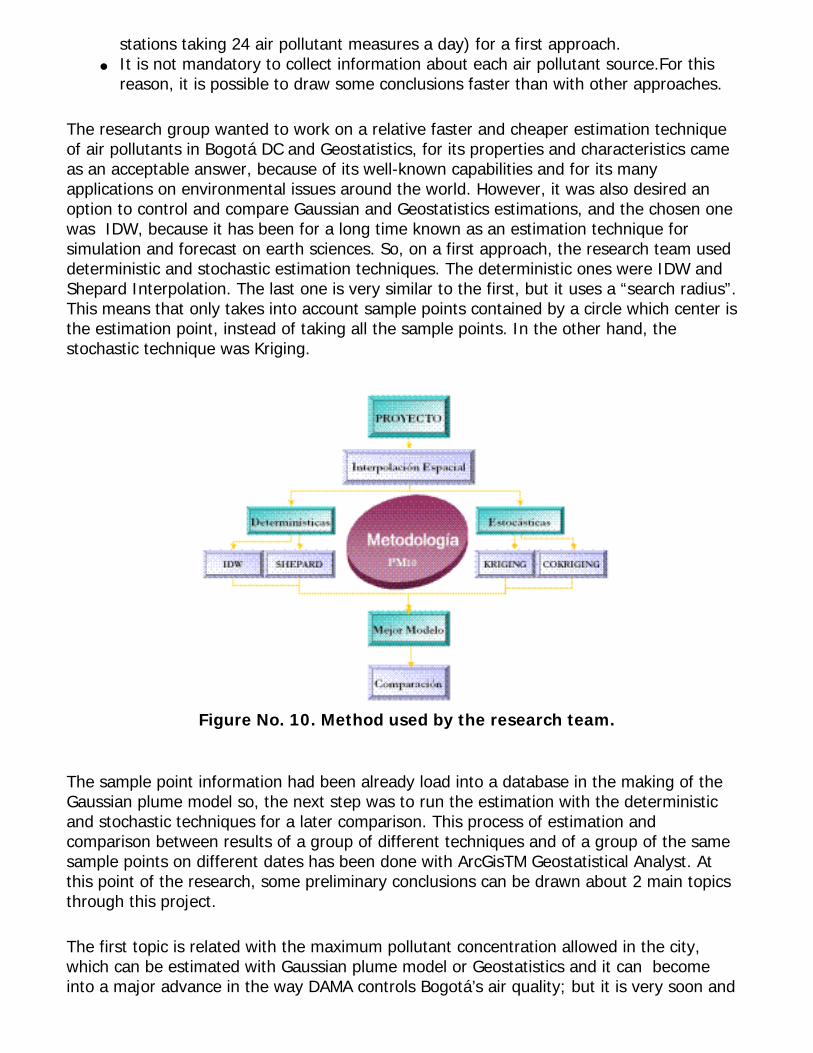
The research group wanted to work on a relative faster and cheaper estimation technique of air pollutants in Bogotá DC and Geostatistics, for its properties and characteristics came as an acceptable answer, because of its well-known capabilities and for its many applications on environmental issues around the world. However, it was also desired an option to control and compare Gaussian and Geostatistics estimations, and the chosen one was IDW, because it has been for a long time known as an estimation technique for simulation and forecast on earth sciences. So, on a first approach, the research team used deterministic and stochastic estimation techniques. The deterministic ones were IDW and Shepard Interpolation. The last one is very similar to the first, but it uses a “search radius”. This means that only takes into account sample points contained by a circle which center is the estimation point, instead of taking all the sample points. In the other hand, the stochastic technique was Kriging.

Figure No. 10. Method used by the research team.

The sample point information had been already load into a database in the making of the Gaussian plume model so, the next step was to run the estimation with the deterministic and stochastic techniques for a later comparison. This process of estimation and comparison between results of a group of different techniques and of a group of the same sample points on different dates has been done with ArcGisTM Geostatistical Analyst. At this point of the research, some preliminary conclusions can be drawn about 2 main topics through this project.

The first topic is related with the maximum pollutant concentration allowed in the city, which can be estimated with Gaussian plume model or Geostatistics and it can become into a major advance in the way DAMA controls Bogotá’s air quality; but it is very soon and

there is too much data to process before stating definitive conclusions.

The second topic is related with an understanding of the interpolation techniques themselves, which is one of the main objectives of the NIDE in this research. Although the research group is still working in this viewpoint, it is possible to draw a preliminary analysis conclusion, which was obtained using cross validation to compare IDW against Geostatistics (Ordinary Kriging) estimation RMS (Root Mean Square error), that applies for Bogotá case and says that it is better to use IDW instead of Geostatistics (Kriging) for estimating air pollution based on the available sample points (air quality stations). The research team thinks that this conclusion is the direct result of the lack of sample points, but it is still necessary to increase the number of estimations to achieve a definitive conclusion.

In this order of ideas, the NIDE is going to continue this research looking for a deeper understanding of the air pollutant behavior on Bogotá DC, and for that reason has already started working on a third modeling approach, with a statistical viewpoint, leaving behind for a little while the geographic component.

Spatial Interpolation

The interpolation is a process that allows to model spatial variables, to predict its behavior, to determine its radiuses of influence and its duration. It also solves decision problems when they are been affected by the behavior of certain variables, and in general, to provide information about either the present or a probable future.

The estimation of unknown values from a sample by means of interpolation is a common practice in many areas of the science, and in fact, they are often inseparable of the processes made in the art of the investigation, especially the related ones with the sciences of the earth. A normal process is to obtain from a sample the general behavior of a phenomenon.

The spatial interpolation is the procedure used to estimate values for one or more variables in places where information neither exists nor it is known from measurement points located in the same area or region. When the estimation of the variables is done in places outside the area covered by the taken measurements, the process is called extrapolation.

The spatial interpolation provides different methodologies to make analysis of spatial information: Geostatistics and Simple Interpolation. Both methodologies can make global or local estimations, they both have exact and approximate interpolators. The difference among these takes root in the suppositions that are assumed by each one, the number of decision parameters and the prediction of the estimation error.

The simple interpolation is based on a natural sciences’ principle from which derives the data continuity, which in a given process the rate of change is constant and at least two values must be known.

The Geostatistics is a statistical technique used for the estimation, prediction and simulation

of information correlated spatially. Its analysis uses exploration and interpolation methods and these methods need a basic statistical knowledge, due to the fact that when there is irregular variation in the information or the simple interpolation shows incoherent results, the Geostatisticals methods provide probabilistic estimations with quality of the interpolation. They provide a tool (semivariograms) that allows to explore and to obtain a better comprehension of the information, besides it grants control over the estimation and this can return the best estimations based on the available information, allowing to take better decisions.

The Geostatistical method is based on the next suppositions: variable stationarity, intrinsic hypothesis and probabilistic distribution in the information. In case that the modeled variable behaves as a normal distribution, the results will be more accurate. The efficiency of this method depends on the uniformity of the area of study.

In general, it is possible to affirm that the geostatistical methods are superior to the simple interpolation if there is a representative sample data and it also depends on the quality of the needed estimation. Due to the fact that in some occasions it is necessary to make predictions outside of the places where information has been taken, sometimes the spatial analysis needs extrapolation, it is supposed that the phenomenon behaves in the same way as the information nearest to the point of estimating.

Kriging and the Semivariogram.

The best Geostatistics’ estimator is Kriging. It is known as BLUE (Best Linear Unbiased Estimator). With Kriging's application it is possible to minimize the variance of the error prediction, since it uses in its estimation the characteristics of variability and spatial correlation of the studied phenomenon.

In Geostatistics, it is very important to mention the spatial correlation, which consists of the estimation of the spatial dependence among the measured information, this process is done through a structural analysis using variograms.

The variograms are variance estimators related to the direction and the distance, they indicate the changes of the spatial dependences that exist among of the origin point and another, independently of its position.

For facility of application of Kriging's equation system, the function of semivariance is used for obtaining the semivariogram. In a set of information, in order to allow to the semivariogram estimate the variance, it is fundamental that the information has certain regularity in its distribution, this means that the information should have some stationarity degree.

In the construction of a semivariogram exists two stages, one is the construction of the experimental semivariogram and the second one is to construct the model of the semivariogram.

The experimental semivariogram is build graphically with the point cloud of distances among the different couples of the samples points, whereas the model of the semivariogram is made through the adjustment of theoretical functions that support the construction of this model. The most useful are the Exponential Model, Spherical Model, Gaussian Model and the Potential Model, whose differences take root in the way the function growth along the range.

The semivariogram is formed by three parameters, Nugget, Sill and Range. The Nugget is the value in which the semivariogram model intercepts the Y axi, this is the semivariance axis, this value can be attributed to measurement errors or spatial variation sources among the samples. The Sill is the top limit of any semivariogram model, the value where the range is reached. The Range is the distance in which the function of semivariance stops growing.

Figure No. 10. Semivariogram’s parameters.The Semivariogram’s parameters are Nugget, Sill y Range.

Once constructed the semivariogram model, it is applied a method of geostatistical interpolation. The method used for this project was Kriging because it minimizes the error variance.

Kriging's objective is to estimate the value of the variable "Z" in a not measured point (Xo). For this, a weightened sum of the weight multiplied by the variable value is made. The basic equation that represents Kriging is:

The Kriging estimation can be punctual or zonal depending on the space in which the variable is going to be estimated. Kriging assembles a set of spatial prediction methods that are based on the minimization of the RMS, actually, they all have the same foundation and differ in the type of estimator (linearly or not linearly), mean value used, trend and the way of avoiding the bias.

After having applied the type of Kriging selected for the phenomenon that is being studied, it is evaluated the kindness of the adjustment of the prediction through a method called cross validation.

Cross validation is based in the exclusion of an observation from the sample points and with the remaining values and the chosen semivariogram model, make a prediction (using Kriging) of the variable value in the exact location of the excluded sample point. If the selected model describes a good structure of spatial auto-correlation, the difference between the estimated and observed value must be minimum, otherwise the model is rejected and the process rethinks.

Methodological scheme for the geostatistical analysis.

In general, to make a good geostatistical analysis it is necessary to make an iterative process to obtain good results. The figure below shows the methodological cycle to execute this type of analysis, which is based on statistical models that include auto-correlation and allows the making of estimations of the phenomena. It is assumed that before making a geostatistical analysis or any another type of analysis, the problem or the phenomenon that is expected to investigate has been defined.

Figure No. 11. Methodological cycle to make an iteration.

In general the methodological scheme for a Geostatistical analysis is described in seven steps.

1. Basic Information. To make a geostatistical analysis, it is necessary to use representative samples of the investigated variable and additional samples to control the obtained results. It is recommended to have a good spatial understanding of the zone or place of the phenomenon location.

2. Select the variables to use. Once selected the variables, it is necessary to choose those that have greater influence on the phenomenon, with a representative amount of samples.

3. Exploratory analysis of the information. Before applying Geostatistics, it is necessary to purify the information to avoid mistakes in the analysis. For example, it is necessary to observe what type of distribution the information has, search if the sample data has some trend, if atypical values exist and decide if they must be included or removed, analyze the spatial distribution and the statistics of the values of the variable.

4. Selection of the method. It must be selected the method that is going to be used to make the interpolation, deterministic (Inverse Distance Interpolation, Inverse Square Distance Interpolation, Shepard Interpolation, Polinomial Interpolation, etc.) or estocastic (Ordinary Kriging, Simple, Universal, Residual, etc) and the variable to be used; it is important to know that it is possible to make both individual or as a whole analysis for the variables, depending on the method of analysis that is in use, Kriging or Co-Kriging.

5. Structural analysis and calculation. The experimental variogram is calculated using a function of spatial correlation, this is the semivariance or covariance, in agreement to the cloud of points generated in the experimental semivariogram, then the theoretical model that better adjusts the experimental semivariogram model is chosen (Spherical, Exponential, Gaussian or Potential). Then it is defined the number and size of the Lags that are going to be in use in the model (it is recommended that the size of the Lag should be similar to the average distance that exists among the spatial location of the information).

It is defined if there is isotropy or anisotropy by means of the semivariogram analysis from different reference angles; with base in the existence or not of directional autocorrelation, it becomes necessary to define the vicinity of analysis for the information and later the monitoring of the prediction mistake is done, which can be made by means of cross validation.

6. Test, Checking and Selection. Different tests are done to choose the best method, deterministic or estocastic, and the best model inside them; in the practice this is to make the steps 4 and 5 many times since it is necessary to find the best model. To choose the most appropriate method depends on the size of the sample and the precision that is required in the prediction. The selection of the best model is based in choosing the one which prediction mistake is minimal. If the results obtained in this stage are not inside the parameters specified in the definition of the problem, it is necessary to to return to step 1, and this means, to improve the sample data and to repeat the analysis cycle.

7. Results. The results can be observed in tables like cross valiadations, histograms, QQPLOTs (it shows the quantiles of the differences among the standardized mistakes and the corresponding quantiles of a normal distribution), trend analysis, clouds of points of the semivariogram or of the covariogram, etc. and maps as those of prediction, probability, prediction of the standard mistake and of quantiles for each of the previous steps.

This process must be repeated for each of the variables that are estimated in the analysis. This methodological scheme is one of the contributions generated by this project, which allows to make the geostatistical analysis in a general form.

Geostatistical model for Bogotá D.C.

Applying the previously explanation for Bogotá D.C. and considering the local considerations, the following processes were executed and the following results were obtained.

USED INFORMATION.

The information used for this stage of the investigation is coincidental with the Database implemented in the initial phase, which contains the DAMA measurements in the period 1997-2000. This Database includes information of the variables that were mentioned previously: pressure, radiation, temperature, rain, wind speed, wind direction, methane, monoxide of carbon, oxides of nitrogen, dioxides of nitrogen, ozone, PM10 and dioxide of sulphur.

DEFINITION AND MEASUREMENT OF VARIABLES.

The variable chosen for the analysis is PM10, this is a solid material that is produced for the wind action on areas without vegetation, materials of the not paved routes, processes of combustion on factories, breaking rocks and for construction materials. The unit in which it is expressed the level of concentration of this variable in the atmosphere is mg/m3.

This variable is selected because it is one of the substances known as a primary pollutant which influences the air quality in cities and besides, from the viewpoint of of human health, it is very interesting because its size does not exceed 10 microns (PM10) and for this reason it can enter to the respiratory tract and produce damages in its organs. In addition, it has been sampled in almost every meteorological station in the study area.

ANALYSYS

The analysis is made on April 24, 2000 and February 13 and April 26, 2001 at 2 p.m., besides it is included February 15, 2002 among 0:00 a.m. and 23:00 p.m. This period is selected for being the date that has more measurements of the variable.

The analysis consists of choosing two or more interpolation methods among the existing ones, to make estimations and to compare the results obtained by each of the selected methods.

It was used a deterministic and stochastic method to make the analysis. The deterministic method selected was Inverse Distance Weightened while the estocastic was Ordinary Kriging. Inverse Distance is selected because it is the simplest method of interpolation, uses few decision parameters and it is a good parameter of comparison. Ordinary Kriging is chosen because uses the sample average.

The stationary of the measured variable is assumed because after making a tested prediction with trend and without it, the error prediction are minor when the calculations are done without it.

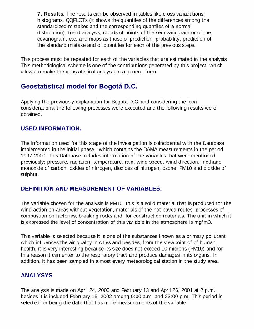
It is done an individual analysis of the variable PM10.

Figure No. 12. Comparison among April 24, 2000 and April 26, 2001.

The above figure compares the distribution of PM10 for April 24, 2000 and April 26, 2001 at the same hour. It is evident, that the distribution for April 26 was more homogeneous and less slanted, besides it is observed how the median of the sample is in half of the variance interval, this means that the distribution is normal. In environmental terms, this means that the distribution of PM10 for April 26, 2001 in Bogota D.C. was uniform in the urban area.

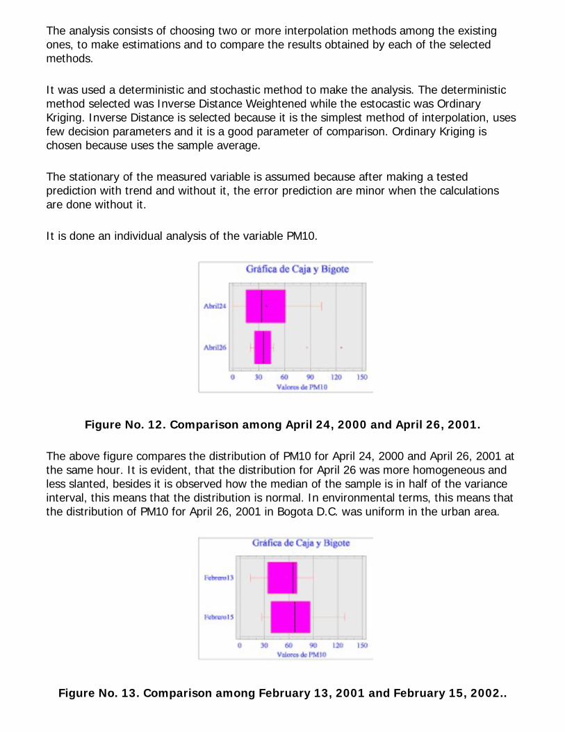
Figure No. 13. Comparison among February 13, 2001 and February 15, 2002..

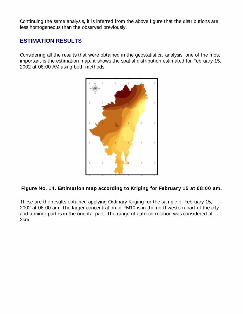
Continuing the same analysis, it is inferred from the above figure that the distributions are less homogeneous than the observed previously.

ESTIMATION RESULTS

Considering all the results that were obtained in the geostatistical analysis, one of the most important is the estimation map, it shows the spatial distribution estimated for February 15, 2002 at 08:00 AM using both methods.

Figure No. 14. Estimation map according to Kriging for February 15 at 08:00 am.

These are the results obtained applying Ordinary Kriging for the sample of February 15, 2002 at 08:00 am. The larger concentration of PM10 is in the northwestern part of the city and a minor part is in the oriental part. The range of auto-correlation was considered of 2km.

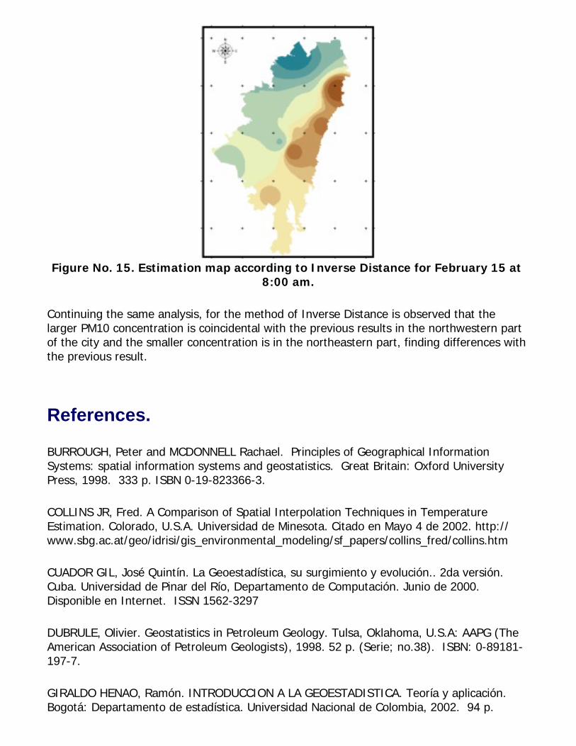
Figure No. 15. Estimation map according to Inverse Distance for February 15 at

8:00 am.

Continuing the same analysis, for the method of Inverse Distance is observed that the larger PM10 concentration is coincidental with the previous results in the northwestern part of the city and the smaller concentration is in the northeastern part, finding differences with the previous result.

References.

BURROUGH, Peter and MCDONNELL Rachael. Principles of Geographical Information Systems: spatial information systems and geostatistics. Great Britain: Oxford University Press, 1998. 333 p. ISBN 0-19-823366-3.

COLLINS JR, Fred. A Comparison of Spatial Interpolation Techniques in Temperature Estimation. Colorado, U.S.A. Universidad de Minesota. Citado en Mayo 4 de 2002. http://www.sbg.ac.at/geo/idrisi/gis_environmental_modeling/sf_papers/collins_fred/collins.htm

CUADOR GIL, José Quintín. La Geoestadística, su surgimiento y evolución.. 2da versión. Cuba. Universidad de Pinar del Río, Departamento de Computación. Junio de 2000. Disponible en Internet. ISSN 1562-3297

DUBRULE, Olivier. Geostatistics in Petroleum Geology. Tulsa, Oklahoma, U.S.A: AAPG (The American Association of Petroleum Geologists), 1998. 52 p. (Serie; no.38). ISBN: 0-89181-197-7.

GIRALDO HENAO, Ramón. INTRODUCCION A LA GEOESTADISTICA. Teoría y aplicación. Bogotá: Departamento de estadística. Universidad Nacional de Colombia, 2002. 94 p.

GORDON S. Thomas. Interactive Analysis and Modelling of Semi-Variograms. Snowden Associates Pty. Disponible en Internet: http://www.ai-geostats.org/online_papers/_papers/0000001e.htm

GUPTILL, Stephen and MORRISON Joel. Elements of spatial data quality. s.l. The International Cartographic Association, 1997. 202 p. ISBN 0-08-042432-5.

ISAAKS, Edward H. and SRIVASTAVA, R. Mohan. Applied Geostatistics. Oxford University Press. 561 páginas. Disponible en Internet: http://www.oup-usa.org/isbn/0195050134.html

JOHNSTON, Kevin. et al. Using ArcGIS™ Geostatistical Analyst, GIS by ESRI™, Disponible en Internet:

http://www.zo.ntu.edu.tw/Courses/GIS/2001-12-05/Using_ArcGIS_Geostatistical_Analyst.pdf

MAJURE, James J. et al. GIS, spatial statistical graphics, and forest health Iowa State University. Disponible en Internet: http://www.public.iastate.edu

MYERS, Donald E. Elements of Geostatistics.. Arizona. Disponible en Internet: http://www.ento.vt.edu/~sharov/PopEcol/lec2/geostat.html

SANCHEZ IPIA, Albert Hamersson y SIABATO VACA, Willington Libardo. Análisis de gases contaminantes en zonas urbanas, Bogotá. Universidad Distrital Francisco José de Caldas. 2002, 83 p. (Serie; Ciencia y Medio Ambiente -Jóvenes Talentos-). ISBN: 958-8175-06-2.

SANCHEZ IPIA, Albert Hamersson y SIABATO VACA, Willington Libardo. Modelo para el análisis del comportamiento de gases contaminantes y material particulado en la zona urbana del altiplano de Bogotá Fase I. Bogotá, 2001, 246 p. Proyecto de investigación (Ingeniero Catastral y Geodesta). Universidad Distrital Francisco José de Caldas. Facultad de Ingeniería.

SANCHEZ IPIA, Albert Hamersson y SIABATO VACA, Willington Libardo. Modelo de calidad del aire para Bogotá, Bogotá D.C. Universidad Distrital Francisco José de Caldas. 2002, p.65-71 ISSN: 0121-750X.

SHARMA, Tara. Spatial Interpolation Techniques in GIS Disponible en Internet: http://www.geog.ubc.ca/courses/klink/gis.notes/ncgia/u40.html

TODA LA TEORIA SOBRE KRIGING. Disponible en Internet: www.ems-i.com/gmshelp/Interpolation/Interpolation_Schemes/ Kriging/Kriging.htm

ULRICH Leopold. Application of Geostatistics for Spatial Analysis of Heavy Metals in Soil. Germany. Soil Science Department, Faculty of Geography and Geo sciences, University of

Trier. Disponible en Internet: http://www.geocities.com/leop6101/abstract.htm

Authors Information.

Adriana Patricia Rangel Sotter.Ingeniera Catastral y Geodesta. Universidad Distrital Francisco José de Caldas. Investigadora Grupo NIDE. asotter@msn.comTel. (+571) 2691607 Cel. 3157962629Instituto Geográfico Agustín CodazziDepartamento de cartografía.

Alber Hamersson Sánchez Ipia.Ingeniero Catastral y Geodesta. Universidad Distrital Francisco José de Caldas. Investigador Grupo NIDE. hamersson@hotmail.comTel. (+571) 2052206 Cel. 3108035147Grupo Empresarial HydrosIngeniero de Soporte y desarrollo.

Jhon William Cely Pulido.Ingeniero Catastral y Geodesta. Msc. Teleinformática. Esp. SIG. Director Grupo de Investigación NIDE. Universidad Distrital Francisco José de Caldas. jwcely@express.net.coTel. (+571) 5482359 Cel. 3108591205Universidad Distrital Francisco Jose de CaldasDirector de Investigaciones de la Facultad de Ingeniería.

Willington Libardo Siabato Vaca. Ingeniero Catastral y Geodesta. Universidad Distrital Francisco José de Caldas. Oracle Certified. Advanced System Admnistrator. Investigador Grupo NIDE. wsiabato@eudoramail.comTel. (+571) 5361310 Cel. 3108035178Grupo Empresarial HydrosIngeniero de Soporte y desarrollo.Insituto de Hidrología Meterología y Estudios Ambientales -IDEAM-Asesor Subdirección Geomorfología y Suelos.