Applied Signal Processing || How could music contain hidden information?

Chapter 7

How could music contain hidden information?

C. Baras (), N. Moreau (*), T. Dutoit (0 )

() GIPSA-lab (Grenoble Image Parole Signal et Automatique), Grenoble, France (*)Ecole Nationale Superieure des Telecommunications, Paris, France CO) Faculte Polytechnique de Mons, Belgium

Why not Attempt To hidE the very pResence of a MessAge in an audio tRacK ?

Audio watermarking started in the 1990s as a modem and very technical version of playing cat and mouse. 1 The music industry, dominated by the "big four" record groups, also known as the "Majors" (Sony BMG, EMI, Universal, and Warner), quickly realized that the availability of digital media for music recordings and the possibility to transfer it fast and degradation-free (thanks to the availability of high data-rate networks and of efficient data compression standards) would not only offer many benefits in terms of market expansion, but also expose their business to a great danger: that of piracy of intellectual property rights. Being able to insert proprietary marks in the media without affecting audio quality (i.e., in a "transparent way") was then recognized as a first step toward solving

1 The real origin of watermarking can be found in the old art of steganography (literally, "hidden writing", in ancient Greek). Although the goal of cryptography is to render a message unintelligible, steganography attempts to hide the very presence of a message by embedding it into another information (Petitcolas et al. 1999)

T. Dutoit, F. Marques (eds.), Applied Signal Processing, DOl 10.1007/978-0-387-74535-0_7, ©Springer Science+Business Media, LLC 2009

224 C. Baras, N. Moreau, T. Dutoit

this issue. Additionally, ensuring the robustness of the proprietary mark to not only to usual media modifications (such as cropping, filtering, gain modification, or compression) but also to more severe piracy attacks quickly became a hot research topic worldwide.

Things changed radically in 2007 (i.e., before audio watermarking could be given a serious commercial trial). As a matter of fact, the digital rights management (DRM) employed by the Majors to restrict the use of digital media (which did not make use of watermarking techniques) became less of a central issue after the last Majors stopped selling DRMprotected COs in January 2007 and after S. Jobs' open letter calling the music industry to simply get rid of DRM in February of that same year (Jobs 2007).

Audio watermarking techniques are now targeted to more specific applications, related to the notions of "augmented content" or "hidden channel." One such application is audio fingerprinting, 2 in which a content -specific watermark is inserted in the media and can thus be retrieved for the automatic generation of the playlist of radio stations and music television channels for royalty tracking. Audio watermarking has also been proposed for the next generation of digital TV audience analysis systems; each TV channel would insert its own watermark in the digital audio and video streams it delivers, and a number of test TV viewers would receive a watermark detection system connected to a central computer. 3

In the next section, we will first introduce the principles of spread spectrum and audio watermarking (Section 7.1). This will be followed by a MA TLAB-based proof of concept, showing how to insert a text message in an audio signal (Section 7 .2) and by a list of pointers to more advanced literature and software (Section 7.3).

2 The terrnfingerprinting is also used in the literature for specifying the technique that associates a short numeric sequence to an audio signal (i.e., some sort of hashing; Craver et al. 2001). We do not use it here with this meaning.

3 With analog TV, audience analysis is much simpler; since each TV channel uses a specific carrier frequency, measuring this frequency through a sensor inserted in TV boxes gives the channel being watched at any time. This is no longer possible with digital TV, since several digital TV channels often share the same carrier frequency, thanks to digital modulation techniques.

How could music contain hidden information? 225

7.1 Background- Audio watermarking seen as a digital communication problem

Watermarking in an audio signal can be seen as a means of transmitting a sequence of bits ("1 "s and "O"s) through a very particular noisy communication channel, whose "noise" contribution is the audio signal itself. With this view in mind, creating an audio watermarking system amounts to designing an emitter and a receiver adapted to the specificities of the channel; the emitter has to insert the watermark in the audio signal in such a way that the watermark cannot be heard, and the receiver must extract this hidden information from the watermarked audio signal4

(Fig. 7.1).

Audio signal

I • Watermark J Emitter I J Channel

L Watermarked J Receiver I Watermark'

signal

Watermark Watermark encoder decoder

Fig. 7.1 Audio watermarking seen as a communication problem

The problem therefore looks very similar to that of sending information bits through the Internet with an ADSL connection; one has to maximize the bit rate while minimizing the bit error rate, even in the presence of communication noise and distortion.5 In other words, watermarking directly benefits from 50 years of digital communication theory, after the pioneering work of Claude Shannon.

However, watermarking techniques are very specific in terms of bit rate, error rate, and signal-to-noise ratio. SNR is typically made very low so as to make the watermark inaudible. This results in very low bit rates (several hundred bits per second at best) and high error rates (typically 10-3), as opposed to the megabits per second of ADSL modems and the associated low error rates (10-6). In that respect, watermarking techniques are closer

4 This is often referred to as blind watermarking, in which the receiver has no a priori information on the audio signal.

5 Watermark distortion is typically produced by filtering and encoding operations applied to the audio signal while being transmitted, such as MP3 encoding.


to those used for communication between interplanetary satellites and earth. In particular, spread spectrum techniques are used in both cases.

Spread spectrum signals will be reviewed in Section 7.1.1. In the next sections, we will consider the emitter/receiver design issues in a blind (Section 7.1.2) and informed watermarking system (Section 7.1.3) respectively.

7.1.1 Spread spectrum signals

Spread spectrum communications (Peterson et al. 1995) were originally used for military applications,6 given their robustness to narrowband interference, their secrecy, and their security. As a matter of fact, spread spectrum signals are characterized by two unique features: 1 . Their bandwidth is made much wider than the information bandwidth

(typically 10-100 times for commercial applications; 1,000 to 106

times for military applications). The spread of energy over a wide band results in lower power spectral density (PSD), which makes spread spectrum signals less likely to interfere with narrowband communications. Conversely, narrowband communications cause little to no interference to spread spectrum systems because their receiver integrates over a very wide bandwidth to recover a spread spectrum signal. As we shall see below, another advantage of such a reduced PSD is that spread spectrum signal PSD can be pushed on purpose below communication noise, thereby making these signals unnoticeable.

2. Some spreading sequence (also called spreading code or pseudonoise) is used to create the wide-band spread spectrum signal from the information bits to send. This code must be shared by the emitter and the receiver, which makes spread spectrum signals hard to intercept.

The price to pay for these features is a reduced spectral efficiency, defined as the ratio between the bit rate and the bandwidth; the number of bits per second and per hertz provided by spread spectrum techniques is typically less than 1/5, while "standard" techniques offer a spectral efficiency close to 1 (Massey 1994 ).

In the 1990s, spread spectrum techniques have found a major application in code division multiple access (CDMA), now used in satellite positioning systems (GPS, hopefully in Galileo), and for wireless digital phone communications systems (UMTS).

6 Spread spectrum communications dates back to World War II.


Direct sequence spread spectrum (DSSS)

Common spread spectrum systems are of the time hopping (also called direct sequence) or frequency hopping type. In the latter case, as its name implies, the carrier of a frequency hopping system hops from frequency to frequency over a wide band, in an order defined by the spreading code. In contrast, direct sequence spread spectrum (DSSS) signals are obtained by multiplying each bit-sized period (of duration Th) of the emitted signal (the watermark signal in our case) by a (unique) spreading sequence composed of a random sequence of ±1 rectangular pulses (of duration T) (Fig. 7.2, left).

a

t ~lllliiilliill1l ~ 0,2 0.4 0.. 0.1 1 1.2

Tlme(a) - 211 - 10 0 10 ,.,...,...,cy (tU)

Fig. 7.2 Left: Emitted signal, spreading sequence, and spread signal waveforms for Tb=0.2s and T.=T/16. Right: PSD of the input signal compared to that of the spread signal for T,=T,/4 and T,=T/16

It is easy to compute the PSD of such a spread spectrum signal if we assume that the emitted signal is a classical NRZ random binary code composed of rectangular pulses of duration Tband of amplitude ±liTh. As a matter of fact, the PSD of such a signal is given by

S NRZ (f) = _!_Sine 2(!1;,) T,

(7.1)

and since the spread signal is itself an NRZ signal with pulse duration T,. and pulse amplitude±l/Tbits PSD is given by the following equation

S ,pread (f) = i 2 sine 2(f1'c) b

(7.2)


Both PSDs are plotted in Fig. 7.2 (right) for two values of T,. Clearly, when T, decreases, the bandwidth of the spread signal increases, and its maximum PSD level decreases accordingly.

As mentioned above, the resulting spread spectrum signal offers an increased robustness to narrowband interference and distortion; while a low-pass filter with cutoff frequency of 5 Hz would almost completely delete the input NRZ signal, its effect on the spread signal would be mild. Spread spectrum techniques also make it possible to hide information in communication noise, as suggested in Fig. 7.2 (right) with a background noise of unitary variance.

7.1.2 Communication channel design

In this section, we will discuss emitter and receiver design issues and estimate the corresponding bit error rate.

Emitter

We will use the notations introduced in Fig. 7.3; the audio signal x(n), sampled at F, Hz, is added to a spread spectrum watermark signal v(n) obtained by modulating a watermark sequence of M bits b m (in { 0, I } ) with a spreading signal c(n) composed of N, samples (and shown in Fig. 7.3 as a vector c=[c(O),c( 1 ), ... ,c(N" -1 )]\

x(n) ------~

g

Emitter Channel Receiver

Received bits

Fig. 7.3 A more detailed view of a watermarking system seen as a communication system with additive channel noise

Vector c is synthesized by a pseudo-random sequence generator as a Walsh-Hadamard sequence or a Gold sequence with values in {- I,+ 1}.


Following the time-hopping principle exposed in the previous Section, the spread spectrum signal v(n) is given by

M-1

v(n)= 'L.amc(n-mNb) (7.3) m=O

where am is a symbol in { -1 ,+ 1} given by am=2bm-l. One can also see this signal as a concatenation of vectors:

{ +c if am= 1

v =a c= m m -c zif a = -1

m

(7.4)

It is finally amplified by some gain g, which makes it possible to control the signal-to-noise ratio (SNR) between the watermarked signal v(n) and the audio signal x( n ).

Since 1 bit is emitted every Nh samples, the bit rate is simply given by R=F/Nb (bits/s), where F,is the sampling frequency (typically 44.1 kHz).

Receiver

In the case of the additive white Gaussian noise (A WGN) channel shown in Fig. 7.3, the signal y(n) available at the receiver is a noisy version of the emitted signal v(n), with channel noise PDF given by N(O,o""/).

We will further assume that the received samples y(n) are perfectly synchronized with the emitted samples x(n), i.e., the received samples can be organized in vectors .Ym=[y(mNb), y(mNb+l), ... , y(mNb+Nb-l)f related to vectors .Em by

- = { + gc + xm if am = 1 Ym -gvm +xm .

-gc+xm if am =-1 (7.5)

where xm=[x(mNb), x(mNb+l), ... , x(mNb+Nb-l)f is a vector of channel noise samples and m is the frame index.

Since the modulation operation is assimilated to raw concatenation,? and thereby produces no symbol interference, symbol detection can be performed on a symbol-by-symbol basis (no Viterbi algorithm is needed). The optimal detector in this case is the maximum a posteriori (MAP) detector (Proakis 2001),8 which maximizes the probability of each received

bit bm, given the corresponding received vector y m:

7 This is the simplest possible case of a memory less linear modulation scheme. 8 The same as the one used in Chapter 4 for vowel classification.


b m = arg max P( b I y m) bE{O.l}

In the next paragraphs, we will show that this is equivalent to estimating

bm from the sign of the normalized scalar product am between the received

vector y m and the spreading code c:

(7.7)

As a matter of fact, following the same development as in Chapter 4, Section 4.1, Equation (7.6) is equivalent to

b m = arg max P(y m I b )P( b) bE{O.l} P(ym) (7.8)

= arg max P(y m I b )P( b) bE{O.l}

in which P(y J is the a priori probability of y m' which does not influence

the estimation of bm, and P(b) is the a priori probability of each possible

value of b. Furthermore, if the symbols have the same probability of occurrence, Equation (7.8) reduces to

b m = arg max P(y m I b) bE{O.l}

(7.9)

known as the maximum likelihood decision. In the A WGN channel case, since xm is an Nb-dimensional multivariate

Gaussian random variable with zero mean and covariance matrix equal to CY,2I (where I is the Nb-dimensional unity matrix), Equation (7.5) shows that y m is also a multivariate Gaussian random variable, with mean equal to a,gc and the same covariance matrix as xm. Hence

(7.10)

9 In the sequel, we use the same shortcut notation for probabilities as in Chapter 4; P(alb) denotes the probability P(A=aiB=b) that a discrete random variable A is equal to a, given the fact that random variable B is equal to b will simply be written, or the probability density pA,Bob (a) when A is a continuous random variable.


It follows that

b m = arg min II y m - ( 2b - 1) gc II 2

bE{O,Il

= arg min (II y m 11 2 - 2 < y m, (2b -l)gc > +(2b -1)211 C 11 2 ) (7 .11) bE{O,I}

= argmax < y m,(2b-l)gc > bE{O.I }

since (2b-l )2= 1, whatever be the value of b in { 0,1 } . In other words, as

mentioned, bm is obtained from the sign of the scalar product <y m c>, i.e.,

from the sign of am:

b = - {0 m 1

if<ym,c>~O

if<ym,c>>O (7.12)

Fig. 7.4 shows a synthetic view of Equation (7.9) in the case bm is "1." - -

In the left plot, bm ="1," while the right plot will wrongly result in bm ="0" .

... ---•

c.L

<X,C> C gc II ell'

oc gc o c ,

Decision= "0": Decision= "I" I

Decision= "0": Decision= "1"

Fig. 7.4 Watermarking of audio vector x with symbol "1." Watermarked vector y is obtained by adding gv (i.e., gc, given the symbol is "1") to x. Symbol "1" will be detected if a 2 0. Left: Since <x,c> is positive, any (positive) value of g will result in a 2 0. Right: Since <X,c> is negative, only a value of g 2 <x,c>/llc 112 will result in a2 0 (this is not the case in the figure)


Error rate

The PDF of a;., for g set to I and O"/ set to 20 dB is given in Fig. 7.5 for various vector lengths N", i.e., for various bit rates R.

Projecting Equation (7 .5) on the spread sequence c, the scalar product a;., appears as a one-dimensional Gaussian random variable with mean

(2b"'-l )g and variance a~ /II c 11 2 • The latter is that of the normalized

scalar product between the N"-dimensional multivariate Gaussian random variable x and c. Hence

m

1 ( a - (2b -l)g J P( a I b ) = exp - m m

m Ill &ax/llc ll 2a~ /1 1 cll2 (7.13)

As expected, the probability of a;., to be positive while b"'=O and the related probability of a;., to be negative while b"'= l are nonzero, and these values increase with R (i.e., when N" decreases). The probability of error is given by the following equation:

?, =P(b = 1)P(a~ 01 b = 1)+ P(b =O)P(a> 0 I b = 0)

1.2

~ ·~ .g 0 .6

~ ~ o.e ...

..0 £ 0.4

0.2

a

-R:50 ···· · R:lOO --- R:120

(7. 14)

Fig. 7.5 Probability density functions for a when b=O and I for various values of the bit rateR (and with F,=44, I 00, ,R= I, eJ..2 =20 dB)

When symbols have the same a priori probability, this probability of error can be estimated in Fig. 7.5 as the area under the intersection of P( a)b"' =0) and P( a;,,b,= I). It is also possible to compute P,. analytically (Proakis 2001), which leads to


P,. =Q g 2 =Q -Lg / with Q(u)= f--exp -- dt (

211 c 11

2) ( F 2a 2

] ~ 1 ( t2)

ax R ax "J21i 2 (7.15)

in which we have used a/= II c 11 2 /Nb, an estimate of the power of the

spreading sequence. The probability of error is thus finally a function of the watermarking

SNR (i.e., the ratio between the power of the emitted signal, g2ac2, and that of the audio signal, a/) and of the bit rate R. Figure 7.6 shows a plot of

Q( .Ju) and the resulting plot of P,(R) for various values of the SNR. It

appears that P,.= I 0-3 can be reached with a bit rate of 50 bits/s and a SNR of -20 dB. As we will see below, this SNR approximately corresponds to a watermark just low enough not to be heard (or, consequently, to the kind of SNR introduced by MPEG compression; see Chapter 3).

a ,r1 !;!':! :H!,!U!~i!~:':'!ii!!:i::!:i!iiii'!i:i:i!ii! i'Ei:l!iii'!!'i'

.•.•• - ~ · · .,. ··- ····- · I·• .••• -· •·\· ·-· ·• .•• :; ... , •• • •• •Y.• • ,, ,, ,,

...• . •.•..• ...• .. •. · ·!· · ••.•.• , .. ' ···•-'!·"··· ·····~ ·· · · ···· · · - -.. : ... .. . .. ~.. .. . ... : .. ".. . . : -. ' ... .

10 ... : :~!l! ~~1:: :: :::. m H:i: P! ~ ;~l !!:i!! !l ! !l!m imHl!Hl!im~!n! g; :::::: ::::: !:: :::::::: ... ~ -:: ;: :::: ~: ::: ~:::: :: != :::::::::: ~::::: =: ::: ' • ' ' • 0 ' •• ' • • ! o • 1 • • • • o -~ I• o • • ~- o • o o ' '' • o ;:, 'o ''I • •• '• .:. ' • ' • •• "'

} ,D~ ;.;;;i;i!;;j;;.i•i;;;;:,,;,;;;:;;;,l:::;;:,;::·!:;;;:,;;;;[l:;i!;;;;;;: :·:::: :: :::;::::· ::: ·::;;:·:::·:::: ~: :·: · : :::::~:. ·::::::r:::::::::· ···········1·· ·········1· ····· ..... ............ , ....... .............. .

,o_. ~: H l ~ H :~ ~~ l1 'E i:~ ~ ii ~ ; H~ ~ ~ :~ :t ~l m Hi i lit ~1 l~ H: l H :: ~·: H l m [~ i ;::.:: ::::;j;;:::::::: .j::::::::.::(: ::: ::.::.:;::: :::::::.~ .. ·: .::.:. :::::: :::::;::: :: : ::~ : : ~: :::::::::: ~:: ::::::::: r :::::::::: r: :. -.. : :::

,0 ... 0~----:.~~.~~.:---~.:--~:--~ U(dB)

b

Fig. 7.6 Left: Q ( .Ju) with u in dB; right: PJR) for various values of the SNR

and F,=44, l 00

7.1.3 Informed watermarking

Although it is generally not possible to adapt the encoder to the features of the channel noise, 10 such a strategy is perfectly possible in watermarking systems, as the communication noise itself is available at the encoder. In other words, watermarking is a good example of a communication channel with side information (Shannon 1958, Costa 1983). This opens the doors to

10 In some communications systems (like in ADSL modems), the communication SNR is estimated at the receiver and sent back to the emitter through a communication back channel.


the second generation of watermarking systems: that of informed watermarking (Cox et al. 1999, Chen and Wornell 2001, Malvar and Florencio 2003) and its triple objectives; maximal bit rate, minimal distortion, and maximal robustness. In the next paragraphs, we will consider two steps in this direction: gain adaptation and perceptual filtering.

Gain adjustment for error-free detection

The most obvious way to turn the encoder into an informed encoder is to adapt the gain g as a function of time so as to compensate for the sudden power variations in the audio signal and keep the SNR constant. This can be achieved by estimating a/ on audio frames (typically 20 ms long, in which music is assumed to be stationary) and imposing g to be proportional to ax.

It is also possible, and more interesting, to adjust g to impose error-free detection (Malvar and Florencio 2003, LoboGuerrero et al. 2003). As we have seen in the previous section indeed, the probability of error can be made as small as we want by shifting apart the Gaussians in Fig. 7.5, i.e., by increasing g. It is even possible to obtain error-free detection by adapting the gain to each frame (hence we will denote it as gJ so as to yield

(7.16)

As seen in Fig. 7.4, this condition is automatically verified for any (positive) value of g"' if /3"' has the same sign as a,. In the opposite case, it is verified by imposing gm = -j3)a"'.

In practice though, the transmission channel itself will add noise to the watermarked vector y m' leading to received vectors equal to y m +Pm· Condition (7 .16) becomes

(7.17)

Some security margin ~8 is then required to counterbalance the projection ofpmonc(Fig. 7.7):


if am= 1

if am= -1 (7.18)

The value of ~g is set according to the estimated variance of the transmission channel noise.

- -i -------- -----

Fig. 7.7 Informed watermarking of audio vector x with symbol "1." Watermarked vector y is obtained by adding gv (i.e., gc, given the symbol is "1") to x, with g chosen such that y falls in the gray region, where decision will be "1." Two cases are shown: for x''', g can be set to zero; for x"', g must have a high value. The gray region has been shifted from the white region by a 2L\-wide gap to account for possible transmission channel noise

The efficiency of this watermarking strategy stems from the fact that the gain g is directly proportional to the correlation between the audio signal x and the spread sequence c. However, it does not ensure the perceptual transparency of the watermark: in case x is very much in the opposite direction of c while the emitted symbol is "1" (as it is the case of x2 in Fig. 7.7), g must be set to a high value. In such a case, chances are that the watermark may significantly distort the audio signal.

Perceptual shaping filter

A solution to the perceptual transparency requirement is to use properties of the human auditory system to ensure inaudible watermarking. As we have shown in Chapter 3, psychoacoustic modeling (PAM) has established the existence of a masking threshold, assimilated to a PSD cf>(j) (see Chapter 3, Sections 3.1.3 and 3.1.4) below which the PSD of the


watermark Sw (f) must lie for making it inaudible. This threshold is

signal-dependent and must therefore be updated frequently, typically every 20ms.

Since the efficiency of a watermarking system is a function of the SNR ratio (Fig. 7.6), the best performance is reached when

(7.19)

This can be achieved, as shown in Fig. 7 .8, by replacing the scalar gain g by a perceptual shaping filter G(j), which is conveniently constrained to be an all-pole filter:

b G(z) =I -1 ~2 -p

+a1z +a2z + ... +aPz (7.20)

If the input v(n) of this filter is assimilated to white noise (with zero mean and unity variance), adjusting the coefficients of this filter so that its

output w(n) will have a given PSD Sw (f) is a typical filter synthesis

problem, which has already been examined in Chapter I. It is based on solving a set of p linear equations, the so-called Yule- Walker Equations (1.5), whose coefficients are the first p values of the autocorrelation

function ¢w(k) ofw(n). These values are related to the PSD ofw(n) by the

inverse discrete-time Fourier transform formula

1/2

r/J,. ( k) = J <l>(f)eJ2!tfk df (7 .21) -1/2

which can be approximated by an inverse discrete Fourier transform using N samples of <I>(j):

rpjk) =__!__I: <I>(!!_) ei~nk N n=O N

(7.22)

The receiver has to be modified accordingly (Fig. 7.8) by inserting an inverse, zero-forcing equalizer 1 I G(f) before the demodulator (Larbi

et al. 2004). However, since the audio signal x(n) used to derive G(j) is not available at the receiver, an estimate I I G(f) is computed by

psychoacoustic modeling of the watermarked signal y(n). The accuracy of this estimation depends on the robustness of the PAM to the watermark and to possible transmission channel noise, such as MPEG compression.


This specific constraint on the PAM used in watermarking distinguishes it from the PAMs used in audio compression (such as in MPEG).

Ernitt<r Channel Receiver

Received bit>

Fig. 7.8 Informed watermarking using a psychoacoustic model (PAM), a perceptual shaping filter G(f), and a Wiener equalizer H(f)

Once perceptual shaping has been inverted, detection is achieved as previously, except that it is based on estimating the sign of <zm,c>, where z(n) is the output of the inverse filter. Assuming 1 I G(f) is close enough to

1 I G(f), zm is given by

(7.23)

where r(n) is the audio signal x(n) filtered by 1/ G(f). Equation (7.23)

simply replaces Equation (7 .5).

Wiener filtering

As we will see in Section 7.2.3, the SNR at the output of the zero-forcing equalizer is very low; the power of the spread spectrum signal v(n) is small compared to that of the equalized audio signal r(n). Since the PSDs of v(n) and r(n) are different, it is possible to filter z(n) so as to increase the SNR, by enhancing the spectral components of z(n) dominated by v(n) and attenuating those dominated by r(n). This can even be done optimally by a symmetric FIR Wiener filter H(z) at the output of the zero-forcing equalizer (Fig. 7.8):

p

H(z) = L h(i)z-; (7.24) i=- p


The output of the FIR Wiener filter H(z) is made maximally similar to v(n) in the minimum mean-square-error (MMSE) sense (Fig. 7.9); its coefficients are computed so as to minimize the power of the error signal e(n)=z(n)-v(n). It can be shown (Haykin 1996) that this condition is met if the coefficients h(i) of the filter are the solution of the so-called WienerHop! equations:

t/Jzz (0} t/Jzz (1} r/J __ (2 p) h_f! ¢,)-p)

t/Jzz(-1} t/Jzz (0} t/Jzz (2 p -1) h_p+l ¢,.,. (-p + 1) (7.25)

t/JzJ-2p) t/Jzz(-2p+ 1) t/Jzz(O) hf! t/JV\ ( p)

where ¢zz(k) and r/J"'(k) are the autocorrelation functions of z(n) and v(n),

respectively.

z(n) o----+1 H(z)

h(i)

1\ 1------.----+0 v(n)

MMSE ._!!!!!)_ +

+

~~®-----------~

Fig. 7.9 Conceptual view of a Wiener filter 11

In practice, since r(n) is not stationary, the Wiener filter is regularly adapted.

7.2 MATLAB proof of concept: ASP _watermarking.m

In this section, we develop watermarking systems whose design is based on classical communication systems using spread spectrum modulation. We first examine the implementation of a watermarking system and give a brief overview of its performance in the simple and theoretical

11 In practice, v(n) is not available. Nevertheless, only its autocorrelation is required to solve the Wiener-Hopf equations.


configuration where the audio signal is a white Gaussian noise (Section 7 .2.1 ). Then we show how this system can be adapted to account for the audio signal specificities, while still satisfying the major properties and requirements of watermarking applications (namely inaudibility, correct detection, and robustness of the watermark); we extend the initial system by focusing on the correct detection of the watermark (Section 7 .2.2), on the inaudibility constraint (Section 7.2.3), and on the robustness of the system to MP3 compression (Section 7.2.4).

7.2.1 Audio watermarking seen as a digital communication problem

The following digital communication system is the direct implementation of the theoretical results detailed in Section 7 .1. The watermark message is embedded in the audio signal at the binary rate of R=lOO bps. To establish the analogy between watermarking system and communication channel, the audio signal is viewed as the channel noise. In this section, it will therefore be modeled as a white Gaussian noise with zero mean and variance si gma2_x. si gma2_x is computed so that the signal-to-noise ratio (SNR), i.e., the ratio between the watermark and the audio signal powers, is equal to -20 dB.

Emitter/Embedder

Let us first generate a watermark message and its corresponding bit sequence.

message = 'Audio watermarking: this message will be embedded in an audio signal, using spread spectrum modulation, and later retrieved from the modulated signal.'

bits= dec2bin(message); %converting ascii to 7-bit string bits= bits(:)';% reshaping to a single string of l's and O's bits = double(bits) - 48; %converting to a O's and l's symbols = bits*2-1; %a (lxlOSO) array of -l's and +l's N_bits = length(bits);

message =

Audio watermarking: this message will be embedded in an audio signal, using spread spectrum modulation, and later retrieved from the modulated signal.

We then generate the audio signal, the spread spectrum sequence, and the watermarked signal. The latter is obtained by first deriving a symbol sequence ( -1 's and + 1 's) from the input bit sequence (0' s and + 1 's) and then by modulating the spread spectrum signal by the symbol sequence


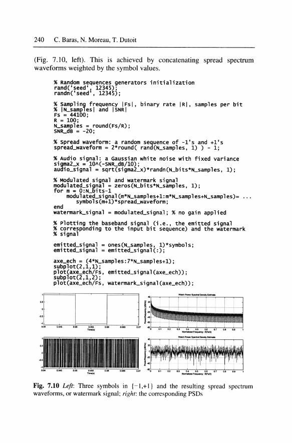
(Fig. 7.1 0, left). This is achieved by concatenating spread spectrum waveforms weighted by the symbol values.

% Random sequences generators initialization rand('seed' 12345); randn('seed 1, 12345);

%Sampling frequency IFsl, binary rate IRI, samples per bit % IN_samplesl and ISNRI Fs = 44100; R = 100; N_samples = round(Fs/R); SNILdB = -20;

% Spread waveform: a random sequence of -1's and +1's spread_waveform = 2*round( rand(N_samples, 1) ) - 1;

%Audio signal: a Gaussian white noise with fixed variance sigma2_x = 10A(-SNILdB/10); audio_signal = sqrt(sigma2_x)*randn(N_bits*N_samples, 1);

% Modulated signal and watermark signal modulated_signal = zeros(N_bits*N_samples, 1); for m = O:N_bits-1

modulated_signal(m*N_samples+1:m*N_samples+N_samples)= symbols(m+1)*spread_waveform;

end watermark_signal = modulated_signal;% no gain applied

%Plotting the baseband signal (i.e., the emitted signal % corresponding to the input bit sequence) and the watermark % signal

emitted_signal = ones(N_samples, 1)*symbols; emitted_signal = emitted_signal(:);

axe_ech = (4*N_samples:7*N_samples+1); subplot(2,1,1); plot(axe_ech/Fs, emitted_signal(axe_ech)); subplot(2,1,2); plot(axe_ech/Fs, watermark_signal(axe_ech));

Fig. 7.10 Left: Three symbols in { - 1 ,+I } and the resulting spread spectrum waveforms, or watermark signal; right: the corresponding PSDs


As expected, the power spectral density (PSD) of the spread spectrum sequence (i.e., the watermark signal) is much flatter than that of the baseband signal (i.e., the emitted signal) corresponding to the input bit sequence (Fig. 7.1 0, right), while their powers are identical: 0 dB.

power_baseband_dB=10*log10(var(emitted_signal)) power_spread_spectrum_dB=10*log10(var(watermark_signal))

subplot(2, 1, 1) pwelch(emitted_signal,[],[],[],2);12 subplot(2,1,2) pwelch(watermark_signal,[],[],[],2);

power_baseband_dB = -0.0152 power_spread_spectrum_dB = 5.5639e-006

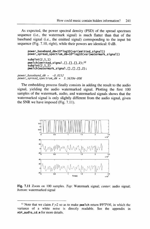
The embedding process finally consists in adding the result to the audio signal, yielding the audio watermarked signal. Plotting the first 100 samples of the watermark, audio, and watermarked signals shows that the watermarked signal is only slightly different from the audio signal, given the SNR we have imposed (Fig. 7.11 ).

:~~ l 0 0.5 , 1.!5 2 2.5

~t~~l~~ l 0 ~ 1 u u

x IO..l

40r-----.-----.---....---......... -----,

2: \ ~,JJV\~''\1 l!vf\~\\dV\flf l-~ ~200

01> 1.5 Tlme(o)

2.5 X 10-J

Fig. 7.11 Zoom on 100 samples. Top: Watermark signal; center: audio signal; bottom: watermarked signal

12 Note that we claim F,=2 so as to make pwelch return IFFf2/Nl, in which the variance of a white noise is directly readable. See the appendix in ASP _audi o_cd. m for more details.


watermarked_signal = watermark_signal + audio_signal;

subplot(3,1,1); plot((1:100)/Fs,watermark_signal(1:100),'k-'); subplot(3,1,2);plot((1:100)/Fs,audio_signal(1:100)); subplot(3,1,3);plot((1:100)/Fs,watermarked_signal(1:100), 'r');

Receiver

The watermark receiver is a correlation demodulator. It computes the normalized scalar product alpha between frames of the received signal and the spread spectrum waveform and decides on the received bits, based on the sign of alpha. One can see on the plot (for bits 81 to 130) that the watermark sometimes imposes a wrong sign to alpha, leading to erroneous bit detection (Fig. 7 .12).

alpha= zeros(N_bits, 1); received_bits = zeros(1,N_bits); for m = O:N_bits-1

alpha(m+1) = (watermarked_signal(m*N_samples+1:m*N_samples+N_samples)'

* spread_waveform)/N_samples; if alpha(m+1) <= 0

received_bits(m+1) = 0; else

received_bits(m+1) = 1; end

end

% Plotting the input bits, alpha, and the received bits. range=(81:130); subplot(3,1,1); stairs(range, bits(range)); subplot(3,1,2); stairs(range, alpha(range)); subplot(3,1,3); stairs(range, received_bits(range));

The performance of the receiver can be estimated by computing the bit error rate (BER) and by decoding the received message. As can be observed on the message, a bit error rate of 0.02 is disastrous in terms of message understandability.

number_of_erroneous_bits= sum(bits -= received_bits) total_number_of_bits=N_bits BER = number_of_erroneous_bits/N_bits received_chars = reshape(received_bits(1:N_bits),N_bits/7, 7); received_message =char( bin2dec(num2str(received_chars)))'

number_or_erroneous_bjts = 21 tot a l_number_or_bhs = 1050 BER = 0.0200

received_message =Cudjo !!aterjarkjng: thjs messaGe wUl be embeeded jN An audio sjgnal( ushnG spread spectrum modulatjonl and later qetn"mve$ rrom 4he mo 'uleteDfsjGnal.


·H' l ,m: D 80 85 90 95 100 105 110 115 120 12$ 130

:r~ 80 85 90 95 100 105 , 10 115 120 125 130

·n: 1, m 'fl 80 8S 90 95 100 105 110 11S 120 125 130

index

Fig. 7.12 Zoom on bits 80-130. Top: Input bits; center: alpha; bottom: received bits

System performance overview

A good overview of the system performance can be drawn from the statistical observation of alpha values through a histogram plot. As expected, a bimodal distribution is found, with nonzero overlap (Fig. 7.13). Note that the histogram gives only a rough idea of the underlying distribution, since the number of emitted bits is small.

hist(alpha,SO);

a b

,,.

\ ... "

Fig. 7.13 Left: Histogram of alpha values. Right: Theoretical probability density function


In our particular configuration, the spread waveform is a realization of a random sequence with values in { + 1, ~ 1 } , and the audio-noise vectors are modeled by N_samp l es-independent Gaussian random variables with zero mean and variance si gma2_x. In this case, it can be shown that the probability density function (PDF) of a 1 ph a is the average of two normal distributions with mean a'"'g (a=+ I or ~I) and variance si gma2_x/N_sampl es. Plotting the theoretical normal distribution shows a better view of the overlap area observed on the histogram. In particular, the area of the overlap between the two Gaussian modes corresponds to the theoretical BER (the exact expression of this BER is given in Section 7.1 ).

alpha_range = -3:.1:3; gaussO = 112*exp(-((alpha_range-1).A2)1 ...

(2*sigma2_xiN_samples)) I sqrt(2*pi*sigma2_xiN_samples); gauss1 = 112*exp(-((alpha_range+1).A2)1 ...

(2*sigma2_xiN_samples)) I sqrt(2*pi*sigma2_xiN_samples); theoretical_PDF=gauss0+gauss1;

plot(alpha_range, gaussO); hold on plot(alpha_range, gauss1);

indO= find(alpha_range<=O); ind1 = find(alpha_range>=O); ae1 = area(alpha_range(ind1), gauss1(ind1),

'Facecolor', [0.39 0.47 0.64J); hold on; ae2 = area(alpha_range(indO), gaussO(indO), ...

'Facecolor', [0.39 0.47 0.64]);

theoretical_BER1=2*sum(gauss1(ind1))*(alpha_range(2)- ... alpha_range(1))

theoretica l_BERl = 0. 0228

7.2.2 Informed watermarking with error-free detection

The previous system did not take the audio signal specificities into account (since audio was modeled as a white Gaussian noise). We now examine how to modify the system design to reach one major requirement for a watermarking application: that of detecting the watermark message without error. For this purpose, the watermark gain (also called embedding strength) has to be adjusted to the local audio variations. This is referred to as informed watermarking.

From now on, the audio signal will be a violin signal sampled at F,=44.100 Hz, of which only the first N_bits'~N_samples samples will be watermarked. This signal is normalized in f~I,+I].

audio_signal = wavread('violin.wav', [1 N_bits*N_samples]);


Informed emitter

To reach a zero BER, the watermark gain is adapted so that the correlation between the watermarked audio signal and the spread sequence is at least equal to some security margin Del ta_g (if am=+ 1) and -Del ta_g (if am=-1 ). Del ta_g sets up a robustness margin against additive perturbation (such as the additive noise introduced by MPEG compression of the watermarked audio signal). In the following MA TLAB implementation, Del ta_g is empirically set to 0.005.

oelta_g = 0.005; for m=O:N_bits-1

beta= audio_signal(m*N_samples+1:m*N_samples+N_samples)'* ... spread_waveform /N_samples;

if symbols(m+1) == 1 if beta >= oelta_g

gain(m+1) = 0; else

gain(m+1) = Delta_g - beta; end

else % if symbols(m+1) == -1 if beta <= -oelta_g

gain(m+1) = 0; else

end

gain(m+1) = Delta_g + beta; end

watermark_signal(m*N_samples+1:m*N_samples+N_samples,1)=

gain(m+1)*modulated_signal(m*N_samples+1:m*N_samples+N_samples); end


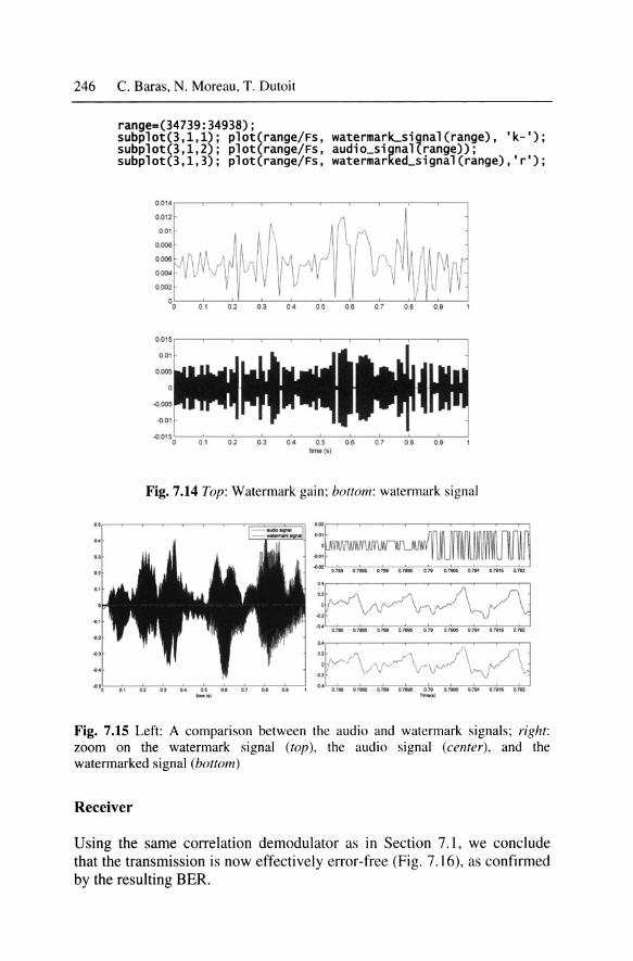
Plotting the gain for 1 second of signal, together with the resulting watermark signal and the audio signal, shows that the encoder has to make important adjustments as a function of the audio signal (Fig. 7.14 ).

subplot(2,1,1); plot((0:99)*N_samples/Fs, gain(1:100)); subplot(2,1,2); plot((O:Fs-1)/Fs, watermark_signal(1:Fs));

The watermark, though, is small compared to the audio signal (Fig. 7.15, left).

plot((O:Fs-1)/Fs, audio_signal(1:Fs)); hold on; plot((O:Fs-1)/Fs, watermark_signal(1:Fs), 'r-');

Plotting again a few samples of the watermark, audio, and watermarked signals shows that the watermarked signal sometimes differs significantly from the audio signal (Fig. 7 .15, right). This is confirmed by a listening test: the watermark is audible.


range=(34739:34938); subplot(3,1,1); plot(range/Fs, watermark_signal(range), 'k-'); subplot(3,1,2); plot(range/Fs, audio_signal(range)); subplot(3,1,3); plot(range/Fs, watermarked_signal(range), 'r');

~me lsi

Fig. 7.14 Top: Watermark gain; bottom: watermark signal

f~v/\-~~ · o.,. o.1e 0181 o,_ ue o.nca o.m o.ms o.JW -·

Fig. 7.15 Left: A comparison between the audio and watermark signals; right: zoom on the watermark signal (top), the audio signal (center), and the watermarked signal (bottom)

Receiver

Using the same correlation demodulator as in Section 7.1, we conclude that the transmission is now effectively error-free (Fig. 7.16), as confirmed by the resulting BER.


number_of_erroneous_bits= sum(bits -= received_bits) BER = number_of_erroneous_bits/total_number_of_bits

received_chars = reshape(received_bits(l:N_bits),N_bits/7, 7); received_message =char( bin2dec(num2str(received_chars)))'

number_of_erroneous_bits = 0 BER = 0

received_message = Audio watermarking: this message wi 77 be embedded in an audio signal, using spread spectrum modulation, and later retrieved from the modulated signal.

·:tl-:- ~ : : m : n 80 85 90 95 100 105 110 115 120 125 130

~~flb : : QlO : H ..Q.O 80 85 90 95 100 105 110 115 120 12.5 130

·Jl~' :m · o 80 85 90 95 100 106 110 11$ 120 1:2:5 130 ..... ""'""


7.2.3 Informed watermarking made inaudible

The informed watermarking system exposed in Section 7 .2.2 proves that prior knowledge of the audio signal can be efficiently used in the watermarking process; error-free transmission is reached, thanks to an adaptive embedding gain. However, the resulting watermark is audible, since no perceptual condition is imposed on the embedding gain. In this Section, we examine how psychoacoustics can be put to profit to ensure the inaudibility constraint. A psychoacoustic model is used, which provides a signal-dependent masking threshold used as an upper bound for the PSD of the watermark. The watermark gain is therefore replaced by an all-pole perceptual shaping filter, and the reception process is composed of a zero-forcing equalizer, followed by a linear-phase Wiener filter.


Emitter based on perceptual shaping filtering

The perceptual shaping filter is an auto regressive (all-pole) filter with 50 coefficients a i and gain bO. It is designed so that the PSD of the watermark (obtained by filtering the modul ated_s i gna l) equals the masking_threshold. The coefficients of the filter are obtained as in Chapter 1, via the Levinson algorithm. Both the masking threshold and the shaping filter have to be updated each time the statistical properties of the audio_signal change (here each N_windows=5l2 samples).

Let us first compute the masking threshold and apply the associated shaping filter to one audio frame (the lith frame, for instance; Fig. 7.17 left).

N_coef = 50; N_samples_PAM = 512; PAM_frame = (lO*N_samples_PAM+l lO*N_samples_PAM+N_samples_PAM);

plot(PAM_frame/Fs,audio_signal(PAM_frame) );

•r1·~:;-~ --;;7.--~----;;~-:;;.,-7.::---==:-------=' .,...[~

---------

Fig. 7.17 Left: Audio signal of frame #11; right: PSD of frame #II and the associated masking threshold and shaping filter response

Comparing the periodogram of the audio signal, the masking threshold, and the frequency response of the filter shows that the filter closely matches the masking threshold (Fig. 7.17 right). Even the absolute amplitude level of the filter is the same as that of the masking threshold. As a matter of fact, since the audio signal is normalized in [- 1 ,+ 1], its nominal PSD level is 0 dB.


MA TLAB functions involved:

• masking_threshold=psychoacoustical_model(audio_signal) returns the masking threshold deduced from a psychoacoustical analysis of the audio vector. This implementation is derived from the psychoacoustic model #1 used in MPEG-1 audio (see ISO/CEI norm 11172-3:1993 (F), pp. 122-128 or MATLAB function MPEG l_psycho_acoustic_modell.m from Chapter 3). It is based on the same principles as those used in the MPEG model, but it is further adapted here so as to make it robust to additive noise (which is a specific constraint of watermarking and is not found in MPEG).

• [bO,ai]=shaping_filter_design(desired_frequency_respons e_dB, N_coef) computes the coefficients of an auto-regressive filter

bO G(z) ----------------------------------------------

ai(l) + ai(2)z-1 + . . . + a i (N_coef) z-N_coef+l

(with ai(l)=l) from the modulus of its desi red_frequency_response (in dB) and the order N_coef. The coefficients are obtained as follows: if zero-mean and unity variance noise is provided at the input of the filter, the PSD of its output is given by desi red_frequency_response. Setting the coefficients so that this PSD best matches desi red_frequency_response is thus obtained by applying the Levinson algorithm to the autocorrelation coefficients of the output signal (computed itself from the IFFT of the desired_ frequency_response).

masking_threshold = ... psychoacoustical_model(audio_signal(PAMLframe));

shaping_filter_response = masking_threshold; [bO,ai]=shaping_filter_design(shaping_filter_response,N_coef);

%Plotting results. For details on how we use lpwelchl, see % the appendix of ASP_audio_cd.m, the companion script file of %chapter 2.

pwelch(audio_signal(PAM_frame),[],[],[],2); hold on; [H,W]=freqz(bO,ai ,256); stairs(W/pi,masking_threshold, 'k--'); plot(W/pi,20*loglO(abs(H)), 'r', 'linewidth' ,2); hold off;

Applying this perceptual shaping procedure to the whole watermark signal requires to process the audio signal block per block. Note that the filtering continuity from one block to another is ensured by the state


vector, which stores the final state of the filter at the end of one block and applies it as initial conditions for the next block.

state= zeros(N_coef, 1); for m = O:fix(N_bits*N_samples/N_samples_PAM)-1

end

PAM_frame = ... (m*N_samples_PAM+1:m*N_samples_PAM+N_samples_PAM);

% Shaping filter design maskin~_threshold = psychoacoustical_model( ...

audlo_signal(PAM_frame) ); shapin~_filter_response = masking_threshold; [bO, al]=shaping_filter_design(shaping_filter_response, ...

N_coef);

% Filtering stage [watermark_signal(PAM_frame,1), state] = ...

filter(bO, ai, modulated_signal(PAM_frame), state);

%Filtering the last, incomplete frame in lwatermark_signall PAM_frame = ...

(m*N_samples_PAM+N_samples_PAM+1:N_bits*N_samples); watermark_signal(PAM_frame,1) = ...


plot((O Fs-1)/Fs, audio_signal(1:Fs)); hold on plot((O Fs-1)/Fs, watermark_signal(1:Fs), 'r-');

J-~-- .. :v --.. /';: '/': ... / , .. :-.. J /,- '~ OtM 02'MIIo 0.,_ G_Ta ClJ'II O. :rel» 07t1 0:1'9U O.m .......

Fig. 7.18 Left: Audio signal and watermark signal; right: a few samples of the audio, watermark, and watermarked signals

The watermarked audio signal is still obtained by adding the audio signal and the watermark signal (Fig. 7.18 left). Plotting again few samples of the watermark, audio, and watermarked signals shows that the watermark signal has now been filtered (Fig. 7.18 right). As a result, the watermark is quite inaudible, as confirmed by a listening test. Its level, though, is similar to (if not higher than) that of the watermark signal in Section 7 .2.2.



range=(34739:34938); subplot(3,1,1); plot(range/Fs, watermark_signal(range), 'k'); subplot(3,1,2); plot(range/Fs, audio_signal(range)); subplot(3,1,3); plot(range/Fs, watermarked_signal(range),'r');

Receiver based on zero-forcing equalization and detection

The zero-forcing equalization aims at reversing the watermark perceptual shaping before extracting the embedded message. The shaping filter with frequency response shapi ng_fi lter _response is therefore recomputed from the audio watermarked_signal, since the original audio_signal is not available at the receiver. This process follows the same block processing as the watermark synthesis but involves a moving average filtering stage; filtering the watermarked_si gnal by the filter whose frequency response is the inverse of the shapi ng_fi l ter _response yields the filtered received signal denoted by equal i zed_si gna l.

Plotting the PSD of the equal i zed_si gna l shows its flat spectral envelope, hence its name (Fig. 7 .19).

state= zeros(N_coef, 1); for m = O:fix(N_bits*N_samples/N_samples_PAM)-1

end

PAM_frame = ... m*N_samples_PAM+1:m*N_samples_PAM+N_samples_PAM;

% shaping filter design, based the watermarked signal masking_threshold =

psychoacoustical_model(watermarked_signal(PAM_frame)); shapin~_filter_response = masking_threshold; [bO, al]=shaping_filter_design(shaping_filter_response, ...

N_coef);

% Filtering stage [equalized_signal(PAM_frame), state]= ...

filter(ai./b0,1,watermarked_signal(PAM_frame),state);

if m==10 % showing the frequency response of the equalizer and PSD %of the lequalized_si~nall, for frame 10.

pwelch(equalized_slgnal(PAM_frame),[],[],[],2); hold on;

end;

[H,W]=freqz(ai./b0,1,256); plot(W/pi,20*log10(abs(H)), 'r' ,'linewidth' ,2);

The equal i zed_si gna l is theoretically the sum of the original watermark (i.e., the modulated_signal, which has values in {-1,+1}) and the equalized_audio_signal, which is itself the original audio_signal filtered by the zero-forcing equalizer. In other words, from the receiver point of view, everything looks as if the watermark had been added to the equal i zed_audi o_si gnal rather than to the audi o_si gna l itself.


80

70

~~-t~1~~--~~~3--~0~~-0~.5~~~~8--~--~~~~ Nonnolizod Ftoquoney : L'(FI/2)

Fig. 7.19 Frequency response of the equalizer at frame #10 and PSD of the resulting equalized watermarked signal

Although the equa 1 i zed_audi o_s i gna 1 is not available to the receiver, it is interesting to compute it and compare it to the original audi o_si gna 1 (Fig. 7 .20, left). Note that the level of the equa 1 i zed_audi o_s i gna 1 is much higher than that of the original audi o_si gna 1, mostly because its HF content has been enhanced by the equalizer.

equalized_audio_signal = zeros(N_bits*N_samples, 1); state= zeros(N_coef, 1);

for m = O:fix(N_bits*N_samples/N_samples_PAM)-1

end

PAM_frame = ... m*N_samples_PAM+1:m*N_samples_PAM+N_samples_PAM;

% shaping filter design, based the watermarked signal masking_threshold = ...

psychoacoustical_model(watermarked_signal(PAM_frame)); shaping_filter_response = masking_threshold; [bO,ai]=shaping_filter_design(shaping_filter_response, ...

N_coef);

% Filtering stage [equalized_audio_signal(PAM_frame), state] = ...

filter(ai ./bO, 1, audio_signal(PAM_frame), state);

%Plotting 200 samples of the Jequalized_audio_signall, and % lmodulated_signall range=(34739:34938); subplot(2,1,1); plot(range/Fs, equalized_audio_signal(range)); subplot(2,1,2); plot(range/Fs, modulated_signal(range));


L...::-=---:~........::::---;;';:-;;;:::---;;:;;.--..:.,.;;:-. ..;->... I, ~ Mr.(\- (\f',f\1\ r!lt~, ·=~~f': ,) -vv\1 vvVW

_.0 .. , OJ' U OA 01 01 Ot 01 ... • ,..,......,...,_...,..,.,

Fig. 7.20 Left: Zoom on the equalized audio signal and on the modulated signal; right: corresponding PSDs

It is also possible to estimate the SNR by visual inspection of the PSDs of the equalized audio signal and the modulated signal (Fig. 7.20, right) or to compute it from the samples of these signals.

range=(34398:34938); ewelch(equalized_audio_signal(range),[],[],[],2); [h,w]=pwelch(modulated_signal (range),[],[],[] ,2); hold on; plot(w,10*log10(h),'--r ');

snr_equalized=10*log10(var(modulated_signal(range))/ . . . var(equalized_audio_signal(range)))

snr_equa Uzed = -19.0610

We can now proceed to the watermark extraction by applying the correlation demodulator to the equal i zed_si gna l and compute the BER. As expected, the obtained BER is quite high, since the SNR is low; the level of the equalized_audio_signal is high compared to that of the embedded modulated_signal (Fig. 7.20).

for m = O:N_bits-1

end

alpha(m+1) = (equalized_siynal(m*N_samples+l: ... m*N_samples+N_samples) * spread_waveform)/N_samples;

if alpha(m+1) <= 0 received_bits(m+1) = 0;

else received_bits(m+1) = 1;

end

% Plotting the input bits, alpha, and the received bits. range=(81:130); subplot(3, 1, 1); stairs(range, bits(range)); subplot(3,1,2); stairs(range, alpha(range)); subplot(3,1,3);


stairs(range, received_bits(range));

number_of_erroneous_bits= sum(bits -= received_bits) total_number_of_bits=N_bits BER = number_of_erroneous_bits/total_number_of_bits

received_chars = reshape(received_bits(1:N_bits),N_bits/7, 7); received_message =char( bin2dec(num2str(received_chars)))'

number_of_erroneous_bits = 30 tota l_number_of_bits = 1050 BER = 0.0286

received_message = udio watdrmarkyng:Oplks mussage will be embedded in e-Oaudik siwnql, }wi-g spread SpectruM(modul ·tion, and laterOretrieved from the modudated qiena 7.

Wiener filtering

The Wiener filtering stage aims at enhancing the SNR between the modu1ated_signal and the equalized_audio_signal. This is achieved here by filtering the equal i zed_si gna 1 by a symmetric (non causal) FIR filter with N_coef=50 coefficients. Its coefficients hi are computed so that the output of the filter (when fed with the equalized_signal) becomes maximally similar to the modulated_signal in the RMSE sense. They are the solution of the so-called Wiener-Hopf equations:

hi= equa1ized_signa1_cov_mat-1 * modulated_signal_autocor_vect where equalized_signal_cov_mat and modu1ated_signa1_autocor _vect are the covariance matrix of the equalized_signal and the autocorrelation vector of the modul ated_si gna l, respectively.

Since the modu 1 ated_si gna l is unknown from the receiver, its autocorrelation is estimated from an arbitrary modulated signal and can be computed once. To make it simple, we use our previously computed modu1ated_signal here. On the contrary, the covariance matrix of the equalized signal, and therefore the coefficients hi, has to be updated each time the properties of estimated_signa1 change, i.e., every N_samp1es_PAM=512 samples. Wiener filtering is then carried out by computing the covariance matrix of the equa 1 i zed_si gna l and the impulse response of the Wiener filter for each PAM frame.

modulated_signal_autocor_vect= ... xcorr(modulated_signal,N_coef,'biased');

state= zeros(2*N_coef, 1);

for m = O:fix(N_bits*N_samples/N_samples_PAM)-1 PAM_frame = ...

(m*N_samples_PAM+1:m*N_samples_PAM+N_samples_PAM);

end


%Estimating the covariance matrix of !equalized signal!, %as a Toeplitz matrix with first row given by the %autocorrelation vector of the signal. equalized_signal_autocor_vect= ...

xcorr(egualized_signal(PAM_frame),2*N_coef,'biased'); equalized_slgnal_cov_mat= ...

toeplitz(equalized_signal_autocor_vect(2*N_coef+1:end));

% Estimatin9 the impulse response of the wiener filter as % the solut1on of the wiener-Hopf equations. hi=equalized_signal_cov_mat\modulated_signal_autocor_vect;

% Filtering stage [wiener_output_signal(PAM_frame,1), state]= ...

filter(hi, 1, equalized_signal(PAM_frame), state); power = ...

norm(wiener_output_signal(PAM_frame))A2/N_samples_PAM; if (power -= 0)

wiener_output_signal(PAM_frame) = ...

end Wiener_output_signal(PAM_frame)/ sqrt(power);

% saving the wiener filter for frame #78 if m==78

end; hi_78=hi/sqrt(power);

% since the wiener filter is non-causal (with IN_coeffi=SO %coefficients for the non-causal part), the resulting %_1wiener_outpu~_signall is delayed with IN_coefl samples. Wlener_output_slgnal = ...

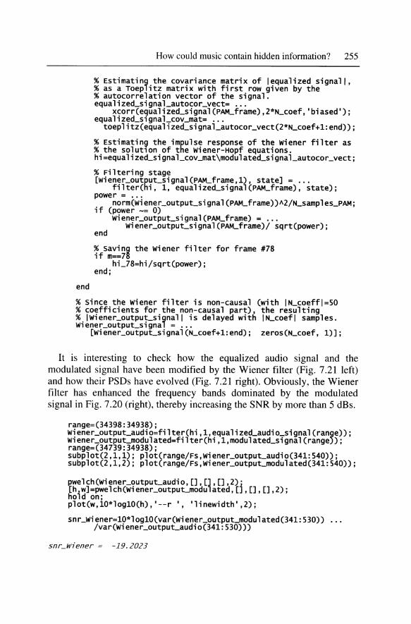
[Wiener_output_signal(N_coef+1:end); zeros(N_coef, 1)];

It is interesting to check how the equalized audio signal and the modulated signal have been modified by the Wiener filter (Fig. 7.21 left) and how their PSDs have evolved (Fig. 7.21 right). Obviously, the Wiener filter has enhanced the frequency bands dominated by the modulated signal in Fig. 7.20 (right), thereby increasing the SNR by more than 5 dBs.

range=(34398:34938); wiener_output_audio=filter(hi,1,equalized_audio_signal(range)); wiener_output_modulated=filter(hi,1,modulated_signal(range)); range=(34739:34938); subplot(2,1,1); plot(range/Fs,wiener_output_audio(341:540)); subplot(2,1,2); plot(range/Fs,wiener_output_modulated(341:540));

pwelch(wiener_output_audio,[],[],[],2); [h,w]=pwelch(wiener_output_modulated,[],[],[],2); hold on; plot(w,10*log10(h), '--r ', 'linewidth' ,2);

snr_wiener=10*log10(var(wiener_output_modulated(341:530)) /var(wiener_output_audio(341:530)))

snr_wiener = -19.2023


Fig. 7.21 Left: Zoom on the equalized audio signal and on the modulated signal passed through the Wiener filter; riKht: corresponding PSDs and frequency response of the Wiener filter

We can finally apply the correlation demodulator to the estimated modulated signal. The resulting BER is lower (Fig. 7.22), thanks to Wiener filtering ; a BER of the order of I 0-3 is reached, while the watermark is now inaudible.

for m = O:N_bits-1

end

alpha(m+l) = (Wiener_output_signal(m*N_samples+l: m*N_samples+N_samples)'*spread_waveform )/N_samples;

if alpha(m+l) <= 0 received_bits(m+l) = 0;

else received_bits(m+l) = 1;

end

number_of_erroneous_bits= sum(bits -= received_bits) total_number_of_bits=N_bits BER = number_of_erroneous_bits/total_number_of_bits

received_chars = reshape(received_bits(l:N_bits),N_bits/7, 7); received_message =char( bin2dec(num2str(received_chars)))'

number_of_erroneous_bits = 2 total_number_of_bits = 1050 BER = 0.0019

received_message =Audio watermarking: this message wi77$be embedded in an audio signal, using spread spectrum modulation , and later retrieved from the modulated signal .



Robustness to MPEG compression

We finally focus on the robustness of our system to MPEG compression. Using the MATLAB functions developed in Chapter 3, we can easily apply an mp3 coding/decoding operation to the audio watermarked signal, yielding the distorted watermarked audio signal compressed_watermarked_signal.

MA TLAB function involved:

• output_si gna l = codec_mp3 ( i nput_si gnal , Fs) returns the signal output_si gna l resulting from an mp3 coding/decoding operation of the input signal input_signal sampled at the Fs frequency sampling (see chapter 3).

compressed_watermarked_signal=mp3_codec(watermarked_signal,Fs);

We then pass the compressed signal through the zero-forcing equalizer and the Wiener filter, as before, and compute the resulting BER13 and received message.

BER = 0.1048

13 The corresponding MATLAB code can be found in the ASP_wat errnarking. rn file. We do not repeat it here.


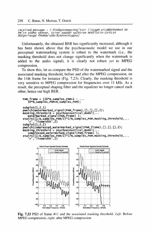
rece j ved_message = ) -%jm$gatemapcHng "txir } ! usagM whm&bo$embed 'de hN"cn yudho skenan, usjno ·sppdao sp}btrum mod57at7"o-(a!o£Lat %02gtd evgd fPoMda ''u0m/$uxetet4cggna}

Unfortunately, the obtained BER has significantly increased; although it has been shown above that the psychoacoustic model we use in our perceptual watermarking system is robust to the watermark (i.e., the masking threshold does not change significantly when the watermark is added to the audio signal), it is clearly not robust yet to MPEG compression.

To show this, let us compare the PSD of the watermarked signal and the associated masking threshold, before and after the MPEG compression, on the 11th frame for instance (Fig. 7.23). Clearly, the masking threshold is very sensitive to MPEG compression for frequencies over 11 kHz. As a result, the perceptual shaping filter and the equalizer no longer cancel each other, hence our high BER.

PAM_frame = (lO*N_samples_PAM+l: ... lO*N_samples_PAM+N_samples_PAM);

subplot(l,2,1) pwelch(watermarked_signal(PAM_frame),[],[],[],2); masking_threshold = psychoacoustical_model( ...

watermarked_signal(PAM_frame) ); stairs((l:N_samples_PAM/2)*2/N_samples_PAM,masking_threshold, ...

'r','linewidth',2) subplot(l,2,2) pwelch(compressed_watermarked_si9nal(PAM_frame),[],[],[],2); masking_threshold = psychoacoustlcal_model( ...

compressed_watermarked_signal(PAM_frame) ); stairs((l:N_samples_PAM/2)*2/N_samples_PAM,masking_threshold, ...

'r','linewidth' ,2)

·10

WOid1 PCHte< Spedral OoMi1y Estimole

-AudiollgM - Masl<logl!o-

1

"100o'---,o""=".2- o"' .• --="o.s:---:'o.-:-s ____, __ F...,uoncy of/(Fo/2)

Fig. 7.23 PSD of frame #11 and the associated masking threshold. Lefi: Before MPEG compression; right: after MPEG compression


7.2.4 Informed watermarking robust to MPEG compression

In order to improve the robustness of the system exposed in the previous section, the watermark information should obviously be spread in the [0 Hz, 11 kHz] frequency range of the audio signal. This can be achieved with a low-pass filter with cutoff frequency set to 11 kHz (Baras et al. 2006). As we shall see below, this filter will interfere with our watermarking system in three stages.

Designing the low-pass filter

First, we design a symmetric FIR low-pass filter with Fc=ll kHz cutoff frequency using the Parks-McClellan algorithm. Such a symmetric filter (Fig. 7.24, left) will have linear phase and therefore will not change the shape of the modulated signal more than required. We set the order of the filter to N_coef=50. Note that this filter is noncausal and introduces a N_coef /2-sample delay.

....

Fe = 11000; low_pass_filter = firpm(N_coef, [0 Fc-1000 Fc+1000 Fs/2]*2/Fs,

[1 1 1E-9 1E-9]); %low_pass_filter = ...

low_pass_filter/sqrt(sum(low_pass_filter)A2));

% Let us plot the impulse response of this filter. plot(low_pass_filter);

i~l : lg ..... ~-... :.------~, ---:o,s--+,---'

,.....,,., •to'

1·: , .... .....

· ~ ...........

........... - ·r-~ ~-

.o>!-, --=---=---=---=---=-----:! -. ' _.., ' . .... Fig. 7.24 Left: Impulse response of a symmetric FIR low-pass filter; right: its frequency response

It is easy to check that its frequency response matches our requirements (Fig. 7.24, right).

freqz(low_pass_filter,1,256);


Modifying the emitter

We first use this low-pass filter to create a spread sequence with spectral content restricted to the [0 Hz, II kHz] range. The modulated signal can then be designed as previously.

spread_waveform = ... filter(low_pass_filter,1,2*round(rand(N_samples+N_coef,1))-1);

% Getting rid of the transient spread_waveform = spread_waveform(N_coef+1:end); %Making sure the norm of the spread waveform is set to % sqrt(N_samples), as in the previous sections. spread_waveform = spread_waveform/ ...

sqrt(norm(spread_waveform).A2/N_samples);

for m = O:N_bits-1 modulated_signal(m*N_samples+1:m*N_samples+N_samples)

symbols(m+1)*spread_waveform; end

To prevent the shaping filter from amplifying the residual frequency component of the modulated signal over II kHz, the shapi ng_fi l ter _response, initially chosen to be equal to the masking threshold, is now designed to be equal to the masking threshold in the [0, 11 ]-kHz frequency band and to zero anywhere else.

state= zeros(N_coef, 1); N_cutoff = ceil(Fc/(Fs/2)*(N_samples_PAM/2));

for m = O:fix(N_bits*N_samples/N_samples_PAM)-1

end

PAM_frame = ... (m*N_samples_PAM+1:m*N_samples_PAM+N_samples_PAM);

% shaping filter design masking_threshold = ...

psychoacoustical_model( audio_signal(PAM_frame) ); shaping_filter_response = [masking_threshold(1:N_cutoff); ...

-100*ones(N_samples_PAM/2-N_cutoff, 1) ]; [bO,ai]=shaping_filter_design(shaping_filter_response,N_coef);

% Filtering stage [watermark_signal(PAM_frame), state] = ...


watermarked_signal = audio_signal + watermark_signal;

MPEG compression is then applied to the new watermarked_signal.

compressed_watermarked_signal=mp3_codec( watermarked_signal,Fs);


Modifying the receiver

Before starting the watermark extraction, the compressed_watermarked_si gna l is low-passed to avoid residual components over 11 kHz.

compressed_watermarked_signal = ••• filter(low_pass_filter, 1, [compressed_watermarked_signal;

zeros(N_coef/2, 1)]); %compensating tof the IN_coef/21 delay compressed_watermarked_signal = •••

compressed_watermarked_signal(N_coef/2+1:end);

Watermark extraction is finally obtained as in Section 7.2.3, except that the LP filter is again taken into account in the zero-forcing equalization. 14

The resulting BER is similar to the one we obtained with no MPEG compression; our watermarking system is thus now robust to MPEG compressiOn.

BER = 0.00095

received_message = ASdio watermarking: this message wi 11 be embedded in an audio signal, using spread spectrum modulation, and later retrieved from the modulated signa 1.

7.3 Going further

Readers interested in a more in-depth study of spread spectrum communications will find many details, as well as MA TLAB examples, in Proakis et al. (2004 ).

Several books on digital watermarking techniques are available. Cox et al. (2001) provides an intuitive approach, and many examples in C. Source code can also be found in Pan et al. (2004).

Also note that this chapter has mentioned only additive watermarking (yet only in the time domain), as opposed to the other main approach known as substitutive watermarking (Arnold et al. 2003). Moreover, additive watermarking can be performed in various domains, leading to various bit rate vs. distortion vs. robustness trade-offs (Cox et al. 2001): in the time domain, in the frequency domain, in the amplitude or phase domain (such as the one corresponding to the output of a modulated lapped transform, for robustness to small desynchronization; see Malvar and Florencio 2003), in the cepstral domain (often used in speech processing for its relation to the source/filter model; see Lee and Ho 2000), and in

14 The corresponding MATLAB code can be easily found in the ASP _watermarking. rn file. We do not repeat it here.


other parametric domains (such as the MPEG-compressed domain; see Siebenhaar et al. 2001). Last but not least, we have not examined synchronization problems here, which require special attention in the context of spread spectrum communications, since even a one-sample delay will have a disastrous effect on the resulting BER (Baras et al. 2006).

Security is one of the emerging challenges in watermarking (Furon et al. 2007). For more challenges, see, for instance, the BOWS challenges organized by the within European Network of Excellence ECRYPT (Bows2 2007).

7.4 Conclusion

Hiding bits of information in an audio stream is not as hard as one might think. It can be achieved by modulating the transmitted bits by a spread spectrum sequence and adding the resulting watermark signal to the audio stream. Making the watermark inaudible is a matter of dynamically shaping its spectrum so that it falls below the local masking threshold provided by a psychoacoustical model. Last but not least, ensuring that the system is robust to MPEG compression simply requires the addition of a low-pass filter in the spectrum-shaping stage.

Provided the receiver is able to invert the spectrum-shaping operation using the same psychoacoustical model as the emitter, and with the additional help of a Wiener filter to increase the SNR, a bit error rate of the order of 0.001 can be obtained.

References

Arnold M, Wolthusen S, Schmucker M (2003) Techniques and applications of digital water-marking and content protection. Artech House Publishers, Norwood,MA

Baras C, Moreau N, Dymarski P (2006) Controlling the inaudibility and maximizing the robustness in an audio annotation watermarking system. IEEE Transactions on Audio, Speech and Language Processing, 14-5:1772-1782

Bows2 (2007) Break our Watermarking system, 2nd edition [online] Available: http://bows2.gipsa-lab.inpg.fr [02/l/2008]

Chen B, Wornell G (2001) Quantization index modulation: A class of provably good methods for digital watermarking and information embedding. IEEE Transactions on Information Theory, 4 7: 1423-1443

Costa M (1983) Writing on dirty paper. IEEE Transactions on Information Theory, 29:439-441


Cox I, Miller M, Bloom J (2001) Digital watermarking: Principles and practice Morgan Kaufmann, San Francisco, CA

Cox I, Miller M, McKellips A (1999) Watermarking as communications with side information. Proceedings of the IEEE, 87-7:1127-1141

Craver SA, Wu M, Liu B (2001) What can we reasonably expect from watermarks? Proceedings of the IEEE Workshop on Applications of Signal Processing to Audio and Acoustics, New Paltz, NY, 223-226

Furon T, Cayre F, Fontaine C (2007) Watermarking security. In: Cvejic and Seppanen (eds) Digital Audio Watermarking Techniques and Technologies: Applications and Benchmarks. Information Science Reference, Hershey, PA, USA

Haykin S (1996) Adaptive filter theory, 3rd ed. Prentice-Hall, Upper Saddle River, NJ, USA

Jobs S (2007) Thoughts on music, [online] Available: http://www .apple.corn! hotnews/thoughtsonmusic/ [26/9/2007]

Larbi S, Jaidane M, Moreau N (2004). A new Wiener filtering based detection scheme for time domain perceptual audio watermarking. In IEEE International Conference on Acoustics, Speech and Signal Processing (ICASSP), Montreal, Canada, 5:949-952

Lee SK, Ho YS (2000) Digital audio watermarking in the cepstrum domain. IEEE Transactions on Consumer Electronics, 46-3: 744-750

LoboGuerrero A, Bas P, Lienard J (2003) Iterative informed audio data hiding scheme using optimal filter. In Proc. IEEE Int. Conf. on Communication Technology, Beijing, China, 1408-1411

Malvar H, Florencio D (2003) Improved spread spectrum: A new modulation technique for robust watermarking. IEEE Transactions on Signal Processing, 51-4:898-905

Massey JL (1994) Information theory aspects of spread-spectrum communications. IEEE Third International Symposium on Spread Spectrum Techniques and Applications (ISSSTA), 1:16-21

Pan JS, Huang HC, Jain LC (2004) Intelligent watermarking techniques (Innovative Intelligence). World Scientific Publishing Company, Singapore

Peterson RL, Ziemer RA, Borth DE (1995) Introduction to spread spectrum communications. Prentice Hall, Upper Saddle River, NJ, USA

Petitcolas FAP, Anderson RJ, Kuhn MG (1999) Information hiding - a survey. Proceedings IEEE, Special Issue on Protection of Multimedia Content, 87(7): 1062-1078

Proakis J (2001) Digital communications, 4th ed. McGraw-Hill, New York, USA Proakis JG, Salehi M, Bauch G (2004) Contemporary communication systems

using MA TLAB and SIMULINK. Brooks/Cole-Thomson Learning, Belmont, CA, USA

Shannon C ( 1958) Channel with side information at the transmitter. IBM Journal of Research and Development, 2:222-293

Siebenhaar F, Neubauer C, Herre J, Kulessa R (2001) New results on combined audio compression/watermarking. In 111th Convention of Audio Engineering Society (AES), New York, USA, preprint 5442

Date post:	08-Dec-2016
Category:	Documents
Upload:	ferran
View:	212 times
Download:	0 times

Applied Signal Processing || How could music contain hidden information?

Documents