j ourna l ho me page: www.elsev ier .com/ locate /asoc
ulti swarm bare bones particle swarm optimization withistribution adaption
eza Vafashoar ∗, Mohammad Reza Meybodioft Computing Laboratory, Computer Engineering and Information Technology Department, Amirkabir University of Technology, Tehran, Iran
r t i c l e i n f o
rticle history:eceived 9 November 2015eceived in revised form 30 April 2016ccepted 19 June 2016vailable online 23 June 2016
Bare bones PSO is a simple swarm optimization approach that uses a probability distribution like Gaussiandistribution in the position update rules. However, due to its nature, Bare bones PSO is highly proneto premature convergence and stagnation. The characteristics of the probability distribution functionsused in the update rule have a tense impact on the performance of the bare bones PSO. As a result,this paper investigates the use of different methods for estimating the probability distributions usedin the update rule. Four methods or strategies are developed that are using Gaussian or multivariateGaussian distributions. The choice of an appropriate updating strategy for each particle greatly dependson the characteristics of the fitness landscape that surrounds the swarm. To deal with issue, the cellularlearning automata model is incorporated with the proposed bare bones PSO, which is able to adaptivelylearn suitable updating strategies for the particles. Through the interactions among its elements andthe learning capabilities of its learning automata, cellular learning automata gradually learns to select
the best updating rules for the particles based on their surrounding fitness landscape. This paper also,investigates a new and simple method for adaptively refining the covariance matrices of multivariateGaussian distributions used in the proposed updating strategies. The proposed method is compared withsome other well-known particle swarm approaches. The results indicate the superiority of the proposedapproach in terms of the accuracy of the achieved results and the speed in finding appropriate solutions.
Particle swarm optimization (PSO) is a stochastic searchpproach inspired from the intelligent social behavior that existsmong some animals like bird and fish [1]. It consists of a swarmf particles flying in a search space for better solutions. The flighthich is guided by the velocity of particles resembles an itera-
ive search process. Particles adjust their velocities in this iterativeearch based on their own and social experiences. They can mem-rize their historical best visited locations and the historical bestisited location of the whole swarm.
Traditional PSO suffers from premature convergence and lowxploration ability, especially, when dealing with complex multiodal problems [2,3]. As a result, many researches proposed vari-
us approaches to remedy this problem. Parameter adaption [4–7],ybridization [8–10], incorporation of different updating, selection,utation strategies [11–13], topology variations [14–17], and inte-
gration of learning schemes [18–21] are some of the well-studiedmethods.
Studying the population dynamics and its convergence behav-ior [22], Kennedy suggested that the new positions of particles canbe obtained by sampling from an explicit probability distributionrather than using velocity information. In their work, the Gaussiandistribution is used for the acquisition of new positions, and itsparameters for a particular particle are exclusively defined by theinformers (particles utilized in its position updating) of the particle.The mean of the Gaussian distribution used in the position updaterule of a particular particle is defined as the average of the particle’sown historical best position and the swarm historical best posi-tion. Also, the distance of these two positions defines the standarddeviation of the distribution [23].
Bare bones PSO (BBPSO) still suffers from slow and prematureconvergence and stagnation. In the latter case, the swarm con-verges to non-optimal points [24–27]. Considering the definitionof updating distribution, the best particle of each iteration remains
unchanged during that iteration, which may result in stagnation.BBPSO with mutation and crossover operations (BBPSO-MC) han-dles this issue by employing the mutation strategy of differentialevolution algorithms in the update rule of the best particle [24].
ther mutation strategies like Gaussian or Cauchy are also exam-ned for improving bare bones PSO [25,28,29]. Krohling and Mendelroposed a jumping mechanism for avoiding local optima. Their
umping mechanism is based on the Gaussian or Cauchy noiseshich are added to the position of particles when they don’t
mprove for a period of time [28].Hybridizing bare bones PSO with other methods is also studied
y some researchers. Gao et al. introduced a bee colony algorithmhich produces candidate individuals in the onlooker phase based
n the update strategies of bare bones PSO. Because the particlesn bare bones PSO are attracted to the best individuals, the authorsonsidered this step as an improved exploitation phase [30].
Chen introduced a variant of bare bones PSO which uses aixture of two centers in the Gaussian distribution updating the
article positions. One of the centers is using local best positionsnd is considered to have exploration characteristics, while thether is based on the global best position and is used for betterxploitation around the best particle. At early iterations, explo-ation has a bigger weight which gradually decreases in the favorf exploitation [31,32].
Some other variants of bare bones PSO utilize heavy tail prob-bility distributions instead of Gaussian distribution for morexplorative behavior [25,29]. Li and Yao introduced a Cooperativearticle Swarms optimization method (CCPSO) for Large Scale Opti-ization. The population of CCPSO is divided into several swarms,
nd the swarms are updated cooperatively. The position of a par-icle at each step is updated similar to bare bones PSO; however,t uses different probability distributions for position sampling: aaussian distribution with its center at the best historical positionf the particle itself, and a Cauchy distribution whose center is at theocal best position. Either of the two distributions will be selected
ith a fixed probability for updating the particle position in eachimension. CCPSO, also, changes the number of swarms when thelobal best fitness value is not improving; this way, it can adaptivelydjust the number of swarms. BBPSO with scale matrix adapta-ion (SMA-BBPSO) uses multivariate t-distribution with adaptivecale matrices in its update rule. It employs a simple, yet effective,ethod for adapting the scale matrices associated with the parti-
les: the best position found by any particle in the neighborhoodf a particular particle is sampled in its associated scale matrix forhe next iteration.
This paper investigates the use of various probability models forpdating the positions of particles in BBPSO. Each model can ben-fit the search process depending on the shape of the landscapehere the particles reside. Some of the studied models involveultivariate Gaussian distributions for updating particle positions.ccordingly, a simple method for adapting the covariance matri-es of these Gaussian distributions will be introduced. To achieve aood performance, a strategy selection mechanism is needed. Thisechanism should select an appropriate updating strategy for each
article based on the properties of the particle’s surrounding land-cape. To achieve this objective, the swarms are embedded in aellular learning automata (CLA) [33–36], which adaptively learnshe best updating models for each particle. CLA is a hybrid math-matical model for many decentralized problems (decentralizedroblems can be considered as multiple systems where each systemas its own processing unit, and can make decisions according ton its own knowledge). It can be considered as a network of agentsith learning abilities. These agents have the ability to interact and
earn from each other through a set of CLA rules. CLA has been uti-ized in many scientific domains such as deployment and clusteringn wireless sensor networks [37,38], dynamic channel assignment
n cellular networks [39], evolutionary computing [40], and grapholoring [41].
The rest of the paper is organized as follows: Section 2 gives arief review on the involved concepts such as learning automata,
ft Computing 47 (2016) 534–552 535
cellular learning automata and particle swarm algorithm. Sec-tion 3 gives the detailed description of the proposed approach.Experimental results and comparison to other algorithms comesin Section 4, and finally Section 5 contains conclusions.
2. The involved concepts
This section provides a brief description of the concepts that areused in the paper. It starts with an introduction on particle swarmoptimization and Bare Bones PSO; then, reviews the basic conceptsof cellular learning automata.
2.1. PSO and related topics
Traditional PSO utilizes a population of particles called swarm.Each particle Xi in the swarm keeps information about its currentposition, its personal best visited position known as pbest, and itsflying velocity, respectively, in three D dimensional real valued vec-tors: xi = [xi1, xi2, . . ., xiD], pi = [pi1, pi2, . . ., piD], and vi = [vi1, vi2, . . .,viD]. All particles know the best position experienced by the wholeswarm known as gbest, which is also represented by a vector likepg = [pg1, pg2, . . ., pgD]. The search in a D dimensional space is an iter-ative process, during which the velocity and position of a particlelike Xi are updated according to the following equations:
where vid(k) is the dth dimension of the velocity vector of the parti-cle in step k; xid(k) and pid(k) are respectively the dth dimension ofits position and historical best position vectors; pgd(k) representsthe dth dimension of the historical best position of the whole swarmin step k; ω is the inertia weight, which was introduced to bringa balance between the exploration and exploitation characteristics[3]; c1and c2are acceleration constants that represent cognitive andsocial learning weights; and, finally, r1and r2are two random num-bers from the uniform distribution u(0, 1). After acquiring the newpositions of the particles, the historical best position of each par-ticle is updated; which may, also, affect the historical global bestposition of the swarm.
2.2. Bare bones particle swarm optimization
The observation of the motion of individual particles in the orig-inal PSO inspired the development of bare bones PSO. In traditionalPSO, the distribution of the positions visited by a single particleresembles the bell shaped curve of a Gaussian distribution. Accord-ingly, BBPSO uses Gaussian probability distribution to generate thenew position of a particle like Xi [23]:
xid(k + 1) = pid + plid2
+ N (0, 1) × |pid − plid| (2)
where N(0,1) denotes a random number taken from the normaldistribution with mean 0 and standard deviation 1. pl is the bestlocation, visited so far, in the neighborhood of the particle Xi, andpi is the personal best location of the particle itself.
2.3. Learning automaton
A variable structure learning automaton (LA) can be representedby a sextuple like {˚, �, �, A, G, P} [42]. where is a set of internalstates; � is a set of outputs or actions of the learning automaton;
� is a set of inputs or environmental responses; A is a learningalgorithm; G(.): → � is a function that maps the current state intothe current output; and P is a probability vector that determines theselection probability of an state at each stage. There is usually a one
5 ied Soft Computing 47 (2016) 534–552
tc
aesamLuisunt
p
p
pL
2
ufisictn
ftoan
2
balmtoic
cotblnpclc
LAjk
XjKLAi
k
Xik
LAlkXlk
A cellular learning automata with N cells, each cell resides a swarm of
Swarm k residing in cell k
The ith par�cle in the swarm k
The learning automaton ass igned to the ith par�cle of
swarm k
Three cells in the neighborhood of cell k
36 R. Vafashoar, M.R. Meybodi / Appl
o one correspondence between and �, as a results, the two termsan be used interchangeably.
The objective of a learning automaton is to identify the bestction which maximizes the expected received payoff from thenvironment [43]. To attain this goal, the learning automatonelects an action according to its action probability distribution,nd then applies this action to the environment. The environmenteasures the favorability of the received action, and responds the
A with a noisy reinforcement signal �. The learning automatonses this response to adjust its internal action probabilities via
ts learning algorithm. Consider the environmental response to aelected action like ai at step k be ∈ {0,1}, where 0 and 1 aresed as pleasant and unpleasant responses respectively. The inter-al action probability can be updated according to equation 3 whenhe response is pleasant and according to equation 4 when it is not.
j(k + 1) ={pj(k) + a(1 − pj(k)) if i = j
pj(k)(1 − a) if i /= j(3)
j(k + 1) =
⎧⎨⎩pj(k)(1 − b) if i = j
b
r − 1+ pj(k)(1 − b) if i /= j
(4)
In these two equations, a and b are called reward and penaltyarameters, respectively. For a = b the learning algorithm is calledR−P; when b � a, it is called LR�P; and when b is zero it is called LR−I
.4. Cellular automaton
A cellular automaton (CA) [44] is a collection of cells that aresually arranged in a regular form such as grid. Each cell has anite number of states, and in each time step, it is in one of thesetates. The cells evolve in time using a set of finite rules and localnteractions. The local interactions happen in the neighborhood ofells which is defined by the topology of the CA. At each time step,he set of rules defines the state of a cell based on the state of itseighboring cells at the previous time step.
A cellular automaton starts from some initial state, and evolvesor some time based on its rules, which results in complex pat-erns of behavior. The ability to produce different patterns usingnly local interactions and a set of simple rules has made cellularutomaton a popular tool for modeling complicated systems andatural phenomena.
.5. Cellular learning automata
Cellular learning automata (CLA) is a hybrid model which isased on cellular automata and learning automata theories. It is
collection of learning automata residing in the cells of a cellu-ar automaton. Each cell of the cellular automaton contains one or
ore learning automata, and the state of the cell is determined byhe states of its beholding learning automata. The neighboring cellsf a particular cell like c constitute the environment of the learn-ng automata residing in c. The interactions among the cells areontrolled using a set of rules, termed as CLA rules.
A CLA starts from some initial state, which is the state of all of itsells. During each step, the learning automata select actions basedn their internal probability distributions. The actions are appliedo the environment of the corresponding learning automata, andased on the CLA rules, reinforcement signals are returned to the
earning automata. Then, each learning automaton adjusts its inter-al probability distribution according to its received signals. This
rocedure continues for period of some steps until a terminationondition is satisfied. Mathematically, a CLA can be defined as fol-ows. A d-dimensional CLA with a single learning automaton in eachell is a structure A =
(Zd, N, �, A, F
)where:
M par�cles, and a group of M learning automata
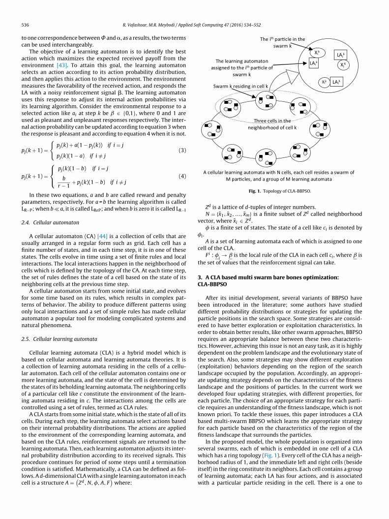
Fig. 1. Topology of CLA-BBPSO.
Zd is a lattice of d-tuples of integer numbers.N = {x1, x2, ..., xm} is a finite subset of Zd called neighborhood
vector, where xi ∈ Zd.� is a finite set of states. The state of a cell like ci is denoted by
�i.A is a set of learning automata each of which is assigned to one
cell of the CLA.Fi : �
i→ is the local rule of the CLA in each cell ci, where is
the set of values that the reinforcement signal can take.
3. A CLA based multi swarm bare bones optimization:CLA-BBPSO
After its initial development, several variants of BBPSO havebeen introduced in the literature; some authors have studieddifferent probability distributions or strategies for updating theparticle positions in the search space. Some strategies are consid-ered to have better exploration or exploitation characteristics. Inorder to obtain better results, like other swarm approaches, BBPSOrequires an appropriate balance between these two characteris-tics. However, achieving this issue is not an easy task, as it is highlydependent on the problem landscape and the evolutionary state ofthe search. Also, some strategies may show different exploration(exploitation) behaviors depending on the region of the searchlandscape occupied by the population. Accordingly, an appropri-ate updating strategy depends on the characteristics of the fitnesslandscape and the positions of particles. In the current work wedeveloped four updating strategies, with different properties, foreach particle. The choice of an appropriate strategy for each parti-cle requires an understanding of the fitness landscape, which is notknown priori. To tackle these issues, this paper introduces a CLAbased multi-swarm BBPSO which learns the appropriate strategyfor each particle based on the characteristics of the region of thefitness landscape that surrounds the particles.
In the proposed model, the whole population is organized intoseveral swarms, each of which is embedded in one cell of a CLAwhich has a ring topology (Fig. 1). Every cell of the CLA has a neigh-
borhood radius of 1, and the immediate left and right cells (besideitself) in the ring constitute its neighbors. Each cell contains a groupof learning automata; each LA has four actions, and is associatedwith a particular particle residing in the cell. There is a one to
Table 1A brief definition of notations used in the paper.
Notation Description Notation Description
Xki
the ith particle in the kth swarm xki(t) the current position of Xk
iat time t
pki(t) personal best position of Xk
iat time t pkg (t) the global best position of the kth swarm
pkid
(t) the value of pki(t) in the dth dimension �(k,j) the jth neighbor of the kth cell (or swarm). j = 0, 1, 2
respectively refer to the kth cell (swarm), its left cell(swarm), and right cell (swarm).
pkiI(t) The value of pk
i(t) in dimensions presented by I, where Ik
i(t) the partition of dimensions which is used by Xk
iat time t.
oaaTtaCAdTt
3
ooeoppmcsrso
I ⊆ {1, 2, ..., D}gk(t) the index of the best particle in the kth swarm
M The size of each swarm
ne correspondence between the actions of a learning automatonnd the updating strategies of its associated particle. The learningutomata govern the strategy application of their related particles.he proposed model uses multiple swarms rather than a single oneo maintain a natural diversity in the population. Also, the inter-ctions that exist among the neighboring cells and swarms enableLA to learn suitable strategies (actions) for its beholding particles.
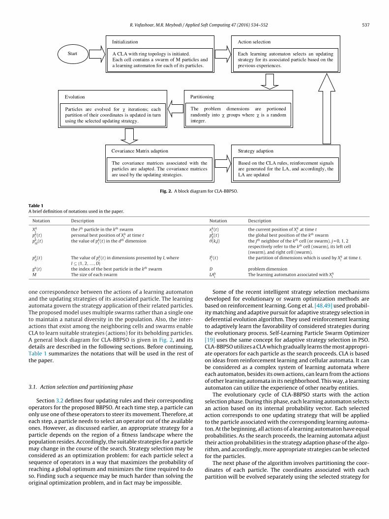
general block diagram for CLA-BBPSO is given in Fig. 2, and itsetails are described in the following sections. Before continuing,able 1 summarizes the notations that will be used in the rest ofhe paper.
.1. Action selection and partitioning phase
Section 3.2 defines four updating rules and their correspondingperators for the proposed BBPSO. At each time step, a particle cannly use one of these operators to steer its movement. Therefore, atach step, a particle needs to select an operator out of the availablenes. However, as discussed earlier, an appropriate strategy for aarticle depends on the region of a fitness landscape where theopulation resides. Accordingly, the suitable strategies for a particleay change in the course of the search. Strategy selection may be
onsidered as an optimization problem: for each particle select a
equence of operators in a way that maximizes the probability ofeaching a global optimum and minimizes the time required to doo. Finding such a sequence may be much harder than solving theriginal optimization problem, and in fact may be impossible.
D problem dimensionLAki
The learning automaton associated with Xki
Some of the recent intelligent strategy selection mechanismsdeveloped for evolutionary or swarm optimization methods arebased on reinforcement learning. Gong et al. [48,49] used probabil-ity matching and adaptive pursuit for adaptive strategy selection indeferential evolution algorithm. They used reinforcement learningto adaptively learn the favorability of considered strategies duringthe evolutionary process. Self-Learning Particle Swarm Optimizer[19] uses the same concept for adaptive strategy selection in PSO.CLA-BBPSO utilizes a CLA which gradually learns the most appropri-ate operators for each particle as the search proceeds. CLA is basedon ideas from reinforcement learning and cellular automata. It canbe considered as a complex system of learning automata whereeach automaton, besides its own actions, can learn from the actionsof other learning automata in its neighborhood. This way, a learningautomaton can utilize the experience of other nearby entities.
The evolutionary cycle of CLA-BBPSO starts with the actionselection phase. During this phase, each learning automaton selectsan action based on its internal probability vector. Each selectedaction corresponds to one updating strategy that will be appliedto the particle associated with the corresponding learning automa-ton. At the beginning, all actions of a learning automaton have equalprobabilities. As the search proceeds, the learning automata adjusttheir action probabilities in the strategy adaption phase of the algo-rithm, and accordingly, more appropriate strategies can be selectedfor the particles.
The next phase of the algorithm involves partitioning the coor-dinates of each particle. The coordinates associated with eachpartition will be evolved separately using the selected strategy for
5 ied So
titc(ocs
p(sdi
oe
3
ucsatO
x)|if (
(t −
x
ab(aTito
b
|anastd
ri
38 R. Vafashoar, M.R. Meybodi / Appl
he particle. Accordingly, if the coordinates of a particle are dividednto � partitions, the particle will be updated for � times duringhe next evolutionary phase. As we intend to evolve all of the parti-les for the same number of times during each evolutionary phaseto attain a fair comparison of their performances), the coordinatesf each particle are partitioned in a same manner as other parti-les. To achieve this objective, first, D is partitioned into � randomummands (D, problem dimensionality, is an integer number):
D =∑�
i=1ai
where : ai = 2k, k = {1, 2, ..., MAXP}; i<� and a� ∈ Z+ − {1}
(5)
Here MAXP is a parameter controlling the maximum size of eachartition. As the summands are generated randomly, their number�) may vary in different partitioning phases. Using these orderedummands, the coordinates of each particle are partitioned ran-omly into � groups where the size of the ith group equals to the
th summand (ai):⋃�j=1I
ki(t + j) = {1, 2, ..., D}
where :
|Iki(t + j)| = ai
(6)
Here Iki(t + j) is the jth partition of coordinates for the ith particle
f swarm k, which will be used during the (t + j)th iteration of thevolution phase.
.2. Updating rules of CLA-BBPSO
Considering different aspects of problems, we define fourpdating strategies for CLA-BBPSO. The strategies have differentharacteristics that enhance various aspects of the search. The firsttrategy is the classical update rule of the BBPSO algorithm. It uses
Gaussian sampling which is based on the information present inhe neighborhood of a particle.perator A, Gaussian operator:
If d ∈ Iki(t):
kid(t) =
{pkid
(t − 1) + pkgd
(t − 1) /2 + N 0, 1 × |pkgd
(t − 1) − pkid
(t − 1
pkid
(t − 1) + p�(k,r)gd
(t − 1) /2 + N 0, 1 × |p�(k,r)gd
(t − 1) − pkid
If d /∈ Iki(t):
kid(t) = pkid(t − 1)
This operator alters the dth dimension of a particle using random number taken from Gaussian probability distri-ution. For particles other than a swarm’s best particle,
pkid
(t − 1) + pkgd
(t − 1))/2 and |pk
gd(t − 1) − pk
id(t − 1)| will be used
s the mean and standard deviation of the Gaussian distribution.herefore, non-global best particles in a swarm use inter swarmnformation to guide their movements. These particles aim for bet-er exploitation of the found promising locations in the swarm. Inrder to explore the best locations out of the swarm, the global
est particle of the swarm uses(pkid
(t − 1) + p�(k,r)gd
(t − 1))/2 and
p�(k,r)gd
(t − 1) − pkid
(t − 1)| as the parameters of the Gaussian oper-tor where r ∈ {1, 2} is a random number identifying a randomeighboring swarm. In order to prevent drastic random changesnd to utilize previously learned information, a particle retainsome of its historical best position’s information in its new posi-ion and updates the others as stated previously. I(t) identifies the
imensions of a particle to be updated during the iteration.
When the new position in dimension d falls out of the searchange, it is re-generated (in dimension d) using the operator A untilt sticks inside the search range.
ft Computing 47 (2016) 534–552
i, k) /= (gk(t − 1), k)
1)|otherwise(7)
Operator B, multivariate Gaussian operator with covariancematrix �:
xki (t) ={N pk
i(t − 1) + pkg /2,
∑ki if (i, k) /= (gk(t − 1), k)
N pki(t − 1) + p�(k,r)
g (t − 1) /2,∑k
i otherwise(8)
Operator A changes the value of each coordinate in the positionvector independent from the values of other coordinates. How-ever, it is useful to consider the existent interdependencies amongthe coordinates of the problem landscape. Covariance is a mea-sure of how much two random variables change together, and amultivariate Gaussian distribution utilizing a covariance matrix canrepresent the dependencies among the dimensions of a landscape.Motivated from this idea, some evolutionary algorithms managethe correlations between coordinates through covariance matri-ces [45–47]. Operator B changes the position of a particle basedon the multivariate Gaussian distribution with mean � and covari-ance matrix ˙. When a particle is not the best particle of its swarm,(pki
+ pkg)/2 will be used as the mean of its associated distribution;
otherwise,(pki
+ p�(k,r)g
)/2 will be used (similar to operator A). The
covariance matrix associated with a particular particle is adaptedduring the search (as will be discussed later).
Re-generating a vector for handling out of range search maybe computationally inefficient; therefore, the method presented in[19] will be used when operator B results in out of range positions:
xkid(t) =
⎧⎪⎨⎪⎩xkid
(t) if xkid
(t) ∈ [xd,min, xd,max]
u pkid
(t − 1), xd,max if xkid
(t) > xd,max
u xd,min, pkid
(t − 1) if xkid
(t) < xd,min
(9)
where u(a,b) generates a random number between a and b.Operator C, multivariate Gaussian operator with partial covari-ance matrix:
Operator B resamples all of the coordinates of a personal best
position to generate a new position; therefore, some promisinginformation may be lost. In order to relax this issue, Operator Cis defined to affect only some coordinates. Let I = Iik(t) ⊆{1, 2, 3,. . .,
D} represent these coordinates, and let∑k
iI be the projection of∑k
iinto these coordinates; then, operator C defines a new position as:
If d ∈ Iki(t):
xkiI(t) ={N pk
iI(t − 1) + pkgI /2,
∑kiI if (i, k) /= (gk(t − 1), k)
N pkiI(t − 1) + p�(k,r)
gI (t − 1) /2,∑k
iI otherwise(10)
If d /∈ Iki(t):
xkid(t) = pkid(t − 1)
Operator C handles the out of range search in the same way asOperator B.Operator D, multivariate Gaussian operator with partial samplecovariance matrix:
Estimation of distribution algorithms use explicit distributionmodels like multivariate Gaussian distribution for sampling new
points. Then, employing the promising newly generated points,they refine their probabilistic models. Inspiring from this idea,operator D uses the sample covariance matrix and the sample meanin the Multivariate Gaussian distribution (Let I = Iik(t)):
ied So
x
x
wd
�
�
)
3
wulmTegcp
p
wwusm
C
w
sar
vaAu∑
tib
R. Vafashoar, M.R. Meybodi / Appl
If d ∈ Iki(t):
kiI(t) = N
(�kiI, �
kiI
)(11)
If d /∈ Iki(t):
kid(t) = pkid(t − 1)
here the sample mean and the sample covariance matrices areefined as follows:
kiI(t) =
⎧⎪⎨⎪⎩
1M
∑M
j=1pkjI(t − 1) if (i, k) /= (gk(t − 1), k)
13
∑2
j=0p�(k,j)gI (t − 1)otherwise
(12)
ˆ kiI
=
⎧⎪⎨⎪⎩
1M
∑M
j=1
(pkjI(t − 1) − �k
iI(t))(pkjI(t − 1) − �k
iI(t))Tif (i, k) /= (gk(t − 1), k)
13
∑2
j=0
(p�(k,j)gI
(t − 1) − �kiI(t))(p�(k,j)gI
(t − 1) − �kiI(t))Totherwise
(13
.3. Covariance matrix adaption
Each particle has a covariance matrix incorporated with it,hich is evolved alongside the particle itself. Operators B and Cse this covariance matrix in order to direct the particle in the
andscape. Hansen and his colleagues proposed some covarianceatrix adaptation mechanisms for evolution strategies [45–47].
hey introduced rank-1 and rank-� update rules to ensure a reliablestimator. At each generation, the information from the previousenerations is used to refine the covariance matrix. Rank 1 uses theoncept of evolutionary path which is the whole path taken by theopulation over a number of generations, and is defined as follows:
(g+1)c = (1 − cc)p
(g)c +
√cc(2 − cc)�eff
m(g+1) − m(g)
�(g)(14)
here cc is the backward time horizon, and pc (0) = 0; m(g) is theeighted mean of the best selected samples at generation g. rank-�pdate rule uses an estimation for the distribution of the selectedteps along with the previous information about the covarianceatrix:
(g+1) = (1 − ccov)C(g) + ccov∑
wiyi(g+1)yi
(g+1)T (15)
here yi(g+1) =
(x(g+1)i
− m(g))/�(g), and wi is the weight of the
elected sample; � represents the step size, which is also updatedt each generation. Using these rules together, the overall updateule can be like the following:
C(g+1) = (1 − ccov)C(g) + ccov
(1 − 1
�cov
)∑wiyi
(g+1)yi(g+1)T
+ ccov�cov
pc(g+1)pc
(g+1)T (16)
BBPSO with scale matrix adaptation (SMA-BBPSO) uses multi-ariate t-distribution to update the position of particles. It employs
simple method for adapting the scale matrix of the t-distribution.t each iteration, the scale matrix related to the kth particle ispdated using the following equation:
k= (1 − ˇ)
∑k
+ ˇnknTk (17)
ˇ is the learning rate controlling the portion of the scale matrixo be inherited from the past experience, and nk is the best positionn the neighborhood of the kth particle. The idea is simple, and isased on sampling the best found positions into the scale matrix.
ft Computing 47 (2016) 534–552 539
Employing the previous concepts, CLA-BBPSO uses two mech-anisms to adapt the covariance matrix of each particle. First, itutilizes the evolution direction of the particle. This concept resem-bles the concept of evolution path. The evolution direction () ofparticle Xk
iwill be defined as follows:
ki (t) =(pki (t) − pki (t
′)) (pki (t) − pki (t
′))T
(18)
where t and t’, respectively, represent the current iteration num-ber and the iteration number during the previous covariance matrixadaption phase. Accordingly, pk
i(t) is the current personal best loca-
tion of the particle Xki, and pk
i(t′) is its personal best position at
the time of previous covariance matrix adaption phase. Evolutiondirection samples the last improvement of a particle. Like Eq. (17),we also sample the best nearby position into the covariance matri-ces. However, considering the sample covariance matrix definition,which is given in Eq. (13), one can interpret the sample covarianceas the average dependencies of the data samples with respect totheir mean. In this interpretation if we only consider the depen-dency of the best point, we can obtain:
nki(t) − m nk
i(t) − m
T
where : nki(t) = arg min f (p) , p ∈
{plj(t)|l ∈ �(k, s), s = 0, 1, 2
}− pk
i(t)
(19)
Here nki(t) is the best position in the neighborhood of the par-
ticle Xki. m is the mean of the distribution, and as it is unknown,
it should somehow be estimated. We, simply, will use pki(t) as the
mean of the distribution. In this way, the best nearby dependencywith respect to pk
i(t) will be sampled into the covariance matrix.
Using this interpretation, if Xki
happens to be the best particle inits own neighborhood, then the above equation evaluates to zero.Therefore, we defined nk
i(t) as the best nearby position other than
pki(t) itself. Equation 19 is very similar to Equation (17); though, in
17, m is missing which is similar to assuming a zero value mean.As we shall see in the experimental section, assuming m = 0 may betroublesome on shifted test functions that have their optimum in alocation other than the origin. Based on the aforementioned ideas,the overall equation for covariance matrix adaption in CLA-BBPSOis:∑k
i(t) = (1 − ˇ)
∑k
i(t′) + ˇSki (20)
where:
Ski
= 12
(pki (t) − pki (t
′)) (pki (t) − pki (t
′))T
+12
(nki (t) − pki (t)
) (nki (t) − pki (t)
)T (21)
3.4. Strategy adaption
After action selection phase, each particle is evolved for a periodof several iterations. Afterwards, the strategy adaption phase isapplied to adjust the action probabilities in the favor of the mostpromising ones. The favorability of a selected action for a learningautomaton is measured based on the comparison of its outcomewith the outcomes of the selected actions in the adjacent cells. Theoutcome of an action will be measured according to the amount ofimprovement in the fitness value of the associated particle, whichis defined as follows:
ki = 1
f (pk(t))
(f (pki (t
′)) − f (pki (t)))
(22)
i
where t is the current iteration number, and t’ is the iteration num-ber in the previous strategy adaption phase. Accordingly, f (pk
i(t))
and f (pki(t′)) represent the fitness of the particle Xk
i, respectively, in
5 ied So
tmf
ˇ
Bt4Oiwoetw
cf
4
modaswRcintcsawmctsnxnco
pstiabmmpomtan
40 R. Vafashoar, M.R. Meybodi / Appl
he current and previous adaption phases. Based on the improve-ent values of the particles in its adjacent cells, the reinforce signal
or a learning automaton like LAki
is obtained as follows:
ki ={
0 if ki> median
{ lj|l = �(k, h), h = 1, 2
}1otherwise
(23)
Here median returns the statistical median of its argument set.ased on the received reinforcement signal, each learning automa-on updates its internal action probabilities using equations 3 or. This definition for reinforcement signals has some advantages.n average, the promising actions of about half of the learn-
ng automata are rewarded, hence, these actions can be selectedith higher probabilities next times. The selected actions of the
ther half are panelized; therefore, these learning automata willxplore other actions (other operators) with higher probabilitieshan before. This way, we can ensure that each operator alwaysould have a chance of selection.
After strategy adaption phase, the algorithm continues a newycle starting with the action selection phase. A general pseudocodeor the proposed model is given in Fig. 3.
. Experimental study
This section demonstrates the effectiveness of the proposedethod through experimental study and comparison. The behavior
f the method is studied on a set of benchmark functions that areefined in Table 2. These functions possess various characteristics;s a result, they can exhibit different properties of the stochasticearch methods. The set contains 2 unimodal functions f8 and f9,hile the others are multimodal. Although, the two dimensionalosenbrock’s function (f11) is unimodal, its higher dimensionalases are considered to be multimodal. In higher dimensional cases,t possesses two optima with the global one residing inside a long,arrow, and parabolic shaped valley with a flat bottom. The func-ions can also be categorized according to the separability of theiroordinates. Separable functions, including functions f1–f9, can beolved using independent searches in each of their coordinates. As
result, some mutation or crossover based simple search methods,hich are somehow simulating coordinate independent search, canislead evaluations. In order to alleviate this problem, Table 2, also,
ontains a set of inseparable functions, problems f10–f16. Some ofhese inseparable problems are the rotated versions of their originaleparable cases. By rotating a function one can make its coordi-ates inseparable. To rotate a function like f(x), the original vector
is left multiplied with an orthogonal matrix M: y = M × x, and theew generated vector y is used to calculate the fitness of its asso-iated individual. We use the Salomon’s method to generate therthogonal matrices [51].
Many stochastic search approaches start with random initialopulations, and using some stochastic operators, explore theearch space. The result of some operators tends to have a biasoward the mean point of the population. In the case of randomnitialization and symmetric problem landscapes, this mean pointpproaches the center of the search space. Looking at Table 2, it cane seen that except f1 all of the test problems have their global opti-um at the center of the search space. These issues may result inisleading performance evaluations as in the case of the two recent
ublished works [25,52]. Hence, we employed the shifted versionf the given functions, where f(x − �) is used instead of f(x) to deter-
ine the fitness. We set � to [0.2U1, 0.2U2, . . ., 0.2UD] where Ui is
he upper boundary of the ith coordinate, and applied this shift toll of the functions except f1, which already has its optimum pointear the boundaries.
ft Computing 47 (2016) 534–552
4.1. Compared PSO algorithms
CLA-BBPSO is compared with a group of PSO algorithms whoseconfigurations are summarized in Table 3. The results of all algo-rithms are taken from 30 independent runs. Each run of analgorithm on a benchmark function is terminated after 105 fitnessfunction evaluations on 30-D functions, and 3 × 10⁵ fitness functionevaluations on 50-D functions.
SMA-BBPSO is a variant of Bare Bones PSO which uses a multi-variate t-distribution for sampling the new positions of particles. It,also, adapts the scale matrix of each particle by sampling the bestposition in its neighborhood with the maximum likelihood. PS2OSRresembles CLA-BBPSO in that both are utilizing multiple swarms ofparticles. In PS2OSR, a particle is attracted to three informers: his-torical best positions of itself and its own swarm along with thebest historical position in its neighboring swarms. Comprehensivelearning particle swarm optimizer (CLPSO) is mainly developed fordealing with complex multimodal functions. Each coordinate ofa particle learns comprehensively from the corresponding coor-dinate of another particle or the corresponding coordinate of thehistorical best position of itself until it fails to improve for a periodof time. CLPSO updating procedure results in a diversified popula-tion, which ensures its high exploration capability; however, thediversified population results in a low convergence rate. In fullyinformed PSO (FIPS), all the neighbors contribute to the velocityadjustment. The sum of acceleration coefficients is considered to bea constant value, which is equally divided between the accelerationcoefficients. Frankenstein PSO (FPSO) starts with a fully connectedtopology, and gradually decreases the connectivity of the particles.Adaptive PSO (APSO) uses the population distribution and fitnessinformation to adjust the inertia weight and acceleration coeffi-cients. Starling PSO is based on the collective response of starlings.When the global best position of the swarm doesn’t improve for aperiod, the velocity and position of particles are adjusted based ontheir neighboring particles. The way to handle the out of rang searchis not discussed clearly in the original paper for Starling PSO. Themethod of handling search boundaries may have a critical impacton the performance of the PSO approaches. For a fair comparison,we implemented the boundary handling methods of CLA-BBPSO forStarling PSO. In summary, Starling PSO is implemented with maxvelocity of 0.2 of the search ranges, and Eq. (9) is used for handlingthe search boundaries. The same equation, also, will be used forSMA-BBPSO.
4.2. A note on the max partition size
One advantage of multi swarm approaches is their locality,which means that each swarm operates utilizing only local infor-mation. However, if we have to partition the coordinates of everyparticle in a same way, as discussed previously, this locality willbe violated. This partitioning can be done locally if we set MAXP to1. Furthermore when MAXP = 1, the search process can get betterinformation on how much two coordinates of a particle belongingto a same group are correlating with each other. Therefore, fromthe next sections the value of 1 will be used for MAXP. Though,this section investigates the effect of different values of MAXP onthe performance of the proposed method. Fig. 4a to 4e show theeffect of different values of MAXP on a group of benchmarks selectedfrom Table 2. As the results suggest, the algorithm performed bet-ter with MAXP = 1 on most of the tested problems. The definitionof rotated hyper-ellipsoid function (f10) suggests that to refine acandidate solution all of its coordinates somehow should change
together as they are highly correlated. For this function, chang-ing a value in one coordinate of a fine candidate solution generallyworsens the candidate’s fitness. Also, as we will see in Section 4.6,the learning mechanism tends to select mostly operator B for f10.
Fig. 4. The statistical results on f3(a), f5(b), f10(c), f11(d), and f12(e) for different values of MAXP. The results are obtained from 30 independent runs.
function Search range Opt value Required precision
f1 = 418.9829 × D +N∑i=1
(−xi sin
(√|xi|))
[−500,500]D 0 0.001
f2 =N∑i=1
(−x2
i− 10 cos(2xi) + 10
)[−5.12,5.12]D 0 0.001
f3(X) = f2(Z),
zi =
{xi if |xi| <
12
round(2xi)2
if |xi| ≥ 12
[−5.12,5.12]D 0 0.001
f4 = −20 exp
⎡⎣−0.2
√√√√ 1N
N∑i=1
x2i
⎤⎦
− exp
[1N
N∑i=1
cos(2xi)
]+ 20 + exp(1)
[−32,32]D 0 0.001
f5 = 14000
N∑i=1
x2i
−N∏i=1
cos
(xi√i
)+ 1 [−600,600]D 0 0.00001
f6 =
N
⎧⎨⎩
10sin2(y1) + (yN − 1)2+N−1∑i=1
(yi − 1)2[
1 + 10 sin2(yi+1)]⎫⎬⎭
+N∑i=1
u(xi, 10, 100, 4), yi = 1 + 14
(xi + 1)
u(xi, a, k, m) ={k(xi − 1)mxi > a0 − a ≤ xi ≤ ak(−xi − a)mxi < −a
[−50,50]D 0 0.001
f7 = 0.1
⎧⎪⎨⎪⎩
sin2(3x1) + (xN − 1)2[
1 + sin2(2xN )]
+N−1∑i=1
(xi − 1)2[
1 + sin2(3xi+1)]
⎫⎪⎬⎪⎭
+N∑i=1
u(xi, 10, 100, 4)
[−50,50]D 0 0.001
f8 =N∑i=1
x2i
[−100,100]D 0 0.001
f9 =N∑i=1
|xi| +N∏i=1
|xi| [−10,10]D 0 0.001
f10 =N∑i=1
[i∑j=1
xj
]2
[−100,100]D 0 0.001
f11 =N−1∑j=1
[100(xj+1 − x2
j)2 + (xj − 1)2
][−100,100]D 0 30
f12: f2(y), y = M*x [−5.12,5.12]D 0 50f13: f5(y), y = M*x [−600,600]D 0 0.00001f14: f4(y), y = M*x [−32,32]D 0 0.001f15: f3(y), y = M*x [−5.12,5.12]D 0 50f16: f1(y), y = M*x [−500,500]D 0 3000
Table 3Parameter settings for the compared PSO algorithms.
Method parameter settings
PS2OSR [17] c = 1.3667, � = 0.729CLPSO [38] c = 1.49445, w ∈ [0.4, 0.9]FIPS [11] ϕ = 4.1, � = 0.7298FPSO [14] ϕ = 4.0, w ∈ [0.4, 0.9]APSO [6] 1.5 < c1, c2 < 2.5 and c1 + c2 < 4, w ∈ [0.4, 0.9]SMA-BBPSO[25] Max M = 5, neighborhood size = 3, Swarm size = 30Starling PSO[52] Swarm Size = 50; Stagnant limit = 2; Max Num = 14; c1 = c2 = 2; wmax = 0.4; wmin = 0.2;
ied So
Oaasar
4
si1sstwip
ooructarc
ifbob
4
mtfisaatbsrbe
epwTt
rc(opwfh
R. Vafashoar, M.R. Meybodi / Appl
perator B changes the coordinates of a particle all together whichpproves the latter idea. As operator B somehow plays the rule of
large MAXP, the tendency of functions like f10 for larger partitionizes becomes clearer if we disable this operator. Finally, as oper-tor B plays the rule of a large MAXP, MAXP = 1 shows to be a lessestriction.
.3. Parameter settings for CLAB-BPSO
The proposed CLA-based BBPSO involves some parameters thathould be adjusted. The population size is set to 40 as suggestedn the PSO literature. This population can be divided into 20, 13,0, 8, . . . swarms according to the number of particles in eachwarm. However, using few swarms with large swarm sizes maypoil the multi swarm features of the algorithm. Therefore, we keephe number of swarms large enough. We have tested CLA-BBPSOith the number of swarms equal to 20, 13 (the population size
s 39 in this case) and 10, and used 10 in the experiments of thisaper. The other topologies yield very similar results.
The other parameters are the reward and punishment factorsf the learning automata. For these two parameters a vast rangef values can be used, and their effect is deeply investigated in theelated literature. As a result, based on our previous experience, wesed a = 0.2 and b = 0.02. The only remaining parameter is � whichontrols the portion of the covariance matrix to be inherited fromhe past experiences (equation 20). The effect of this parameter on
set of benchmarks is studied in this section. Fig. 5a to 5e show theesults of the algorithm on a set of benchmark problems when �hanges in the range [0.1 0.9].
For two problems f1 and f2, different values for � have a littlempact on the achieved final results. On f10, the algorithm per-ormed better when � is near 0.4. On f11, � < 0.5 yields, somehow,etter final results. The algorithm has, somehow, better behaviorn f12 when � ∈ [0.3, 0.8]. From these observations � = 0.4 seems toe an appropriate choice.
.4. Experimental results on 30-D test problems
The first test of this section examines the speed of the comparedethods in finding a global optimum or nearing an acceptable solu-
ion. The study is performed by obtaining the average number oftness function evolutions required to reach the specified preci-ions given in Table 2. A run of an algorithm on a benchmark isllowed to continue until the maximum number of fitness evalu-tions. If a run of an algorithm can’t reach the required precision,hen the run will be considered as unsuccessful. The average num-er of successful runs on a benchmark (which will be called theuccess rate of the method on the benchmark) can represent theobustness of an algorithm. This section compares the methodsased on their success rates and the average number of fitnessvolutions on their successful runs.
The precisions that are given in Table 2 are defined in a way tonsure the detection of global optima; however, none of the com-ared methods can reach the global optimum of some benchmarksith a high precision in the allowable number of fitness evolutions.
herefore, some larger precisions are considered for these functionso make the comparisons sensible.
The comparison results are given in Table 4. CLA-BBPSO is supe-ior to the other peer algorithms according to the success rateriteria; it achieved the specified threshold on almost all of the runsexcept for one run on f16) on every tested benchmark function. Allf the other peer PSO methods have failed to reach the specified
recisions on many runs. All of the runs of APSO on f1, f2, and f10ere unsuccessful. The same is true for CLPSO on f3, f10, f13, and
14. FIPS has zero success rates on four benchmark functions. FPSOas zero success rates on 10 benchmarks; while, the success rate of
ft Computing 47 (2016) 534–552 543
PS2OSR is zero on 4 benchmarks. From another point of view, APSOhas a success rate lower than one on 13 benchmarks; CLPSO haslower success rate on 10 benchmarks; FIPS has lower success rateon 9 benchmarks; the success rate of FPSO is lower than 1 on 13benchmarks; and finally, PS2OSR is unsuccessful on some runs of 10tested benchmark functions. From these observations, the robust-ness and superiority of the purposed method in comparison to theother peer methods can easily be concluded.
Although CLAB-BPSO isn’t the fastest compared method inreaching the specified precisions, its speed in nearing the specifiedthresholds is very competitive to the fastest ones. Some of the com-pared methods possess higher convergence speeds, which resultedin their insufficient explorative ability and premature convergence.
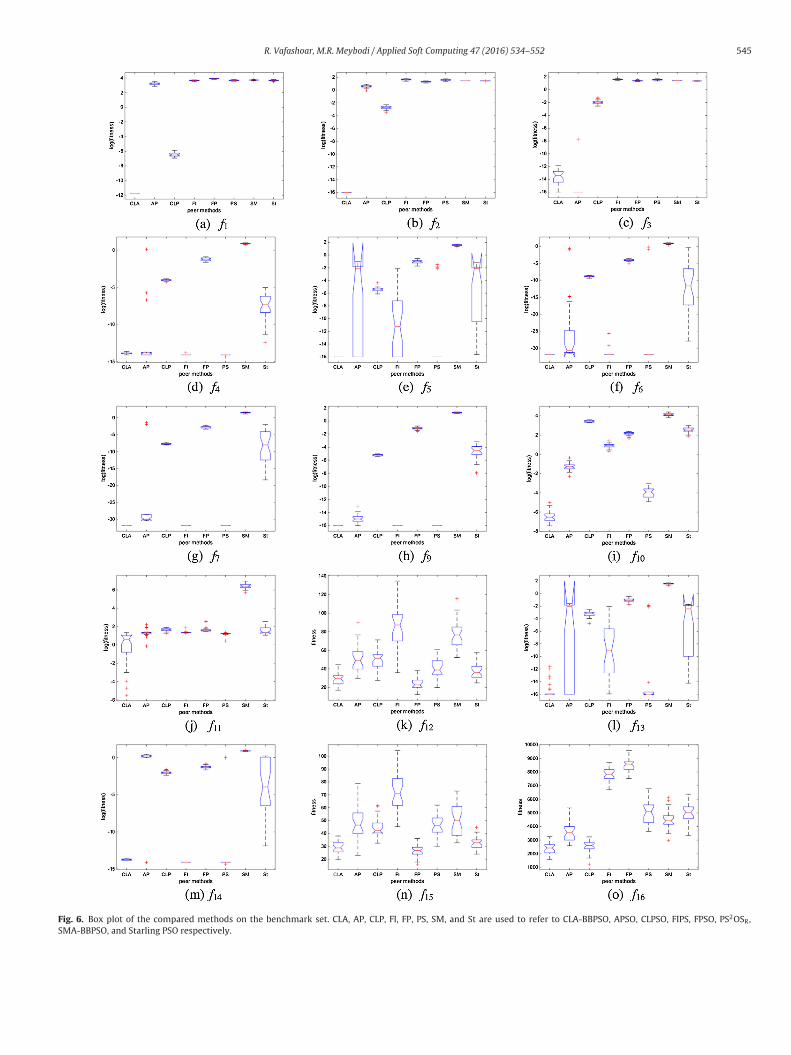
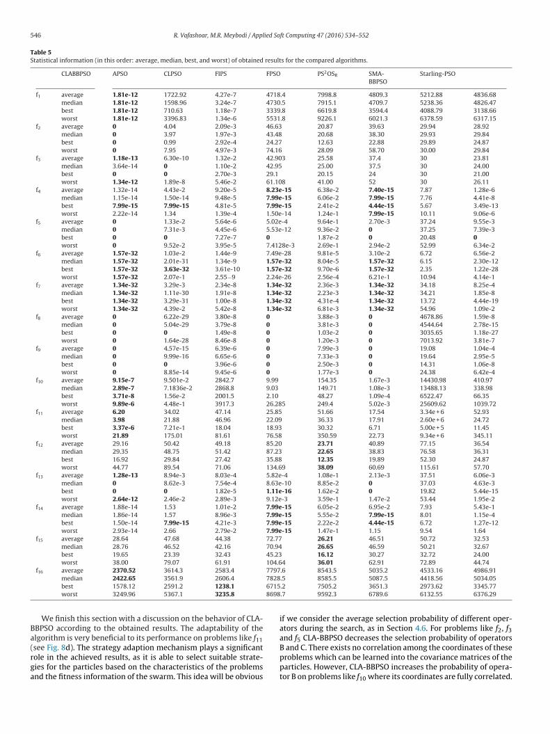
The next experiment is conducted to compare the accuracy ofthe compared algorithms. Each method is tested on each of thebenchmark functions for 30 runs, and the statistical information ofthe achieved final results on the benchmark functions is used forcomparison. Table 5 gives these statistical information in terms ofaverage, median, best, and worst on each benchmark, the distribu-tion of the final results are illustrated in Fig. 6. Also, the Wilcoxonrank sum test for a confidence level of 95% [50] has been utilizedto compare the methods from statistical point (Table 6). Wilcoxontest is a nonparametric alternative to the paired t-test [50], and isbased on the null hypothesis that the two compared algorithmsare statistically equivalent. For each test ‘+’ is used if the proposedapproach is better than a compared algorithm, ‘−’ for the oppositecase, and ‘=’ if the two algorithms are statistically indistinguishable.
The first note on the results of Table 5 is about Starling PSO.The obtained results of Starling PSO are much weaker than theones which could be obtained on the un-shifted versions of the testfunctions. We believe that using equations 3 and 4 (in [52]) leads tothis difference, and the orientation change introduced by these twoequations results in a bias toward the center of the search space.Also, the results of SMA-BBPSO in Table 5 are much weaker thanthe ones reported in [25]. We believe that this difference is causedbecause of two reasons:
1. Eq. (14) in [25], which is used to update the covariance matrix,resembles equation 19 when the mean is considered to be zero.It samples the dependency of the best point into the covariancematrix with respect to m = 0. However, symmetric test functionshave their optimum point at the center of the search space;therefore, Eq. (14) (in [25]) learns the dependency of the bestsample with respect to the problem solution (which should beconsidered unknown).
2. The second reason may be due to the fact that we used equa-tion 9 for boundary handling in SMA-BBPSO. However, as itisn’t mentioned how boundaries are handled in SMA-BBPSO, weutilized the boundary handling mechanisms of CLA-BBPSO intoSMA-BBPSO.
Observing Table 5, it is clear that the proposed method has thehighest accuracy among all of the compared methods on most ofthe tested problems. CLA-BBPSO has the best average on 12 bench-marks; while, its average results on the other four benchmarks arevery near to the best ones. The obtained results of the purposedmethod are very distinctive from all of the other peer methods onthe benchmarks: f1, f2, f10, and f11. Also, only 3 algorithms werecapable of finding the global optimum of f3, with CLA-BBPSO hav-ing the highest average. Although CLA-BBPSO doesn’t possess the
best average results on f4 and f14, its obtained results are very com-petitive to the best obtained ones. Also, CLA-BBPSO has the secondbest results on f12 and f16, and its achieved results are very near tothose of FPSO (the best method on these benchmarks).
Fig. 5. The statistical results on f1(a), f2(b), f10(c), f11(d), f12(e) when � changes in the range [0.1, 0.9].
Table 4Average number of evaluations needed to reach the specified accuracy for successful runs along with the average success rates inside parenthesis.
Considering the results of Wilcoxon test we can conclude the
tatistical superiority of the proposed algorithm to both APSO andLPSO. CLA-BBPSO is statistically superior to CLPSO on all of theested problems. Comparing CLA-BBPSO to APSO, CLA-BBPSO is sta-istically inferior to APSO on f3, is statistically indistinguishable
on f4, and is statistically superior on the rest of tested problems.
In Comparison to PS2OSR, CLA-BBPSO is better on 9 benchmarkproblems, is statistically indistinguishable on 4 benchmarks, andis statistically worst only in 2 cases.
Fig. 6. Box plot of the compared methods on the benchmark set. CLA, AP, CLP, FI, FP, PS, SM, and St are used to refer to CLA-BBPSO, APSO, CLPSO, FIPS, FPSO, PS2OSR,SMA-BBPSO, and Starling PSO respectively.
Table 5Statistical information (in this order: average, median, best, and worst) of obtained results for the compared algorithms.
CLABBPSO APSO CLPSO FIPS FPSO PS2OSR SMA-BBPSO
Starling-PSO
f1 averagemedianbestworst
1.81e-121.81e-121.81e-121.81e-12
1722.921598.96710.633396.83
4.27e-73.24e-71.18e-71.34e-6
4718.44730.53339.85531.8
7998.87915.16619.89226.1
4809.34709.73594.46021.3
5212.885238.364088.796378.59
4836.684826.473138.666317.15
f2 averagemedianbestworst
0000
4.043.970.997.95
2.09e-31.97e-32.92e-44.97e-3
46.6343.4824.2774.16
20.8720.6812.6328.09
39.6338.3022.8858.70
29.9429.9329.8930.00
28.9229.8424.8729.84
f3 averagemedianbestworst
1.18e-133.64e-1401.34e-12
6.30e-10001.89e-8
1.32e-21.10e-22.70e-35.46e-2
42.90342.9529.161.108
25.5825.0020.1541.00
37.437.52452
30303030
23.8124.0021.0026.11
f4 averagemedianbestworst
1.32e-141.15e-147.99e-152.22e-14
4.43e-21.50e-147.99e-151.34
9.20e-59.48e-54.81e-51.39e-4
8.23e-157.99e-157.99e-151.50e-14
6.38e-26.06e-22.41e-21.24e-1
7.40e-157.99e-154.44e-157.99e-15
7.877.765.6710.11
1.28e-64.41e-83.49e-139.06e-6
f5 averagemedianbestworst
0000
1.33e-27.31e-309.52e-2
5.64e-64.45e-67.27e-73.95e-5
5.02e-45.53e-1207.4128e-3
9.64e-19.36e-21.87e-22.69e-1
2.70e-3002.94e-2
37.2437.2520.4852.99
9.55e-37.39e-306.34e-2
f6 averagemedianbestworst
1.57e-321.57e-321.57e-321.57e-32
1.03e-22.01e-313.63e-322.07e-1
1.44e-91.34e-93.61e-102.55−9
7.49e-281.57e-321.57e-322.24e-26
9.81e-58.04e-59.70e-62.56e-4
3.10e-21.57e-321.57e-326.21e-1
6.726.152.3510.94
6.56e-22.30e-121.22e-284.14e-1
f7 averagemedianbestworst
1.34e-321.34e-321.34e-321.34e-32
3.29e-31.11e-303.29e-314.39e-2
2.34e-81.91e-81.00e-85.42e-8
1.34e-321.34e-321.34e-321.34e-32
2.36e-32.23e-34.31e-46.81e-3
1.34e-321.34e-321.34e-321.34e-32
34.1834.2113.7254.96
8.25e-41.85e-84.44e-191.09e-2
f8 averagemedianbestworst
0000
6.22e-295.04e-2901.64e-28
3.80e-83.79e-81.49e-88.46e-8
0000
3.88e-33.81e-31.03e-21.20e-3
0000
4678.864544.643035.657013.92
1.59e-82.78e-151.18e-273.81e-7
f9 averagemedianbestworst
0000
4.57e-159.99e-1608.85e-14
6.39e-66.65e-63.96e-69.45e-6
0000
7.99e-37.33e-32.50e-31.77e-3
0000
19.0819.6414.3124.38
1.04e-42.95e-51.06e-86.42e-4
f10 averagemedianbestworst
9.15e-72.89e-73.71e-89.89e-6
9.501e-27.1836e-21.56e-24.48e-1
2842.72868.82001.53917.3
9.999.032.1026.285
154.35149.7148.27249.4
1.67e-31.08e-31.09e-45.02e-3
14430.9813488.136522.4725609.62
410.97338.9866.351039.72
f11 averagemedianbestworst
6.203.983.37e-621.89
34.0221.887.21e-1175.01
47.1446.9618.0481.61
25.8522.0918.9376.58
51.6636.3330.32350.59
17.5417.916.7122.73
3.34e + 62.60e + 65.00e + 59.34e + 6
52.9324.7211.45345.11
f12 averagemedianbestworst
29.1629.3516.9244.77
50.4248.7529.8489.54
49.1851.4227.4271.06
85.2087.2335.88134.69
23.7122.6512.3538.09
40.8938.8319.8960.69
77.1576.5852.30115.61
36.5436.3124.8757.70
f13 averagemedianbestworst
1.28e-13002.64e-12
8.94e-38.62e-302.46e-2
8.03e-47.54e-41.82e-52.89e-3
5.82e-48.63e-101.11e-169.12e-3
1.08e-18.85e-21.62e-23.59e-1
2.13e-3001.47e-2
37.5137.0319.8253.44
6.06e-34.63e-35.44e-151.95e-2
f14 averagemedianbestworst
1.88e-141.86e-141.50e-142.93e-14
1.531.577.99e-152.66
1.01e-28.96e-34.21e-32.79e-2
7.99e-157.99e-157.99e-157.99e-15
6.05e-25.55e-22.22e-21.47e-1
6.95e-27.99e-154.44e-151.15
7.938.016.729.54
5.43e-11.15e-41.27e-121.64
f15 averagemedianbestworst
28.6428.7619.6538.00
47.6846.5223.3979.07
44.3842.1632.4361.91
72.7770.9445.23104.64
26.2126.6516.1236.01
46.5146.5930.2762.91
50.7250.2132.7272.89
32.5332.6724.0044.74
f16 average 2370.52 3614.3 2583.4 7797.6782867158698
8543.5 5035.2 4533.16 4986.91
Ba(rga
medianbestworst
2422.651578.123249.96
3561.92591.25367.1
2606.41238.13235.8
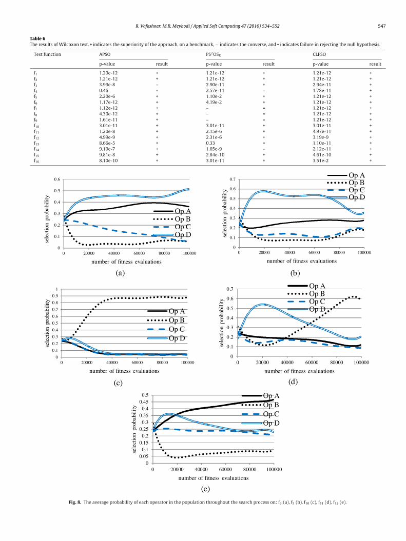
We finish this section with a discussion on the behavior of CLA-BPSO according to the obtained results. The adaptability of thelgorithm is very beneficial to its performance on problems like f11
see Fig. 8d). The strategy adaption mechanism plays a significantole in the achieved results, as it is able to select suitable strate-ies for the particles based on the characteristics of the problemsnd the fitness information of the swarm. This idea will be obvious
.5
.2
.7
8585.57505.29592.3
5087.53651.36789.6
4418.562973.626132.55
5034.053345.776376.29
if we consider the average selection probability of different oper-ators during the search, as in Section 4.6. For problems like f2, f3and f5 CLA-BBPSO decreases the selection probability of operators
B and C. There exists no correlation among the coordinates of theseproblems which can be learned into the covariance matrices of theparticles. However, CLA-BBPSO increases the probability of opera-tor B on problems like f10 where its coordinates are fully correlated.
Table 6The results of Wilcoxon test. + indicates the superiority of the approach, on a benchmark, − indicates the converse, and = indicates failure in rejecting the null hypothesis.
Fig. 8. The average probability of each operator in the population throughout the search process on: f3 (a), f5 (b), f10 (c), f11 (d), f12 (e).
5 ied So
Aaohaoliet
alstooatoitcgfand
4
Stmrlm
taboiitoebwasd
4
mitfiAapt
48 R. Vafashoar, M.R. Meybodi / Appl
lso, the algorithm balances the exploration and exploitation char-cteristics of the search through operator selection; as, dependingn the fitness dynamics, some of the proposed operators tend toave more exploration or exploitation characteristics. Considering
problem like f1, which has its optimum point near the boundariesf the search space, CLA-BBPSO is capable of diversifying the popu-ation to discover the boundaries of the search space, which CLPSOs also capable of. It also can achieve a proper balance betweenxploration and exploitation, which enables the proposed methodo achieve more accurate results than CLPSO on this function.
As CLA-BBPSO seems to be more explorative than the otherpproaches, its convergence speed may be low on some problemsike f8 and f9 (Table 5). However, the developed operators may haveome impact in this matter. Other operators would be developedhat can acquire more knowledge of the fitness landscape insteadf operators A, and D. These operators are based on simple Gaussianr multivariate Gaussian distributions, and utilize little informationbout the landscape properties or the past experiences of the par-icles. Finally, FPSO obtained a little better results than CLA-BBPSOn f12 and f15 (also consider FIPS uses a higher connectivity, andts results are weaker than the other peer methods on these func-ions). FPSO uses a dynamic topology where it starts with a fullyonnected population and gradually decreases its connectivity. Ineneral, the topology of the population can greatly affect the per-ormance of the swarm approaches. Like different strategies, theppropriate topology for the population greatly depends on the fit-ess landscape. Accordingly, CLA-BBPSO can be extended to utilizeynamic topologies to achieve better performances.
.5. Experimental results on 50-D test problems
This section conducts the experiments of the second part ofection 4.4 on the 50-D test problems where the accuracy ofhe methods on the given benchmarks is compared after a maxi-
um number of fitness evaluations. Table 7 provides the statisticalesults of the compared algorithms on each of the benchmark prob-ems. Also, Fig. 7 provides the distribution of the solutions of each
ethod on the benchmark set.The experimental results on 50-D functions are much similar to
heir 30-D cases. CLABBPSO obtained the best average on almostll of the tested functions except f12, where it achieved the secondest average fitness just behind FPSO. The achieved average resultsf none of the peer methods are better than CLA-BBPSO (exceptn one case), and CLA-BBPSO is superior to each of them in somenstances. In terms of average obtained results, CLA-BBPSO is betterhan APSO on 13 benchmark problems and is somehow equivalentn the other 3; it is better than CLPSO on all of the benchmarksxcept f1; in comparison with FPSO, CLA-BBPSO is better on 15enchmarks and is a little worst on only f12; comparing CLABBPSOith FIPS and PS2SR, its better on respectively 10 and 14 functions
nd is equivalent on the reminder. From these observations, theuperiority of CLA-BBPSO over other peer methods can be easilyeducted.
.6. A study on the learning capabilities of CLA-BBPSO
This section studies the effect of the proposed action selectionechanism on the performance of the algorithm, and illustrates
ts functioning. Fig. 8 shows how the operator probabilities varyhroughout the algorithm’s iterations on a group of benchmarksrom Table 2. Each figure represents the average operator probabil-ty in the population over the spent number of fitness evaluations.
s it can be seen from the figures, each test problem requires oper-tors with different characteristics. For separable problems therobabilities of operators B and C reduce over time, and get lowerhan the probabilities of operators A and D. This may be due to the
ft Computing 47 (2016) 534–552
fact that no dependency exists among their coordinates which canbe learned over time. However, the type of dependencies among thecoordinates of hyper-ellipsoid function completely fits with opera-tor B. Therefore, the probability of operator B is increased over time.For the other two test functions, the probabilities change accord-ing to the state of the population at different stages of the searchprocess.
To demonstrate that the algorithm actually has learning capa-bilities, it is statistically compared with its pure chance version(actions are selected with equal probability all the time). For thispurpose, Wilcoxon test is used to demonstrate the statistical dif-ference of the two versions. The results of this test are providedin Table 8. From Table 8, CLA-BBPSO is statistically superior to thepure chance version on 11 benchmarks, and is statistically indis-tinguishable on the reminder. In addition, on the latter instances,CLA-BBPSO was better than its pure chance version in terms of theconvergence speed (which would have been clear if we comparedthem using convergence curves).
4.7. Time complexity of the proposed approach
This section investigates the time complexity of the proposedapproach. As the evolutionary phase of the proposed method isanalogous to other simple evolutionary or swarm optimizationmethods, this section analyzes the overhead of other phases of theproposed approach on the evolutionary phase. There are 4 phasesto consider: action selection, partitioning, covariance matrix adap-tion, and strategy adaption. Before continuing, let us assume thatthe population size is n, i.e. N × M = n, also, the problem dimen-sionality is D. Action selection simply selects an action for eachlearning automaton based on its probability vector. As the numberof actions is a small constant (4), this phase can be performed in alinear time with respect to n, i.e. o(n). Action selection is repeatedonce for every D/2 iterations of the evolution phase, so its overheadto each iteration of the evolution phase is o(2n/D) = o(n/D). As weare using partitions of size two, the partitioning phase can be per-formed independently for each particle by randomly permutatingits coordinates, which can be performed in o(D); hence, its overallcontribution to each iteration of the evolution phase is o(n). Covari-ance matrix adaptation phase includes finding the best particle inthe neighborhood of each particle, and simple matrix operations.The first part can be performed efficiently in o(n) for all particles,and the second one in o(D2) for each particle. So, the overhead ofthis phase on each iteration is o(n/D + nD) = o(nD). The overhead ofstrategy adaption phase can be similarly computed, which is o(n/D).The used updating operators, except operator B are simple and havea low time complexity. While generating samples from multivari-ate Gaussian distribution using operator B is time consuming, thisoperator may be selected fewer times than the others.
To conclude this section, we provided the average run times ofeach peer method on the benchmark functions given Table 2. Therun time of an algorithm greatly depends on the efficiency of theimplementation, used data structures, and the running platform;however, it may give an insight on the complexity of the proposedmethod. Looking at Table 9, it is obvious that the proposed methodis slower than the other peer methods on many instances, whichwas predictable. Algorithms like FPSO do not have much overheadas CLA-BBPSO, and each of their generations involves only a fewsimple operations. However, the proposed method is not muchslower. Besides, on time consuming functions like f6 and f7 theruntime ratio of different methods approaches to 1.
There remains two more points to discuss. First, as the pro-
posed updating strategies have different time complexities, andthe method may select the most complex one more than the oth-ers (or vice versa), its runtime on some problems may be lowerthan some simpler ones. Second, APSO has a very long run time on
Fig. 7. Box plot of compared methods on the benchmark set. CLA, AP, CLP, FI, FP, PS, SM, and St are used to denote CLA-BBPSO, APSO, CLPSO, FIPS, FPSO, PS2OSR, SMA-BBPSO,and Starling PSO respectively.
Table 7Statistical information (in this order: average, median, best, and worst) of obtained results for the compared algorithms.
CLAMS APSO CLPSO FIPS FPSO PS2OSR
f1 averagemedianbestworst
2.08e-112.18e-111.81e-112.18e-11
2990.62732.8710.636761.8
2.18e-112.18e-112.18e-112.18e-11
8614.38621.46704.710624
14003141221219615167
8723.38737.86830.311311
f2 averagemedianbestworst
0000
2.421.980.995.96
7.49e-24.47e-23.23e-35.42e-1
93.7293.1958.23112.11
42.7941.1230.5655.64
80.4677.6061.68116.41
f3 averagemedianbestworst
0000
0000
3.974.062.346.61
88.4589.3167.07114.09
44.6744.2433.1755.04
92.4192.8555.32135.50
f4 averagemedianbestworst
1.93e-142.22e-141.51e-142.22e-14
7.33e-52.22e-141.50e-142.19e-3
1.85e-81.80e-81.32e-82.91e-8
1.42e-141.50e-147.99e-151.50e-14
9.03e-28.25e-23.76e-22.47e-1
8.52e-27.99e-157.99e-151.37
f5 averagemedianbestworst
0000
1.49e-28.62e-301.06e-1
8.45e-112.16e-115.20e-131.11e-9
1.47e-3003.67e-2
1.76e-11.54e-14.21e-23.77e-1
2.21e-3001.23e-2
f6 averagemedianbestworst
9.42e-339.42e-339.42e-339.42e-33
8.29e-31.61e-302.94e-316.22e-2
3.33e-163.10e-161.05e-167.04e-16
1.65e-29.42e-339.42e-332.48e-1
2.51e-33.42e-41.19e-46.30e-2
7.47e-29.42e-339.42e-336.86e-1
f7 averagemedianbestworst
1.34e-321.34e-321.34e-321.34e-32
6.22e-31.49e-276.63e-304.39e-2
3.66e-153.26e-151.55e-158.15e-15
1.34e-321.34e-321.34e-321.34e-32
2.62e-22.06e-23.50e-31.36e-1
1.22e-11.34e-321.34e-323.60
f8 averagemedianbestworst
0000
0000
4.29e-153.81e-151.79e-151.03e-14
0000
1.63e-11.21e-14.37e-24.17e-1
0000
f9 averagemedianbestworst
0000
0000
1.44e-91.42e-98.33e-102.07e-9
0000
1.85e-11.77e-19.33e-23.58e-1
0000
f10 averagemedianbestworst
1.92e-61.34e-62.09e-71.17e-5
0.7420.6240.5631.644
4563.934184.923950.485284.03
4.896.980.9812.98
139.91153.7634.90410.01
6.65e-37.81e-36.03e-43.78e-2
f11 averagemedianbestworst
3.692.83e-31.49e-1872.73
51.6552.562.39e-2130.15
50.1738.5717.01154.42
46.6636.0019.7891.43
106.4593.7366.86216.32
35.7427.827.589e-3108.26
f12 averagemedianbestworst
54.6756.3328.8577.60
89.9790.0443.77148.25
100.8799.0575.64137.14
169.98172.98105.53218.91
46.2945.1932.7562.25
78.8580.5951.73102.48
f13 averagemedianbestworst
0000
1.18e-23.33e-1608.01e-2
7.18e-63.64e-63.57e-83.98e-5
2.73e-45.98e-121.11e-168.13e-3
2.26e-11.93e-13.97e-24.99e-1
6.86e-32.22e-1606.10e-2
f14 averagemedianbestworst
2.05e-142.22e-141.50e-142.93e-14
2.142.178.79e-13.25
1.38e-41.06e-45.96e-66.03e-4
1.41e-141.50e-147.99e-151.50e-14
9.20e-28.82e-23.87e-21.75e-1
2.56e-17.99e-157.99e-151.80
f15 averagemedianbestworst
50.2249.5332.0069.00
75.3570.5042.47139.29
94.0993.0067.63128.37
160.03158.50112.42206.18
51.3051.0742.0866.32
95.7694.0061.19147.81
f16 averagemedianbest
3912.494016.952488.64
6242.75945.53991.5
4029.44020.93233.347
134771347311039
147331457512962
8872.48823.27586.6
sh
5
P
worst 4923.70 10940
ome problems, which is due to the method it uses for out of searchandling.
. Conclusion
This paper presented a new multi swarm version of Bare BonesSO, which uses different probability distributions for directing
72.7 15033 16408 11845
the movements of a particle. These distributions possess differentcharacteristics that can be helpful on various types of landscapesand different stages of the optimization process. The parame-
ters of these distributions are learned using different methods;meanwhile, the paper also suggested a new approach for adap-tive determination of covariance matrices, which are used in theupdating distributions. A CLA is responsible for the selection of
Table 9The average run time of different methods on each benchmark problem (in seconds).
CLAMS APSO CLPSO FIPS FPSO PS2OSR
f1 30-D50-D
13.1652.54
15.2466.33
11.9137.17
13.3540.92
9.6331.95
10.2933.78
f2 30-D50-D
12.8946.88
12.7140.97
10.8834.27
12.3437.78
8.5727.07
9.6731.12
f3 30-D50-D
14.1050.93
13.2043.02
11.7236.34
13.3940.22
9.5129.89
10.2433.29
f4 30-D50-D
15.5755.68
13.5143.37
11.5737.52
13.1540.17
9.4229.60
10.4533.65
f5 30-D50-D
13.6453.38
12.9242.30
11.2033.89
12.6639.05
8.9728.38
10.0132.45
f6 30-D50-D
31.79129.10
29.45127.33
28.75114.72
29.77121.15
26.04109.39
26.94120.66
f7 30-D50-D
31.09127.73
29.79122.81
28.30111.54
29.41118.74
25.72107.87
26.61116.95
f8 30-D50-D
15.0645.52
12.5140.18
10.4731.56
12.0738.07
8.3726.19
9.4231.50
f9 30-D50-D
15.3346.72
13.0242.21
11.0533.02
12.4739.19
8.7827.47
10.6432.84
f10 30-D50-D
20.2380.46
19.2475.05
17.9767.16
18.6870.94
15.0759.36
16.9665.69
f11 30-D50-D
14.1248.76
13.1444.65
11.3634.01
12.9339.79
9.0428.12
10.7132.81
f12 30-D50-D
13.1043.34
13.4144.42
11.9136.16
13.4740.03
9.2429.34
10.9933.59
f13 30-D50-D
15.5657.74
14.6050.08
12.8240.06
14.8545.38
10.5235.26
12.3339.20
f14 30-D50-D
15.7457.02
14.1046.48
12.3437.08
13.6341.86
9.8931.27
11.6233.39
f15 30-D 15.03 14.34 12.8138.85
13.81 10.01 11.67
13.3741.46
alltasiTmca
•
•
•
tcp
50-D 47.47 56.38f16 30-D
50-D13.5644.84
28.16280.51
n appropriate distribution based operator for each particle. CLAearns the best operator for each particle through a reinforcementearning process. The experimental study in Section 4.6 illustratedhe learning behavior of the method, where CLA chooses a suit-ble operator based on the problem landscape and the searchtage of the execution. Also, the learning ability of the algorithms demonstrated through comparison with its pure chance version.he effectiveness of the proposed method has examined experi-entally through comparison with some other PSO techniques. The
omparison results proved the high exploration capabilities of thepproach along with its appropriate convergence speed.
In summary, the major contributions of the paper are as follows:
Development and investigation of new updating operators forbare bones PSO.The integration of CLA model into bare bones PSO for adaptivecontrol of updating distributions.Development of a new technique for refining the covariancematrices of Multivariate Gaussian operators.
For future work, other operators can be developed and inves-igated to improve the convergence speed of the approach. Also,onsidering the effect of an appropriate population topology on theerformance of swarm approaches, the strategy adaption mecha-
42.78 31.55 33.9714.0544.02
10.2632.69
11.7233.88
nism can be extended for dynamic topology control. Finally, theproposed covariance matrix adaption scheme will be further inves-tigated in the future works to improve knowledge acquisition intothe covariance matrices.
References
[1] J. Kennedy, R.C. Eberhart, Particle swarm optimization, in: Proceedings of IEEEInternational Conference on Neural Networks, Piscataway, 1995, pp.1942–1948.
[2] J.J. Liang, A.K. Qin, P.N. Suganthan, S. Baskar, Comprehensive learning particleswarm optimizer for global optimization of multimodal functions, IEEE Trans.Evol. Comput. 10 (2006) 281–295.
[3] Y. Shi, R. Eberhart, A modified particle swarm optimizer, Proceedings of IEEEWorld Congress on Computational Intelligence (1998) 69–73.
[51] R. Salomon, Re-evaluating genetic algorithm performance under coordinaterotation of benchmark functions. A survey of some theoretical and practicalaspects of genetic algorithms, BioSystems 39 (1996) 263–278.
52 R. Vafashoar, M.R. Meybodi / Appl
10] G. Wu, D. Qiu, Y. Yu, W. Pedrycz, M. Ma, H. Li, Superior solution guidedparticle swarm optimization combined with local search techniques, ExpertSyst. Appl. 41 (2014) 7536–7548.
11] P.J. Angeline, Using selection to improve particle swarm optimization,Proceedings of IEEE International Conference on Evolutionary Computation(1998).
12] Y.V. Pehlivanoglu, A new particle swarm optimization method enhanced witha periodic mutation strategy and neural networks, IEEE Trans. Evol. Comput.17 (2013) 436–452.
13] M. Pant, R. Thangaraj, A. Abraham, A new PSO algorithm with crossoveroperator for global optimization problems, in: Innovations in HybridIntelligent Systems, Springer, 2007, pp. 215–222.
14] R. Mendes, J. Kennedy, J. Neves, The fully informed particle swarm: simplermaybe better, IEEE Trans. Evol. Comput. 8 (2004) 204–210.
15] W.H. Lim, N.A.M. Isa, Particle swarm optimization with adaptive time-varyingtopology connectivity, Appl. Soft Comput. 24 (2014) 623–642.
17] H. Chen, Y. Zhu, K. Hu, Discrete and continuous optimization based onmulti-swarm coevolution, Nat. Comput. 9 (2010) 659–682.
18] A.B. Hashemi, M.R. Meybodi, A note on the learning automata basedalgorithms for adaptive parameter selection in PSO, Appl. Soft Comput. 11(2011) 689–705.
19] C. Li, S. Yang, T.T. Nguyen, A self-learning particle swarm optimizer for globaloptimization problems, IEEE Trans. Syst. Man Cybern. 42 (2012) 627–646.
20] C. Li, S. Yang, An adaptive learning particle swarm optimizer for functionoptimization, Proceedings of IEEE Congress on Evolutionary Computation,CEC’09 (2009) 381–388.
21] G.S. Piperagkas, G. Georgoulas, K.E. Parsopoulos, C.D. Stylios, A.C. Likas,Integrating particle swarm optimization with reinforcement learning in noisyproblems, in: Proceedings of the 14th Annual Conference on Genetic andEvolutionary Computation, ACM, 2012, pp. 65–72.
22] M. Clerc, J. Kennedy, The particle swarm-explosion stability, and convergencein a multidimensional complex space, IEEE Trans. Evol. Comput. 6 (2002)58–73.
23] J. Kennedy, Bare bones particle swarms, Proceedings of IEEE SwarmIntelligence Symposium, SIS’03 (2003) 80–87.
24] H. Zhang, D.D. Kennedy, G.P. Rangaiah, A. Bonilla-Petriciolet, Novelbare-bones particle swarm optimization and its performance for modelingvapor–liquid equilibrium data, Fluid Phase Equilib. 301 (2011) 33–45.
25] H.-I. Hsieh, T.-S. Lee, A modified algorithm of bare bones particle swarmoptimization, IJCSI (2010) 11.
26] M. Campos, R. Krohling, I. Enriquez, Bare bones particle swarm optimizationwith scale matrix adaptation, IEEE Trans. Cybern. 44 (2014) 1567–1578.
27] J. Yao, D. Han, Improved barebones particle swarm optimization withneighborhood search and its application on ship design, Math. Prob. Eng. 2013(2013).
28] R. Krohling, E. Mendel, Bare bones particle swarm optimization with Gaussianor Cauchy jumps, Proceedings of Evolutionary Computation CEC’09 (2009)3285–3291.
29] X. Li, X. Yao, Cooperatively coevolving particle swarms for large scaleoptimization, IEEE Trans. Evol. Comput. 16 (2012) 210–224.
30] W. Gao, F.T. Chan, L. Huang, S. Liu, Bare bones artificial bee colony algorithmwith parameter adaptation and fitness-based neighborhood, Inf. Sci. 316(2015) 180–200.
[
ft Computing 47 (2016) 534–552
31] C.-H. Chen, A variant of unified bare bone particle swarm optimizer,Proceedings of IEEE International Conference on Parallel and DistributedComputing, Applications and Technologies (PDCAT) (2013) 18–22.
32] C.-H. Chen, Bare bone particle swarm optimization with integration of globaland local learning strategies, Proceedings of IEEE International ConferenceOnMachine Learning and Cybernetics (ICMLC) (2011) 692–698.
33] H. Beigy, M.R. Meybodi, A mathematical framework for cellular learningautomata, Adv. Complex Syst. 7 (2004) 295–319.
37] M. Esnaashari, M.R. Meybodi, Deployment of a mobile wireless sensornetwork with k-coverage constraint: a cellular learning automata approach,Wirel. Netw. 19 (2013) 945–968.
38] M. Esnaashari, M. Meybodi, A cellular learning automata based clusteringalgorithm for wireless sensor networks, Sens. Lett. 6 (2008) 723–735.
39] H. Beigy, M.R. Meybodi, Cellular learning automata based dynamic channelassignment algorithms, Int. J. Comput. Intell. Appl. 8 (2009) 287–314.
40] R. Vafashoar, M. Meybodi, A.M. Azandaryani, CLA-DE: a hybrid model basedon cellular learning automata for numerical optimization, Appl. Intell. 36(2012) 735–748.
41] J.A. Torkestani, M.R. Meybodi, A cellular learning automata-based algorithmfor solving the vertex coloring problem, Expert Syst. Appl. 38 (2011)9237–9247.
42] K.S. Narendra, M.A. Thathachar, Learning Automata: An Introduction, CourierCorporation, 2012.
43] M.A. Thathachar, P.S. Sastry, Networks of Learning Automata: Techniques forOnline Stochastic Optimization, Springer Science & Business Media, 2011.
44] S. Wolfram, A New Kind of Science, Wolfram media Champaign, 2002.45] N. Hansen, A. Ostermeier, Adapting arbitrary normal mutation distributions
in evolution strategies: the covariance matrix adaptation, Proceedings of IEEEInternational Conference on Evolutionary Computation (1996) 312–317.
46] N. Hansen, A. Ostermeier, Completely derandomized self-adaptation inevolution strategies, Evol. Comput. 9 (2001) 159–195.
47] T. Suttorp, N. Hansen, C. Igel, Efficient covariance matrix update for variablemetric evolution strategies, Mach. Learn. 75 (2009) 167–197.
48] W. Gong, Á. Fialho, Z. Cai, Adaptive strategy selection in differential evolution,in: Proceedings of the 12th Annual Conference on Genetic and EvolutionaryComputation, ACM, 2010, pp. 409–416.
49] W. Gong, Á. Fialho, Z. Cai, H. Li, Adaptive strategy selection in differentialevolution for numerical optimization: an empirical study, Inf. Sci. 181 (2011)5364–5386.
50] J. Demsar, Statistical comparisons of classifiers over multiple data sets, J.Mach. Learn. Res. 7 (2006) 1–30.
52] N. Netjinda, T. Achalakul, B. Sirinaovakul, Particle swarm optimizationinspired by starling flock behavior, Appl. Soft Comput. 35 (2015) 411–422.