j ourna l h o mepage: www.elsev ier .com/ locate /asoc
eeding the initial population of multi-objective evolutionarylgorithms: A computational study
obias Friedricha, Markus Wagnerb,∗
Hasso Plattner Institute, Potsdam, GermanyUniversity of Adelaide, Australia
r t i c l e i n f o
rticle history:eceived 25 November 2014eceived in revised form 21 April 2015ccepted 22 April 2015vailable online 30 April 2015
a b s t r a c t
Most experimental studies initialize the population of evolutionary algorithms with random genotypes.In practice, however, optimizers are typically seeded with good candidate solutions either previouslyknown or created according to some problem-specific method. This seeding has been studied extensivelyfor single-objective problems. For multi-objective problems, however, very little literature is available onthe approaches to seeding and their individual benefits and disadvantages. In this article, we are trying
eywords:ulti-objective optimization
pproximationomparative studyimited evaluations
to narrow this gap via a comprehensive computational study on common real-valued test functions. Weinvestigate the effect of two seeding techniques for five algorithms on 48 optimization problems with 2, 3,4, 6, and 8 objectives. We observe that some functions (e.g., DTLZ4 and the LZ family) benefit significantlyfrom seeding, while others (e.g., WFG) profit less. The advantage of seeding also depends on the examinedalgorithm.
. Introduction
In many real-world applications trade-offs between conflictingbjectives play a crucial role. As an example, consider engineer-ng a bridge, where one objective might be costs to build andnother durability of the bridge. For such problems, we need spe-ialized optimizers that determine the Pareto front of mutuallyon-dominated solutions. There are several established multi-bjective evolutionary algorithms (MOEA) and many comparisonsn various test functions. However, most of them start with randomnitial solutions.
If prior knowledge exists or can be generated at a low computa-ional cost, good initial estimates may generate better solutionsith faster convergence. These good initial estimates are often
eferred to as seeds, and the method of using good initial esti-ates is referred to as seeding. These botanical terms are used to
xpress the possibility that good solutions for the environment canevelop from these starting points. In practice, a good initial seed-
ng can make problem solving approaches competitive that wouldtherwise be inferior.
For single-objective evolutionary algorithms, methods suchs seeding have been studied for about two decades; see, e.g.,17,20,23,26,30,41] for studies and examples (see [27] for a recent
categorization). For example, the effects of seeding for the Travel-ing Salesman Problem (TSP) and the job-shop scheduling problem(JSSP) were investigated in [32]. The algorithms were seeded withknown good solutions in the initial population, and it was foundthat the results were significantly improved on the TSP but not onthe JSSP. To investigate the influence of seeding on the optimization,a varying percentage of seeding was used, ranging from 25 to 75%.Interestingly, it was also pointed out that a 100% seed is not nec-essarily very successful on either problems [28]. This is one of thevery few reports that shows seeding can in some cases be benefi-cial to an optimization process, but not necessarily always is. In [21]a seeding technique for dynamic environments was investigated.There, the population was seeded when a change in the objectivelandscape arrived, aiming at a faster convergence to the new globaloptimum. Again, some of the investigated seeding approaches weremore successful than others.
One of the very few studies that can be found on seeding tech-niques for MOEAs is the one performed by Hernandez-Diaz et al.[22]. There, seeds were created using gradient-based information.These were then fed into the algorithm called Non-DominatedSorting Genetic Algorithm II (NSGA-II, [10]) and the quality wasassessed on the benchmark family ZDT ([44], named after theauthors Zitzler, Deb, and Thiele). The results indicate that the
proposed approach can produce a significant reduction in the com-putational cost of the approach.
In general, seeding is not well documented for multi-objectiveproblems, even for real-world problems. If seeding is done, then
ypically the approach is outlined and used with the comment thatt worked in “preliminary experiments”—the reader is left in theark on the design process behind the used seeding approach. This
s quite striking as one expects that humans can construct a fewolutions by hand, even if they do not represent the ranges of thebjectives well. The least that one should be able to do is to reusexisting designs, and to modify these iteratively towards extremes.evertheless, even this manual seeding is rarely reported.
In this paper, we are going to investigate the effects of twotructurally different seeding techniques for five algorithms on 48ulti-objective optimization (MOO) problems.
.1. Seeding
As seeding we use the weighted-sum method, where the trade-ff preferences are specified by non-negative weights for eachbjective. Solutions to these weighted-sums of objectives can beound with an arbitrary classical single-objective evolutionary algo-ithm. In our experiments we use the algorithm Covariance Matrixdaptation Evolution Strategy (CMA-ES, [18]). Details of the twotudied weighting schemes are presented in Section 2.1.
.2. Quality measure
There are different ways to measure the quality of the solutions. recently very popular measure is the hypervolume indicator,hich measures the volume of the objective space dominated by
he set of solutions relative to a reference point [43]. Its disadvan-age is its high computational complexity [4,3] and the arbitraryhoice of the reference point. We instead consider the mathemati-ally well founded approximation constant. In fact, it is known thathe worst-case approximation obtained by optimal hypervolumeistributions is asymptotically equivalent to the best worst-casedditive approximation constant achievable by all sets of the sameize [6]. For a rigorous definition, see Section 2. This notion ofulti-objective approximation was introduced by several authors
19,15,31,35,36] in the 80s and its theoretical properties have beenxtensively studied [9,12,33,34,37].
.3. Algorithms
We use the jMetal framework [13] and its implementation ofSGA-II [10], Strength Pareto Evolutionary Algorithm (SPEA2, [45]),-Metric Selection Evolutionary Multi-Objective Algorithm (SMS-MOA, [14]), and Indicator Based Evolutionary Algorithm (IBEA,42]). Additionally to these more classical MOEAs, we also studypproximation Guided Evolution (AGE, [7]), which aims at directlyinimizing the approximation constant and has shown to perform
ery well for larger dimensions [38–40]. For each of these algo-ithms we compare their regular behavior after a certain numberf iterations with their performance when initialized with a certaineeding.
.4. Benchmark families
We compare the aforementioned algorithms on four commonamilies of benchmark functions. These are DTLZ ([11], named afterhe authors Deb, Thiele, Laumanns and Zitzler), LZ09 ([29], namedfter the authors Li and Zhang), WFG ([24], named after the authors’esearch group Walking Fish Group) and ZDT [44]. While the lasthree families only contain two- and three-dimensional problems,TLZ can be scaled to an arbitrary number of dimensions.
Computing 33 (2015) 223–230
2. Preliminaries
We consider minimization problems with d objective functions,where d ≥ 2 holds. Each objective function fi : S �→ R, 1 ≤ i ≤ d, mapsfrom the considered search space S into the real values. In order tosimplify the presentation we only work with the dominance rela-tion on the objective space and mention that this relation transfersto the corresponding elements of S.
For two points x = (x1, . . ., xd) and y = (y1, . . ., yd), with x, y ∈ Rd
we define the following dominance relation:
x � y :⇔ xi ≤ yi for all 1 ≤ i ≤ d,
x ≺ y :⇔ x � y and x /= y.
We assess the seeding schemes and algorithms by their achievedadditive approximation of the (known) Pareto front. We use thefollowing definition.
Definition 1. For finite sets S, T ⊂ Rd, the additive approximation
of T with respect to S is defined as
˛(S, T) := maxs∈S
mint∈T
max1≤i≤d
(si − ti).
We measure the approximation constant with respect to theknown Pareto front of the test functions. The better an algorithmapproximates a Pareto front, the smaller the additive approxima-tion value is. Perfect approximation is achieved if the additiveapproximation constant becomes 0. However, the approximationconstant achievable for a (finite) population with respect to a con-tinuous Pareto front (consisting of an infinite number of points) isalways strictly larger than 0. It depends on the fitness function whatis the smallest possible approximation constant achievable with apopulation of bounded size.
2.1. Seeding
For the task of computing the seeds, we employ an evolutionarystrategy (ES), because it “self-adapts” the extent to which it per-turbs decision variables when generating new solutions based onprevious ones. CMA-ES [18] self-adapts the covariance matrix of amultivariate normal distribution. This normal distribution is thenused to sample from the multidimensional search space where eachvariate is a search variable. The co-variance matrix allows the algo-rithm to respect the correlations between the variables making it apowerful evolutionary search algorithm.
To compute a seed, a (2,4)-CMA-ES minimizes∑d
i=1aifi(x),where the fi(x) are the objective values of the solution x. In prelim-inary testing, we noticed that larger population values for CMA-EStended to result in seeds with better objective values. This came atthe cost of significantly increased evaluation budgets, as the learn-ing of the correlations takes longer. Our choice does not necessarilyrepresent the optimal choice across all 48 benchmark functions,however, it is our take on striking a balance between (1) investingevaluations in the seeding and (2) investing evaluations in the reg-ular multi-objective optimization. Note that large computationalbudgets for the seeding have the potential to put the unseededapproaches at a disadvantage, if the final performance assessmentis not done carefully.
The number of seeds, the coefficients used, and the budget of
evaluations is determined by the seeding approaches, which wewill describe in the following.
CCornersAndCentre: A total of 10,000 evaluations is equallydistributed over the generation of d + 1 seeds. The rest of the
d Soft
pc
a
onLtr
wtaaawctt2
opio
do
eCc
•
•
•
2
wp
tpigioab
alil
s
T. Friedrich, M. Wagner / Applie
opulation is generated randomly. For the i-th seed, 1 ≤ i ≤ d, theoefficients aj (1 ≤ j ≤ d) are set in the following way:
i ={
10 if i = j,
1 otherwise.
Thus, we prevent the seeding mechanism from treating theptimization problem in a purely single-objective way by entirelyeglecting any trade-off relationships between the objectives.1
astly, the (d + 1)-th weight vector uses equal weights of 1 per objec-ive. This way, we aim at getting a seed that is relatively central withespect to the others.
LLinearCombinations: Here a total of 100 seeds is generated,here each seed is the result of running CMA-ES for 1000 evalua-
ions. The coefficients of the linear combinations are integer valuesnd we construct them in the following way. First, we considerll “permutations” of coefficients with ai = 1 for one coefficientnd aj /= i = 0 for all others. Then, we consider all permutationshere two coefficients have the value 1, then those where three
oefficients have the value 1, and so on. When all such permutationshat are based on {0, 1} are considered, we consider all permuta-ions based on {0, 1, 2}, then based on {0, 1, 3}, then based on {0,, 3}, and so on.
Consequently, we achieve a better distribution of points in thebjective space. This comes, however, at the increased initial com-utational cost. Furthermore, the budget per seed is lower than
n the CornersAndCentre approach, which typically results in lessptimized seeds.
NoSeed: All solutions of the initial population are generated ran-omly. This is the approach that is typically used for the generationf the initial population.
In the classification of population initialization techniques forvolutionary algorithms by Kazimipour et al. [27], our approachesornersAndCentre and LinearCombinations fall into the followingategories:
Randomness: stochastic, as they rely on the stochastic hill-climber CMA-ES,Compositionality: composite multi-step, as the initial populationis generated by several individual methods,Generality: generic, as the coefficients can easily be adjusted forother problems.
In the following, we outline the five optimization algorithms forhich we will later-on investigate the benefits of seeding the initialopulations.
Many approaches try to produce good approximations of therue Pareto front by incorporating different preferences. For exam-le, the environmental selection in NSGA-II [10] first ranks the
ndividuals using non-dominated sorting. Then, in order to distin-uish individuals with the same rank, the crowding distance metrics used, which prefers individuals from less crowded sections of thebjective space. The metric value for each solution is computed bydding the edge lengths of the cuboids in which the solutions reside,ounded by the nearest neighbors.
SPEA2 [45] works similarly. The raw fitness of the individualsccording to Pareto dominance relations between them is calcu-
ated, and then a density measure to break the ties is used. Thendividuals that reside close together in the objective space are lessikely to enter the archive of best solutions.
1 If the ranges of the objective values differ significantly, then the coefficientshould be adjusted accordingly.
Computing 33 (2015) 223–230 225
In contrast to these two algorithms, IBEA [42] is a general frame-work, which uses no explicit diversity preserving mechanism. Thefitness of individuals is determined solely based on the value of apredefined indicator. Typically, implementations of IBEA come withthe epsilon indicator or the hypervolume indicator, where the lat-ter measures the volume of the dominated portion of the objectivespace.
SMS-EMOA [14] is a frequently used IBEA, which uses the hyper-volume indicator directly in the search process. It is a steady-statealgorithm that uses non-dominated sorting as a ranking crite-rion, and the hypervolume as the selection criterion to discard theindividual that contributes the least hypervolume to the worst-ranked front. While SMS-EMOA often outperforms its competition,its runtime unfortunately increases exponentially with the num-ber of objectives. Nevertheless, with the use of fast approximationalgorithms (e.g., [2,5,25]), this algorithm can be applied to solveproblems with many objectives as well.
Recently, approximation-guided evolution (AGE) [7] has beenintroduced, which allows to incorporate a formal notion (such asDefinition 1) of approximation into a multi-objective algorithm.This approach is motivated by studies in theoretical computer sci-ence studying multiplicative and additive approximations for givenmulti-objective optimization problems [8,9,12,37]. As the algo-rithm cannot have complete knowledge about the true Pareto front,it uses the best knowledge obtained so far during the optimizationprocess. It stores an archive A consisting of the non-dominatedobjectives vectors found so far. Its aim is to minimize the addi-tive approximation ˛(A, P) of the population P with respect to thearchive A. The experimental results presented in [7] show that givena fixed time budget it outperforms current state-of-the-art algo-rithms in terms of the desired additive approximation, as well asthe covered hypervolume on standard benchmark functions.
3. Experimental setup
We use the jMetal framework [13], and our code for the seedingas well as all used seeds are available online.2 As test problems weused the benchmark families DTLZ [11], ZDT [44], LZ09 [29], andWFG [24], We used the functions DTLZ 1-4, each with 30 functionvariables and with d ∈ {2, 4, 6, 8} objective values/dimensions.
In order to investigate the benefits of seeding even in the longrun, we limit the calculations of the algorithms to a maximum of106 fitness evaluations and a maximum computation time of fourhours per run. Note that the time restriction had to be used as theruntime of some algorithms increases exponentially with respectto the size of the objective space.
AGE uses random parent selection; in all other algorithms par-ents are selected via a binary tournament. As variation operators,the polynomial mutation and the simulated binary crossover [1]were applied, which are both used widely in MOEAs [10,16,45].The distribution parameters associated with the operators were�m = 20.0 and �c = 20.0. The crossover operator is biased towards thecreation of offspring that are close to the parents, and was appliedwith pc = 0.9. The mutation operator has a specialized explorativeeffect for MOO problems, and was applied with pm = 1/(number ofdecision variables). Population size was set to � = 100 and � = 100.Each setup was repeated 100 times. Note that these parameter sett-ings are the default settings in the jMetal framework, and they can
often be found in the literature, which makes a cross-comparisoneasier. To the best of our knowledge, this parameter setting does notfavor any particular algorithm or put one at a disadvantage, even
hough individual algorithms can have differing optimal settingsor individual problems.
In a real-world scenario, if an algorithm is run several timese.g. because of restarts), the seeding might be only calculated once.
n this case, it might make sense to compare the unseeded andeeded variant of an algorithm with the same number of fitnessvaluations. However, we observed the expected outcome that in
able 1ummary of our results for the improvement through LinearCombinations seed-ng. We compare the default strategy NoSeed with 106 fitness function evaluationsnd LinearCombinations seeding, which uses 105 fitness function evaluations, plus
· 105 fitness function evaluations. The table shows the ratio of the median approxi-ation constant of NoSeed (50 runs) divided by the median approximation constant
f LinearCombinations (100 runs). Values >1.00 indicate where LinearCombinationschieves a better additive approximation, as the default strategy’s outcome is in theividend. To facilitate qualitative observations, we show only two decimal place.>” marks statistically significant improvements, “<” marks statistically significantorsenings, “=” marks statistically insignificant findings. In case a MOEA neededore than 4 h time, the approximation constant after 4 h is used. Dashes indicate
cenarios where not even the first iteration of the algorithm was completed withinhe allotted 4 h.
Function AGE IBEA NSGA-II SMS-EMOA SPEA2( ) ( ) ( ) ( ) ( )
this case seeding is almost always beneficial. We therefore considera more difficult scenario where the optimization is only run onceand the number of fitness function evaluations used for the seedingis deduced from the number of fitness evaluations available for the
MOEA.
As pointed out earlier, we assess the seeding schemes andalgorithms using the additive approximation of the Pareto front.
Table 2Summary of our results for the improvement through CornersAndCentre seeding.We compare the default strategy NoSeed with 106 fitness function evaluations andCornersAndCentre seeding, which uses 104 fitness function evaluations, plus 9 · 105
fitness function evaluations. The table shows the ratio of the median approxima-tion constant of NoSeed (50 runs) divided by the median approximation constantof CornersAndCentre (100 runs). Values >1.00 indicate where CornersAndCentreachieves a better additive approximation, as the default strategy’s outcome is in thedividend. To facilitate qualitative observations, we show only two decimal place.“>” marks statistically significant improvements, “<” marks statistically significantworsenings, “=” marks statistically insignificant findings. In case a MOEA neededmore than 4h time, the approximation constant after 4 h is used. Dashes indicatescenarios where not even the first iteration of the algorithm was completed withinthe allotted 4 h.
Function AGE IBEA NSGA-II SMS-EMOA SPEA2( ) ( ) ( ) ( ) ( )
T. Friedrich, M. Wagner / Applied Soft Computing 33 (2015) 223–230 227
Fig. 1. Comparison of seeding with CornersAndCentre (left column) and LinearCombinations (right column) on DTLZ1 and DTLZ4 for two and six dimensions. The approx-imation constant of the Pareto front (y-axis) is shown as a function of the number of fitness function evaluations (x-axis) for the seeded (×) and unseeded (+) versions ofAGE ( ), IBEA ( ), NSGA-II ( ), SMS-EMOA ( ), and SPEA2 ( ). The figures show the average of 100 repetitions each. Smaller approximation constants indicate ab he nut of ths s was
Hmqtfdc
bgfwTtcP
afbrWc
etter approximation of the front. The plots for the seeded versions are shifted by the LinearCombinations seeding (105 iterations); circles indicate the approximationeeding for a specific algorithm. Plots end prematurely if the time limit of four hour
owever, as it is difficult to compute the exact achieved approxi-ation constant of a known Pareto front, we approximate it. For the
uality assessment on the LZ, WFG and ZDT functions, we computehe achieved additive approximations with respect to the Paretoronts given in the jMetal package. For the DTLZ functions, weraw one million points of the front uniformly at random, and thenompute the additive approximation achieved for this set.
We also measure the hypervolume for all experiments. As theehaviors of the five algorithms differ significantly, there is no sin-le reference point that allows for a meaningful comparison of allunctions. However, we observe the same qualitative comparisonith the hypervolume as we do with the additive approximation.
herefore, we omit all hypervolume values in this paper, becausehe additive approximation constant gives a much better way toompare the results for these benchmark functions, where theareto fronts are known in advance.
In addition to calculating the average ratio of the achievedpproximation constant with and without seeding, we also per-orm a non-parametric test on the significance of the observedehavior. For this, we compare the final approximation of the 100
uns without seeding and the 100 runs with seeding using the
ilcoxon–Mann–Whitney two-sample rank-sum test at the 95%onfidence level.
mber of iterations required by the CornersAndCentre seeding (104 iterations) ande initial seeding. The shaded areas illustrate the difference between seeding and no
reached.
4. Experimental results
Our results are summarized in Tables 1 and 2. They compare theapproximation constant achieved with CornersAndCentre seed-ing (Table 1) and LinearCombinations seeding (Table 2) withthe same number of iterations without seeding. As the seed-ing itself requires a number of fitness function evaluations (104
for CornersAndCentre and 105 for LinearCombinations), we allo-cate the seeded algorithms fewer fitness function evaluations.This makes it harder for the seeded algorithms to outperform itsunseeded variant, as discussed above.
Figs. 1 and 2 show some representative charts how theapproximation constant behaves over the runtime of the algo-rithms. First note that the approximation constant is mostlymonotonically decreasing. As a smaller approximation constantcorresponds to a better approximation of the Pareto front, thismeans that most algorithms achieve a better approximation overtime. Exceptions are SPEA2 ( ), which is unable to handlethe six dimensional variants of DTLZ, and NSGA-II ( ), whichsometimes gets worse after a certain time. For most problems
and algorithms, the total maximal number of fitness functionevaluations (106) was enough such that the algorithms have con-verged.
228 T. Friedrich, M. Wagner / Applied Soft Computing 33 (2015) 223–230
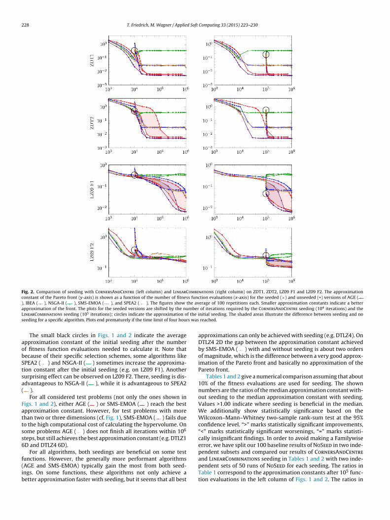
Fig. 2. Comparison of seeding with CornersAndCentre (left column) and LinearCombinations (right column) on ZDT1, ZDT2, LZ09 F1 and LZ09 F2. The approximationconstant of the Pareto front (y-axis) is shown as a function of the number of fitness function evaluations (x-axis) for the seeded (×) and unseeded (+) versions of AGE (), IBEA ( ), NSGA-II ( ), SMS-EMOA ( ), and SPEA2 ( ). The figures show the average of 100 repetitions each. Smaller approximation constants indicate a bettera mberL f the is s was
aobStsa(
Fattss6
f(ib
pproximation of the front. The plots for the seeded versions are shifted by the nuinearCombinations seeding (105 iterations); circles indicate the approximation oeeding for a specific algorithm. Plots end prematurely if the time limit of four hour
The small black circles in Figs. 1 and 2 indicate the averagepproximation constant of the initial seeding after the numberf fitness function evaluations needed to calculate it. Note thatecause of their specific selection schemes, some algorithms likePEA2 ( ) and NSGA-II ( ) sometimes increase the approxima-ion constant after the initial seeding (e.g. on LZ09 F1). Anotherurprising effect can be observed on LZ09 F2. There, seeding is dis-dvantageous to NSGA-II ( ), while it is advantageous to SPEA2
).For all considered test problems (not only the ones shown in
igs. 1 and 2), either AGE ( ) or SMS-EMOA ( ) reach the bestpproximation constant. However, for test problems with morehan two or three dimensions (cf. Fig. 1), SMS-EMOA ( ) fails dueo the high computational cost of calculating the hypervolume. Onome problems AGE ( ) does not finish all iterations within 106
teps, but still achieves the best approximation constant (e.g. DTLZ1D and DTLZ4 6D).
For all algorithms, both seedings are beneficial on some test
unctions. However, the generally more performant algorithmsAGE and SMS-EMOA) typically gain the most from both seed-ngs. On some functions, these algorithms not only achieve aetter approximation faster with seeding, but it seems that all best
of iterations required by the CornersAndCentre seeding (104 iterations) and thenitial seeding. The shaded areas illustrate the difference between seeding and no
reached.
approximations can only be achieved with seeding (e.g. DTLZ4). OnDTLZ4 2D the gap between the approximation constant achievedby SMS-EMOA ( ) with and without seeding is about two ordersof magnitude, which is the difference between a very good approx-imation of the Pareto front and basically no approximation of thePareto front.
Tables 1 and 2 give a numerical comparison assuming that about10% of the fitness evaluations are used for seeding. The shownnumbers are the ratios of the median approximation constant with-out seeding to the median approximation constant with seeding.Values >1.00 indicate where seeding is beneficial in the median.We additionally show statistically significance based on theWilcoxon–Mann–Whitney two-sample rank-sum test at the 95%confidence level. “>” marks statistically significant improvements,“<” marks statistically significant worsenings, “=” marks statisti-cally insignificant findings. In order to avoid making a Familywiseerror, we have split our 100 baseline results of NoSeed in two inde-pendent subsets and compared our results of CornersAndCentre
and LinearCombinations seeding in Tables 1 and 2 with two inde-pendent sets of 50 runs of NoSeed for each seeding. The ratios inTable 1 correspond to the approximation constants after 105 func-tion evaluations in the left column of Figs. 1 and 2. The ratios in
d Soft
Tt
tt)affatiCaa
ttwywrtatd
5
tWvrMq
tehtrihcnusb
A
tDP(
R
[
[
[
[
[
[
[
[
[
[
[
[
[
[
[
[
[
[
[
[
[
T. Friedrich, M. Wagner / Applie
able 2 correspond to the approximation constants after 106 func-ion evaluations in the right column of Figs. 1 and 2.
Counting only the statistically significant results over all func-ions and seedings, the tables show that the majority profits fromhe seeding. The algorithms which benefit the most are SPEA2 (
with 20ד>” and 12ד<”, AGE ( ) with 26ד>” and 20ד<”,nd IBEA ( ) with 24ד>” and 16ד<”. There are significant dif-erences depending on the test function. The LZ09 benchmarkamily profits the most: Summing up the significant results forll algorithms, there are 55ד>” and 15ד<”. Also for DTLZ4here are 21ד>” and 5ד<”. The worst performance of the seed-ng is achieved on the rather difficult WFG functions: While theornersAndCentre seeding achieves over all algorithms 10ד>”nd 6ד<’, the LinearCombinations seeding only achieves 9ד>”nd 29ד<”.
We can do a similar analysis to assess the benefits of the inves-igated seeding approaches. We observe that over all algorithmshe CornersAndCentre seeding yields in total 52ד>” and 27ד<’,hich is a bit better than the LinearCombinations seeding which
ields in total 60ד>” and 46ד<”. In order to answer the questionhether this is statistically significant, we calculate the average
ank of all runs with and without seeding, for each of the 48 func-ions, and each of the 5 algorithms. With this combined data fromll runs, functions and algorithms, the Wilcoxon–Mann–Whitneywo-sample rank-sum test shows significance at the 95% confi-ence level that both seedings improve upon no seeding.
. Conclusions
Seeding can result in a significant reduction of the computa-ional cost and the number of fitness function evaluations needed.
e observe that there is an advantage on many common real-alued fitness functions even if computing an initial seedingeduces the number of fitness function evaluations available for theOEA. For some functions we observe a dramatic improvement in
uality and needed runtime (e.g., DTLZ4 and the LZ09 family).For practitioners, our results show that it can be worthwhile
o apply some form of seeding (especially when evaluations arexpensive), but also to investigate different MOEAs as well, as theyave proven to benefit differently from seeding. While we observedhat seeding can be very beneficial, our experiments could noteveal why this is the case for a particular combination of seed-ng, algorithm, and function landscape. To answer this, many partsave to be studied: the mappings that the benchmark functionsreate from the search spaces into the objective spaces, the con-ectedness between different local Pareto fronts, the adequacy ofsing CMA-ES in the seeding procedure, and much more. As a nexttep towards this goal, we propose to investigate seeding for com-inatorial optimization problems.
cknowledgements
The research leading to these results has received funding fromhe Australian Research Council (ARC) under grant agreementP140103400 and from the European Union Seventh Frameworkrogramme (FP7/2007-2013) under grant agreement no 618091SAGE).
eferences
[1] R.B. Agrawal, K. Deb, Simulated Binary Crossover for Continuous Search Space.
Technical report, 1994.
[2] J. Bader, K. Deb, E. Zitzler, Faster hypervolume-based search using Monte Carlosampling, in: Multiple Criteria Decision Making for Sustainable Energy andTransportation Systems (MCDM ′10), Vol. 636 of Lecture Notes in Economicsand Mathematical Systems, Springer, 2010, pp. 313–326.
[
[
Computing 33 (2015) 223–230 229
[3] K. Bringmann, T. Friedrich, Parameterized average-case complexity of thehypervolume indicator, in: 15th Annual Conference on Genetic and Evolution-ary Computation Conference (GECCO ′13, ACM Press, 2013, pp. 575–582.
[4] K. Bringmann, T. Friedrich, Approximating the volume of unions and intersec-tions of high-dimensional geometric objects, Comput. Geom.: Theory Appl. 43(2010) 601–610.
[5] K. Bringmann, T. Friedrich, Approximating the least hypervolume contribu-tor: NP-hard in general, but fast in practice, Theor. Comput. Sci. 425 (2012)104–116.
[6] K. Bringmann, T. Friedrich, Approximation quality of the hypervolume indica-tor, Artif. Intell. 195 (2013) 265–290.
[7] K. Bringmann, T. Friedrich, F. Neumann, M. Wagner, Approximation-guidedevolutionary multi-objective optimization, in: Proc. 22nd International JointConference on Artificial Intelligence (IJCAI ′11), Barcelona, Spain, 2011, pp.1198–1203, IJCAI/AAAI.
[8] T.C.E. Cheng, A. Janiak, M.Y. Kovalyov, Bicriterion single machine sched-uling with resource dependent processing times, SIAM J. Optim. 8 (1998)617–630.
[9] C. Daskalakis, I. Diakonikolas, M. Yannakakis, How good is the Chord algorithm?in: 21st Annual ACM-SIAM Symposium on Discrete Algorithms (SODA ′10),2010, pp. 978–991.
10] K. Deb, A. Pratap, S. Agrawal, T. Meyarivan, A fast and elitist multiob-jective genetic algorithm: NSGA-II IEEE Trans. Evolut. Comput. 6 (2002)182–197.
11] K. Deb, L. Thiele, M. Laumanns, E. Zitzler, Scalable test problems for evolution-ary multiobjective optimization, in: Evolutionary Multiobjective Optimization,Advanced Information and Knowledge Processing, 2005, pp. 105–145.
12] I. Diakonikolas, M. Yannakakis, Small approximate Pareto sets for biob-jective shortest paths and other problems, SIAM J. Comput. 39 (2009)1340–1371.
13] J.J. Durillo, A.J. Nebro, E. Alba, The jMetal framework for multi-objectiveoptimization: design and architecture, in: IEEE Congress on Evolutionary Com-putation (CEC ′10), 2010, pp. 4138–4325.
14] M.T.M. Emmerich, N. Beume, B. Naujoks, An EMO algorithm using the hyper-volume measure as selection criterion, in: 3rd International Conference onEvolutionary Multi-Criterion Optimization (EMO ′05), Springer, 2005, pp.62–76.
15] Y.G. Evtushenko, M. Potapov, Methods of numerical solution of multicriterionproblem, in: Soviet mathematics – doklady, Vol. 34, 1987, pp. 420–423.
16] M. Gong, L. Jiao, H. Du, L. Bo, Multiobjective immune algorithm with nondom-inated neighbor-based selection, Evolut. Comput. 16 (2008) 225–255.
17] J.J. Grefenstette, Incorporating problem specific knowledge into genetic algo-rithms, Genet. Algorithms Simul. Annealing 4 (1987) 42–60.
18] N. Hansen, The CMA evolution strategy: a comparing review, in: Towards a NewEvolutionary Computation. Advances in Estimation of Distribution Algorithms,Springer, 2006, pp. 75–102.
19] P. Hansen, Bicriterion path problems, in: Multiple Criteria Decision Making:Theory and Applications, Vol. 177 of Lecture Notes in Economics and Mathe-matical Systems, 1980, pp. 109–127.
21] I. Hatzakis, D. Wallace, Dynamic multi-objective optimization with evolution-ary algorithms: a forward-looking approach, in: Proc. 8th Annual Conferenceon Genetic and Evolutionary Computation Conference (GECCO ′06), ACM Press,2006, pp. 1201–1208.
22] A. Hernandez-Diaz, C.A. Coello Coello, F. Perez, R. Caballero, J. Molina, L.Santana-Quintero, Seeding the initial population of a multi-objective evolu-tionary algorithm using gradient-based information, in: Proc. Congress onEvolutionary Computation (CEC ′08), IEEE Press, 2008, pp. 1617–1624.
23] E. Hopper, B. Turton, An empirical investigation of meta-heuristic and heuris-tic algorithms for a 2D packing problem, Eur. J. Oper. Res. 128 (2001)34–57.
24] S. Huband, L. Barone, R.L. While, P. Hingston, A scalable multi-objective testproblem toolkit, in: 3rd International Conference on Evolutionary Multi-Criterion Optimization (EMO ‘05), Vol. 3410 of LNCS, Springer, 2005, pp.280–295.
25] H. Ishibuchi, N. Tsukamoto, Y. Sakane, Y. Nojima, Indicator-based evolutionaryalgorithm with hypervolume approximation by achievement scalarizing func-tions, in: 12th Annual Conference on Genetic and Evolutionary ComputationConference (GECCO ′10), ACM Press, 2010, pp. 527–534.
26] B. Kazimipour, X. Li, A. Qin, Effects of population initialization on differen-tial evolution for large scale optimization, in: Proc. Congress on EvolutionaryComputation (CEC ′14), 2014, pp. 2404–2411.
27] B. Kazimipour, X. Li, A. Qin, A review of population initialization techniques forevolutionary algorithms, in: Proc. Congress on Evolutionary Computation (CEC′14), 2014, pp. 2585–2592.
28] E. Keedwell, S.-T. Khu, A hybrid genetic algorithm for the design of water dis-tribution networks, Eng. Appl. Artif. Intell. 18 (2005) 461–472.
29] H. Li, Q. Zhang, Multiobjective optimization problems with complicated paretosets, MOEA/D and NSGA-II, IEEE Trans. Evolut. Comput. 13 (2009) 284–302.
30] C.-F. Liaw, A hybrid genetic algorithm for the open shop scheduling problem,
Eur. J. Oper. Res. 124 (2000) 28–42.
31] P. Loridan, ε-solutions in vector minimization problems, J. Optim. Theory Appl.43 (1984) 265–276, http://dx.doi.org/10.1007/BF00936165
32] S. Oman, P. Cunningham, Using case retrieval to seed genetic algorithms, Int. J.Comput. Intell. Appl. 1 (2001) 71–82.
33] C.H. Papadimitriou, M. Yannakakis, On the approximability of trade-offs andoptimal access of web sources, in: 41st Annual Symposium on Foundations ofComputer Science (FOCS ′00), IEEE Press, 2000, pp. 86–92.
34] C.H. Papadimitriou, M. Yannakakis, Multiobjective query optimization, in: 20thACM Symposium on Principles of Database Systems (PODS ′01), 2001, pp.52–59.
35] H. Reuter, An approximation method for the efficiency set of multiobjectiveprogramming problems, Optimization 21 (1990) 905–911.
36] G. Ruhe, B. Fruhwirth, ε-optimality for bicriteria programs and its applicationto minimum cost flows, Computing 44 (1990) 21–34.
37] S. Vassilvitskii, M. Yannakakis, Efficiently computing succinct trade-off curves,Theor. Comput. Sci. 348 (2005) 334–356.
38] M. Wagner, T. Friedrich, Efficient parent selection for approximation-guided
evolutionary multi-objective optimization, in: Proc. IEEE Congress on Evolu-tionary Computation (CEC ′13), IEEE, 2013, pp. 1846–1853.
39] M. Wagner, F. Neumann, A fast approximation-guided evolutionary multi-objective algorithm, in: Proc. 15th Annual Conference on Genetic andEvolutionary Computation Conference (GECCO ′13), ACM, 2013, pp. 687–694.
[
Computing 33 (2015) 223–230
40] M. Wagner, K. Bringmann, T. Friedrich, F. Neumann, Efficient optimization ofmany objectives by approximation-guided evolution, Eur. J. Oper. Res. 243(2015) 465–479.
41] M. Yang, X. Zhang, X. Li, X. Wu, A hybrid genetic algorithm for the fitting ofmodels to electrochemical impedance data, J. Electroanal. Chem. 519 (2002)1–8.
42] E. Zitzler, S. Künzli, Indicator-based selection in multiobjective search, in: 8thInternational Conference on Parallel Problem Solving from Nature (PPSN VIII),Vol. 3242 of LNCS, Springer, 2004, pp. 832–842.
43] E. Zitzler, L. Thiele, Multiobjective evolutionary algorithms: a comparative casestudy and the strength Pareto approach, IEEE Trans. Evolut. Comput. 3 (1999)257–271.
44] E. Zitzler, K. Deb, L. Thiele, Comparison of multiobjective evolutionary algo-
45] E. Zitzler, M. Laumanns, L. Thiele, SPEA2. Improving the strength Pareto evo-lutionary algorithm for multiobjective optimization, in: Evolutionary Methodsfor Design, Optimisation and Control with Application to Industrial Problems(EUROGEN 2001), 2002, pp. 95–100.