72
Applied Statistics and Machine Learning Logistic Regression, and Generalized Linear models Model Selection, Lasso, and Structured Sparsity Bin Yu, IMA, June 19, 2013 6/20/13

Applied Statistics and Machine Learning
Logistic Regression, and Generalized Linear models Model Selection, Lasso, and Structured Sparsity Bin Yu, IMA, June 19, 2013
6/20/13

6/20/13 2
Y’s are 0’s and 1’s: challenger data, MISR data Task: relate predictors x’s with Y (1) prediction (IT sector, banking, etc) (2) interpretation: what are the important predictors and they are suggestive for interventions for causal inference later.
Classification is supervised learning

6/20/13 3
These data are from Table 1 of the article "Risk Analysis of the Space Shuttle: Pre-Challenger Predication of Failure" by Dalal, Fowlkes and Hoadley, Journal of the American Statistical Association, Vol. 84, No. 408 (Dec. 1989), pp. 945-957.
I got them from Professor Stacey Shancock at Clark Univ.’s website http://www.math.clarku.edu/~shancock/m110/Challenger_Data.html She has this Tukey quote at her site: "Far better an approximate answer to the right question, than the
exact answer to the wrong question, which can always be made precise." - John Tukey
Challenger data

6/20/13 4
Temp – temperature at launch Failure – number of O-rings that failed Failure1 – indicator of O-ring failure or not
Challenger data

6/20/13 5
Challenger data (jittered)

6/20/13 6
What would you do? A method to fit the data to come up with a prediction rule for the next launch at temp* Postulate a statistical model (e.g. normal reg model) for uncertainty statement
Suppose you are the first person who ever thought about classification problem

6/20/13 7
Fitting methods: nearest neighbor (NN), LS, logistic regression How to fit? what is the criterion to fit? MAXIMUM LIKELILHOOD In the derivations to come, we use notations and some
materials from Dobson (2001).
Suppose you are the first person who ever thought about classification problem

6/20/13 8
Logistic regression model
What does this model mean for the Challenger data? What assumptions might be violated? Which are reasonable?

6/20/13 9
Logistic regression model

6/20/13 10
Logistic regression model

6/20/13 11
Logistic regression model
Note that a linear approximation to U is equivalent to a quadratic approximation to −�(β)

6/20/13 12
Logistic regression model

6/20/13 13
Logistic regression model

6/20/13 14
Logistic regression model vs LS for Challenger data

6/20/13 15
Logistic regression vs LS for Challenger data

6/20/13 16
Generalized Linear Models (GLMs)
GLMs is a statistical framework that unifies normal regression models (for continuous data), logistic (profit) regression models (for binary data), and log linear models (for count data). Logistic (probit) regression models can be also used for multi-class classification. • Original paper on GLMs: Nelder & Wedderburn (1972) GLMs, Journal of Royal Statistical Society- Series A (JRSS-A). Books: • A. J. Dobson (2001): An introduction to GLMs (2nd ed) • P. McCullagh & J. A. Nelder (1999) Generalized linear models (2nd ed) 1

6/20/13 17
Exponential families:

6/20/13 18
A sketch of proof:
HW: derive the formula for V(a(Y)).

6/20/13 19
GLMs: link function is the key to relate response variable to beta in a linear way

6/20/13 20
Likelihood function of a GML

6/20/13 21
Maximum Likelihood Estimation (MLE)

6/20/13 22
Fit a GLM with MLE and then take n samples from the fitted distribution.
Note that this is not the same as the “parametric bootstrap”
described for regression model where we sample from the residuals, not from the fitted normal distribution to the residuals.
Parametric bootstrap works for “nice” parametric families, typically when asymptotic normality holds. For example, bootstrap does not work for Unif(0, a) with a as the parameter.
Non-parametric bootstrap sample directly from observed data.
Parametric bootstrap for GLMs

6/20/13 23
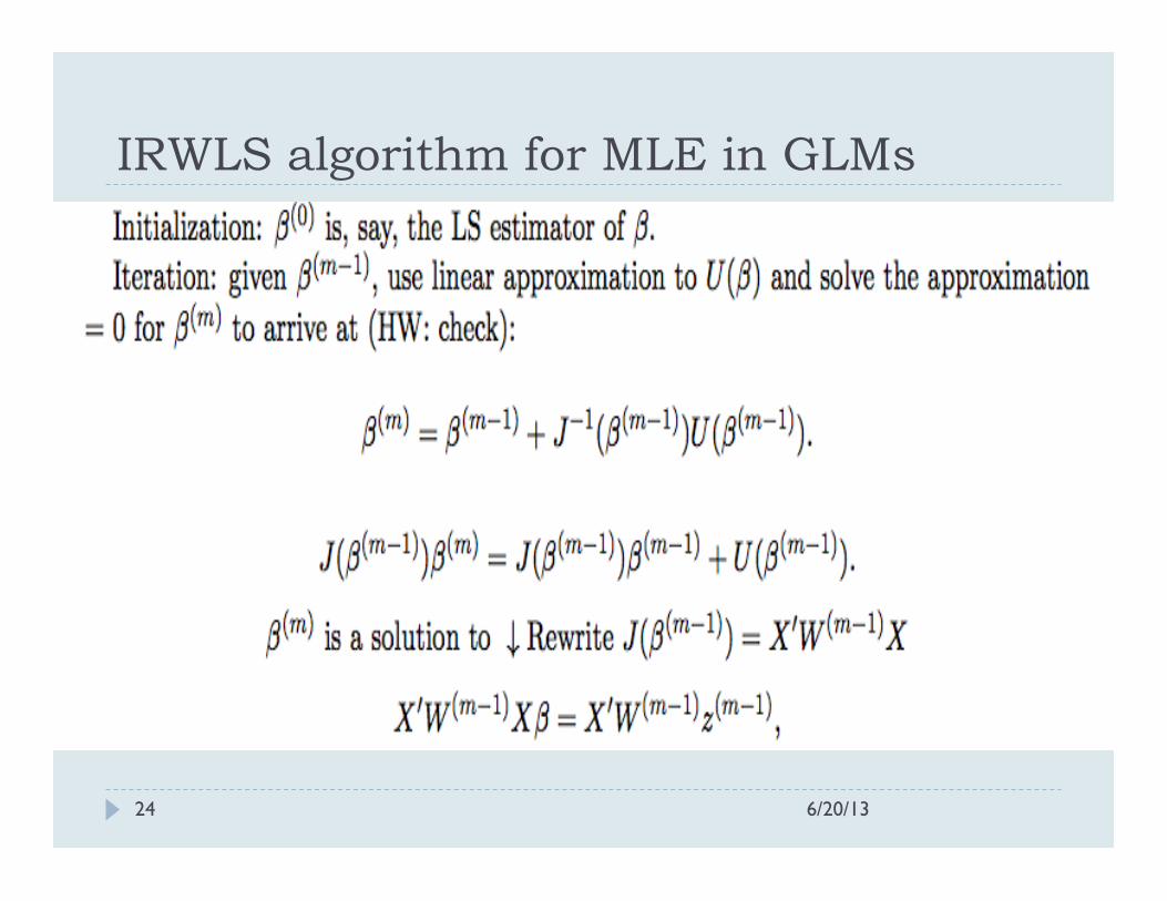
How to compute MLE in GLMs: IRWLS
6/20/13 24
IRWLS algorithm for MLE in GLMs

6/20/13 25
Statistical interpretation of the IRWLS algorithm
Is the solution to a weighted LS problem with weight vector

6/20/13 26
Statistical interpretation of IRWLS

6/20/13 27
IRWLS is an iterative algorithm. At each iteration, IRWLS solves a WLS problem that is the log-
likelihood function of a heteroscedastic linear regression model in the g-domain (where g(mu_i) is approximately linear in \beta),
for which the variances of g(Y_i) are known from the previous iteration.
IRWLS in words

Back to Movie-fMRI Data (Nishimoto et al, 11)
6/20/13 28
7200s training (1 replicate) and 5400s test (10 replicates).

How Stimuli Evoke Brain Signals? } Quantitative models - both stimulus and response high-dimensional
6/20/13 29
Encoding model
Decoding model
Natural Input (Image or video/movie) fMRI of Brain
Dayan and Abbott (2005)

page 30 June 20, 2013 page 30 20 June 2013
Movie reconstruction results for 3 subjects

“Mind-Reading Computers” in Media
6/20/13 31
one of the 50 best inventions of 2011 by Time Magazine Others: Economist, NPR, …

6/20/13 32
What model is behind the movie reconstruction algorithm? Is the model “interpretable” and “reliable”?

Domain knowledge: key for big data discovery
http://cogsci.bme.hu/~ikovacs/ 33
Hubel and Wiesel (1959) discovered, in neuron cells of the primary cortex area V1,
orientation and location selectivity, and
excitatory and inhibitory regions .

Modern Description of Hubel-Wiesel work: Early Visual Area V1
6/20/13 34
} Preprocessing an image:
} Gabor filters corresponding to particular spatial frequencies, locations, orientations (Hubel and
Wiesel, 1959,…)
Sparse representation after Gabor Filters, static or dynamic

page 35 June 20, 2013
2D Gabor Features
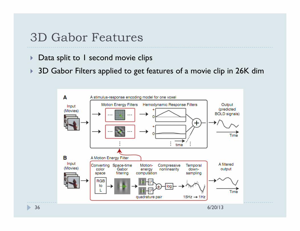
3D Gabor Features
6/20/13 36
} Data split to 1 second movie clips
} 3D Gabor Filters applied to get features of a movie clip in 26K dim

page 37 June 20, 2013
Regularization: key for big data discovery
Two regularization methods are behind the movie reconstruction algorithm, after tons of work for feature construction based on domain knowledge by humans:
} Encoding through L1-penalized Least Squares (LS) or Lasso: Separate sparse linear model fitted to features for each voxel via Lasso (Chen and Dohono, 94; Tibshirani, 96) (cf. e-L2Boosting) } Decoding through L2- or Tikhonov regularization of sample cov.
matrix of residuals across voxels. (cf. Kernel Machines)

page 38 June 20, 2013
Given a voxel, n=7K, p = 26K image 3D wavelet features (each of which has a location)
For each frame, response is the fMRI signal at the voxel. An underdetermined problem since p is much larger than n.

page 39 June 20, 2013
Movie-fMRI: linear encoding model for a voxel
For each voxel and the ith movie clip, we postulate a linear encoding (regression) model: where is the feature vector of movie clip weight vector that combines feature strengths into mean fMRI response is the disturbance or noise term is the fMRI response
Xi = (xi1, xi2, ..., xip)T
Yi = β1xi1 + β2xi2 + ...+ βpxip + �i = XTi β + �i
�iYi
β = (β1,β2, ...,βp)T

page 40 June 20, 2013
Movie-fMRI: finding the weight vector Least Squares: find to minimize Since p = 26,000 >> n=7,200, this LS problem has many solutions.
β1,β2, ...,βp
n�
i=1
(Yi − β1xi1 − β2xi2 − ...− βpxip)2 := ||Y −Xβ||2

Why doesn’t LS work when p>>n?
6/20/13 41
Reason: colinearity of the columns of X -- it also happens in low-dim
Least Squares Function Surfaces as a function of (β1,β2)
How to fix this problem?
6/20/13 42
In general, impossible.
However, in our case, for each voxel, Hubel and Wiesel’s work suggests that only a small number of the predictors among the 26,000 of them be active – sparsity!
This prior information motivates a sparsity-enforced revision to LS:
Lasso = Least Absolute Selection and Shrinkage Operator

page 43 June 20, 2013
Modeling “history” at Gallant Lab
} Prediction on validation set is the benchmark
} Methods tried: neural nets, SVMs, Lasso, …
} Among models with similar predictions, simpler (sparser) models by Lasso are preferred for interpretation This practice reflects a general trend in statistical machine learning -- moving from prediction to simpler/sparser models for interpretation, faster computation or data transmission.

page 44 June 20, 2013
Occam’s Razor 14th-century English logician and Franciscan friar, William of Ockham"
Principle of Parsimony:
Entities must not be multiplied beyond necessity.
Wikipedia

page 45 June 20, 2013
Occam’s Razor via Model Selection in Linear Regression
• Maximum likelihood (ML) is LS with Gaussian assumption
• There are submodels
• ML goes for the largest submodel with all predictors
• Largest model often gives bad prediction for p large

page 46 June 20, 2013
Model Selection Criteria Akaike (73,74) and Mallows (1973) Cp used estimated prediction errors to choose a model (assuming is known):
Schwartz (1980) used asymptotic approximations to negative log posterior probabilities to choose a model (assuming is known)
Both are penalized LS by .
Rissanen’s Minimum Description Length (MDL) principle gives rise to many different different criteria. The two-part code leads to BIC.
(see e.g. Rissanen (1978) and review article by Hansen and Yu (2000))
σ2
σ2

page 47 June 20, 2013
More details on AIC

page 48 June 20, 2013
More details on AIC

page 49 June 20, 2013
More details on AIC
PE = expected Prediction Error

page 50 June 20, 2013
More details on AIC Assume Then PE Hence when p increases, the prediction error increases because a more complex model is being estimated with an associated larger variance. How to use RSS to estimate PE?

page 51 June 20, 2013
More details on AIC

page 52 June 20, 2013
More details on BIC
page 53 June 20, 2013
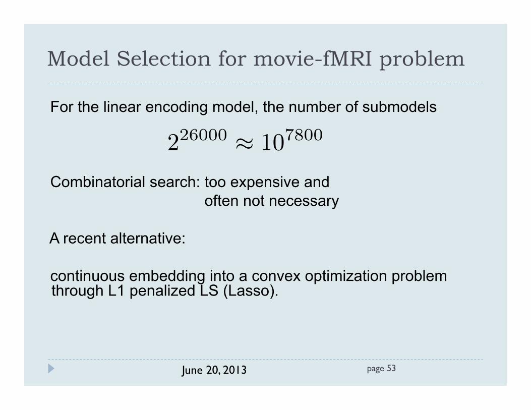
Model Selection for movie-fMRI problem For the linear encoding model, the number of submodels Combinatorial search: too expensive and often not necessary A recent alternative: continuous embedding into a convex optimization problem
through L1 penalized LS (Lasso).
226000 ≈ 107800
page 54 June 20, 2013
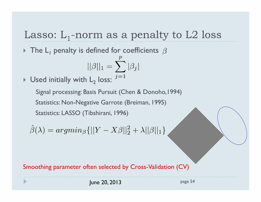
} The L1 penalty is defined for coefficients
} Used initially with L2 loss:
Signal processing: Basis Pursuit (Chen & Donoho,1994)
Statistics: Non-Negative Garrote (Breiman, 1995)
Statistics: LASSO (Tibshirani, 1996)
Smoothing parameter often selected by Cross-Validation (CV)
Lasso: L1-norm as a penalty to L2 loss
β̂(λ) = argminβ{||Y −Xβ||22 + λ||β||1}

Lasso eases the instability problem of LS
6/20/13 55
Lasso Function Surfaces as a function of (β1,β2)

Recall: why doesn’t LS work when p>>n?
6/20/13 56
Reason: colinearity of the columns of X -- it also happens in low-dim
Least Squares Function Surfaces as a function of (β1,β2)

page 57 June 20, 2013
Initially: quadratic program (QP) for each a grid on λ. QP is called for each λ. Later: path following algorithms such as homotopy by Osborne et al (2000) LARS by Efron et al (2004) Current: first-order or gradient-based algorithms for large p (see Mairal’s lecture)
Lasso: computation

page 58 June 20, 2013
Recent theory on Lasso (more in my last lecture)
Under sparse high-dim linear regression model and appropriate conditions:
Lasso is model selection consistent (Irrepresentable condition)
Lasso has optimal L2 estimation rate (restricted eigen value condition)
Selective references: Freund and Schapire (1996), Chen and Donoho (1994), Tibshirani (1996),
Friedman (2001), Efron et al (2004), Zhao and Yu (2006), Meinshausen and Buhlmann (2006),
Wainwright (2009), Candes and Tao (2005), Meinshausen and Yu (2009), Huang and Zhang (2009),
Bickel, Ritove and Tsybakov (2011), Raskutii, Wainwright, and Yu (2010), Neghaban et al (2012)…

Encoding: energy-motion model necessary
59

Encoding: sparsity necessary
60
Sparse regression improves prediction over OLS
(Full-brain data)
0.5 1.0 Prediction accuracy (Full-brain data)
Linear Regression
Sparse Regression

page 61 June 20, 2013
Knowledge discovery: interpreting encoding models
Voxel A Voxel B Voxel C
Lasso+CV CV=Cross- Validation
Prediction scores on Voxels A-C are 0.72 (CV)
Spatial locations of selected features are suggestive of driving factors for brain activities at a voxel.

ES-CV: Statistical Stability (ES) (Lim & Yu, 2013)
6/20/13 62
Given a smoothing parameter , divide the data units into M blocks.
Get Lasso estimate for data with m-th block deleted, and
form an estimate for the mean regression function.
Define the estimation stability (ES) measure as
which is the reciprocal of a test statistic for testing
λ
β̂m(λ)
¯̂β(λ) =1
M
�
m
β̂m(λ)
Xβ̂m(λ)
ES(λ) =1M
�m ||Xβ̂m(λ)−X ¯̂β(λ)||2
||X ¯̂β(λ)||2
H0 : Xβ = 0

ES-CV (or SSCV): Estimation Stability (ES)+CV (continued)
6/20/13 63
ES-CV selection criterion for smoothing parameter : Choose the that minimizes and is not smaller that the CV selection.
Related works: Shao (95), Breiman (96), …
Bach (08), Meinshausen and Buhlmann (2008), …
λ
λ
ES(λ)

page 64 June 20, 2013
Back to fMRI prblem: Spatial Locations of Selected Features
Voxel A Voxel B Voxel C
CV
ES-CV
Prediction on Voxels A-C: CV 0.72, ES-CV 0.7

page 65 June 20, 2013
ESCV: Sparsity Gain (60%) with No Prediction Loss (-1.3%)
Prediction (correlation)
Model size
CV
SSC
V
SSC
V
CV % Change
% Change
Based on validation data for 2088 voxels

ES-CV: Desirable Properties
6/20/13 66
CV (cross-validation) is widely used in practice.
ES-CV is an effective improvement over CV on stability and hence interpretability and reliability of results. § Computational cost similar to CV § Easily parallelizable as CV § Empirically sensible or nonparametric Other forms of perturbation include: sub-sampling, bootstrap, variable permutation, ...

page 67 June 20, 2013
Structured sparsity: Composite Absolute Penalties (CAP) (Zhao, Rocha and Yu, 09)
Motivations: } side information available on predictors and/or } sparsity at group level } extra regularization need (p>>n) than what Lasso provides
} Examples of groups: } Genes belonging to the same pathway; } Categorical variables represented by “dummies”; } Noisy measurements of the same variable.
} Examples of hierarchy:
} Multi-resolution/wavelet models; } Interactions terms in factorial analysis (ANOVA); } Order selection in Markov Chain models. Existing works can be seen as special cases of CAP: Elastic Net (Zou & Hastie, 05), GLASSO (Yuan & Lin, 06), Blockwise Sparse Regression (Kim, Kim & Kim, 2006)

page 68 June 20, 2013
Norm Lγ
Bridge Parameter γ ¸ 1

page 69 June 20, 2013
} The CAP parameter estimate is given by:
} Gk's, k=1,…,K - indices of k-th pre-defined group
} βGk – corresponding vector of coefficients.
} || . ||γk – group Lγ
k norm: Nk = ||βγ
k||γ
k;
} || . ||γ0 – overall norm: T(β) =||N||γ
0
} groups may overlap (hierarchical selection)
Composite Absolute Penalties (CAP)

page 70 June 20, 2013
CAP Group selection
} Tailoring T(β) for group selection: } Define non-overlapping groups } Set γk>1
} Group norm γk tunes similarity within its group } γk>1 encourages all variables in group i to be included/
excluded together } Set γ0=1:
} This yields grouped sparsity } γi=2 has been studied by Yuan and Lin (Grouped Lasso, 2005).

page 71 June 20, 2013
} Tailoring T(β) for Hierarchical Structure:
} Set γ0=1
} Set γi>1, ∀i
} Groups overlap:
} If β2 appears in all groups where β1 is included
Then X2 is encouraged to enter the model after X1
} As an example:
CAP Hierarchical Structures

page 72 June 20, 2013
CAP: a Bayesian interpretation
} For non-overlapping groups:
} Prior on group norms:
} Prior on individual coefficients:


