Applied Survey Data Analysis

Module 2: Variance Estimation

March 30, 2013

Applied Statistics Lab

Approaches to Complex Sample

Variance Estimation

• In simple random samples many estimators are linear estimators where the sample size n is fixed. A linear estimator is a linear function of the sample observations.

• When survey data are collected using a complex design with unequal size of clusters or when weights are used in estimation, most statistics of interest will not be simple linear function of the observed data.

Where:

𝑦ℎ∝𝑖 =Measurement on unit 𝑖 in cluster α in stratum ℎ

𝑤ℎ∝𝑖 =Corresponding weight

Two approaches

• Replication or Resampling Methods technique:

-Jackknife Repeated Replication

-Balanced Repeated Replication

• Taylor Series approximation or linearization technique:

-Approximate nonlinear statistics as a linear function of sample totals

-Specific form of the variance estimator for each statistic

Replication Methods

• Replication methods use information on variability between

estimates drawn from different subsamples of an overall sample to

make inferences about variance in the population

• Steps in Replicated Methods:

1. A defined number (K) of subsets (replicate samples) of the full

sample are selected.

2. Create revised weight for replicate sample.

3. Compute weighted estimates of population statistic of interest

for each replicate using replicate weight.

4. The variability between these subsample replicate statistics are

used to estimate the variance of the full sample statistic.

Jackknife Repeated Replication (JRR)

• The Jackknife Repeated Replication (JRR) is applicable

to a wide range of complex sample designs including

designs in which two or more PSUs are selected from

each of h=1,…,H primary stage strata.

• Using Jackknife for unstratified surveys, one PSU at a

time is omitted from the sample and the others

reweighted to keep the same total weight (known as the

JK1 Jackknife).

• For stratified designs, Jackknife removes one PSU at a

time, but reweights only the other PSUs in the same

stratum.

JRR: Constructing Replicates, Replicate

Weights

• Suppose there are H strata with ah clusters.

• Each replicate is constructed by deleting one or more

PSUS from a single stratum

• Replicate weight values for cases in the deleted PSUs

are assigned a value of “0” or “ missing”

• The replicate weight for each replicate multiplies the

weights for remaining cases in the deleted stratum by a

factor of ah /[ah -1].

• Replicate 1 weight values remain unchanged for cases in

all other strata.

JRR: Constructing Replicates, Replicate

Weights (2)

• Each Stratum will contribute ah-1 unique JRR replicates,

yielding a total of

𝑅 = 𝑎ℎ − 1

𝐻

ℎ=1

= 𝑎 − 𝐻 = #𝑐𝑙𝑢𝑠𝑡𝑒𝑟𝑠 − #𝑠𝑡𝑟𝑎𝑡𝑎

JRR: Constructing Estimates

• The weighted estimate for each of r=1,…R replicates:

• The full sample estimate of the mean is:

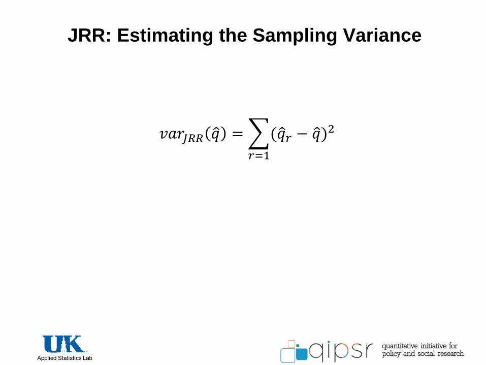
JRR: Estimating the Sampling Variance

𝑣𝑎𝑟𝐽𝑅𝑅 𝑞 = (𝑞 𝑟 − 𝑞 )2

𝑟=1

Balanced Repeated Replication(BRR)

• Balanced Repeated Replication (BRR) is a half-sample method

that was developed specifically for estimating sampling variances

under two PSU- per-stratum sample designs.

• A half sample is defined by choosing one PSU from each stratum.

• A complement of a half sample is made up of all those PSUs not in

the half sample. A complement is also a half sample.

• There are 2H possible half samples and their complements. We only

need H half samples for variance estimation.

Hadamard Matrix for a H=4 strata design

BRR

Replicate

Stratum

1 2 3 4

1 + + + -

2 + - - -

3 - - + -

4 - + - -

BRR: Constructing Replicates and Replicate

Weights

• H replicates are created based on the deletion pattern ( + and -) in

the Hadamard matrix

• Replicate weight is then created for each of the h=1,…, H BRR

sample replicates.

• Replicate weight values for cases in the complement half-sample

PSUs are assigned a value of “0” or “ missing”

• Replicate weight values for the cases in the PSUs retained in the

half-sample are formed by multiplying the full sample analysis

weights by a factor of 2.

BRR: Constructing Estimates

• The weighted estimate for each of r=1,…R replicates:

• The full sample estimate is:

BRR: Estimating the Sampling Variance

𝑣𝑎𝑟𝐵𝑅𝑅 𝑦 𝑤 = 𝑣𝑎𝑟𝐵𝑅𝑅 𝑞 =1

𝑅 (𝑞 𝑟 − 𝑞 )2

𝑅

𝑟=1

Balanced Repeated Replication

• Pro

– Relatively few computations

– Asymptotically equivalent to linearization

methods for smooth functions of population

totals and quantiles

• Con

– 2 psu per stratum

Linearization (Taylor Series Method)

• Linearization techniques make mathematical

adjustments so that standard ‘linear estimators’

can be applied to data.

• Linearization is a widely used technique for

estimating variance of any functions of the

weighted totals. These include ratios, subgroup

differences in the ratios, regression coefficients

and correlation coefficients.

Taylor Series Linearization

, ,

2 2

( , ) ( , ) ( ) ( )

var( ( , )) var( ) var( ) 2 cov( , )

o o o o

o o o o

x x z z x x z z

f ff x z f x z x x z z

x z

f x z A x B z AB x z

A B

2

2

2

( , )

1

( ) ( ) 2 ( , )

o

o

o

o

o

o

xf x z

z

fA

x z

xfB

z z

x Var x R Var z R Cov x zVar

z z

xR

z

The estimates under TSL

• Consider the weighted estimates of the population mean of variable y

• Rewriting it as a linear combination of weighted sample totals using TSL

𝑦 𝑤,𝑇𝑆𝐿 =𝑢0

𝑣0+ 𝑢 − 𝑢0

𝜕𝑦 𝑤,𝑇𝑆𝐿

𝜕𝑢 𝑢=𝑢0,𝑣=𝑣0

+ 𝑣 − 𝑣0𝜕𝑦 𝑤,𝑇𝑆𝐿

𝜕𝑣 𝑣=𝑣0,𝑢=𝑢0

+ 𝑟𝑒𝑚𝑎𝑖𝑛𝑑𝑒𝑟

𝑦 𝑤,𝑇𝑆𝐿 = 𝑢0

𝑣0+ 𝑢 − 𝑢0

𝜕𝑦 𝑤,𝑇𝑆𝐿

𝜕𝑢 𝑢=𝑢0,𝑣=𝑣0

+ 𝑣 − 𝑣0𝜕𝑦 𝑤,𝑇𝑆𝐿

𝜕𝑣 𝑣=𝑣0,𝑢=𝑢0

𝑦 𝑤,𝑇𝑆𝐿 = 𝑐𝑜𝑛𝑠𝑡𝑎𝑛𝑡 + 𝑢 − 𝑢0 ∙ 𝐴 + 𝑣 − 𝑣0 ∙ 𝐵

Where

𝐴 =𝜕𝑦 𝑤,𝑇𝑆𝐿

𝜕𝑢 𝑢=𝑢0,𝑣=𝑣0

=1

𝑣0; 𝐵 =

𝜕𝑦 𝑤,𝑇𝑆𝐿

𝜕𝑣 𝑢=𝑢0,𝑣=𝑣0

= −𝑢0

𝑣02 ;

The Variance under TSL

• The approximate variance of the “ linearized’ form of the estimate

𝑦 𝑤,𝑇𝑆𝐿

Where:

𝐴 =𝜕𝑦 𝑤,𝑇𝑆𝐿

𝜕𝑢 𝑢=𝑢0,𝑣=𝑣0

=1

𝑣0; 𝐵 =

𝜕𝑦 𝑤,𝑇𝑆𝐿

𝜕𝑣 𝑢=𝑢0,𝑣=𝑣0

= −𝑢0

𝑣02 ; 𝑎𝑛𝑑

𝑢0, 𝑣0 𝑎𝑟𝑒 𝑡ℎ𝑒 𝑤𝑒𝑖𝑔ℎ𝑡𝑒𝑑 𝑠𝑎𝑚𝑝𝑙𝑒 𝑡𝑜𝑡𝑎𝑙𝑠 𝑐𝑜𝑚𝑝𝑢𝑡𝑒𝑑 𝑓𝑟𝑜𝑚 𝑡ℎ𝑒 𝑠𝑢𝑟𝑣𝑒𝑦 𝑑𝑎𝑡𝑎.

• Therefore, the sampling variance of the nonlinear estimate 𝑦 𝑤,𝑇𝑆𝐿 is

approximated by a simple algebraic function of quantities that can

be readily computed from the complex sample survey data.

𝑣𝑎𝑟 𝑦 𝑤,𝑇𝑆𝐿 = 𝑣𝑎𝑟 𝑢 + 𝑦 𝑤,𝑇𝑆𝐿

2 ∙ 𝑣𝑎𝑟 𝑣 − 2 ∙ 𝑦 𝑤,𝑇𝑆𝐿 ∙ 𝑐𝑜𝑣(𝑢, 𝑣)

𝑣02

𝑣𝑎𝑟 𝑦 𝑤,𝑇𝑆𝐿 = 𝑣𝑎𝑟 𝑐𝑜𝑛𝑠𝑡𝑎𝑛𝑡 + 𝑢 − 𝑢0 ∙ 𝐴 + 𝑣 − 𝑣0 ∙ 𝐵

= 0 + 𝐴2𝑣𝑎𝑟 𝑢 − 𝑢0 + 𝐵2𝑣𝑎𝑟 𝑣 − 𝑣0 + 2𝐴𝐵𝑐𝑜𝑣(𝑢 − 𝑢0, 𝑣 − 𝑣0) = 𝐴2𝑣𝑎𝑟 𝑢 + 𝐵2𝑣𝑎𝑟 𝑣 + 2𝐴𝐵𝑐𝑜𝑣(𝑢, 𝑣)

Linearization

(Taylor Series Methods)

• Pro:

• Linearization technique is useful if the estimate can be

expressed as a function of sample totals

• Theory is well developed

• The default is most software package for complex samples

• Con:

• Finding partial derivatives may be difficult

• Different method is needed for each statistic

• The function of interest may not be expressed a smooth

function of population totals or means

• Accuracy of the linearization approximation

Applied Statistics Lab