Page 1
APPRAISAL OF CREDIT APPLICANT USING LOGISTIC AND
LINEAR DISCRIMINANT MODELS WITH PRINCIPAL
COMPONENT ANALYSIS
BY
CHRISTOPHER WANYONYI KIVEU
I56/69357/2013
THIS PROJECT IS SUBMITTED IN PARTIAL FULFILMENT OF
THE REQUIREMENT FOR THE AWARD OF THE DEGREE OF
MASTERS IN SOCIAL STATISTICS, SCHOOL OF
MATHEMATICS AT THE UNIVERSITY OF NAIROBI
JUNE 2015
Page 2
ii
DECLARATION
Declaration by the student
This research project is my original work and to the best of my knowledge has not been
presented to any other examination body. No part of this research work should be
produced unless for learning purposes without my consent or that of University of
Nairobi.
Signature……………………….. Date……………………..
Christopher Wanyonyi Kiveu
I56/69357/2013
Declaration by the Supervisors
This research project has been submitted for examination with my approval as the
university Supervisor.
Signature……………………………….. Date………………………….
Prof. Ganesh P. Pokhariyal
Page 3
iii
ACKNOWLEDGEMENTS
I give thanks and all the glory to almighty God for the grace, strength, wisdom, provision
and good health He has given me while doing this project.
Special thanks to Prof. Ganesh P. Pokhariyal, who has been a critical, diligent and
focused reviewer of my work. Thank you for the good guidance and inspiration you
rendered to me. I am motivated by the passion you have for research and academic
excellence. I would also like to thank Dr. Awiti for his keen interest and motivation on
how to go about the analysis. Your support was not in vain.
In addition, I would like to thank dad, Paul K. Buyavo and mum, Peritah Kiveu for the
love, support, care and encouragement. I would not have been what I am today without
you. Thank you for raising me up. To my brothers and sisters, thanks for your
encouragement and motivation. I am blessed being part of you.
To my lovely fiancé Ruth J. Cheruiyot, thank you for being there for me. Your support,
prayers and encouragements were not in vain. Finally, special thanks to my friends and
classmates Zachary Ochieng and Tom Omyonga, your encouragement and team spirit
was superb. Thank you!
Page 4
iv
DEDICATION
I wish to dedicate this project to: -
The love of my life and my best friend, Ruth J. Cheruiyot.
My brothers and sisters.
Dear parents: Paul Buyavo and Peritah Kiveu.
Page 5
v
TABLE OF CONTENTS
DECLARATION ................................................................................................................ ii
ACKNOWLEDGEMENTS ............................................................................................... iii
DEDICATION ................................................................................................................... iv
TABLE OF CONTENTS .....................................................................................................v
LIST OF TABLES ............................................................................................................ vii
LIST OF FIGURES ......................................................................................................... viii
LIST OF ABBREVIATIONS ............................................................................................ ix
ABSTRACT .........................................................................................................................x
CHAPTER ONE: INTRODUCTION ..............................................................................1
1.1 Background ....................................................................................................................1
1.2 Research Problem ..........................................................................................................4
1.3 Objectives of the Study ..................................................................................................4
1.4 Significance of the study ...............................................................................................5
CHAPTER TWO: LITERATURE REVIEW .................................................................7
2.1 Introduction ....................................................................................................................7
2.2 Conclusion ...................................................................................................................14
CHAPTER THREE: METHODOLOGY .....................................................................17
3.0 Introduction ..................................................................................................................17
3.1 Data description ..........................................................................................................18
3.2 Principal Component Analysis (PCA) ........................................................................18
3.2.1 Basic assumptions (PCA) ................................................................................. 20
3.2.2 Summary of PCA approach .............................................................................. 20
3.3 Binary Logistic Regression .........................................................................................21
3.3.1 Basic assumptions of Binary Logistic Regression ........................................... 22
3.4 Linear Discriminant Analysis (LDA) ..........................................................................23
3.4.1 Basic assumptions (LDA) ................................................................................. 25
Page 6
vi
3.4.2 Summary the LDA approach ............................................................................ 26
3.5 Hypothesis testing ........................................................................................................26
3.5.1 KMO and Bartlett’s test .................................................................................... 26
3.5.2 Wilks’ Lambda Test for significance of canonical correlation: ....................... 27
3.5.3 Chi-square Test ................................................................................................. 28
3.5.4 Omnibus Chi-square Test ................................................................................. 28
3.5.5 Box M Test for the Equality of Covariance Matrices ...................................... 29
3.5.6 Wald Test .......................................................................................................... 29
CHAPTER FOUR: DATA ANALYSIS AND RESULTS ............................................31
4.1 Introduction ..................................................................................................................31
4.2 PCA output...................................................................................................................32
4.3 Data Analysis output using Binary Logistic Model .....................................................35
4.4 Data Analysis Output Using Linear Discriminant .......................................................40
CHAPTER FIVE: CONCLUSIONS AND RECOMMEDATIONS ...........................47
5.1 Introduction ..................................................................................................................47
5.2 Predictive Models Comparison ....................................................................................48
5.3 Discussion ....................................................................................................................49
5.4 Recommendations ........................................................................................................50
REFERENCES .................................................................................................................52
Page 7
vii
LIST OF TABLES
Table 3.1: Credit Dataset Description ................................................................................18
Table 4.1: KMO Statistics for Sampling Adequate and Bartlett’s test for Homogeneity ..31
Table 4.2: PCA Total Variance Explained ........................................................................32
Table 4.3: The Coefficient of Principal Component Score of Variables ...........................34
Table 4.4: Classification table step 0 .................................................................................36
Table 4.5: Variables not in the equation step 0 ..................................................................36
Table 4.6: SPSS output: Model Test: .................................................................................37
Table 4.7: Model Summary ...............................................................................................37
Table 4.8: SPSS Output: Logistic Classification Table .....................................................38
Table 4.9: SPSS Output: Important variables in Logistic Regression ...............................38
Table 4.10: SPSS Output: Tests of Equality of Group Means in Discriminant Analysis ..40
Table 4.11: Test Results of Box’s M .................................................................................41
Table 4.12: Eigenvalues .....................................................................................................41
Table 4.13: Wilks' Lambda ................................................................................................42
Table 4.14: Classification Function Coefficients ...............................................................42
Table 4.15: Canonical Discriminant Function Coefficients ..............................................43
Table 4.16: Group centroids table ......................................................................................44
Table 4.17: Prior Probabilities for Groups .........................................................................45
Table 4.18: SPSS Output: Discriminant Analysis Classification Results..........................45
Page 8
viii
LIST OF FIGURES
Figure 4.1: Scree Plot for the Principal components output ..............................................33
Page 9
ix
LIST OF ABBREVIATIONS
PCA Principal Component Analysis
LR Logistic Regression
LDA Linear Discriminant Analysis
PC Principal Components
CS Credit Score
CF Credit Factor
Page 10
x
ABSTRACT
In this project, we examine the criteria for classify credit applicant status using Binary
Logistic Regression and Linear Discriminant models with Principal Components as input
variables for predicting applicant status in terms of Creditworthy or Non- creditworthy.
Information collected for previous credit applicants is used to develop the models for
predicting the new applicant’s creditworthiness. The results obtained showed that the use
of Credit factors obtained from Principal Components as input variables for Linear
Discriminant (LDA) and Logistics Regression (LR) models prediction eliminated
data co-linearity and reduced complexity in dimensionality by grouping variables
together with little loss of information. Based on Eigen values with values above 1, seven
factors were retained. The factors accounted for 76.09 percent of the total variation. One
thousand credit applicants were considered; 715 as creditworthy and 285 as un-
creditworthy. The result obtained from the analysis showed that Logistic Regression gave
classification accuracy 87% slightly better than discriminant analysis 85.60%. However,
discriminant analysis achieved less cost of misclassification 48 than Logistic regression
72 for non-creditworthy applicants classified from the 1000 applicants.
Page 11
1
CHAPTER ONE
INTRODUCTION
1.1 Background
Applicants regularly request for credit facilities from lending institution. A lender
normally makes two types of decisions; whether to grant credit to a new applicant or not
and how to deal with existing applicants; whether to increase their credit limits or not.
The risk to extend the requested credit depends on how well they distinguish the
creditworthiness of the applicants.
Poor evaluation of credit risk can cause huge financial losses to the lenders. Recently,
there has been a sharp increase in non-performing loan by lending institutions despite the
growth in there loan books. This provides a major threat to successful lending despite
advancements in portfolio diversification. Lahsasna et al. (2010) emphasized that credit
risk decisions are key determinants for the success of financial institutions because of
huge losses that result from wrong decisions. Wu et al. (2010) stressed that credit risk
assessment is the basis of credit risk management in commercial banks and provides the
basis for loan decision-making. One widely adopted technique for solving this
classification problem is by using Credit Scoring.
Credit scoring is the set of decision models with underlying techniques that assist lenders
in the granting of consumer credit. These techniques are used in making the decision of
whom to grant credit, how much, how much interest to be charged and what operational
strategies will enhance the profitability of the borrowers to the lenders. Besides, it assists
in assessing the risk in lending. These techniques are a dependable assessment of a
Page 12
2
person’s creditworthiness since they are based on actual data collected. The main
objective here is normally to captures the relationship between the historical information
and future credit performance of the applicants.
It is important that a large sample of previous customers with their application details,
behavioral patterns, and subsequent credit history be available. These samples are used to
identify the connection between the characteristics of the consumers’ e.g. net income,
age, loan amount, number of years in employment with their current employer and how
their subsequent credit history is. Typical application areas in the consumer market
include: credit cards, unsecured personal loans, home mortgages, secured personal loans,
asset finance, and a wide variety of personal and business loan products.
Currently, the uptake of retail credit in financial institutions is extremely high. Besides,
credit is easily accessible to the largest part of the population because of the emerging
trends of internet and mobile banking. As a result, many Financial Institutions are in the
process of setting up credible evaluation systems (credit analysis, credit scoring systems)
in order to facilitate their managers’ decisions to accept or reject applicant’s credit
application quicker and accurately.
In Kenya, the recent increase in non-performing loans has aroused increasing attention on
credit risk prediction and assessment. The decision to grant credit to an applicant has
traditionally been based upon subjective judgments made by human experts, using past
experiences and some guiding principles. The common practice was to consider the
classic credit C’s: character, capacity, capital, collateral and conditions (Abrahams and
Zhang, 2008). This method suffers from high training costs, frequent incorrect decisions,
Page 13
3
inability to handle large volumes in a short period of time and inconsistent decisions
made by different experts for the same application. These shortcomings have led to a rise
in more formal and accurate methods to assess the risk of default.
In this context, automatic determination of credit score and applicant status using models
has become a primary tool for financial evaluation of credit risk, thus reduce possible
loan default risks, and make managerial decisions. This project will focus mainly on
classifying and predicting applicant’s status with the ultimate goal of determining
applicant creditworthiness and discriminate between ‘good’ and ‘bad’ debts, depending
on how likely applicants are to default with their repayments. Compared with the
subjective methods, automatic applicant status models present a number of advantages
i.e. reduction in the cost of the credit evaluation process and the expected risk of being a
bad loan, saving on time, effort, headcount, consistent recommendations based on
objective information and eliminating human biases and prejudices.
Credit applicants’ status models’ summarizes available relevant information about
consumers’ creditworthiness status and reduces the information into a set of binary
categorical outcome that foretell an outcome as either “Credit-worth” or “Un-credit-
worth”. An applicant status is a categorical snapshot of his or her estimated risk profile at
that point in time. The most classical approaches to credit applicant status prediction
employ statistical methods. Namely: discriminant analysis (DA), Logistic Regression
(LR), multivariate adaptive regression splines (MARS), classification and regression tree
(CART). Besides, we have more sophisticated techniques belonging to the area of
computational intelligence (often referred to as data mining or soft computing) such as
neural networks(NNs), support vector machines(SVM), fuzzy systems, rough sets,
Page 14
4
artificial immune systems, and evolutionary algorithms. For the purpose of this project
we will considered two models, namely: Discriminant and Logistic models.
The selection of the independent variables is very essential in the model development
phase because it determines the attributes that decide the value of the credit score. The
values of the independent variables are normally collected from the application
information provided.
1.2 Research Problem
Misclassification of credit applicant has been a major challenge in credit risk
management. Granting credit to applicants who are non-creditworthy can result to huge
financial losses while not granting credit to creditworthy applicants might result to loss of
income. The main challenge remains; how to formulate and select statistical models that
best minimization the bad risk (credit defaulting) and maximize the good risk (good
creditors) for the given datasets. This project focuses on how to develop Logistic and
Discriminant models that will be used to classify and predict credit applicant status.
1.3 Objectives of the Study
The main objective of this study was to develop Logistic and Discriminant models using
Principal components as predictor variables in classifying and predicting credit applicant
status.
Page 15
5
The specific objectives were to:
i. Obtain credit factors that determine the creditworthiness of credit applicants using
PCA.
ii. Develop a binary LR and LDA model for classifying credit applicants as either
creditworthy or non-creditworthy.
iii. Build a LDA and Binary LR model capable of predicting applicant status using
credit factors obtained from PCA as inputs variables.
iv. Compare the classification accuracy of LDA and LR.
1.4 Significance of the study
This study will give insights to lending institutions on prudent credit risk management by
assisting in:-
i. Recommending institutions to charge different interest rates to customers
depending on the credit score instead of basing on the product offered. Customers
with higher credit scores consider charging low interest rates while those with low
credit scores consider charging high interest rates.
ii. Minimization of bad credit risk and maximization good credit risk to the financial
institutions by use of statistical models in estimation and prediction of applicant
status.
iii. Risk selection and assessment to the financial institutions using data driven
models by assessing there classification accuracy.
iv. Elimination of human biasness and prejudice by the financial institutions to
customers’ applications since the status prediction is modeled uniformly.
Page 16
6
v. Automation in the credit systems thus help save on loan processing time, cutting
on costs and Leaning on value-add processes as a result of leveraging on
technology.
The structure of this project is as follows: Chapter 2 discusses the Literature Review.
Chapter 3 describes the methodology, models and definitions of variables. Chapter 4
presents data analysis and results. Finally, Chapter 5 provides the conclusions, discussion
and recommendations.
Page 17
7
CHAPTER TWO
LITERATURE REVIEW
2.1 Introduction
A Good designed model should have higher classification accuracy to classify the new
applicants or existing customers as either good or bad. This is the core purpose of credit
applicants status modelling. Statistical methods like discriminant analysis, factor analysis,
decision tree and logistic regression are the most popular method used for applicant’s
classification.
Discriminant analysis is a parametric statistical technique, developed to discriminate
between two groups. Many researchers have agreed that the discriminant approach is still
one of the most broadly established techniques to classify customers as either good or bad
creditors. This technique has been applied in the credit scoring applications under
different fields and was first proposed by Fisher (1936) as a discrimination and
classification technique. Durand (1941) developed one of the first credit scoring models
using simple parametric statistical model. The appropriateness of LDA for credit scoring
has been in question because of the categorical nature of the credit data and the fact that
the covariance matrices of the good and bad credit classes are not likely to be equal and
credit data not normally distributed. Reichert reports this may not be a critical limitation
(Reichert et al. 1983). However, to overcome this, the categorical variables can be
recorded into binary dummy variables before the analysis. In addition, these assumptions’
should be verified before the use of this model.
Page 18
8
More sophisticated models are being investigated today to overcome some of the
deficiencies of the LDA model. A well-known application in corporate bankruptcy
prediction is one by Altman (1968), who developed the first operational scoring model
based on five financial ratios, taken from eight variables from corporate financial
statements. He produced a Z-Score, which was a linear combination of the financial
ratios. Several authors have expressed pointed criticism of using discriminant analysis in
credit scoring. Eisenbeis (1978) noted a number of the statistical difficulties in applying
discriminant analysis based on his earlier work in 1977. Complications, such as using
linear functions instead of quadratic functions, groups’ definition, prior probabilities
inappropriateness, classification error prediction and others, should be considered when
applying discriminant analysis. Regardless of these problems, discriminant analysis is
still one the most commonly used techniques in credit scoring (Greene, 1998; Abdou et
al. 2009).
Grablowsky (1975) conducted a two-group stepwise discriminant analysis in modeling
risk on consumer credit by using behavioral, financial, and demographic variables. The
data was collected from 200 borrowers through a questionnaire and the loan application
forms of the same 200 borrowers. The analysis started with 36 variables and after a
comprehensive sensitivity analysis, it was found out that 13 variables were adequate to
model the consumer credit risk. Although the data violated the equal variance-covariance
assumptions, the estimated model classified the validation sample 94 per cent correctly.
Page 19
9
Logistic regression is also one of the most widely used statistical techniques in credit
scoring. What distinguishes a logistic regression model from a linear regression model is
that the outcome variable in logistic regression is dichotomous in nature.
Martin (1977) first introduced the logistic regression method to the bank crisis early
warning classification. Martin chose to use data between 1970 and 1976, with 105
bankrupt companies and 2058 non-bankrupt companies in the matching sample, and
analyzed the bankruptcy probability interval distribution, with two types of errors and the
relationship between the split points; he then found that size, capital structure, and
performance were key indexes for the judgment. Martin determined that the accuracy rate
of the overall classification could reach 96.12%. Logistic regression analysis had
significant improvements over discriminant analysis with respect to the problem of
classification. Martin also noted that logistic regression could overcome many of the
issues with discriminant analysis, including but not limited to the assumption of
normality.
Hand & Henley (1997) reviewed available credit scoring techniques including the
available quantitative methods such as logistic regression, mathematical programming,
discriminant analysis, regression, recursive partitioning, expert systems, neural networks,
smoothing nonparametric methods, and time varying models were put in view. They
concluded that there was no best method and remarked that the best method depends
largely on the data structure and its characteristics. They also found out that
characteristics typical to differentiate the good and bad customer are: time at present
address, home status, telephone, applicant’s annual income, credit card, and types of bank
account, age, and country code judgment, types of occupation, purpose of loan, marital
Page 20
10
status, time with bank and time with employers. Parameter estimation for the model is
done using the maximum likelihood method (Freund & William, 1998). On theoretical
grounds, logistic regression is suggested as an appropriate statistical method, given that
the two classes “good” credit and “bad” credit have been described (Hand & Henley,
1997). This model has been expansively been used in credit scoring applications (for
example: Abdou, et al., 2008; Crook et al, 2007; Baesens et al, 2003; Lee & Jung, 2000;
Desai et al, 1996; Lenard et al, 1995).
David West (2000) investigated the credit scoring accuracy of five neural network
models: multilayer perceptron, mixture-of-experts, radial basis function, learning vector
quantization, and fuzzy adaptive resonance. The results obtained were benchmarked
against more traditional methods under consideration for commercial applications
including linear discriminant analysis, logistic regression, k nearest neighbor, kernel
density estimation, and decision trees. West reported Logistic regression as the most
accurate of the traditional methods.
Additionally, West (2000) studied the potential of five neural network architectures in
credit scoring accuracy and benchmarked the results with traditional statistical methods:
linear discriminant analysis and logistic regression, and other non-parametric methods:
decision trees, kernel density estimation, and nearest neighbor. The results obtained
showed that neural networks credit models were able to improve credit scoring accuracy
by 3%.
Lee et al. (2002) explored the performance of credit scoring by integrating the back
propagation neural networks with the traditional discriminant analysis approach. The
Page 21
11
proposed hybrid approach converged much faster than the conventional neural networks
model. Additionally, the credit scoring accuracy increased in terms of the proposed
methodology and the hybrid approach outperforms traditional discriminant analysis and
logistic regression.
Malhorta and Malhorta (2003) used a collective dataset of twelve credit unions to
evaluate the ability of ANNs in classifying loan applications into “good” or “bad”. The
effectiveness of the ANNs model in screening loan applications was compared with
multiple discriminant analysis (MDA) models. They found out that neural network
models outperformed the discriminant analysis model in identifying potential loan
defaulters. However, with the use of PCA the discriminant model can also yield good
results.
In another study, Bensic et al. (2005) tried to describe the main features for small
business credit scoring and compared the performance using logistic regression (LR),
neural network (NN), and classification and regression trees (CART) on a small dataset.
The results showed that the probabilistic NN model achieved the best performance.
Furthermore, the findings provided new knowledge about credit scoring modeling in a
transitional country. Moreover, Koh et al. (2006) asserted that the best performing credit
scoring models are obtained using logistic regression, neural network, and decision tree.
Angelini et al. (2008) pointed out that ANNs have emerged commendably in credit
scoring because of their ability to model non-linear relationship between a set of inputs
and a set of outputs. They regarded ANNs as black boxes because it is impossible to
extort any symbolic information from their internal configurations. They developed two
Page 22
12
neural networks credit scoring models using Italian data from small businesses. The
overall performance guaranteed that they can be applied successfully in credit risk
assessment.
Paliwal and Kumar (2009) asserted that ANNs have been applied extensively in research
prediction and classification in a mixture of fields’ applications. They viewed neural
networks and traditional statistical techniques as competing model building tools. Ping
Yao (2009) used seven well-known feature selection methods t-test, principle component
analysis (PCA), factor analysis (FA), stepwise regression, Rough Set (RS), Classification
and regression tree (CART) and Multivariate adaptive regression splines (MARS) for
credit scoring. Support vector machine (SVM) was used as the classification model. They
concluded that CART and MARS methods outperform the other methods by the overall
accuracy and type I error and type II error.
Khashman (2010) employed neural networks to credit risk evaluation using the German
dataset. Three neural network models with nine learning schemes were developed and the
different implementation outcomes compared. The results showed that one of the learning
schemes achieved high performance with an overall accuracy rate of 83.6%.
Jagric et al. (2011) emphasized that bank's main challenge remains how to build new
credit risk models that has a higher predictive accuracy. They stressed on using ANNs to
construct a credit scoring model because of its ability to capture non-linearity in financial
data. They developed a credit decision model using learning vector quantization (LVQ)
neural network for retail loans and logistic regression model for benchmarking. A real
life dataset from Slovenian banks was used. The obtained results showed that LVQ model
Page 23
13
outdid the logistic model and achieved higher accuracy results in the validation set. But
this also does depend on the nature of the data structure.
Abdou, H. & Pointon, J. (2011) carried out a comprehensive review of 214
articles/books/theses that involve credit scoring applications in various areas, in general,
but primarily in finance and banking, in particular. The review of literature revealed that
there is no overall best statistical technique used in building scoring models and the best
technique for all circumstances does not yet exist.
In practice, a credit score result needs the score of each applicant. Thus our ultimate
concern is the accuracy of the distinction between the groups. Hence, the credit scoring
problem can be described simply as making a classification of good or bad for a certain
customer using the attribute characteristics of other previous customers. Artificial neural
networks (ANNs) have been used in many business applications in problems such as
classification, pattern recognition, forecasting, optimization, and clustering. ANNs are
distributed information-processing systems composed of many simple interconnected
nodes inspired biologically by the human brain (Eletter, 2012).
Recently, Blanco et al. (2013) used the multilayer perceptron neural network (MLP) to
develop a specific microfinance credit scoring model. They compared the performance of
the MLP model against three other statistical techniques: linear discriminant analysis,
quadratic discriminant analysis, and logistic regression. The MLP model attained higher
accuracy with lower misclassification cost thus approving the preeminence of the MLP
over the parametric statistical techniques. But the performance of these statistical models
also depends on the nature of the data.
Page 24
14
Suleiman et al (2014) used a credit applicant’s data set to assess the predictive power of
linear Discriminant and Logistic regression models using principal components as input
for predicting applicant status. The results obtained showed that the use of principal
component as inputs improved linear Discriminant and Logistics regression models
prediction by reducing their complexity and eliminating data co-linearity. It was found
out that Logistic model 91% performed slightly better than Discriminant model 80%
2.2 Conclusion
Nonetheless, there are a number of limitations associated with the applications of these
LR and DA methods. First, they have a big problem of dimensionality because of
numerous variables applied resulting to multicollinearity between variables. Therefore,
before applying these models, data preprocessing efforts has to be put in place for
through variable selection. This strategy usually requires domain expert knowledge and
an in-depth understanding of the data. In addition, all the statistical models are based on a
hypothesis condition. In a real world application, a hypothesis such as the dependent
variable should follow logic normal distribution may not hold. Dimension curse
(Anderson, 1962) can be defined as this phenomenon: as the number of variables
increase, more and more variables will have multicollinearity, which can be described as
when the correlation coefficient gets large, and is in a high dimensional space, the
distribution of the sample points will become sparse. Statistical methods will prove to be
erroneous with multicollinearity, and SVM will need a large amount of support vectors to
construct hyper plane.
Page 25
15
To solve the curse of dimensionality, researchers use two methods to reduce variables.
One method is feature selection, another is feature extraction. Feature selection is to
select important variables closely related with the target in order to reduce the model’s
dimensions while feature extraction is to construct new variables that are not linearly
dependent through structure transformation. The shortcoming of feature selection is in
reducing information although it is easier to explain. Feature extraction is just the
opposite.
Just based on the studies above, we want to improve the accuracy of credit scoring
through dimension reduction by using PCA. Our novel contribution is that we give these
researchers in the field of application using logistic regression and Discriminant analysis
a new way to address dimension curse that we defined as ‘Orthogonal dimension
reduction’ (ORD).
To improve on the performance of LR and DA models, PCA can be used to find a small
set of linear combinations of the covariates which are uncorrelated with each other. This
will avoid the multicollinearity problem. Besides, it can ensure that the linear
combinations chosen have maximal variance. Application of PCA in regression was
introduced by Kendall (1957) in his book on Multivariate Analysis. Jeffers (1967)
suggested that for regression model to achieve an easier and more stable computation, a
whole new set of uncorrelated ordered variables that is the principal components (PCs) be
introduced (Lam et al., 2010).
PCA creates uncorrelated indices or components, where each component is a linear
weighted combination of the initial variables. The technique achieves this by creating a
Page 26
16
fewer number of variables which explain most of the variation in the original variables.
The new variables created are linear combinations of the original variables Vyas et al
(2006).
Page 27
17
CHAPTER THREE
METHODOLOGY
3.0 Introduction
In this project, we used secondary cross sectional data extracted from a Kenyan Bank
(name with-held for confidentiality purposes) database by Judgmental sampling
technique. The sample was provided by the bank official. The set contains 1000
observations covering the entire branch network from July 2014 to December 2014 for
credit applicant approval status of individuals.
The data consisted of 1 qualitative binary response variable, 11 qualitative and 8
quantitative predictor variables. In this set, 715 applicants were considered as
creditworthy and 285 as un-creditworthy. We modeled the data to obtain a classifying
model that will be used in predicting the decision whether to grant a credit facility or not.
The qualitative categorical variables in the dataset were recorded into binary variable for
the purposes of analysis. Using PCA, we reduced the dimension of the dataset by using
Principal components as our input variables. To achieve this, we considered credit
worthiness (CW) as a linear function of the list of input latent variables (PC’s). Seven
PC’s with factor loading of Eigen values greater than 1 were considered. The analysis
was done using SPSS software’s.
Page 28
18
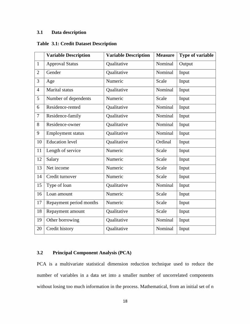
3.1 Data description
Table 3.1: Credit Dataset Description
Variable Description Variable Description Measure Type of variable
1 Approval Status Qualitative Nominal Output
2 Gender Qualitative Nominal Input
3 Age Numeric Scale Input
4 Marital status Qualitative Nominal Input
5 Number of dependents Numeric Scale Input
6 Residence-rented Qualitative Nominal Input
7 Residence-family Qualitative Nominal Input
8 Residence-owner Qualitative Nominal Input
9 Employment status Qualitative Nominal Input
10 Education level Qualitative Ordinal Input
11 Length of service Numeric Scale Input
12 Salary Numeric Scale Input
13 Net income Numeric Scale Input
14 Credit turnover Numeric Scale Input
15 Type of loan Qualitative Nominal Input
16 Loan amount Numeric Scale Input
17 Repayment period months Numeric Scale Input
18 Repayment amount Qualitative Scale Input
19 Other borrowing Qualitative Nominal Input
20 Credit history Qualitative Nominal Input
3.2 Principal Component Analysis (PCA)
PCA is a multivariate statistical dimension reduction technique used to reduce the
number of variables in a data set into a smaller number of uncorrelated components
without losing too much information in the process. Mathematical, from an initial set of n
Page 29
19
correlated variables, PCA creates uncorrelated indices or components, where each
component is a linear weighted combination of the initial variables. The technique
achieves this by creating a fewer number of variables which explain most of the variation
in the original variables. The new variables created are linear combinations of the original
variables.
The uncorrelated property of the components is highlighted by the fact that they are
orthogonal to each other, which mean the indices are measuring different dimensions in
the data (Manly 1994). The weights for each principal component are given by the
eigenvectors of the correlation matrix, or if the original data were standardized, the co-
variance matrix. The variance ( ) for each principal component is given by the
eigenvalue of the corresponding eigenvector. The components are ordered such that the
first component (PC1) explains the largest possible amount of variation in the original
data, subject to the constraint that the sum of the squared weights (2
11a +2
12a + …….. +2
1na
) is equal to one. The eigenvalues equals to the number of variables in the initial data set.
In addition, the proportion of the total variation in the original data set accounted by each
principal component is given by i /n. The second component (PC2) is completely
uncorrelated with the first component, and explains additional but less variation than the
first component, subject to the same constraint, Vyas et al (2006).
Consequently, Vyas et al (2006) cites that, the components are uncorrelated with previous
components; therefore, each component captures an additional dimension in the data set,
while explaining smaller and smaller proportions of the variation of the original
Page 30
20
variables. The higher the degree of correlation among the original variables in the data,
the fewer components required to capture common information.
When using PCA, it is hoped that the eigenvalues of most of the PCs will be so low as to
be virtually negligible. Where this is the case, the variation in the data set can be
adequately described by means of a few PCs where the eigenvalues are not negligible.
3.2.1 Basic assumptions (PCA)
o Multiple variables measured at the continuous level.
o Linear relationship between all variables.
o Sampling adequacy.
o Suitable data for reduction with adequate correlations between the variables.
o No significant outliers.
3.2.2 Summary of PCA approach
a) Getting the whole dataset consisting of p-dimensional samples ignoring the class
labels
pp xaxaxaY 111111 .......
pp xaxaxaY 212122 .......
(1)
pppppp xaxaxaY .......11
Page 31
21
b) Compute the mean vector
c) Standardizing the data
d) Compute the covariance matrix
e) Compute eigenvectors and corresponding eigenvalues
f) Sort the eigenvectors by decreasing eigenvalues
g) Use eigenvector matrix to transform the samples onto the new subspace.
If we do not standardize the data, we can run the analysis also by using the correlation
matrix instead of the covariance matrix. The variance of the data along the principal
component directions is associated with the magnitude of the eigenvalues. The choice of
how many components to extract geometrically is based on the scree plot. This is a useful
visual aid which shows the amount of variance explained by each consecutive
eigenvalue. The choice of how many components to extract is fairly arbitrary. When
conducting principal components analysis prior to further analyses, it is risky to choose
too small a number of components, which may fail to explain enough of the variability in
the data.
3.3 Binary Logistic Regression
Binary Logistic regression or Logit deals with the binary case. It is a special type of
regression where binary response variable is related to a set of explanatory variables that
can be discrete and/or continuous. The model is mostly used to identify the relationship
between two or more explanatory variables iX and the dependent variableY . It has been
used for prediction and determining the most influential explanatory variables on the
dependent variable (Cox and Snell, 1994). The Logistic regression model for the
Page 32
22
dependence of Pi (response probability) on the values of n explanatory variables1X ,
2X ….
nX (Collett, 2003).
P1
Plog) P(
i
iiLogit = nnXX ........110 (2)
Or )........exp(1
)........exp(
110
110
nn
nni
XX
XXP
. (3)
This is linear and similar to the expression of multiple linear regressions.
Here,
i
i
P1
P is the ratio of the probability of a failure and called odds 0 , si ' are
parameters to be estimated and iP is the response probability.
We use maximum likelihood method (MLM) to estimate si ' , which maximizes the
probability of getting the observed results given the fitted regression coefficients.
);()/(1
i
n
i
ii yfyL
Likelihood function, where iy take a binomial distribution. We
estimate the model coefficients as a function )(ˆii y . The predicted response values
will lies between 0 and 1 regardless of the values of the explanatory variables.
3.3.1 Basic assumptions of Binary Logistic Regression
o LR does not assume a linear relationship between the dependent and independent
variables.
o The dependent variable must be binary.
o The independent variables need not be interval, nor normally distributed, nor linearly
related, nor of equal variance within each group.
Page 33
23
o Little or no multicollinearity
o The categories must be mutually exclusive and exhaustive.
o Large samples sizes are required ( at least 50)
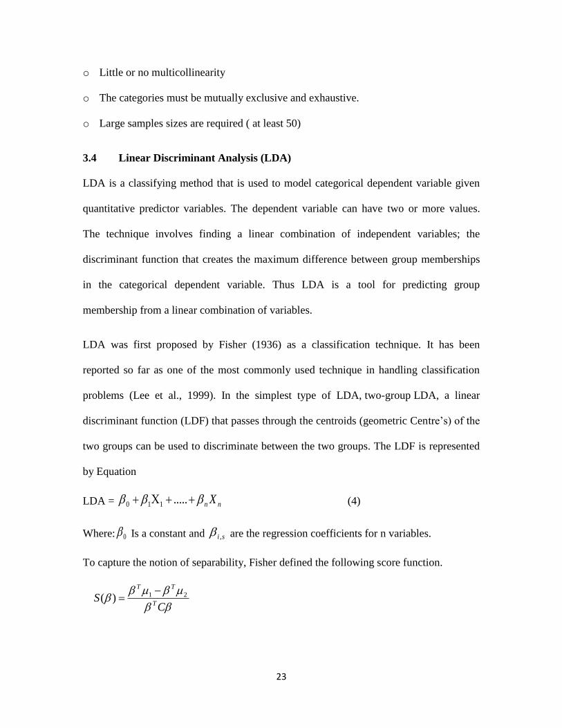
3.4 Linear Discriminant Analysis (LDA)
LDA is a classifying method that is used to model categorical dependent variable given
quantitative predictor variables. The dependent variable can have two or more values.
The technique involves finding a linear combination of independent variables; the
discriminant function that creates the maximum difference between group memberships
in the categorical dependent variable. Thus LDA is a tool for predicting group
membership from a linear combination of variables.
LDA was first proposed by Fisher (1936) as a classification technique. It has been
reported so far as one of the most commonly used technique in handling classification
problems (Lee et al., 1999). In the simplest type of LDA, two-group LDA, a linear
discriminant function (LDF) that passes through the centroids (geometric Centre’s) of the
two groups can be used to discriminate between the two groups. The LDF is represented
by Equation
LDA = nn X .....110 (4)
Where: 0 Is a constant and si , are the regression coefficients for n variables.
To capture the notion of separability, Fisher defined the following score function.
CS
T
TT
21)(
Page 34
24
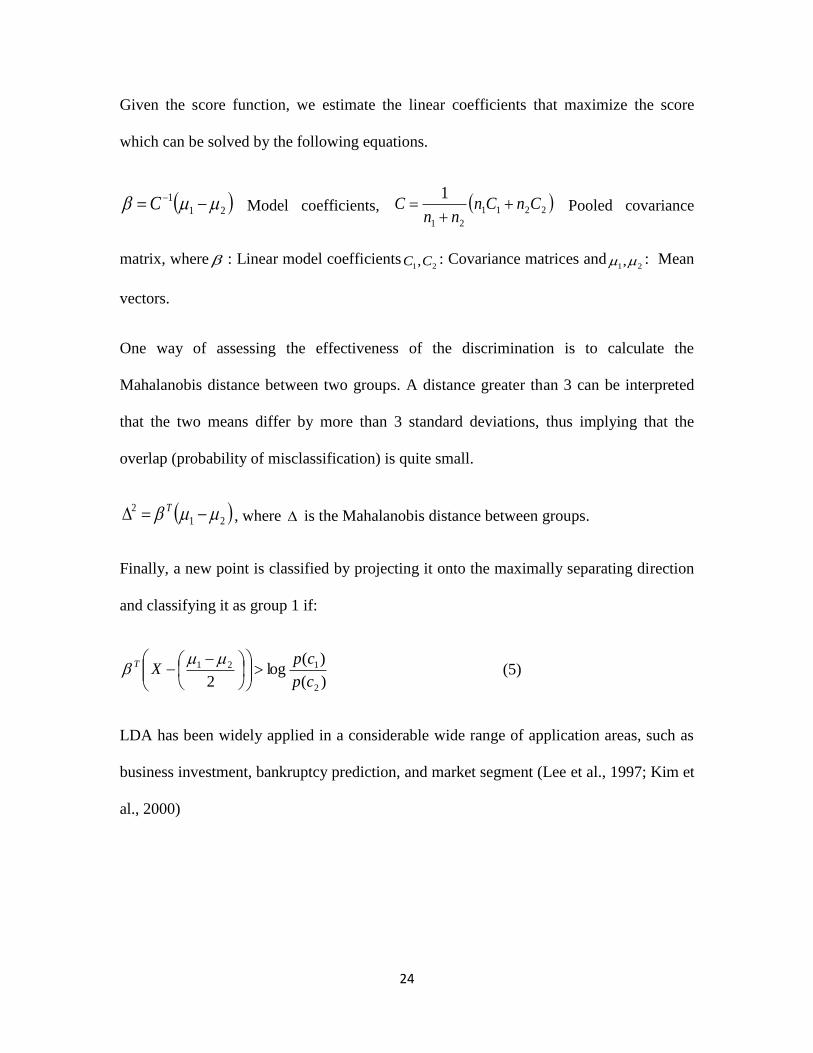
Given the score function, we estimate the linear coefficients that maximize the score
which can be solved by the following equations.
21
1 C Model coefficients, 2211
21
1CnCn
nnC
Pooled covariance
matrix, where : Linear model coefficients21,CC : Covariance matrices and
21, : Mean
vectors.
One way of assessing the effectiveness of the discrimination is to calculate the
Mahalanobis distance between two groups. A distance greater than 3 can be interpreted
that the two means differ by more than 3 standard deviations, thus implying that the
overlap (probability of misclassification) is quite small.
21
2 T, where is the Mahalanobis distance between groups.
Finally, a new point is classified by projecting it onto the maximally separating direction
and classifying it as group 1 if:
)(
)(log
2 2
121
cp
cpXT
(5)
LDA has been widely applied in a considerable wide range of application areas, such as
business investment, bankruptcy prediction, and market segment (Lee et al., 1997; Kim et
al., 2000)
Page 35
25
3.4.1 Basic assumptions (LDA)
The analysis is quite sensitive to outliers and the size of the smallest group must be larger
than the number of predictor variables. The assumptions include:-
o Multivariate normality: each predictor variable is normally distributed.
o Homoscedasticity: Variances among group variables are the same across levels of
predictors.
o Little or no multicollinearity
o Independence: The observations are a random sample.
o At least two groups or categories, with each case belonging to only one group so that
the groups are mutually exclusive and collectively exhaustive.
Each group or category must be well defined, clearly differentiated from any other
group(s). The groups or categories should be defined before collecting the data; the
attribute(s) used to separate the groups should discriminate quite clearly between the
groups so that group or category overlap is clearly non-existent or minimal; group sizes
of the dependent should not be grossly different and should be at least five times the
number of independent variables. It has been suggested that discriminant analysis is
relatively robust to slight violations of these assumptions, and it has also been shown that
discriminant analysis may still be reliable when using dichotomous variables (where
multivariate normality is often violated).
Page 36
26
3.4.2 Summary the LDA approach
In this approach we Calculate the:
o Mean vectors.
o Covariance matrices.
o Class probabilities.
o Pooled covariance matrix
o Coefficients of the linear model.
3.5 Hypothesis testing
3.5.1 KMO and Bartlett’s test
Test Statistics: KMO. In this case the following hypothesis is tested.
1H : The sampled data is adequate for the study
aH1 : The sampled data is not adequate for the study.
Decision Rule: We reject 1H at =0.05 level of significance if p-value < 0.05.
Otherwise we fail to reject 1H and conclude that the sampled data is adequate for the
study.
Bartlett’s test
In this case the following hypothesis is tested.
2H : 1 =
2 = ……………………..= k
aH 2 : ji For at least one pair ( i , j )
Page 37
27
Decision Rule: We reject 2H at =0.05 level of significance if p-value < 0.05.
Otherwise we fail to reject 2H and conclude that the sample variances across variables
for Credit scoring are not equal
3.5.2 Wilks’ Lambda Test for significance of canonical correlation:
In this case the following hypothesis is tested.
3H : There is no linear relationship between the credit status (output variables) and the
input variables in the LR model
aH3 : There is linear is a relationship between the credit status (output variables) and the
input variables in the LR model
Test statistic:
HW
W
, where W is residual variance, H is the variance due to linear relationship
and (W+H) is the total variance.
Decision Rule: We reject 3H at =0.05 level of significance if p-value < 0.05.
Otherwise we fail to reject 3H and conclude that there is no linear relationship between
the credit status (output variables) and the input variables in the LR model
Page 38
28
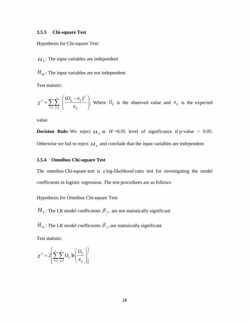
3.5.3 Chi-square Test
Hypothesis for Chi-square Test:
4H : The input variables are independent
aH 4 : The input variables are not independent
Test statistic:
ij
ijijr
i
c
j e
eO 2
1 1
2)(
, Where ijO is the observed value and ije is the expected
value.
Decision Rule: We reject 4H at =0.05 level of significance if p-value < 0.05.
Otherwise we fail to reject 4H and conclude that the input variables are independent
3.5.4 Omnibus Chi-square Test
The omnibus Chi-square test is a log-likelihood ratio test for investigating the model
coefficients in logistic regression. The test procedures are as follows:
Hypothesis for Omnibus Chi-square Test:
5H : The LR model coefficients sj ' are not statistically significant
aH5 : The LR model coefficients sj ' are statistically significant
Test statistic:
r
i ij
ijc
j
ije
OO
1 1
2 ln2
Page 39
29
Decision Rule: We reject 5H at =0.05 level of significance if p-value < 0.05.
Otherwise we fail to reject 5H and conclude that the LR model coefficients sj ' are not
statistically significant
3.5.5 Box M Test for the Equality of Covariance Matrices
Hypothesis for Box’s M Test:
6H : The two covariance matrices are equal for the creditworthy and non-creditworthy
groups in the LDA model
aH 6 : The two covariance matrices are not equal for the creditworthy and non-
creditworthy groups in the LDA model
Test Statistic:
S
L
S
SM , Where
LS is the larger variance and SS is the smaller variance.
Decision Rule: We fail to reject 6H at =0.05 level of significance if p-value < 0.05.
Otherwise we reject 6H and conclude that the two covariance matrices are equal for the
creditworthy and non-creditworthy groups in the LDA model
3.5.6 Wald Test
The Wald test is used to test the statistical significance of each coefficient ( j ) in the
logistic model.
7H : 0j
aH 7 : 0j
Page 40
30
Test Statistic:
SEW
This value is squared which yields a chi- square distribution and is used as a Wald test
statistics.
Decision Rule: We reject 7H : at =0.05 level of significance if p-value < 0.05.
Otherwise we fail to reject 7H : and conclude that the sampled data is adequate for the
study
Page 41
31
CHAPTER FOUR
DATA ANALYSIS AND RESULTS
4.1 Introduction
In this chapter, various tests were conducted that helped in data analysis and obtaining
the results. The results are then interpreted.
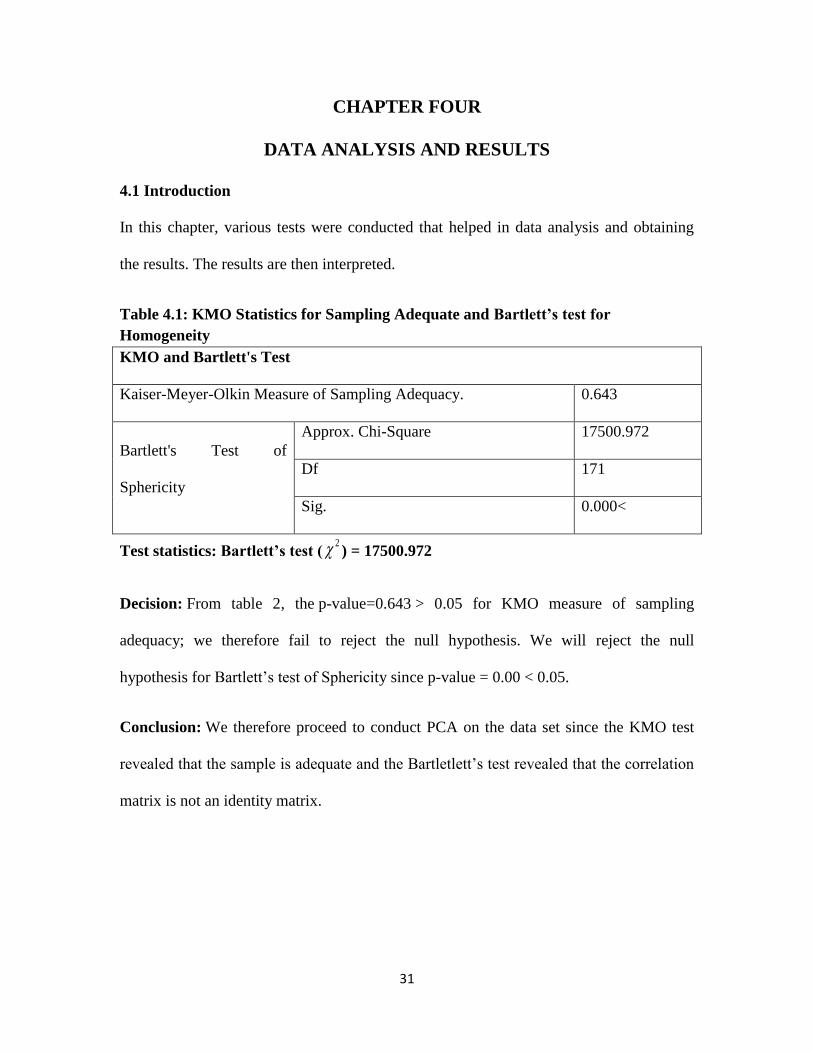
Table 4.1: KMO Statistics for Sampling Adequate and Bartlett’s test for
Homogeneity
KMO and Bartlett's Test
Kaiser-Meyer-Olkin Measure of Sampling Adequacy. 0.643
Bartlett's Test of
Sphericity
Approx. Chi-Square 17500.972
Df 171
Sig. 0.000<
Test statistics: Bartlett’s test (2 ) = 17500.972
Decision: From table 2, the p-value=0.643 > 0.05 for KMO measure of sampling
adequacy; we therefore fail to reject the null hypothesis. We will reject the null
hypothesis for Bartlett’s test of Sphericity since p-value = 0.00 < 0.05.
Conclusion: We therefore proceed to conduct PCA on the data set since the KMO test
revealed that the sample is adequate and the Bartletlett’s test revealed that the correlation
matrix is not an identity matrix.
Page 42
32
4.2 PCA output
Table 4.2: PCA Total Variance Explained
Component
Initial Eigenvalues Extraction Sums of Squared
Loadings
Total % of
Variance
Cumulative
% Total
% of
Variance
Cumulative
%
Dimension
1 5.545 29.185 29.185 5.545 29.185 29.185
2 2.675 14.08 43.265 2.675 14.08 43.265
3 1.542 8.117 51.381 1.542 8.117 51.381
4 1.292 6.797 58.179 1.292 6.797 58.179
5 1.233 6.49 64.669 1.233 6.49 64.669
6 1.111 5.845 70.514 1.111 5.845 70.514
7 1.059 5.572 76.086 1.059 5.572 76.086
8 0.995 5.236 81.321
9 0.932 4.905 86.226
10 0.839 4.414 90.64
11 0.688 3.622 94.262
12 0.416 2.19 96.452
13 0.241 1.267 97.718
14 0.199 1.045 98.763
15 0.106 0.559 99.322
16 0.065 0.342 99.664
17 0.031 0.162 99.826
18 0.024 0.124 99.95
19 0.01 0.05 100
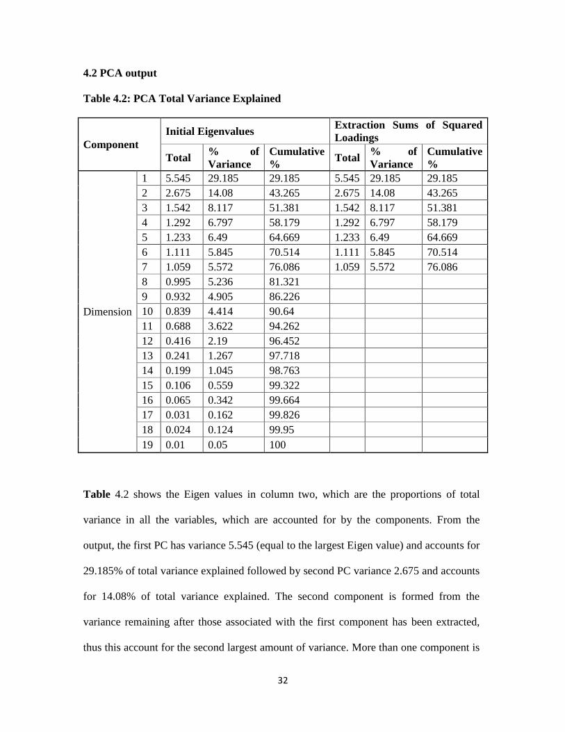
Table 4.2 shows the Eigen values in column two, which are the proportions of total
variance in all the variables, which are accounted for by the components. From the
output, the first PC has variance 5.545 (equal to the largest Eigen value) and accounts for
29.185% of total variance explained followed by second PC variance 2.675 and accounts
for 14.08% of total variance explained. The second component is formed from the
variance remaining after those associated with the first component has been extracted,
thus this account for the second largest amount of variance. More than one component is
Page 43
33
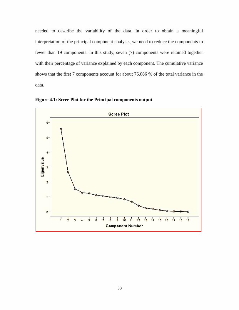
needed to describe the variability of the data. In order to obtain a meaningful
interpretation of the principal component analysis, we need to reduce the components to
fewer than 19 components. In this study, seven (7) components were retained together
with their percentage of variance explained by each component. The cumulative variance
shows that the first 7 components account for about 76.086 % of the total variance in the
data.
Figure 4.1: Scree Plot for the Principal components output
Page 44
34
Table 4.3: The Coefficient of Principal Component Score of Variables
Component Matrix
Variable Name Component
1 2 3 4 5 6 7
Gender .074 -.009 -.172 .014 .091 -.047 .268
Age .685 .636 -.036 -.010 -.086 .151 .010
Marital Status .315 .435 -.046 .055 -.061 .435 .078
Number Dependent’s .588 .641 .012 .031 -.013 .184 -.027
Residence-Rented -.005 -.231 -.909 .121 .075 .242 .017
Residence-Family -.277 -.317 .718 -.034 -.259 .423 .075
Residence-Owner .285 .573 .214 -.066 .228 -.645 -.103
Employment Status -.028 -.012 .092 -.053 -.052 -.001 .821
Education Level .608 -.501 .093 -.031 .263 .013 -.008
Length of Service .601 .666 -.036 -.046 -.223 .117 .088
Salary .896 -.241 .074 -.071 .136 .044 -.011
Net Income .892 -.339 .002 -.128 -.051 -.027 -.011
Credit Turnover .854 -.401 -.007 -.158 -.095 -.052 .003
Type of Loan .041 .010 -.010 .239 .575 .069 .280
Amount .753 -.237 .080 .498 -.115 -.095 -.024
Repayment Period .049 -.050 .044 .901 -.335 -.167 .028
Repayment Amount .912 -.269 .046 -.073 .052 .018 -.017
Other Borrowing -.073 .053 .146 .181 .319 .368 -.433
Credit History -.040 .163 .257 .245 .614 .114 .119
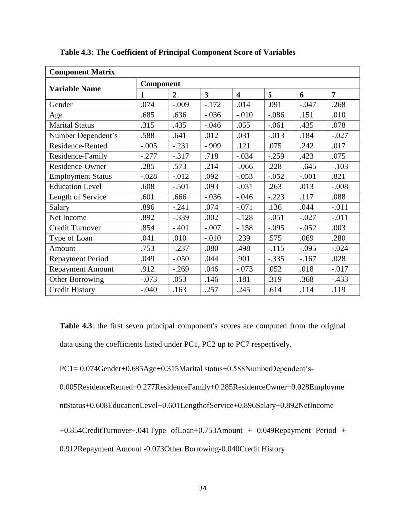
Table 4.3: the first seven principal component's scores are computed from the original
data using the coefficients listed under PC1, PC2 up to PC7 respectively.
PC1= 0.074Gender+0.685Age+0.315Marital status+0.588NumberDependent’s-
0.005ResidenceRented+0.277ResidenceFamily+0.285ResidenceOwner+0.028Employme
ntStatus+0.608EducationLevel+0.601LengthofService+0.896Salary+0.892NetIncome
+0.854CreditTurnover+.041Type ofLoan+0.753Amount + 0.049Repayment Period +
0.912Repayment Amount -0.073Other Borrowing-0.040Credit History
Page 45
35
.
.
PC7.
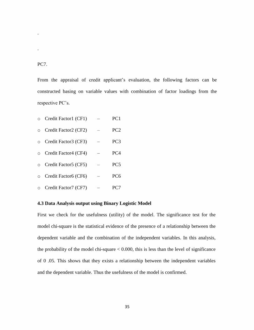
From the appraisal of credit applicant’s evaluation, the following factors can be
constructed basing on variable values with combination of factor loadings from the
respective PC’s.
o Credit Factor1 (CF1) – PC1
o Credit Factor2 (CF2) – PC2
o Credit Factor3 (CF3) – PC3
o Credit Factor4 (CF4) – PC4
o Credit Factor5 (CF5) – PC5
o Credit Factor6 (CF6) – PC6
o Credit Factor7 (CF7) – PC7
4.3 Data Analysis output using Binary Logistic Model
First we check for the usefulness (utility) of the model. The significance test for the
model chi-square is the statistical evidence of the presence of a relationship between the
dependent variable and the combination of the independent variables. In this analysis,
the probability of the model chi-square < 0.000, this is less than the level of significance
of 0 .05. This shows that they exists a relationship between the independent variables
and the dependent variable. Thus the usefulness of the model is confirmed.
Page 46
36
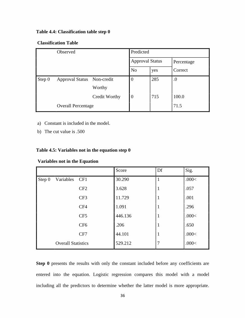
Table 4.4: Classification table step 0
Classification Table
Observed Predicted
Approval Status Percentage
Correct No yes
Step 0 Approval Status Non-credit
Worthy
0 285 .0
Credit Worthy 0 715 100.0
Overall Percentage 71.5
a) Constant is included in the model.
b) The cut value is .500
Table 4.5: Variables not in the equation step 0
Variables not in the Equation
Score Df Sig.
Step 0 Variables CF1 30.290 1 .000<
CF2 3.628 1 .057
CF3 11.729 1 .001
CF4 1.091 1 .296
CF5 446.136 1 .000<
CF6 .206 1 .650
CF7 44.101 1 .000<
Overall Statistics 529.212 7 .000<
Step 0 presents the results with only the constant included before any coefficients are
entered into the equation. Logistic regression compares this model with a model
including all the predictors to determine whether the latter model is more appropriate.
Page 47
37
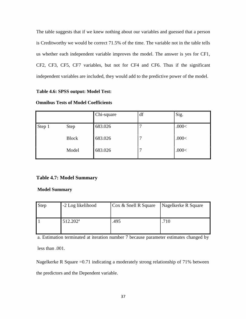
The table suggests that if we knew nothing about our variables and guessed that a person
is Creditworthy we would be correct 71.5% of the time. The variable not in the table tells
us whether each independent variable improves the model. The answer is yes for CF1,
CF2, CF3, CF5, CF7 variables, but not for CF4 and CF6. Thus if the significant
independent variables are included, they would add to the predictive power of the model.
Table 4.6: SPSS output: Model Test:
Omnibus Tests of Model Coefficients
Chi-square df Sig.
Step 1 Step 683.026 7 .000<
Block 683.026 7 .000<
Model 683.026 7 .000<
Table 4.7: Model Summary
Model Summary
Step -2 Log likelihood Cox & Snell R Square Nagelkerke R Square
1 512.202a .495 .710
a. Estimation terminated at iteration number 7 because parameter estimates changed by
less than .001.
Nagelkerke R Square =0.71 indicating a moderately strong relationship of 71% between
the predictors and the Dependent variable.
Page 48
38
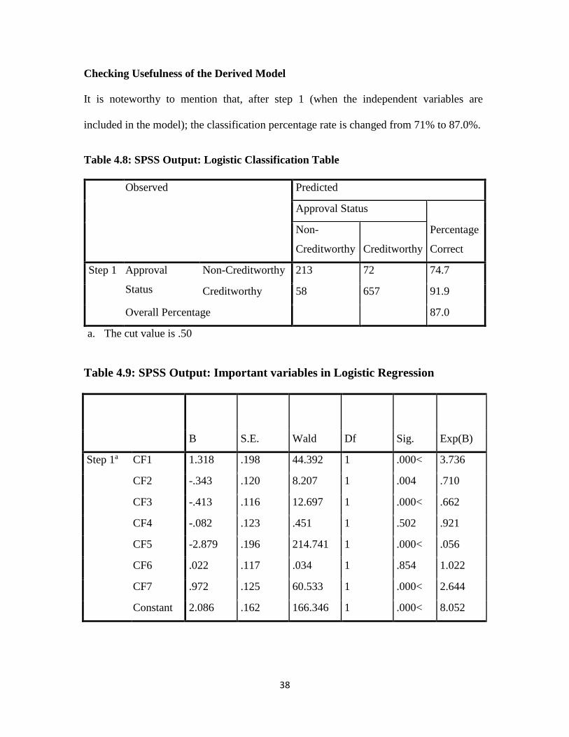
Checking Usefulness of the Derived Model
It is noteworthy to mention that, after step 1 (when the independent variables are
included in the model); the classification percentage rate is changed from 71% to 87.0%.
Table 4.8: SPSS Output: Logistic Classification Table
Observed Predicted
Approval Status
Percentage
Correct
Non-
Creditworthy Creditworthy
Step 1 Approval
Status
Non-Creditworthy 213 72 74.7
Creditworthy 58 657 91.9
Overall Percentage 87.0
a. The cut value is .50
Table 4.9: SPSS Output: Important variables in Logistic Regression
B S.E. Wald Df Sig. Exp(B)
Step 1a CF1 1.318 .198 44.392 1 .000< 3.736
CF2 -.343 .120 8.207 1 .004 .710
CF3 -.413 .116 12.697 1 .000< .662
CF4 -.082 .123 .451 1 .502 .921
CF5 -2.879 .196 214.741 1 .000< .056
CF6 .022 .117 .034 1 .854 1.022
CF7 .972 .125 60.533 1 .000< 2.644
Constant 2.086 .162 166.346 1 .000< 8.052
Page 49
39
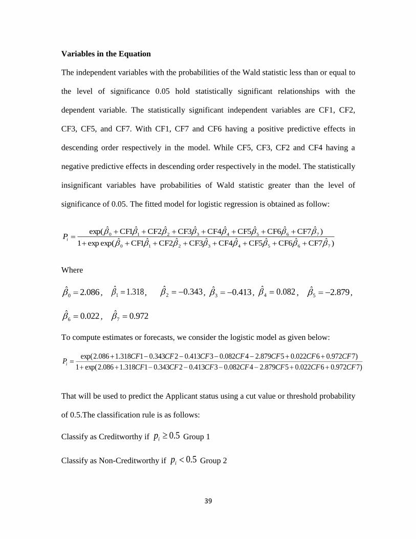
Variables in the Equation
The independent variables with the probabilities of the Wald statistic less than or equal to
the level of significance 0.05 hold statistically significant relationships with the
dependent variable. The statistically significant independent variables are CF1, CF2,
CF3, CF5, and CF7. With CF1, CF7 and CF6 having a positive predictive effects in
descending order respectively in the model. While CF5, CF3, CF2 and CF4 having a
negative predictive effects in descending order respectively in the model. The statistically
insignificant variables have probabilities of Wald statistic greater than the level of
significance of 0.05. The fitted model for logistic regression is obtained as follow:
)ˆ7CFˆ6CFˆ5CFˆ4CFˆ3CFˆ2CFˆ1CFˆexp(exp1
)ˆ7CFˆ6CFˆ5CFˆ4CFˆ3CFˆ2CFˆ1CFˆexp(
76543210
76543210
iP
Where
086.2ˆ0 , 318.1ˆ
1 , 343.0ˆ2 , 413.0ˆ
3 , 082.0ˆ4 , 879.2ˆ
5 ,
022.0ˆ6 , 972.0ˆ
7
To compute estimates or forecasts, we consider the logistic model as given below:
)7972.06022.05879.24082.03413.02343.01318.1086.2exp(1
)7972.06022.05879.24082.03413.02343.01318.1086.2exp(
CFCFCFCFCFCFCF
CFCFCFCFCFCFCFPi
That will be used to predict the Applicant status using a cut value or threshold probability
of 0.5.The classification rule is as follows:
Classify as Creditworthy if 5.0ip Group 1
Classify as Non-Creditworthy if 5.0ip Group 2
Page 50
40
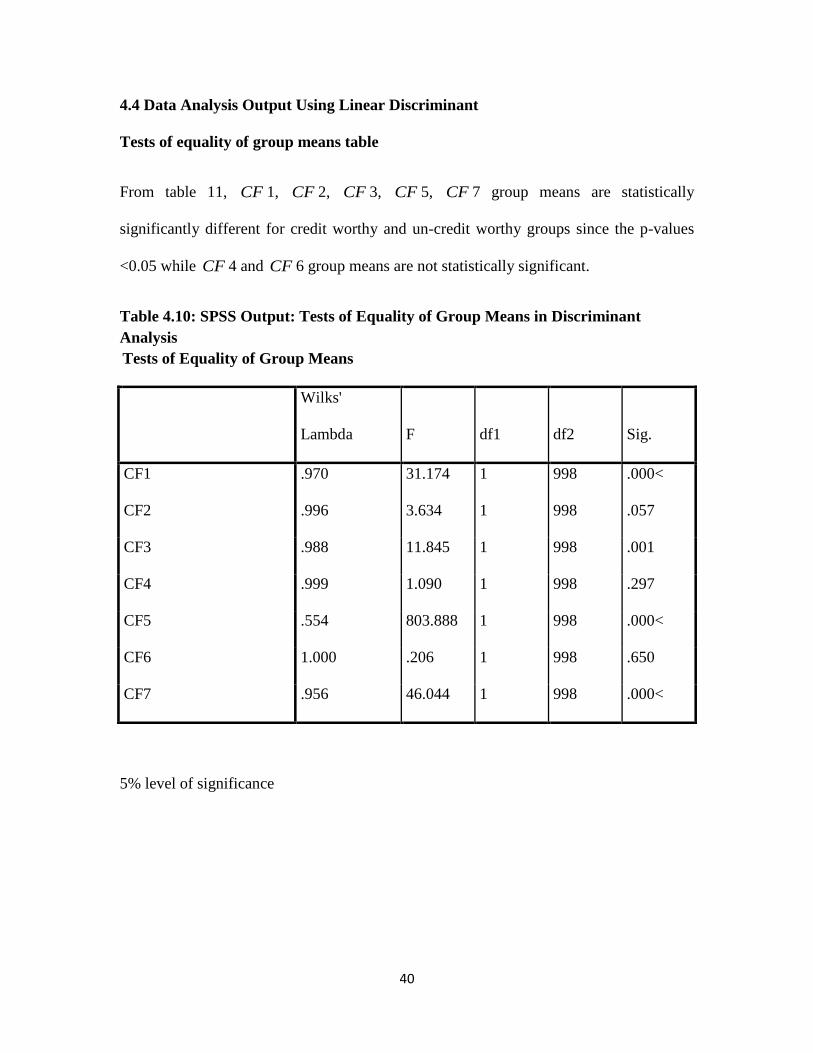
4.4 Data Analysis Output Using Linear Discriminant
Tests of equality of group means table
From table 11, CF 1, CF 2, CF 3, CF 5, CF 7 group means are statistically
significantly different for credit worthy and un-credit worthy groups since the p-values
<0.05 while CF 4 and CF 6 group means are not statistically significant.
Table 4.10: SPSS Output: Tests of Equality of Group Means in Discriminant
Analysis
Tests of Equality of Group Means
Wilks'
Lambda F df1 df2 Sig.
CF1 .970 31.174 1 998 .000<
CF2 .996 3.634 1 998 .057
CF3 .988 11.845 1 998 .001
CF4 .999 1.090 1 998 .297
CF5 .554 803.888 1 998 .000<
CF6 1.000 .206 1 998 .650
CF7 .956 46.044 1 998 .000<
5% level of significance
Page 51
41
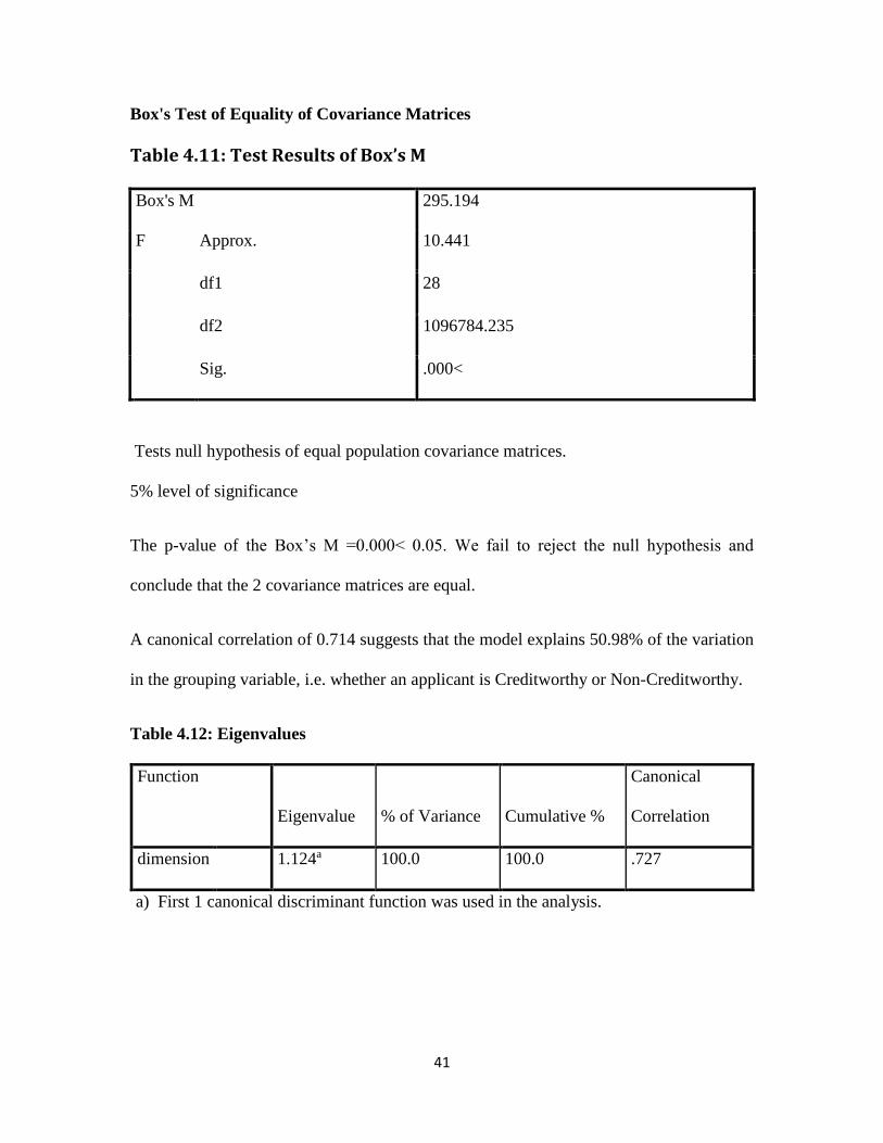
Box's Test of Equality of Covariance Matrices
Table 4.11: Test Results of Box’s M
Box's M 295.194
F Approx. 10.441
df1 28
df2 1096784.235
Sig. .000<
Tests null hypothesis of equal population covariance matrices.
5% level of significance
The p-value of the Box’s M =0.000< 0.05. We fail to reject the null hypothesis and
conclude that the 2 covariance matrices are equal.
A canonical correlation of 0.714 suggests that the model explains 50.98% of the variation
in the grouping variable, i.e. whether an applicant is Creditworthy or Non-Creditworthy.
Table 4.12: Eigenvalues
Function
Eigenvalue % of Variance Cumulative %
Canonical
Correlation
dimension 1.124a 100.0 100.0 .727
a) First 1 canonical discriminant function was used in the analysis.
Page 52
42
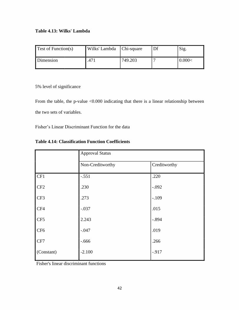
Table 4.13: Wilks' Lambda
Test of Function(s) Wilks' Lambda Chi-square Df Sig.
Dimension .471 749.203 7 0.000<
5% level of significance
From the table, the p-value <0.000 indicating that there is a linear relationship between
the two sets of variables.
Fisher’s Linear Discriminant Function for the data
Table 4.14: Classification Function Coefficients
Approval Status
Non-Creditworthy Creditworthy
CF1 -.551 .220
CF2 .230 -.092
CF3 .273 -.109
CF4 -.037 .015
CF5 2.243 -.894
CF6 -.047 .019
CF7 -.666 .266
(Constant) -2.100 -.917
Fisher's linear discriminant functions
Page 53
43
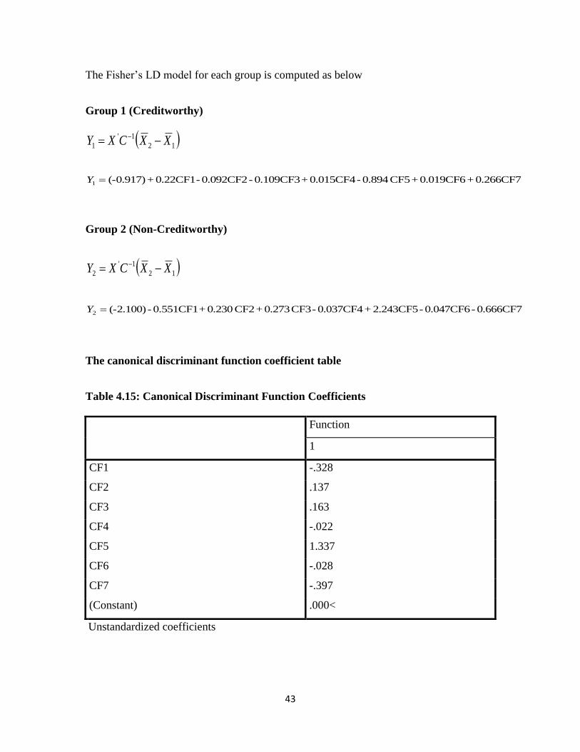
The Fisher’s LD model for each group is computed as below
Group 1 (Creditworthy)
12
1'
1 XXCXY
0.266CF7 +0.019CF6 +CF5 0.894-0.015CF4+0.109CF3-0.092CF2-0.22CF1 +(-0.917)1 Y
Group 2 (Non-Creditworthy)
12
1'
2 XXCXY
0.666CF7 - 0.047CF6 -2.243CF5 +0.037CF4-CF3 0.273 +CF2 0.230 +0.551CF1- (-2.100)2 Y
The canonical discriminant function coefficient table
Table 4.15: Canonical Discriminant Function Coefficients
Function
1
CF1 -.328
CF2 .137
CF3 .163
CF4 -.022
CF5 1.337
CF6 -.028
CF7 -.397
(Constant) .000<
Unstandardized coefficients
Page 54
44
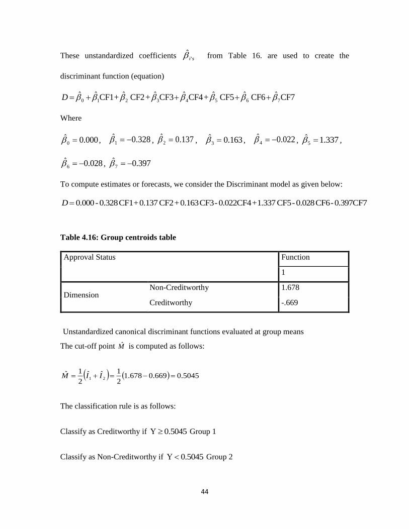
These unstandardized coefficients si '̂ from Table 16. are used to create the
discriminant function (equation)
CF7ˆ CF6 ˆ CF5 ˆ+CF4ˆ CF3ˆ+CF2 ˆ+CF1ˆˆ76543210 D
Where
000.0ˆ0 , 328.0ˆ
1 , 137.0ˆ2 , 163.0ˆ
3 , 022.0ˆ4 , 337.1ˆ
5 ,
028.0ˆ6 , 397.0ˆ
7
To compute estimates or forecasts, we consider the Discriminant model as given below:
0.397CF7-CF6 0.028 - CF5 1.337+0.022CF4 - CF3 0.163+CF2 0.137+CF1 0.328 - 0.000D
Table 4.16: Group centroids table
Approval Status Function
1
Dimension Non-Creditworthy 1.678
Creditworthy -.669
Unstandardized canonical discriminant functions evaluated at group means
The cut-off point M̂ is computed as follows:
5045.0669.0678.12
1ˆˆ2
1ˆ21 IIM
The classification rule is as follows:
Classify as Creditworthy if 5045.0 Group 1
Classify as Non-Creditworthy if 5045.0 Group 2
Page 55
45
Table 4.17: Prior Probabilities for Groups
Approval Status
Prior
Cases Used in Analysis
Unweighted Weighted
Non-Creditworthy .500 285 285.000
Creditworthy .500 715 715.000
Total 1.000 1000 1000.000
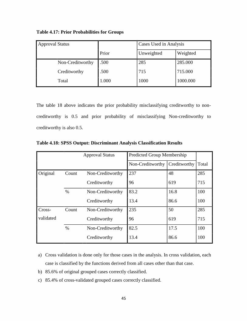
The table 18 above indicates the prior probability misclassifying creditworthy to non-
creditworthy is 0.5 and prior probability of misclassifying Non-creditworthy to
creditworthy is also 0.5.
Table 4.18: SPSS Output: Discriminant Analysis Classification Results
Approval Status Predicted Group Membership
Total Non-Creditworthy Creditworthy
Original Count
Non-Creditworthy 237 48 285
Creditworthy 96 619 715
%
Non-Creditworthy 83.2 16.8 100
Creditworthy 13.4 86.6 100
Cross-
validated
Count
Non-Creditworthy 235 50 285
Creditworthy 96 619 715
%
Non-Creditworthy 82.5 17.5 100
Creditworthy 13.4 86.6 100
a) Cross validation is done only for those cases in the analysis. In cross validation, each
case is classified by the functions derived from all cases other than that case.
b) 85.6% of original grouped cases correctly classified.
c) 85.4% of cross-validated grouped cases correctly classified.
Page 56
46
Classification Results:
Predictive Ability of the Discriminant Model
From the above table, the Discriminant model is able to classify 619 good applicants as
“Good Group” out of 715 good applicants. Thus, it holds 86.6% classification accuracy
for the good group. On the other hand, the same discriminant model is able to classify
237 bad applicants as “Bad Group” out of 285 bad applicants. Thus, it holds 83.2%
classification accuracy for the bad group. As a result, the model is able to generate 85.6%
classification accuracy in combined groups.
Page 57
47
CHAPTER FIVE
CONCLUSIONS AND RECOMMEDATIONS
5.1 Introduction
This project described the process by which large dimensional data sets with independent
variables being highly correlated can be addressed by performing PCA on the data before
employing the analysis using either Logistic or Discriminant models to Classify credit
applicants. The main advantage for the use of PCA is that it’s computationally easier and
uses all the variables in reducing the dimensionality. In this case, 7 uncorrelated PC’s
were retained reducing the predictor variables used in the analysis from 19 to 7.
The choice of variables to be included in the model is one of the key factors for success
or failure of credit scoring model performance. Although credit scoring assessment is one
of the most successful applications of applied statistics, the best statistical models do not
promise credit scoring success, it normally depends on the; experienced risk management
practices, the way models are developed and applied, and proper use of the management
information systems (Mays 1998).
The Discriminant model and Binary Logistic regression were used to classify applicant
status using the credit scores obtained from credit factors (CF) for previous credit
applicants. Using the credit scores from the CF obtained as weights, a dependent variable
is constructed for each of the applicants having a mean zero and standard deviation equal
to one. This dependent variable for the new credit applicant is regarded to as a credit
score, in our case, p̂ in logistic regression model and D̂ in Discriminant analysis model.
These scores are used against set up cut-off criteria explained below. The higher the score
Page 58
48
the more creditworthy the applicant is and the lower the score the less creditworthy the
applicant is.
The credit scores are predicted from continuous independent variables in the Logistic and
Discriminant models, though the estimated coefficient may not be easy to interpret. In
this project for prediction, we used cut-off points to differentiate credit applicants into
two categories; creditworthy and un-creditworthy. In the Logistic model the cut-off point
is set as 0.5 and in the discriminant model the cut off point was obtain in the analysis as
0.5045. Applicants below this cut-off points are considered to as un-creditworthy and
those equal to or greater than as creditworthy.
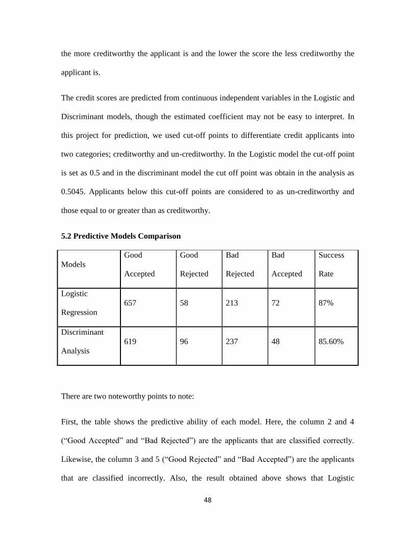
5.2 Predictive Models Comparison
Models
Good
Accepted
Good
Rejected
Bad
Rejected
Bad
Accepted
Success
Rate
Logistic
Regression
657 58 213 72 87%
Discriminant
Analysis
619 96 237 48 85.60%
There are two noteworthy points to note:
First, the table shows the predictive ability of each model. Here, the column 2 and 4
(“Good Accepted” and “Bad Rejected”) are the applicants that are classified correctly.
Likewise, the column 3 and 5 (“Good Rejected” and “Bad Accepted”) are the applicants
that are classified incorrectly. Also, the result obtained above shows that Logistic
Page 59
49
Regression with a success rate of 87% gave slightly better results than Discriminant
Analysis model with 85.60% for the sample data used. It should be noted that it is not
possible to draw a general conclusion that Logistic regression holds better predictive
ability than Discriminant Analysis because this study covers only one dataset. On the
other hand, statistical models can be used to further explore the nature of the relationship
between the dependent and each independent variable.
Secondly, the table gives an idea about the cost of misclassification which assumed that a
“Bad Accepted” generates much higher costs than a “Good Rejected”, because there is a
chance to lose the whole amount of credit while accepting a “Bad” and only losing the
interest payments while rejecting a “Good”. In this analysis, it is apparent that
Discriminant Analysis with 48 misclassified as creditworthy acquired less amount of
“Bad Accepted” than Logistic regression with 72 misclassified as creditworthy. So,
discriminant analysis achieves less cost of misclassification.
5.3 Discussion
Seema Vyas et al (2006) use the first Principal component in constructing social-
economic status indices. We used 7 PC’s obtained from PCA. Principal component 5 had
the highest effect on the response variable. This implies that large variation alone does
not have the same effect on the overall model.
Suleiman et al (2014) found out that the classification accuracy of DA was 80% while LR
91%. In this project DA 85.6% and LR 87% classification accuracy slightly not different
from Suleiman et al (2014).
Page 60
50
Although credit risk assessment is one of the most successful applications of applied
statistics, the best statistical models do not promise credit scoring success, it depends on
the experienced risk management practices, the way models are developed and applied
and proper use of the management information systems (Mays 1998).
Hand & Henley (1997) found out that there is no best method. They commented that the
best method depends largely on the structure and characteristics of the data. For a data
set, one method may be better than the other method but for another data set, the other
method may be better. Therefore, one has to explore the data characteristics and structure
before adopting any of these models.
5.4 Recommendations
Future Research
Recommend ranking of the importance of variables used in building the scoring models
are almost totally neglected in published research papers on credit scoring. This has
important implications for the policies of the lending institutions system as a whole.
Future research might usefully be employed in investigating this more.
In addition, address and identify drivers of default from a behavioral perspective, and the
impact of trends in; rising costs of living, interest rates and inflation on credit appraisal.
Future studies should aim at using other advanced statistical scoring techniques, such as
genetic algorithms, besides the neural nets and traditional scoring models, and perhaps
integrated with other techniques, such as fuzzy discriminant analysis. Collect more data
and employ more variables that might increase the accuracies of the scoring models
probably use more than one bank’s data-set.
Page 61
51
Incorporated into the modelling procedures time series aspects, so that trends in variable
impact can be predicted. This is especially important for loans of longer duration, whose
default is likely to be associated with differing attributes from those of short loans in a
rapidly changing economic and social environment.
Financial Institutions
Adopt and automate these statistical models in their system for quicker and faster credit
appraisal, charge higher interest for applicants that are most likely to default payment.
The institutions should strive to ensure better data collection and management methods
are put in place. This forms a strong basis for better performance of models and risk
management.
Consider charging different interest rates to customers depending on the credit score
instead of basing on the product line offered. Customers with higher credit scores should
be consider for charging low interest rates while those with low credit scores charging
high interest rates.
Finally, consider integrating statistical modeling and credit score predictions and
classification and other methods as a great tool for credit risk management.
Page 62
52
REFERENCES
Abdou, H.A. and Pointon, J. (2011). Credit Scoring, Statistical Techniques and
Evaluation Criteria: A review of the Literature. Intelligent Systems in Accounting,
Finance and Management 18(2–3): 59–88.
Abdou, H. (2009a). Credit Scoring Models for Egyptian Banks: Neural Nets and Genetic
Programming versus Conventional Techniques, Ph.D. Thesis, The University of
Plymouth, UK.
Abdou, H. (2009b). An Evaluation of Alternative Scoring Models in Private Banking.
Journal of Risk Finance 10 (1): 38-53.
Abdou, H. and Pointon, J. (2011) ‘Credit Scoring, Statistical Techniques and Evaluation
Criteria: A Review of the Literature’. Intelligent systems in accounting, Financial
and Management, 18 (2-3), pp. 59-88
Adnan, K.. (2010). Neural Networks for Credit Risk Evaluation: Investigation of
Different Neural Models and Learning Schemes. Expert Systems with
Applications.
Altman, E.I. (1968). Financial Ratios, Discriminant Analysis and the Prediction of
Corporate Bankruptcy. Journal of Finance 23(4): 589–611.
Altman, E.I. (1968). Financial Ratio Discriminant Analysis and the Prediction of
Corporate Bankruptcy. The Journal of Finance, 23(4), pp. 589-609.
Angelini, E. et al. (2008). The Quarterly Review of Economics and Finance 48 733–755
Antonio Blanco, Rafael Pino-Mejias, Juan Lara, Salvador Rayo, “Credit Scoring models
for MFI using Neural Networks: Evidence from Peru”, Expert Systems with
applications, Vol.40, pp 356-364, 2013.
Colquitt, J. (2007). Credit Risk Management. McGraw-Hill.
Grablowsky, J. B. (1975). A Behavioral Risk in Consumer Credit. The Journal of
Finance, 30(3), 915-916. http://dx.doi.org/10.2307/2326880
Page 63
53
Hand, D. J., Henley, W. E. (1997). Statistical Classification Methods in Consumer Credit
Scoring: A Review. Journal of the Royal Statistical Society: Series A (Statistics in
Society) 160 (3): 523-541.
Jagric, T. & Jagric, V. (2011). A Comparison of Growing Cell Structures Neural
Networks and Linear Scoring Models in the Retail Credit Environment, Eastern
European Economics, vol. 49, no. 6, pg. 74-96
Kleimeier, S. and Dinh, T. (2007). A credit Scoring Model for Vietnam's Retail Banking
Market. International Review of Financial Analysis, 16(5), pp 471{495.
Koh, H.C.& Tan, W.C. and Goh, C.P. (2006): A Two-step Method to construct Credit
Scoring Models with Data Mining Techniques. International Journal of Business
and Information
Kumar, GP.(2007). Hybrid Credit Scoring Algorithm using PCA and SVM.
Lee, T. S., Chiu, C. C., Lu, C. J., & Chen, I. F. (2002). Credit Scoring Using the Hybrid
Neural Discriminant Technique. Expert Systems with Applications, 23(3), 245–
254.
Malhorta, R.. And Malhorta D.K., (2003). Evaluating Consumer Loans Using Neural
Networks: Elsevier Science Ltd.
Martin, D., 1977. Early Warning of Bank Failure: A Logit Regression Approach. Journal
of Banking and Finance 249-276.
Paliwal, M. & Kumar, U. A. (2009). Neural Networks and Statistical Techniques: A
Review of Applications. Expert Systems with Applications 36 (1): 2-17.
Seema, V. and Lilani, K (2006). Constructing Socio-Economic Status Indices: How to
Use Principal Component Analysis. Health Policy Plan, Oxford University press,
21(6):459-68.
Suleiman, S. Issa, Suleiman, U. Usman (2014). Predicting an Applicant Status Using
Principal Component, Discriminant and Logistic Regression Analysis.
Page 64
54
International Journal of Mathematics and Statistics Invention (IJMSI), 2(10),
pp.05-15.
West, D. (2000). Neural Network Credit Scoring Models. Computers & Operations
Research 27(11–12): 1131–1152.
Wiginton, J. C.(1980). A Note on the Comparison of Logit and Discriminant Models of
Consumer Credit 38 Behavior, The Journal of Financial and Quantitative
Analysis, Vol. 15, No. 3, pp. 757-770.
Yao, P. (2009). Hybrid Fuzzy SVM Model Using CART and MARS for Credit Scoring.
In: Proceedings of the International Conference on Intelligent Human-Machine
Systems and Cybernetics, Vol. 2, Hangzhou, China, pp 392–395.
Zhang, D, Hifi M, Chen Q and Ye W (2008a). A hybrid Credit Scoring Model Based on
Genetic Programming and Support Vector Machines. In: Proceedings of the 4th
International Conference on Natural Computation, Washington, USA, pp 8–12.