2nd Symposium on Advances in Approximate Bayesian Inference, 2019 1–12 Approximate Inference for Fully Bayesian Gaussian Process Regression Vidhi Lalchand [email protected]University of Cambridge, Cambridge, UK The Alan Turing Institute, London, UK Carl Edward Rasmussen [email protected]University of Cambridge, Cambridge, UK Abstract Learning in Gaussian Process models occurs through the adaptation of hyperparameters of the mean and the covariance function. The classical approach entails maximizing the marginal likelihood yielding fixed point estimates (an approach called Type II maximum likelihood or ML-II). An alternative learning procedure is to infer the posterior over hyper- parameters in a hierarchical specification of GPs we call Fully Bayesian Gaussian Process Regression (GPR). This work considers two approximation schemes for the intractable hy- perparameter posterior: 1) Hamiltonian Monte Carlo (HMC) yielding a sampling based approximation and 2) Variational Inference (VI) where the posterior over hyperparameters is approximated by a factorized Gaussian (mean-field) or a full-rank Gaussian accounting for correlations between hyperparameters. We analyse the predictive performance for fully Bayesian GPR on a range of benchmark data sets. 1. Motivation The Gaussian process (GP) posterior is heavily influenced by the choice of the covariance function which needs to be set a priori. Specification of a covariance function and setting the hyperparameters of the chosen covariance family are jointly referred to as the model selection problem (Rasmussen and Williams, 2004). A preponderance of literature on GPs address model selection through maximization of the marginal likelihood, ML-II (MacKay, 1999). This is an attractive approach as the marginal likelihood is tractable in the case of a Gaussian noise model. Once the point estimate hyperparameters have been selected typically using conjugate gradient methods the posterior distribution over latent function values and hence predictions can be derived in closed form; a compelling property of GP models. While straightforward to implement the non-convexity of the marginal likelihood surface can pose significant challenges for ML-II. The presence of multiple modes can make the process prone to overfitting especially when there are many hyperparameters. Further, weakly identified hyperparameters can manifest in flat ridges in the marginal likelihood surface (where different combinations of hyperparameters give similar marginal likelihood value) (Warnes and Ripley, 1987) making gradient based optimisation extremely sensitive c V. Lalchand & C.E. Rasmussen.
Transcript
2nd Symposium on Advances in Approximate Bayesian Inference, 2019 1–12
Approximate Inference for Fully Bayesian Gaussian ProcessRegression
Learning in Gaussian Process models occurs through the adaptation of hyperparametersof the mean and the covariance function. The classical approach entails maximizing themarginal likelihood yielding fixed point estimates (an approach called Type II maximumlikelihood or ML-II). An alternative learning procedure is to infer the posterior over hyper-parameters in a hierarchical specification of GPs we call Fully Bayesian Gaussian ProcessRegression (GPR). This work considers two approximation schemes for the intractable hy-perparameter posterior: 1) Hamiltonian Monte Carlo (HMC) yielding a sampling basedapproximation and 2) Variational Inference (VI) where the posterior over hyperparametersis approximated by a factorized Gaussian (mean-field) or a full-rank Gaussian accountingfor correlations between hyperparameters. We analyse the predictive performance for fullyBayesian GPR on a range of benchmark data sets.
1. Motivation
The Gaussian process (GP) posterior is heavily influenced by the choice of the covariancefunction which needs to be set a priori. Specification of a covariance function and settingthe hyperparameters of the chosen covariance family are jointly referred to as the modelselection problem (Rasmussen and Williams, 2004). A preponderance of literature on GPsaddress model selection through maximization of the marginal likelihood, ML-II (MacKay,1999). This is an attractive approach as the marginal likelihood is tractable in the caseof a Gaussian noise model. Once the point estimate hyperparameters have been selectedtypically using conjugate gradient methods the posterior distribution over latent functionvalues and hence predictions can be derived in closed form; a compelling property of GPmodels.
While straightforward to implement the non-convexity of the marginal likelihood surfacecan pose significant challenges for ML-II. The presence of multiple modes can make theprocess prone to overfitting especially when there are many hyperparameters. Further,weakly identified hyperparameters can manifest in flat ridges in the marginal likelihoodsurface (where different combinations of hyperparameters give similar marginal likelihoodvalue) (Warnes and Ripley, 1987) making gradient based optimisation extremely sensitive
to starting values. Overall, the ML-II point estimates for the hyperparameters are subjectto high variability and underestimate prediction uncertainty.
The central challenge in extending the Bayesian treatment to hyperparameters in a hierar-chical framework is that their posterior is highly intractable; this also renders the predictiveposterior intractable. The latter is typically handled numerically by Monte Carlo integra-tion yielding a non-Gaussian predictive posterior; it yields in fact a mixture of GPs. Thekey question about quantifying uncertainty around covariance hyperparameters is exam-ining how this effect propagates to the posterior predictive distribution under differentapproximation schemes.
2. Fully Bayesian GPR
Given observations (X,y) = {xi, yi}Ni=1 where yi are noisy realizations of some latent func-tion values f corrupted with Gaussian noise, yi = fi + εi, εi ∈ N (0, σ2n), let kθ(xi, xj)denote a positive definite covariance function parameterized with hyperparameters θ andthe corresponding covariance matrix Kθ. The hierarchical GP framework is given by,
Prior over hyperparameters θ ∼ p(θ)
Prior over parameters f |X,θ ∼ N (0,Kθ)
Data likelihood y|f ∼ N (f , σ2nI)(1)
The generative model in (1) implies the joint posterior over unknowns given as,
p(f ,θ|y) =1
Zp(y|f)p(f |θ)p(θ) (2)
where Z is the unknown normalization constant. The predictive distribution for unknowntest inputs X? integrates over the joint posterior,
p(f?|y) =
∫ ∫p(f?|f ,θ)p(f ,θ|y)dfdθ (3)
=
∫ ∫p(f?|f ,θ)p(f |θ,y)p(θ|y)dfdθ (4)
(where we have suppressed the conditioning over inputs X,X? for brevity). The innerintegral
∫p(f?|f ,θ)p(f |θ,y)df reduces to the standard GP predictive posterior with fixed
hyperparameters,
p(f?|y,θ) = N (µ?,Σ?)
where,
µ? = K?θ (Kθ + σ2nI)−1y Σ? = K??
θ −K?θ (Kθ + σ2nI)−1K?T
θ (5)
where K??θ denotes the covariance matrix evaluated between the test inputs X? and K∗θ
denotes the covariance matrix evaluated between the test inputs X? and training inputs X.
2
Approximate Inference in Fully Bayesian GPR
Under a Gaussian noise setting the hierarchical predictive posterior is reduced to,
p(f?|y) =
∫p(f?|y,θ)p(θ|y)dθ ' 1
M
M∑j=1
p(f?|y,θj), θj ∼ p(θ|y) (6)
where f is integrated out analytically and θj are draws from the hyperparameter posterior.The only intractable integral we need to deal with is p(θ|y) ∝ p(y|θ)p(θ) and predictiveposterior follows as per eq. (6). Hence, the hierarchical predictive posterior is a multivariatemixture of Gaussians (Appendix section 6.2).
3. Methods
3.1. Hamiltonian Monte Carlo (HMC)
The distinct advantage of HMC over other MCMC methods is the suppression of the randomwalk behaviour typical of Metropolis and variants. Refer to Neal et al. (2011) for a detailedtutorial. In the experiments we use a self-tuning variant of HMC called the No-U-Turn-Sampler (NUTS) proposed in Hoffman and Gelman (2014) in which the path length isdeterministically adjusted for every iteration. Empirically, NUTS is shown to work as wellas a hand-tuned HMC. By using NUTS we avoid the overhead in determining good valuesfor the step-size (ε) and path length (L). We use an identity mass matrix with 500 warm-upiterations and run 4 chains to detect mode switching which can sometimes adversely affectpredictions. Further, the primary variables are declared as the log of the hyperparameterslog(θ) as this eliminates the positivity constraints that we otherwise we need to accountfor. The computational cost of the HMC scheme is dominated by the need to invert thecovariance matrix Kθ which is O(N3).
3.2. Variational Inference
We largely follow the approach in Kucukelbir et al. (2017). We transform the supportof hyperparameters θ such that they live in the real space RJ where J is the number ofhyperparameters. Let η = g(θ) = log(θ) and we proceed by setting the variational familyto,
p(η|y) ≈ qλmf (η) =
J∏j=1
N (ηj |µj , σ2j )
in the mean-field approximation where λmf = (µ1, . . . , µJ , ν1, . . . , νJ) is the vector of un-constrained variational parameters (log(σ2j ) = νj) which live in R2J . In the full rank ap-proximation the variational family takes the form,
qλfr(η) = N (η|µ,LLT )
where we use the Cholesky factorization of the covariance matrix Σ so that the variationalparameters λfr = (µ,L) are unconstrained in RJ+J(J+1)/2. The variational objective,ELBO is maximised in the transformed η space using stochastic gradient ascent and anyintractable expectations are approximated using monte carlo integration.
where the term |Jg−1(η)| denotes the Jacobian of the inverse transformation g−1(η) = eη =θ. The computation of gradients ∇µL,∇νL,∇LL hinges on automatic differentiation andthe re-parametrization trick (Kingma and Welling (2013)). The computational cost periteration is O(NMJ) where J is the number of hyperparameters and M is the number ofMC samples used in computing stochastic gradients.
4. Experiments
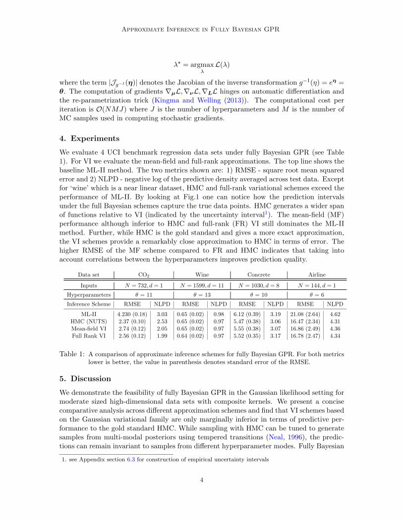
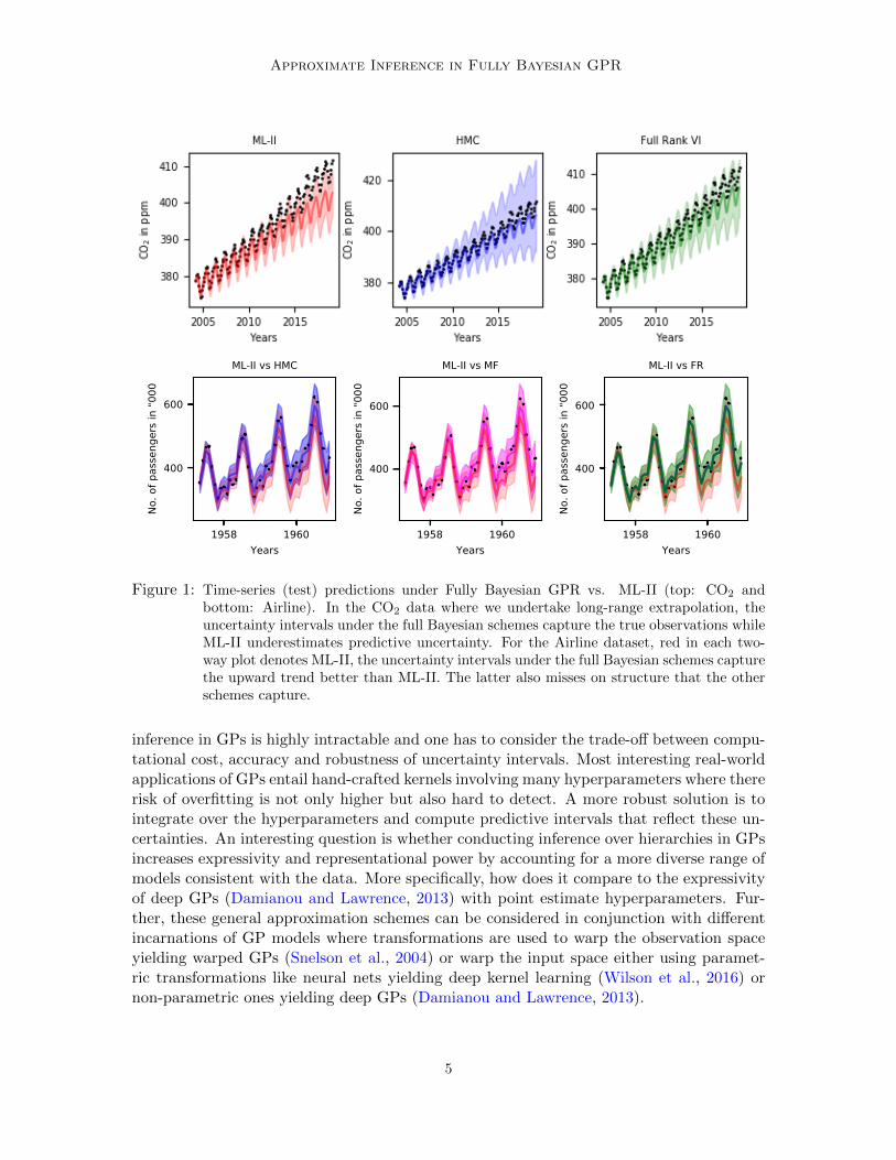
We evaluate 4 UCI benchmark regression data sets under fully Bayesian GPR (see Table1). For VI we evaluate the mean-field and full-rank approximations. The top line shows thebaseline ML-II method. The two metrics shown are: 1) RMSE - square root mean squarederror and 2) NLPD - negative log of the predictive density averaged across test data. Exceptfor ‘wine’ which is a near linear dataset, HMC and full-rank variational schemes exceed theperformance of ML-II. By looking at Fig.1 one can notice how the prediction intervalsunder the full Bayesian schemes capture the true data points. HMC generates a wider spanof functions relative to VI (indicated by the uncertainty interval1). The mean-field (MF)performance although inferior to HMC and full-rank (FR) VI still dominates the ML-IImethod. Further, while HMC is the gold standard and gives a more exact approximation,the VI schemes provide a remarkably close approximation to HMC in terms of error. Thehigher RMSE of the MF scheme compared to FR and HMC indicates that taking intoaccount correlations between the hyperparameters improves prediction quality.
Data set CO2 Wine Concrete Airline
Inputs N = 732, d = 1 N = 1599, d = 11 N = 1030, d = 8 N = 144, d = 1
Table 1: A comparison of approximate inference schemes for fully Bayesian GPR. For both metricslower is better, the value in parenthesis denotes standard error of the RMSE.
5. Discussion
We demonstrate the feasibility of fully Bayesian GPR in the Gaussian likelihood setting formoderate sized high-dimensional data sets with composite kernels. We present a concisecomparative analysis across different approximation schemes and find that VI schemes basedon the Gaussian variational family are only marginally inferior in terms of predictive per-formance to the gold standard HMC. While sampling with HMC can be tuned to generatesamples from multi-modal posteriors using tempered transitions (Neal, 1996), the predic-tions can remain invariant to samples from different hyperparameter modes. Fully Bayesian
1. see Appendix section 6.3 for construction of empirical uncertainty intervals
4
Approximate Inference in Fully Bayesian GPR
1958 1960Years
400
600
No. o
f pas
seng
ers i
n "0
00
ML-II vs HMC
1958 1960Years
400
600
No. o
f pas
seng
ers i
n "0
00
ML-II vs FR
1958 1960Years
400
600
No. o
f pas
seng
ers i
n "0
00ML-II vs MF
Figure 1: Time-series (test) predictions under Fully Bayesian GPR vs. ML-II (top: CO2 andbottom: Airline). In the CO2 data where we undertake long-range extrapolation, theuncertainty intervals under the full Bayesian schemes capture the true observations whileML-II underestimates predictive uncertainty. For the Airline dataset, red in each two-way plot denotes ML-II, the uncertainty intervals under the full Bayesian schemes capturethe upward trend better than ML-II. The latter also misses on structure that the otherschemes capture.
inference in GPs is highly intractable and one has to consider the trade-off between compu-tational cost, accuracy and robustness of uncertainty intervals. Most interesting real-worldapplications of GPs entail hand-crafted kernels involving many hyperparameters where thererisk of overfitting is not only higher but also hard to detect. A more robust solution is tointegrate over the hyperparameters and compute predictive intervals that reflect these un-certainties. An interesting question is whether conducting inference over hierarchies in GPsincreases expressivity and representational power by accounting for a more diverse range ofmodels consistent with the data. More specifically, how does it compare to the expressivityof deep GPs (Damianou and Lawrence, 2013) with point estimate hyperparameters. Fur-ther, these general approximation schemes can be considered in conjunction with differentincarnations of GP models where transformations are used to warp the observation spaceyielding warped GPs (Snelson et al., 2004) or warp the input space either using paramet-ric transformations like neural nets yielding deep kernel learning (Wilson et al., 2016) ornon-parametric ones yielding deep GPs (Damianou and Lawrence, 2013).
5
Approximate Inference in Fully Bayesian GPR
Acknowledgements
VL is funded by The Alan Turing Institute Doctoral Studentship under the EPSRC grantEP/N510129/1.
References
David Barber and Christopher KI Williams. Gaussian processes for bayesian classificationvia hybrid monte carlo. In Advances in neural information processing systems, pages340–346, 1997.
Andreas Damianou and Neil Lawrence. Deep gaussian processes. In Artificial Intelligenceand Statistics, pages 207–215, 2013.
Maurizio Filippone, Mingjun Zhong, and Mark Girolami. A comparative evaluation ofstochastic-based inference methods for gaussian process models. Machine Learning, 93(1):93–114, 2013.
Seth Flaxman, Andrew Gelman, Daniel Neill, Alex Smola, Aki Vehtari, and Andrew GordonWilson. Fast hierarchical gaussian processes. Manuscript in preparation, 2015.
James Hensman, Alexander G Matthews, Maurizio Filippone, and Zoubin Ghahramani.Mcmc for variationally sparse gaussian processes. In Advances in Neural InformationProcessing Systems, pages 1648–1656, 2015.
Matthew D Hoffman and Andrew Gelman. The no-u-turn sampler: adaptively settingpath lengths in hamiltonian monte carlo. Journal of Machine Learning Research, 15(1):1593–1623, 2014.
Diederik P Kingma and Max Welling. Auto-encoding variational bayes. arXiv preprintarXiv:1312.6114, 2013.
Alp Kucukelbir, Dustin Tran, Rajesh Ranganath, Andrew Gelman, and David M Blei. Au-tomatic differentiation variational inference. The Journal of Machine Learning Research,18(1):430–474, 2017.
David JC MacKay. Comparison of approximate methods for handling hyperparameters.Neural computation, 11(5):1035–1068, 1999.
Iain Murray and Ryan P Adams. Slice sampling covariance hyperparameters of latentgaussian models. In Advances in neural information processing systems, pages 1732–1740, 2010.
Radford Neal. Regression and classification using gaussian process priors. Bayesian statis-tics, 6:475, 1998.
Radford M Neal. Sampling from multimodal distributions using tempered transitions.Statistics and computing, 6(4):353–366, 1996.
6
Approximate Inference in Fully Bayesian GPR
Radford M Neal et al. Mcmc using hamiltonian dynamics. Handbook of markov chain montecarlo, 2(11):2, 2011.
Carl Edward Rasmussen and Christopher KI Williams. Gaussian processes in machinelearning. Springer, 2004.
John Salvatier, Thomas V Wiecki, and Christopher Fonnesbeck. Probabilistic programmingin python using pymc3. PeerJ Computer Science, 2:e55, 2016.
Edward Snelson and Zoubin Ghahramani. Sparse gaussian processes using pseudo-inputs.In Advances in neural information processing systems, pages 1257–1264, 2006.
Edward Snelson, Zoubin Ghahramani, and Carl E Rasmussen. Warped gaussian processes.In Advances in neural information processing systems, pages 337–344, 2004.
Michalis Titsias. Variational learning of inducing variables in sparse gaussian processes. InArtificial Intelligence and Statistics, pages 567–574, 2009.
JJ Warnes and BD Ripley. Problems with likelihood estimation of covariance functions ofspatial gaussian processes. Biometrika, 74(3):640–642, 1987.
Christopher KI Williams and Carl Edward Rasmussen. Gaussian processes for regression.In Advances in neural information processing systems, pages 514–520, 1996.
Andrew Gordon Wilson, Zhiting Hu, Ruslan Salakhutdinov, and Eric P Xing. Deep kernellearning. In Artificial Intelligence and Statistics, pages 370–378, 2016.
Haibin Yu, Trong Nghia, Bryan Kian Hsiang Low, and Patrick Jaillet. Stochastic variationalinference for bayesian sparse gaussian process regression. In 2019 International JointConference on Neural Networks (IJCNN), pages 1–8. IEEE, 2019.
6. Appendix
6.1. Related Work
In early accounts, Neal (1998), Williams and Rasmussen (1996) and Barber and Williams(1997) explore the integration over covariance hyperparameters using HMC in the regressionand classification setting. More recently, Murray and Adams (2010) use a slice samplingscheme for covariance hyperparameters in a general likelihood setting specifically address-ing the coupling between latent function values f and hyperparameters θ. Filippone et al.(2013) conduct a comparative evaluation of MCMC schemes for the full Bayesian treatmentof GP models. Other works like Hensman et al. (2015) explore the MCMC approach tovariationally sparse GPs by using a scheme that jointly samples inducing points and hyper-parameters. Flaxman et al. (2015) explore a full Bayesian inference framework for regressionusing HMC but only applies to separable covariance structures together with grid-structuredinputs for scalability. On the variational learning side, Snelson and Ghahramani (2006);Titsias (2009) jointly select inducing points and hyperparameters, hence the posterior overhyperparameters is obtained as a side-effect where the inducing points are the main goal.In more recent work, Yu et al. (2019) propose a novel variational scheme for sparse GPRwhich extends the Bayesian treatment to hyperparameters.
7
Approximate Inference in Fully Bayesian GPR
6.2. First and Second moments of the predictive posterior
The final form of the hierarchical predictive distribution is a multivariate (location-covariance)mixture of Gaussians:
p(f?|y) ' 1
M
M∑j=1
N (µ?θj ,Σ?θj
) (7)
where µ?θj and Σ?θj
denote the GP predictive mean and covariance computed with hyperpa-rameter θj . From standard results on Gaussian mixtures we can derive the first and secondmoments of the hierarchical predictive distribution in (6):
E[f?|y] = µ?m =1
M
M∑j=1
µ?θj E[(f?|y−µ?m)2] =1
M
M∑j=1
Σ?θj
+1
M
M∑j=1
(µ?θj−µ?m)(µ?θj−µ
?m)T
(8)
6.3. Construction of confidence regions
The hierarchical predictive distribution is a mixture of Gaussians and there is no analyticalform for the quantiles of a mixture distribution so we can’t use the predictive variance in(8) per se. We estimate quantiles empirically by simulating samples from the univariatemixture distribution at each test input in X?.
Algorithm 1: 95% Confidence region for the hierarchical predictive distribution
Given: A vector of test inputs X? = (X?1 , . . . , X
?N?)
for each input X?i where i = 1, . . . , N?:
Draw T samples from the univariate mixture distribution
f̂?i ∼ 1M
∑Mj=1N (µ
?(i)θj, σ
?(i)θj
)
Sort the samples in ascending order f̂?i(1) ≤ . . . ≤ f̂?i(T )
Extract the 2.5th percentile ⇒ f?i(rl) where rl =⌈2.5100 × T
⌉Extract the 97.5th percentile ⇒ f?i(ru) where ru =
⌈97.5100 × T
⌉return
f?rl = {f?i(rl)}i=1,...,N?
f?ru = {f?i(ru)}i=1,...,N?
6.4. Kernels and Choice of Priors
All the four data sets use composite kernels constructed from base kernels. Table 2 sum-marizes the base kernels used and the set of hyperparameters for each kernel. All hyperpa-rameters are given vague N (0, 3) priors in log space. Due to the sparsity of Airline data,several of the hyperparameters were weakly identified and in order to constrain inferenceto a reasonable range we resorted to a tighter normal prior around the ML-II estimatesand Gamma(2, 0.1) priors for the noise hyperparameters. All the experiments were done inpython using pymc3 (Salvatier et al., 2016).
8
Approximate Inference in Fully Bayesian GPR
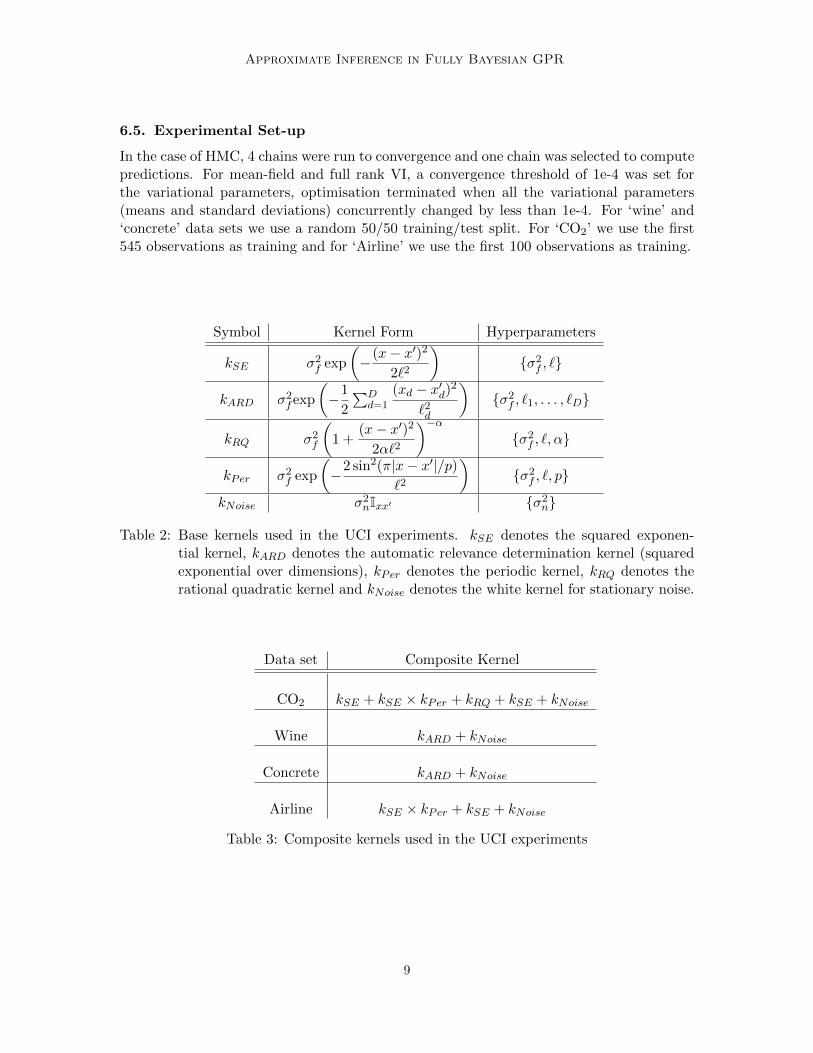
6.5. Experimental Set-up
In the case of HMC, 4 chains were run to convergence and one chain was selected to computepredictions. For mean-field and full rank VI, a convergence threshold of 1e-4 was set forthe variational parameters, optimisation terminated when all the variational parameters(means and standard deviations) concurrently changed by less than 1e-4. For ‘wine’ and‘concrete’ data sets we use a random 50/50 training/test split. For ‘CO2’ we use the first545 observations as training and for ‘Airline’ we use the first 100 observations as training.
Symbol Kernel Form Hyperparameters
kSE σ2f exp
(−(x− x′)2
2`2
){σ2f , `}
kARD σ2fexp
(−1
2
∑Dd=1
(xd − x′d)2
`2d
){σ2f , `1, . . . , `D}
kRQ σ2f
(1 +
(x− x′)2
2α`2
)−α{σ2f , `, α}
kPer σ2f exp
(−2 sin2(π|x− x′|/p)
`2
){σ2f , `, p}
kNoise σ2nIxx′ {σ2n}
Table 2: Base kernels used in the UCI experiments. kSE denotes the squared exponen-tial kernel, kARD denotes the automatic relevance determination kernel (squaredexponential over dimensions), kPer denotes the periodic kernel, kRQ denotes therational quadratic kernel and kNoise denotes the white kernel for stationary noise.
Data set Composite Kernel
CO2 kSE + kSE × kPer + kRQ + kSE + kNoise
Wine kARD + kNoise
Concrete kARD + kNoise
Airline kSE × kPer + kSE + kNoise
Table 3: Composite kernels used in the UCI experiments
9
Approximate Inference in Fully Bayesian GPR
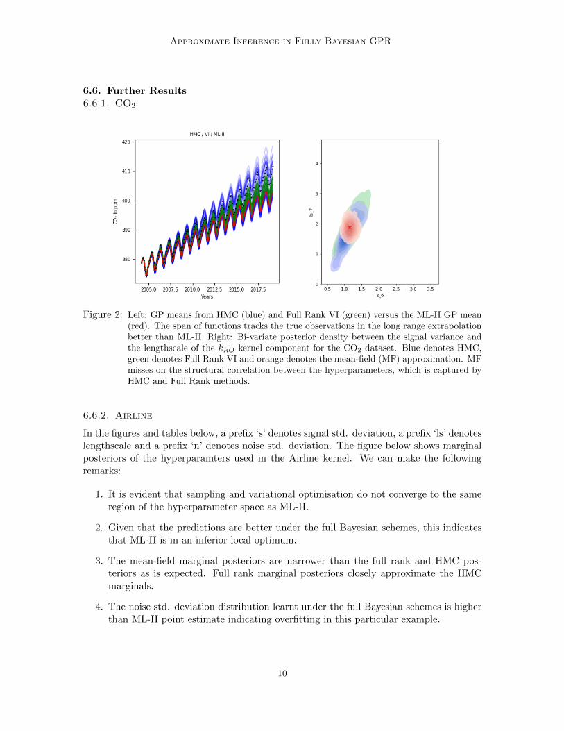
6.6. Further Results
6.6.1. CO2
Figure 2: Left: GP means from HMC (blue) and Full Rank VI (green) versus the ML-II GP mean(red). The span of functions tracks the true observations in the long range extrapolationbetter than ML-II. Right: Bi-variate posterior density between the signal variance andthe lengthscale of the kRQ kernel component for the CO2 dataset. Blue denotes HMC,green denotes Full Rank VI and orange denotes the mean-field (MF) approximation. MFmisses on the structural correlation between the hyperparameters, which is captured byHMC and Full Rank methods.
6.6.2. Airline
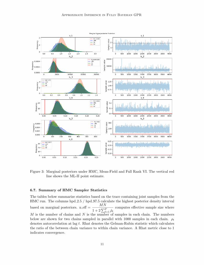
In the figures and tables below, a prefix ‘s’ denotes signal std. deviation, a prefix ‘ls’ denoteslengthscale and a prefix ‘n’ denotes noise std. deviation. The figure below shows marginalposteriors of the hyperparamters used in the Airline kernel. We can make the followingremarks:
1. It is evident that sampling and variational optimisation do not converge to the sameregion of the hyperparameter space as ML-II.
2. Given that the predictions are better under the full Bayesian schemes, this indicatesthat ML-II is in an inferior local optimum.
3. The mean-field marginal posteriors are narrower than the full rank and HMC pos-teriors as is expected. Full rank marginal posteriors closely approximate the HMCmarginals.
4. The noise std. deviation distribution learnt under the full Bayesian schemes is higherthan ML-II point estimate indicating overfitting in this particular example.
10
Approximate Inference in Fully Bayesian GPR
Figure 3: Marginal posteriors under HMC, Mean-Field and Full Rank VI. The vertical redline shows the ML-II point estimate.
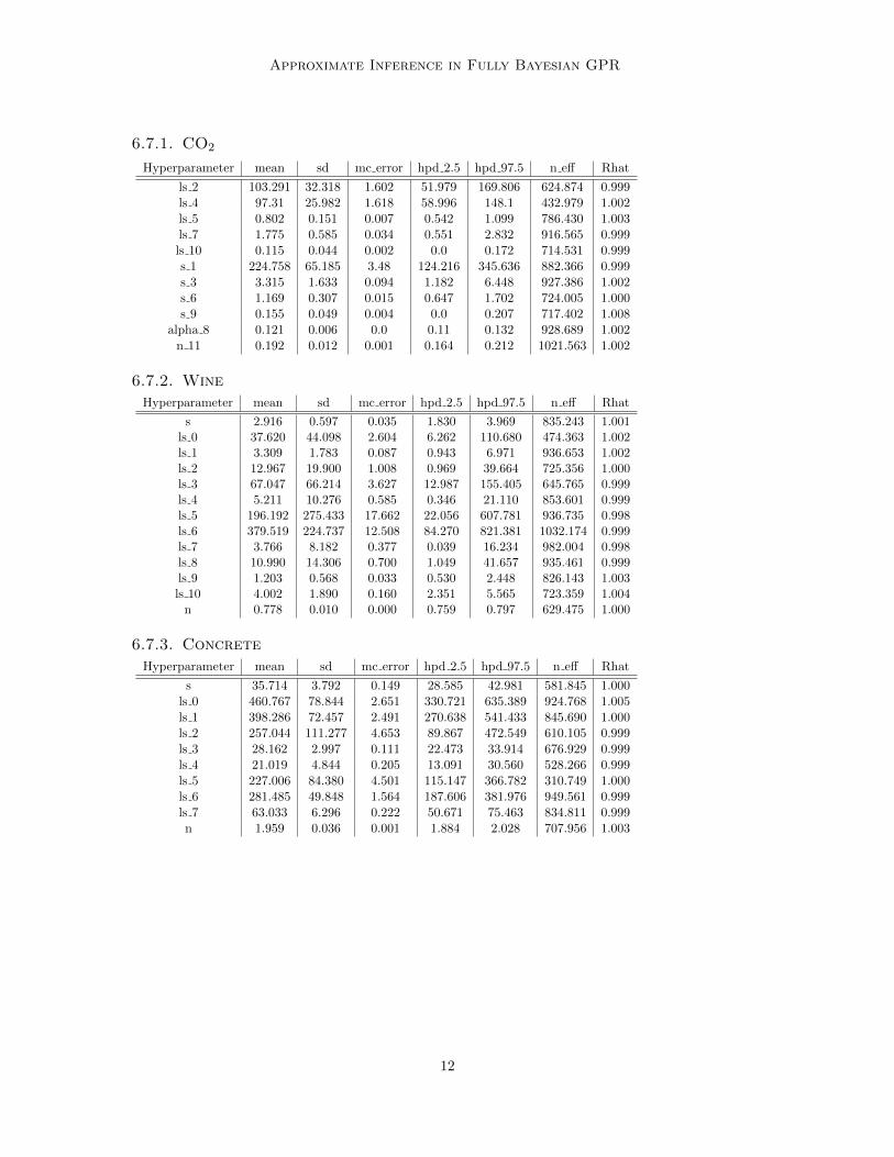
6.7. Summary of HMC Sampler Statistics
The tables below summarize statistics based on the trace containing joint samples from theHMC run. The columns hpd 2.5 / hpd 97.5 calculate the highest posterior density interval
based on marginal posteriors. n eff =MN
1 + 2∑T
t=1 ρ̂tcomputes effective sample size where
M is the number of chains and N is the number of samples in each chain. The numbersbelow are shown for two chains sampled in parallel with 1000 samples in each chain. ρtdenotes autocorrelation at lag t. Rhat denotes the Gelman-Rubin statistic which calculatesthe ratio of the between chain variance to within chain variance. A Rhat metric close to 1indicates convergence.
11
Approximate Inference in Fully Bayesian GPR
6.7.1. CO2
Hyperparameter mean sd mc error hpd 2.5 hpd 97.5 n eff Rhat


![Approximate Inference for Deep Latent Gaussian …enalisni/BDL_paper20.pdf · Approximate Inference for Deep Latent Gaussian Mixtures ... Burda et al. [2] proposed an importance weighted](https://static.documents.pub/doc/80x56/5b68fe837f8b9a6f778d7757/approximate-inference-for-deep-latent-gaussian-enalisnibdl-approximate-inference.jpg)
