416

Approximate inference for the loss-calibrated Bayesian

Simon Lacoste-Julien Ferenc Huszar Zoubin GhahramaniUniversity of Cambridge University of Cambridge University of Cambridge

Abstract

We consider the problem of approximate infer-ence in the context of Bayesian decision theory.Traditional approaches focus on approximat-ing general properties of the posterior, ignor-ing the decision task – and associated losses– for which the posterior could be used. Weargue that this can be suboptimal and pro-pose instead to loss-calibrate the approximateinference methods with respect to the decisiontask at hand. We present a general frameworkrooted in Bayesian decision theory to analyzeapproximate inference from the perspectiveof losses, opening up several research direc-tions. As a first loss-calibrated approximateinference attempt, we propose an EM-like al-gorithm on the Bayesian posterior risk andshow how it can improve a standard approachto Gaussian process classification when lossesare asymmetric.

1 INTRODUCTION

Bayesian methods have enjoyed a surge of popular-ity in machine learning over the last decade. Eventhough it is sometimes overlooked, the main theoreticalmotivations for the Bayesian paradigm are rooted inBayesian decision theory (Berger, 1985), which pro-vides a well-defined theoretical framework for rationaldecision making under uncertainty about a hidden pa-rameter θ. The ingredients of Bayesian decision theoryare an observation model p(D|θ), a prior distributionp(θ), and a loss L(θ, a) for an action a ∈ A. In thisframework, the optimal action is chosen by minimizingits expected loss over the posterior p(θ|D). The inde-pendence of the posterior from the loss motivates thecommon practice of breaking decision making into twoindependent sub-problems: inference, whereby the pos-terior p(θ|D) is computed irrespectively of the loss; and

Appearing in Proceedings of the 14th International Con-ference on Artificial Intelligence and Statistics (AISTATS)2011, Fort Lauderdale, FL, USA. Volume 15 of JMLR:W&CP 15. Copyright 2011 by the authors.

then decision, whereby an action is chosen to minimizeits expected loss over our posterior belief.

In practically interesting Bayesian models, however,the posterior is often computationally intractable andtherefore one has to resort to approximate inferencetechniques, such as variational methods or Markovchain Monte Carlo. Most approaches to approximateinference ignore the decision theoretic loss and try toapproximate the posterior based on its general features,such as matching its mode or higher order moments.While this is probably a reasonable approach for thesimple losses usually considered or when the loss isunknown, they might fail to work well with asymmetric,non-trivial losses that appear in modern applicationsin machine learning.

The main message of the present paper is that wheninference is carried out only approximately, treating(approximate) inference and decision making indepen-dently can lead to suboptimal decisions for a fixed lossunder consideration. We thus investigate whether onecan “calibrate” the approximate inference algorithm toa fixed loss, and propose an analysis framework to an-alyze this situation. We note that a related philosophyhas already been applied in the frequentist discrimina-tive machine learning literature, as for example withthe use of surrogate loss functions (Bartlett et al., 2006;Steinwart and Christmann, 2008). In contrast, we fo-cus in this paper on the pure subjectivist Bayesianviewpoint as we are not yet aware of the existence ofsuch an investigation in this case. The contributionsof the present paper can be summarized as follows:

1. In Sec. 2, we propose a general approximate infer-ence framework based on Bayesian decision theoryto guide our analysis. The framework naturallygives rise to a divergence between distributionsthat can be seen as a loss-calibrated generaliza-tion of the Kullback-Leibler divergence for generallosses. We focus in this paper on the applicationof the framework to the predictive setting that isrelevant to supervised machine learning.

2. In Sec. 3, we present an algorithmic template toderive loss-calibrated approximate inference algo-rithms for different losses by applying the varia-

417

Approximate inference for the loss-calibrated Bayesian

tional Expectation-Maximization algorithm on theBayesian posterior risk.

3. In Sec. 4, we investigate our approximation frame-work on the concrete setup of supervised learning.We apply the loss-calibrated EM algorithm to aGaussian process classification model and analyzeits performance in terms of the loss-calibratedframework. Our proof-of-concept experiments in-dicate that it improves over a loss-insensitive ap-proximate inference alternative and that the ad-vantage of loss-calibration is more prominent whenmisclassification losses are asymmetric.

2 BAYESIAN DECISION THEORY

We use Bayesian statistical decision theory as the basisof our analysis (see Ch. 2 of Robert (2001) or Ch. 1of Berger (1985) for example). We review here its mainingredients:

• a (statistical) loss L(θ, a) which gives the cost oftaking action a ∈ A when the world state is θ ∈ Θ;

• an observation model p(D|θ) which gives the prob-ability of observing D ∈ O assuming that theworld state is θ;

• a prior belief p(θ) over world states.

The loss L describes the decision task that we areinterested in, whereas the observation model and theprior represent our beliefs about the world. Given these,the Bayesian evaluation metric for a possible action aafter observing D is the expected posterior loss (alsocalled the posterior risk (Schervish, 1995)): RpD (a)

.=∫

ΘL(θ, a) p(θ|D)dθ, and so the (Bayes) optimal action

apD is the one that minimizes RpD .

2.1 Supervised learning

We now relate this abstract decision theory setup tothe typical supervised learning applications of machinelearning. For a prediction task, the goal is to estimatea function h : X → Y where the output space Y canbe discrete (classification) or continuous (regression).We suppose that we are given a fixed cost function`(y, y′) which gives the cost of predicting y′ when thetrue output was y. We can cast this problem in thestandard statistical decision theory setting by defining asuitable prediction loss for our action a = h, namely thestandard generalization error from machine learning:

L(θ, h).= E(x,y)∼p(x,y|θ) [` (y, h(x))] . (1)

For the observation model, we will assume that we aregiven a training set D = {(xi, yi)Ni=1} of labeled obser-vations generated i.i.d. from p(x, y|θ). The goal of thelearning algorithm is then to output a function h cho-sen from a set of (possibly non-parametric) hypotheses

H after looking at the (training) data D. From thepure Bayesian point of view, the best hypothesis hpDis clear: it is the one that minimizes the posterior risk,i.e. hpD

.= arg minh∈HRpD (h).

2.2 General approximation framework

The quantity central to the Bayesian methodology isthe posterior pD(θ)

.= p(θ|D) which summarizes our

uncertainty about the world. On the other hand, itis rarely computable in a tractable form, and so it isusually approximated with a tractable approximate dis-tribution q(θ) ∈ Q. Popular approaches to this probleminclude sampling, variational inference – which mini-mizes KL(q‖pD), and expectation propagation – whichminimizes KL(pD‖q) (Minka, 2001). Most approxi-mate inference approaches stop at q, though in thecontext of decision theory, we still need to act. Inpractice, one usually treats the approximate q as ifit was the true posterior and chooses the action thatminimizes what we will call the q-risk :

Rq(h).=

∫Θ

q(θ)L(θ, h)dθ, (2)

obtaining a q-optimal action hq:

hq.= arg min

h∈HRq(h). (3)

In this paper, we will assume that computing exactlythe q-optimal action hq for q ∈ Q is tractable, and focuson the problem of choosing a suitable q to approximatethe posterior pD in order to yield a decision hq withlow posterior risk RpD(hq), mimicking the standardmethodology but crystallizing the decision theoreticgoal. Given this approach, a (usually non-unique) op-timal q ∈ Q is clearly:

qopt = arg minq∈Q

RpD (hq), (4)

though a practical algorithm might only be able to findan approximate minimizer to this quantity. In the casewhere pD ∈ Q, pD is obviously optimal according tothis criterion.

We could interpret the above criterion as minimiz-ing the following asymmetric non-negative discrepancymeasure between distributions:

dL(p‖q) .= Rp(hq)−Rp(hp). (5)

Interestingly, the Kullback-Leibler divergence KL(p‖q)can be interpreted as a special case of dL for the taskof posterior density estimation over Θ. In this task, anaction h is a density over Θ and the standard densityestimation statistical loss is L(θ, h) = − log h(θ). Theq-risk Rq(h) then becomes the cross-entropy H(q, h) =−∫

Θq(θ) log(h(θ))dθ, and so hq = q assuming that

418

Simon Lacoste-Julien, Ferenc Huszar, Zoubin Ghahramani

θ (plant temperature) Tcrit

P[T<θ]

p(θ

)

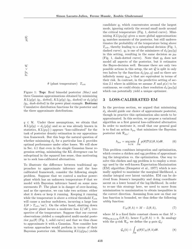
Figure 1: Top: Real bimodal posterior (blue) andthree Gaussian approximations obtained by minimizingKL(q‖p) (q1, dotted), KL(p‖q) (q2, dashed) or dL(p‖q)(q3, dash-dotted) in the power plant example. Bottom:Cumulative distribution functions for the posterior andthe three approximate distributions.

q ∈ H. Under these assumptions, we obtain thatKL(p‖q) = dL(p‖q) and so as was already known instatistics, KL(pD‖·) appears “loss-calibrated” for thetask of posterior density estimation in our approxima-tion framework. But this begs the natural question ofwhether minimizing dL for a particular loss L providesoptimal performance under other losses. We will showin Sec. 4.1 that even in the simple Gaussian linear re-gression setting, minimizing the KL divergence can besuboptimal in the squared loss sense, thus motivatingus to seek loss-calibrated alternatives.

To illustrate the difference between traditional ap-proaches to approximate inference and the loss-calibrated framework, consider the following simpleproblem. Suppose that we control a nuclear power-plant which has an unknown temperature θ that wemodel with Bayesian inference based on some mea-surements D. The plant is in danger of over-heating,and as the operator, we can take two actions: eithershut it down or keep it running. Keeping it runningwhile the temperature is above a critical threshold Tcrit

will cause a nuclear meltdown, incurring a large lossL(θ > Tcrit, ’on’). On the other hand, shutting downthe power plant incurs a moderate loss L(’off’), irre-spective of the temperature. Suppose that our currentobservations yielded a complicated multi-modal poste-rior pD(θ) (Fig. 1, solid curve) and that we thus choseto approximate it with a Gaussian. Now consider howvarious approaches would perform in terms of theirBayesian posterior risk. Minimizing KL(q‖pD) yields

candidate q1 which concentrates around the largestmode, ignoring entirely the second small mode aroundthe critical temperature (Fig. 1, dotted curve). Mini-mizing KL(pD‖q) gives a more global approximation:q2 matches moments of the posterior, but still underes-timates the probability of the temperature being aboveTcrit, thereby leading to a suboptimal decision (Fig. 1,dashed curve). q3 is one of the minimizers of dL(pD‖q)in this setting, resulting in the same decision as pD(Fig. 1, dash-dotted curve). Note that q3 does notmodel all aspects of the posterior, but it estimatesthe Bayes-decision well. Because there are only twopossible actions in this setup, the set Q is split in onlytwo halves by the function dL(pD, q) and so there areinfinitely many qopt’s that are equivalent in terms oftheir risk. In contrast, in the predictive setting of sec-tion 2.1 where in addition we assume X and p(x) to becontinuous, we could obtain a finer resolution dL(pD‖q)which can potentially yield a unique optimizer.

3 LOSS-CALIBRATED EM

In the previous section, we argued that minimizingdL should guide our choice of approximate posterior,though in practice this optimization also needs to beapproximated. In this section, we propose a variationalalgorithm as a first general loss-calibrated alternative.In order to motivate it, recall that our general goalis to find an action hpD that minimizes the Bayesianposterior risk RpD :

hpD = arg minh∈H

∫Θ

p(θ|D)L(θ, h)dθ. (6)

This problem combines integration and optimization,which creates a chicken and egg problem of approximat-ing the integration vs. the optimization. One way tosolve this chicken and egg problem is to employ a strat-egy used by the well-known Expectation-Maximization(EM) algorithm (Dempster et al., 1977) which is nor-mally applied to maximize the marginal likelihood, asimilar integral over latent variables. EM can be de-rived from Jensen’s inequality and doing coordinateascent on a lower bound of the log-likelihood. In orderto re-use this strategy here, we need to move fromminimization to maximization to obtain inequalities inthe correct direction. Assuming from now on that ourloss function is bounded, we thus define the followingutility function:

UM (θ, h).= M − L(θ, h), (7)

where M is a fixed finite constant chosen so that M >supθ∈Θ,h∈H L(θ, h), hence UM (θ, h) > 0. In analogywith the q-risk Rq, we define the q-gain Gq:

Gq(h).=

∫Θ

q(θ)UM (θ, h)dθ. (8)

419

Approximate inference for the loss-calibrated Bayesian

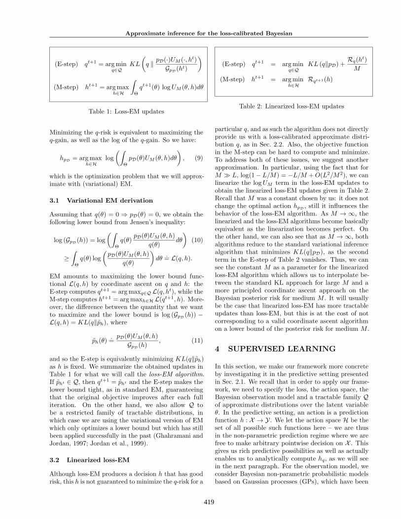
(E-step) qt+1 = arg minq∈Q

KL

(q ‖ pD(·)UM (·, ht)

GpD (ht)

)

(M-step) ht+1 = arg maxh∈H

∫Θ

qt+1(θ) logUM (θ, h)dθ

Table 1: Loss-EM updates

Minimizing the q-risk is equivalent to maximizing theq-gain, as well as the log of the q-gain. So we have:

hpD = arg maxh∈H

log

(∫Θ

pD(θ)UM (θ, h)dθ

), (9)

which is the optimization problem that we will approx-imate with (variational) EM.

3.1 Variational EM derivation

Assuming that q(θ) = 0 ⇒ pD(θ) = 0, we obtain thefollowing lower bound from Jensen’s inequality:

log (GpD (h)) = log

(∫Θ

q(θ)pD(θ)UM (θ, h)

q(θ)dθ

)(10)

≥∫

Θ

q(θ) log

(pD(θ)UM (θ, h)

q(θ)

)dθ

.= L(q, h).

EM amounts to maximizing the lower bound func-tional L(q, h) by coordinate ascent on q and h: theE-step computes qt+1 = arg maxq∈Q L(q, ht), while theM-step computes ht+1 = arg maxh∈H L(qt+1, h). More-over, the difference between the quantity that we wantto maximize and the lower bound is log (GpD (h)) −L(q, h) = KL(q‖ph), where

ph(θ).=pD(θ)UM (θ, h)

GpD (h), (11)

and so the E-step is equivalently minimizing KL(q‖ph)as h is fixed. We summarize the obtained updates inTable 1 for what we will call the loss-EM algorithm.If pht ∈ Q, then qt+1 = pht and the E-step makes thelower bound tight, as in standard EM, guaranteeingthat the original objective improves after each fulliteration. On the other hand, we also allow Q tobe a restricted family of tractable distributions, inwhich case we are using the variational version of EMwhich only optimizes a lower bound but which has stillbeen applied successfully in the past (Ghahramani andJordan, 1997; Jordan et al., 1999).

3.2 Linearized loss-EM

Although loss-EM produces a decision h that has goodrisk, this h is not guaranteed to minimize the q-risk for a

(E-step) qt+1 = arg minq∈Q

KL (q‖pD) +Rq(ht)M

(M-step) ht+1 = arg minh∈H

Rqt+1(h)

Table 2: Linearized loss-EM updates

particular q, and as such the algorithm does not directlyprovide us with a loss-calibrated approximate distri-bution q, as in Sec. 2.2. Also, the objective functionin the M-step can be hard to compute and minimize.To address both of these issues, we suggest anotherapproximation. In particular, using the fact that forM � L, log(1− L/M) = −L/M +O(L2/M2), we canlinearize the logUM term in the loss-EM updates toobtain the linearized loss-EM updates given in Table 2.Recall that M was a constant chosen by us: it does notchange the optimal action hpD , still it influences thebehavior of the loss-EM algorithm. As M → ∞, thelinearized and the loss-EM algorithms become basicallyequivalent as the linearization becomes perfect. Onthe other hand, we can also see that as M →∞, bothalgorithms reduce to the standard variational inferencealgorithm that minimizes KL(q‖pD), as the secondterm in the E-step of Table 2 vanishes. Thus, we cansee the constant M as a parameter for the linearizedloss-EM algorithm which allows us to interpolate be-tween the standard KL approach for large M and amore principled coordinate ascent approach on theBayesian posterior risk for medium M . It will usuallybe the case that linearized loss-EM has more tractableupdates than loss-EM, but this is at the cost of notcorresponding to a valid coordinate ascent algorithmon a lower bound of the posterior risk for medium M .

4 SUPERVISED LEARNING

In this section, we make our framework more concreteby investigating it in the predictive setting presentedin Sec. 2.1. We recall that in order to apply our frame-work, we need to specify the loss, the action space, theBayesian observation model and a tractable family Qof approximate distributions over the latent variableθ. In the predictive setting, an action is a predictionfunction h : X → Y . We let the action space H be theset of all possible such functions here – we are thusin the non-parametric prediction regime where we arefree to make arbitrary pointwise decision on X . Thisgives us rich predictive possibilities as well as actuallyenables us to analytically compute hq, as we will seein the next paragraph. For the observation model, weconsider Bayesian non-parametric probabilistic modelsbased on Gaussian processes (GPs), which have been

420

Simon Lacoste-Julien, Ferenc Huszar, Zoubin Ghahramani

successfully applied to model a wide variety of phenom-ena in the past (Rasmussen and Williams, 2006). InSec. 4.1, we first look at Gaussian process regression.In this case, we can obtain an analytic form for pD andRpD (hq) which gives us some insights about the approx-imation framework as well as when minimizing the KLdivergence can be suboptimal. Because the quadraticcost function is not bounded (and so M = ∞), wecannot directly apply our loss-EM algorithm for re-gression, but we can nevertheless get useful insightswhich suggest future research directions for regressionwith sparse GPs. In section 4.2, we consider Gaussianprocess classification (GPC) which will provide a testbed for the loss-EM algorithm. In both cases, we use aGP as our prior over parameters and let Q also be afamily of GPs.

For both regression and classification, we will look atthe discriminative regime inasmuch we are not mod-elling the marginal distribution of x: we assume thatwe are given a fixed test distribution p(x) which entersin the generalization error L(θ, h) given by (1), butnot for the generation of the training inputs xi. Inother words, we assume that D = {(xi, yi)Ni=1} withyi generated independently from p(y|xi, θ) for each xi,but we do not assume that xi is generated from p(x) –for example the training inputs could even be chosendeterministically or have different support than p(x).We could think of the test input distribution p(x) ascoming from a large unlabeled corpus of examples orfrom the transductive setting which specifies wherewe want to make predictions. In this discriminativepredictive setup, the loss (1) separates pointwise overX :

L(θ, h) =

∫Xp(x)

(∫Yp(y|x, θ) ` (y, h(x)) dy

)dx,

(12)and the q-risk also takes the pointwise form (by pushingthe marginalization over θ inside):

Rq(h) = EX∼p(x)

[∫Ypq(y|X) ` (y, h(X)) dy

]︸ ︷︷ ︸

.=Rq(h(X)|X)

, (13)

where the q-conditional-risk Rq(h(X)|X) was definedin terms of the q-marginalized predictive likelihoodthat we denote by pq(y|x):

pq(y|x).=

∫Θ

q(θ)p(y|x, θ)dθ. (14)

In the case of non-parametric h, the q-optimal actionhq can thus be analytically obtained as the pointwiseminimum of the q-conditional-risk:

hq(x) = arg miny∈Y

Rq(y|x). (15)

4.1 Gaussian process regression

We now describe the Gaussian process regression setup,which actually requires a small redefinition from thestandard approach in order to analyze our frameworkin a simple fashion. The standard approach to GP re-gression would be to use a Gaussian observation modelp(y|x, f) = N (y|f(x), σ2) with observation noise hy-perparameter σ2 and where the latent parameter forthe observation model is actually a function f : X → R.The prior over this parameter would be a Gaussianprocess (basically an infinite dimensional multivari-ate normal): p(f) = GP (f |0,K), where K(·, ·) is thecovariance kernel for the GP. In order to avoid the tech-nical complications of looking at the KL divergencebetween infinite dimensional distributions1, we makethe following subtle but important observation aboutour framework: because our analysis is conditioned onthe data (in terms of posterior risk optimization), itturns out that we can equivalently redefine our prob-abilistic observation model using a finite parametervector θ of size N . We provide more details for thisin Appendix 7.1. We stress that this is possible becausewe are only interested in the problem of finding an hthat approximately minimizes the posterior risk; we arenot considering for example the problem of updatingthe posterior with incoming observations. We are thusfree to define a probabilistic model which actually de-pends on D for the purpose of analyzing the quantitiesarising in the framework of Sec. 2.2.

The equivalent probabilistic model that we can use isthe following finite dimensional model:

p(θ) = N (θ|0,K−1DD) (16)

p(y|x, θ) = N (y|µx(θ), σ2x), (17)

where KDD is the N × N matrix with (i, j) entryK(xi, xj). We also define similarly KxD as the 1×Nrow vector with ith entry K(x, xi) as well as its trans-pose KDx to write the conditional mean and varianceof the observation model as follows:

µx(θ).= KxDθ

σ2x.= σ2 +Kxx −KxDK

−1DDKDx.

(18)

These expressions can be derived from the standardGP model by doing the change of variable θ = K−1

DDfD,where fD

.= (f(x1), . . . , f(xN ))>. This change of vari-

ables has the advantage of yielding a hq which doesnot require the expensive inversion of KDD.

With our Bayesian observation model fully specified, weare now ready to analyze the q-risk for GP regression.Following the standard convention for regression, we

1See Csato (2002) for one way to define the KL diver-gence between GPs.

421

Approximate inference for the loss-calibrated Bayesian

consider the quadratic cost function `(y, y′) = (y−y′)2.The q-conditional-risk in (15) takes the simple form:

Rq(y′|x) = Varq[Y |x] + (Eq[Y |x]− y′)2, (19)

where Eq[Y |x] and Varq[Y |x] are the conditional meanand variance of pq(y|x) respectively. If we assumethat q is a Gaussian with mean µq and covariance Σq,we get that the q-optimal action has the simple formhq(x) = Eq[Y |x] = KxDµq. Note that in this casehq does not depend on Σq and so we do not need tospecify Σq for this application – the Bayesian posteriorrisk of hq is agnostic to it. Because of our Gaussianobservation model, the posterior pD is also a GaussianN (µpD ,ΣpD ) which thus lies in Q. We can now obtainan explicit expression for the excess posterior risk ofhq compared to the Bayes decision hpD :

dL(pD‖q) = (µq − µpD )>Λ(µq − µpD ), (20)

whereΛ.=

∫Xp(x)KDxKxDdx (21)

is a loss-sensitive term (i.e. is sensitive to where the testset distribution p(x) lies). It is interesting to comparedL with the KL divergence between two Gaussians:

KL(q‖pD) = c(Σq) +1

2(µq − µpD )>Σ−1

pD (µq − µpD )

(22)where c(Σq) is constant with respect to µq. Bothare quadratic forms in (µq − µpD), but with differentHessians (we give an explicit formula for Σ−1

pD in Ap-pendix 7.2). So the first interesting observation is thatunless our family Q contains the true posterior mean(i.e. ∃q ∈ Q s.t. µq = µpD), the minimum KL solu-tion will not necessarily minimize dL – i.e. KL is notloss-calibrated.

We also make the following high-level observations forwhich we provide more details in Appendix 7.2. ForGP regression, µpD has an explicit formula but takesO(N3) to compute due to the inversion of the kernelmatrix. For computational efficiency, some proposalshave been made in the GP literature to use a sparseµq instead (Quinonero-Candela and Rasmussen, 2005).We can thus consider Q to be a set of Gaussians withsparse mean with support on only a fixed subset of Dof size k. It actually turns out that we can compute thesparse mean µqKL

spthat minimizes the KL (22) over Q in

O(k3) due to fortuitous cancellations2. Unfortunately,the minimizer µqopt

spof dL (20) with sparse constraints

does not yield similar cancellations and still requiresO(N3) time to compute. It thus leaves open how toobtain efficiently an approximate sparse solution withlower Bayesian risk than µqKL

sp. Equations (20) and (21)

2See also section 2.3.6 in Snelson (2007) for the interpre-tation of sparse GPs as KL minimizers.

make it clear though that the sparse approximationsto the GP should take the test distribution p(x) inconsideration, especially if p(x) is quite different of thetraining input distribution in D. We see this questionas an interesting open problem.

4.2 Gaussian process classification

After having looked at an example for which we couldcompute the posterior analytically, we now considerone where the posterior is intractable and on which wecan apply the loss-EM algorithm. We look at Gaus-sian process binary classification ( Y = {−1,+1}). Weallow for an asymmetric binary cost function: thecost `(y, y′) is zero for y = y′ and has false posi-tive value `(−1,+1) = c+ and false negative value`(+1,−1) = c−. We use the probit likelihood modelp(y|x, f) = Φ(yf(x)) =

∫z≤yf(x)

N(z|0, 1)dz, i.e. Φ is

the cumulative distribution function of a univariatenormal, and we use a GP prior on f . Using the sametrick as mentioned at the beginning of Sec. 4.1, weuse a finite parametrization θ = K−1

DDfD and redefinethe equivalent (in terms of posterior risk) probabilisticmodel:

p(θ) = N(θ|0,K−1DD) (23)

p(y|x, θ) = Φ

(yKxDθ

σx

), (24)

where σ2x is as in (18), but with σ2 = 1. We also assume

the transductive scenario where we are given a test setS of S points {xs}Ss=1, i.e. p(x) = 1

S

∑s δxs

.

We use again a Gaussian approximate posterior q =N (µq,Σq) which enable us to get a closed form for themarginalized predictive likelihood (14):

pq(y|x) = Φ

(yKxDµqσq(x)

), (25)

where σ2q (x)

.= σ2

x +KxDΣqKDx (and so unlike in theregression case, we see here that Σq can influence thedecision boundary in the case of asymmetric cost func-tion). The q-optimal action with general formula (15)has then the following analytic form:

hq(x) = sign{KxDµq − σq(x)bc}, (26)

where bc is a threshold depending on the amount of costasymmetry bc

.= Φ−1 (c+/(c− + c+)) (see Appendix 7.3

for details). In the E-step of loss-EM, we need to min-imize −

∫Θq(θ) log pht(θ)dθ −H(q) with respect to q,

where pht is defined in (11) and corresponds to a loss-sensitive weighting of the posterior distribution. Byanalogy to a standard methodology for GP classifica-tion, we use a Laplace approximation of the intractablepht (which corresponds to a second order Taylor expan-

sion of log pht(θ) around the mode θ of pht). This yields

422

Simon Lacoste-Julien, Ferenc Huszar, Zoubin Ghahramani

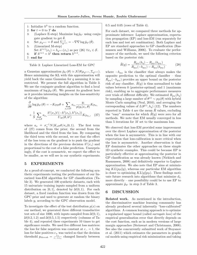
1: Initialize h0 to a random function.2: for t = 0 to T do3: (Laplace E-step) Maximize log pht using conju-

gate gradient to get θ.4: Set µqt+1 = θ and Σ−1

qt+1 = −∇∇ log pht(θ).

5: (Linearized M-step)Set ht+1(xs) = hqt+1(xs) as per (26) ∀xs ∈ S.

6: if ht+1 = ht then return ht+1.7: end for

Table 3: Laplace Linearized Loss-EM for GPC

a Gaussian approximation pht(θ) ' N (θ|µqt+1 ,Σqt+1).Hence minimizing the KL with this approximation willyield back the same Gaussian for q assuming it is un-restricted. We present the full algorithm in Table 3.We use the conjugate gradient algorithm to find a localmaximum of log pht(θ). We present its gradient hereas it provides interesting insights on the loss-sensitivityof the algorithm:

∂

∂θlog pht(θ) = −KDDθ +

∑xi∈D

axi

yip(yi|xi, θ)

KDxi

+1

S

∑xs∈S

axs

ht(xs)` (−ht(xs), ht(xs))UM (θ, ht)

KDxs, (27)

where ax.= σ−1

x N(KxDθ/σx|0, 1). The first termof (27) comes from the prior; the second from thelikelihood and the third from the loss. By comparingthe third term with the second, we see that the effectof the loss term on the gradient is to push the gradientin the directions of the previous decision ht(xs) andproportional to the cost of a false prediction. Unsurpris-ingly, if the cost is symmetric, we expect the effect tobe smaller, as we will see in our synthetic experiments.

5 EXPERIMENTS

As a proof-of-concept, we conducted the following syn-thetic experiments testing the performance of our lin-earized loss-EM algorithm for GP classification (Ta-ble 3). We generated 100 synthetic datasets, each with15 univariate training inputs sampled from a uniformdistribution on [0, 1], denoted by U(0, 1). For eachdataset, a fixed random function was drawn from theGPC prior and used to generate at random the binarylabels yi according to the GPC observation model.

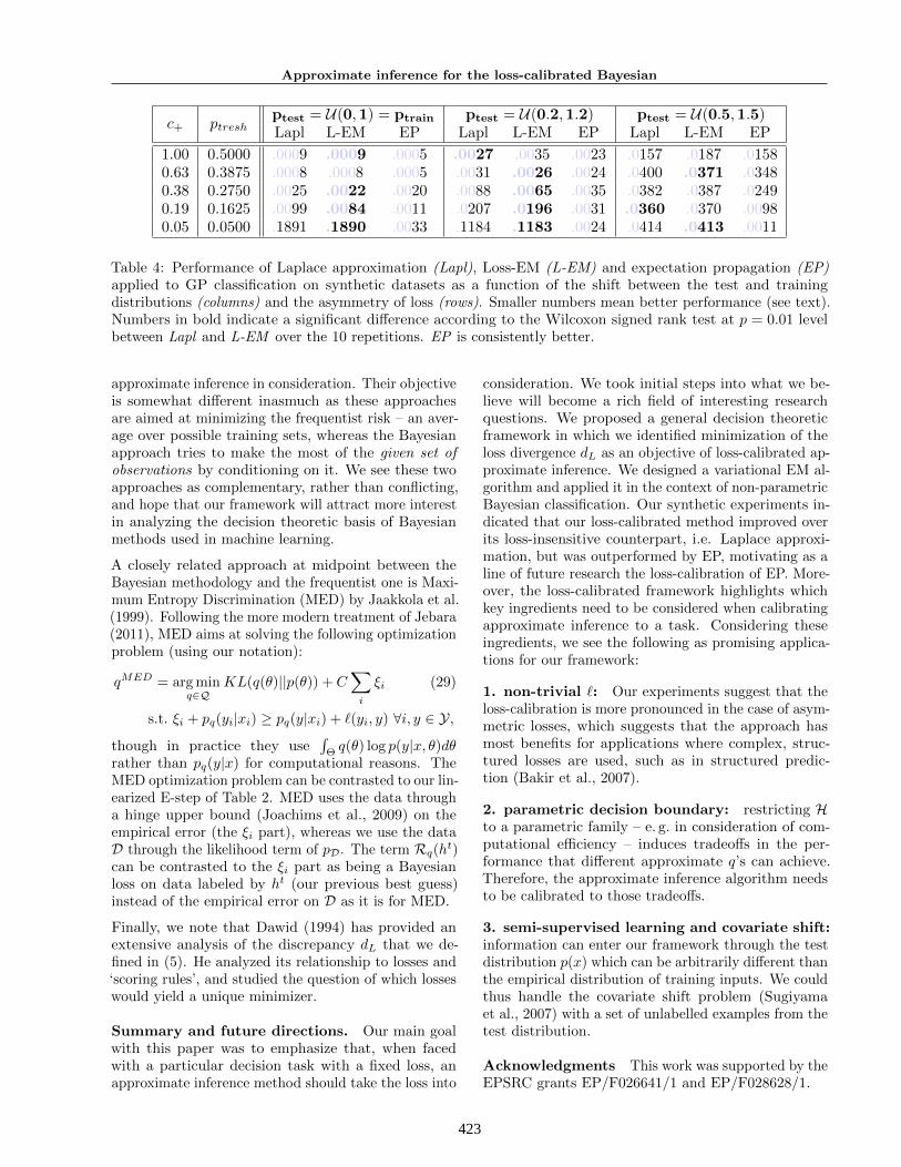
To investigate the effect of the test distribution p(x) onour method, we generated three different transductivetest sets of size 1000, with inputs sampled from U(0, 1),U(0.2, 1.2) and U(0.5, 1.5) respectively (columns of Ta-ble 4), and repeated these experiments 10 times to getsignificance results. We used five different loss matrices:the loss for false negatives was constant at c− = 1, theloss for false positives c+ was varied so that the decisionthreshold pthresh = c+

c−+c+changed linearly between

0.5 and 0.05 (rows of Table 4).

For each dataset, we compared three methods for ap-proximate inference: Laplace approximation, expecta-tion propagation (EP) and loss-EM (run separately foreach loss and test set combination). Both Laplace andEP are standard approaches to GP classification (Ras-mussen and Williams, 2006). To evaluate the perfor-mance of the methods, we used the following criterionbased on the posterior risk:

R(q) =RpD (hq)−RpD (hpD )

RpD (−hpD )−RpD (hpD ). (28)

where −hpD is the classifier that always makes theopposite prediction to the optimal classifier – thusRpD (−hpD ) provides an upper bound on the posterior

risk of any classifier. R(q) is thus normalized to takevalues between 0 (posterior-optimal) and 1 (maximumrisk), enabling us to aggregate performance measuresover trials of different difficulty. We estimated RpD (hq)by sampling a large number of θ(i) ∼ pD(θ) with hybridMonte Carlo sampling (Neal, 2010), and averaging thecorresponding values of L(θ(i), hq) (12). The numbers

reported in Table 4 are the mean R values, excludingthe “easy” scenarios for which R(q) were zero for allmethods. We note that EM usually converged in lessthan 5 iterations for M set to the maximum loss.

We observed that loss-EM provided some improvementover the direct Laplace approximation of the posteriorwhen the loss is asymmetric. This is in line with ourexpectation that loss-calibration is more critical whenthe loss is asymmetric. Another observation is thatEP dominates the other approaches on these simple1D synthetic examples. This could be because EP isparticularly effective at approximating the posterior inGP classification as was already known (Nickisch andRasmussen, 2008) and definitively superior to Laplaceapproximation. We also note that EP aims at minimiz-ing KL(pD‖q), whereas our particular EM algorithmis closer to optimizing KL(q‖pD). These findings moti-vate future research into algorithms that minimize dLmore directly – one possibility could be to use EP toapproximate pht in step 3 of Table 3.

6 DISCUSSION

Related work. As mentioned in the introduction,the discriminative machine learning community hasalready produced several inherently “loss-calibrated”algorithms. A common learning approach is to optimizea regularized upper bound (called surrogate loss) of theempirical generalization error that directly depends onthe cost function, such as in modern versions of largemargin approaches (Steinwart and Christmann, 2008).See also the concurrently submitted work of Stoyanovet al. (2011) which estimates the parameters in graphi-cal models using empirical risk minimization and taking

423

Approximate inference for the loss-calibrated Bayesian

c+ ptreshptest = U(0,1) = ptrain ptest = U(0.2,1.2) ptest = U(0.5,1.5)Lapl L-EM EP Lapl L-EM EP Lapl L-EM EP

1.00 0.5000 .0009 .0009 .0005 .0027 .0035 .0023 .0157 .0187 .01580.63 0.3875 .0008 .0008 .0005 .0031 .0026 .0024 .0400 .0371 .03480.38 0.2750 .0025 .0022 .0020 .0088 .0065 .0035 .0382 .0387 .02490.19 0.1625 .0099 .0084 .0011 .0207 .0196 .0031 .0360 .0370 .00980.05 0.0500 .1891 .1890 .0033 .1184 .1183 .0024 .0414 .0413 .0011

Table 4: Performance of Laplace approximation (Lapl), Loss-EM (L-EM) and expectation propagation (EP)applied to GP classification on synthetic datasets as a function of the shift between the test and trainingdistributions (columns) and the asymmetry of loss (rows). Smaller numbers mean better performance (see text).Numbers in bold indicate a significant difference according to the Wilcoxon signed rank test at p = 0.01 levelbetween Lapl and L-EM over the 10 repetitions. EP is consistently better.

approximate inference in consideration. Their objectiveis somewhat different inasmuch as these approachesare aimed at minimizing the frequentist risk – an aver-age over possible training sets, whereas the Bayesianapproach tries to make the most of the given set ofobservations by conditioning on it. We see these twoapproaches as complementary, rather than conflicting,and hope that our framework will attract more interestin analyzing the decision theoretic basis of Bayesianmethods used in machine learning.

A closely related approach at midpoint between theBayesian methodology and the frequentist one is Maxi-mum Entropy Discrimination (MED) by Jaakkola et al.(1999). Following the more modern treatment of Jebara(2011), MED aims at solving the following optimizationproblem (using our notation):

qMED = arg minq∈Q

KL(q(θ)||p(θ)) + C∑i

ξi (29)

s.t. ξi + pq(yi|xi) ≥ pq(y|xi) + `(yi, y) ∀i, y ∈ Y,

though in practice they use∫

Θq(θ) log p(y|x, θ)dθ

rather than pq(y|x) for computational reasons. TheMED optimization problem can be contrasted to our lin-earized E-step of Table 2. MED uses the data througha hinge upper bound (Joachims et al., 2009) on theempirical error (the ξi part), whereas we use the dataD through the likelihood term of pD. The term Rq(ht)can be contrasted to the ξi part as being a Bayesianloss on data labeled by ht (our previous best guess)instead of the empirical error on D as it is for MED.

Finally, we note that Dawid (1994) has provided anextensive analysis of the discrepancy dL that we de-fined in (5). He analyzed its relationship to losses and‘scoring rules’, and studied the question of which losseswould yield a unique minimizer.

Summary and future directions. Our main goalwith this paper was to emphasize that, when facedwith a particular decision task with a fixed loss, anapproximate inference method should take the loss into

consideration. We took initial steps into what we be-lieve will become a rich field of interesting researchquestions. We proposed a general decision theoreticframework in which we identified minimization of theloss divergence dL as an objective of loss-calibrated ap-proximate inference. We designed a variational EM al-gorithm and applied it in the context of non-parametricBayesian classification. Our synthetic experiments in-dicated that our loss-calibrated method improved overits loss-insensitive counterpart, i.e. Laplace approxi-mation, but was outperformed by EP, motivating as aline of future research the loss-calibration of EP. More-over, the loss-calibrated framework highlights whichkey ingredients need to be considered when calibratingapproximate inference to a task. Considering theseingredients, we see the following as promising applica-tions for our framework:

1. non-trivial `: Our experiments suggest that theloss-calibration is more pronounced in the case of asym-metric losses, which suggests that the approach hasmost benefits for applications where complex, struc-tured losses are used, such as in structured predic-tion (Bakir et al., 2007).

2. parametric decision boundary: restricting Hto a parametric family – e. g. in consideration of com-putational efficiency – induces tradeoffs in the per-formance that different approximate q’s can achieve.Therefore, the approximate inference algorithm needsto be calibrated to those tradeoffs.

3. semi-supervised learning and covariate shift:information can enter our framework through the testdistribution p(x) which can be arbitrarily different thanthe empirical distribution of training inputs. We couldthus handle the covariate shift problem (Sugiyamaet al., 2007) with a set of unlabelled examples from thetest distribution.

Acknowledgments This work was supported by theEPSRC grants EP/F026641/1 and EP/F028628/1.

424

Simon Lacoste-Julien, Ferenc Huszar, Zoubin Ghahramani

References

G. H. Bakir, T. Hofmann, B. Scholkopf, A. J. Smola,B. Taskar, and S. V. N. Vishwanathan. PredictingStructured Data. The MIT Press, 2007.

P. L. Bartlett, M. I. Jordan, and J. D. McAuliffe. Con-vexity, classification, and risk bounds. Journal of theAmerican Statistical Association, 101(473):138–156,2006.

J. O. Berger. Statistical Decision Theory and BayesianAnalysis. Springer, New York, 1985.

L. Csato. Gaussian Processes - Iterative Sparse Ap-proximations. PhD thesis, Aston University, 2002.

A. P. Dawid. Proper measures of discrepancy, uncer-tainty and dependence with applications to predic-tive experimental designs. Technical Report 139,Department of Statistical Science at University Col-lege London, 1994. (revised in 1998).

A. Dempster, N. Laird, and D. Rubin. Maximum like-lihood from incomplete data via the EM algorithm.Journal of the Royal Statistical Society. Series B(Methodological), 39(1):1–38, 1977.

Z. Ghahramani and M. I. Jordan. Factorial hiddenMarkov models. Machine Learning, 29:245–275,1997.

T. Jaakkola, M. Meila, and T. Jebara. Maximum en-tropy discrimination. In Advances in Neural Informa-tion Processing Systems 12. MIT Press, Cambridge,MA, 1999.

T. Jebara. Multitask sparsity via Maximum EntropyDiscrimination. Journal of Machine Learning Re-search, 12:75–110, 2011.

T. Joachims, T. Finley, and C.-N. Yu. Cutting-planetraining of structural SVMs. Machine Learning, 77(1):27–59, 2009.

M. I. Jordan, Z. Ghahramani, T. S. Jaakkola, and L. K.Saul. An introduction to variational methods forgraphical models. In M. I. Jordan, editor, Learningin Graphical Models. MIT Press, Cambridge, 1999.

T. P. Minka. A family of algorithms for approximateBayesian inference. PhD thesis, Massachusetts Insti-tute of Technology, 2001.

R. M. Neal. MCMC using Hamiltonian dynamics. InG. J. S. Brooks, A. Gelman and X.-L. Meng, editors,Handbook of Markov Chain Monte Carlo. Chapman& Hall / CRC Press, 2010.

H. Nickisch and C. E. Rasmussen. Approximations forbinary Gaussian process classification. Journal ofMachine Learning Research, 9:2035–2078, 2008.

J. Quinonero-Candela and C. E. Rasmussen. A uni-fying view of sparse approximate Gaussian processregression. Journal of Machine Learning Research,6:1935–1959, 2005.

C. E. Rasmussen and C. K. I. Williams. GaussianProcesses for Machine Learning. The MIT Press,Cambridge, MA, USA, 2006.

C. P. Robert. The Bayesian Choice. Springer, NewYork, 2001.

M. J. Schervish. Theory of Statistics. Springer, NewYork, 1995.

E. Snelson. Flexible and efficient Gaussian processmodels for machine learning. PhD thesis, GatsbyComputational Neuroscience Unit, University Col-lege London, 2007.

I. Steinwart and A. Christmann. Support Vector Ma-chines. Springer, New York, 2008.

V. Stoyanov, J. Eisner, and A. Ropson. Empirical riskminimization of graphical model parameters givenapproximate inference, decoding, and model struc-ture. In G. Gordon and D. Dunson, editors, Pro-ceedings of the Fourteenth International Conferenceon Artificial Intelligence and Statistics, volume 15,Fort Lauderdale, FL, USA, April 2011. Journal ofMachine Learning Research.

M. Sugiyama, M. Krauledat, and K.-R. Muller. Covari-ate shift adaptation by importance weighted crossvalidation. Journal of Machine Learning Research,8:985–1005, 2007.