UNIVERSITY OF CALIFORNIA, IRVINE Approximate Inference in Graphical Models DISSERTATION submitted in partial satisfaction of the requirements for the degree of DOCTOR OF PHILOSOPHY in Computer Science by Sholeh Forouzan Dissertation Committee: Professor Alexander Ihler, Chair Professor Rina Dechter Professor Charless Fowlkes 2015
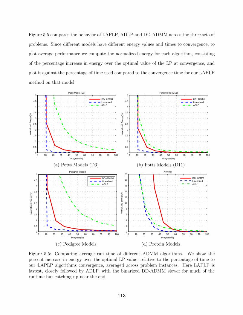
Transcript
UNIVERSITY OF CALIFORNIA,IRVINE
Approximate Inference in Graphical Models
DISSERTATION
submitted in partial satisfaction of the requirementsfor the degree of
DOCTOR OF PHILOSOPHY
in Computer Science
by
Sholeh Forouzan
Dissertation Committee:Professor Alexander Ihler, Chair
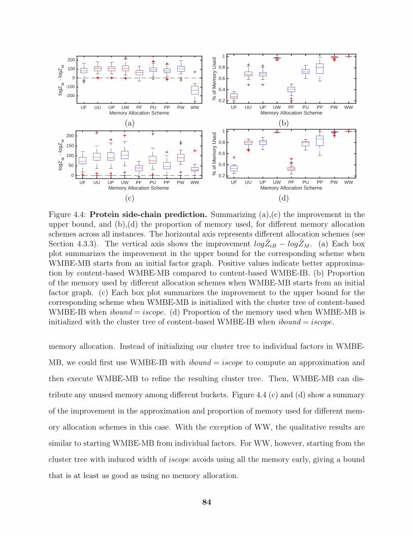
4.1 Memory use, partitioning heuristics, and ibound . . . . . . . . . . . . . . . . 604.2 Incremental WMBE-MB: Updating the memory budget after a merge . . . . 724.3 Memory allocation schemes . . . . . . . . . . . . . . . . . . . . . . . . . . . 754.4 Protein side-chain prediction: Improved approximation and memory use . . . 844.5 Protein side-chain prediction: Different initializations for WMBE-MB . . . . 864.6 Protein side-chain prediction: choice of ibound . . . . . . . . . . . . . . . . . 874.7 Linkage analysis: Improved approximation and memory use . . . . . . . . . 884.8 Linkage analysis: Different initializations for WMBE-MB . . . . . . . . . . . 904.9 WMBE-MB: Memory margin vs potential improvement . . . . . . . . . . . . 904.10 Pedigree instances: Bound quality versus available memory . . . . . . . . . . 914.11 WMBE-MB: Region selection and message passing . . . . . . . . . . . . . . 93
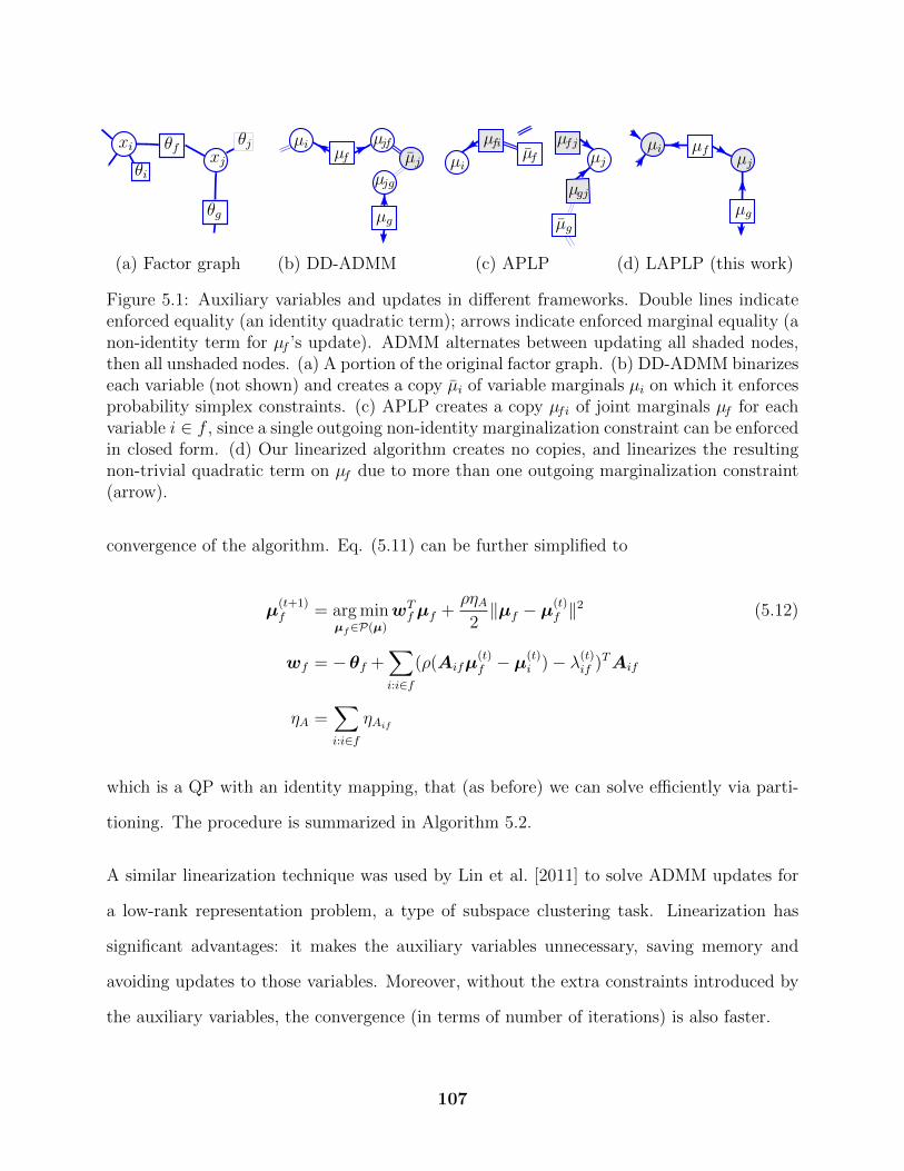
5.1 Auxiliary variables and updates in different frameworks . . . . . . . . . . . . 1075.2 Potts models: Convergence time for LAPLP, DD-ADMM and ADLP . . . . 1105.3 Linkage analysis: Convergence time for LAPLP, DD-ADMM and ADLP . . . 1115.4 Protein side-chain prediction: Convergence time for LAPLP, DD-ADMM and
4.1 Protein side-chain prediction: Improved approximation using WMBE-MB . . 824.2 Protein side-chain prediction: Different initializations for WMBE-MB . . . . 854.3 Linkage analysis: Improved approximation using WMBE-MB . . . . . . . . . 894.4 Linkage analysis: Different initializations for WMBE-MB . . . . . . . . . . . 89
vi
LIST OF ALGORITHMS
Page
2.1 Bucket/Variable Elimination for computing the partition function Z . . . . . 132.2 Bucket/Variable Elimination to compute marginals p(xi) . . . . . . . . . . . 142.3 Mini-Bucket Elimination for computing the partition function Z . . . . . . . 172.4 Weighted Mini-Bucket Elimination for computing the partition function Z . 212.5 Calculating the WMB bound Φ(θ, w) and its derivatives . . . . . . . . . . . 253.1 Incremental region selection for WMBE . . . . . . . . . . . . . . . . . . . . . 403.2 AddRegions: find regions to add for merge . . . . . . . . . . . . . . . . . . . 443.3 MergeRegions: merge and parameterize newly added regions to improve bound 464.1 Memory-aware region selection using ibound . . . . . . . . . . . . . . . . . . 644.2 Memory-aware Incremental region selection for WMBE using ibound . . . . . 654.3 Memory-aware Incremental region selection for WMBE using memory budget 694.4 Memory-aware region selection using memory budget . . . . . . . . . . . . . 704.5 Updating memory budget after adding new regions . . . . . . . . . . . . . . 704.6 Checking memory required for adding a new region . . . . . . . . . . . . . . 794.7 Checking memory required for adding a new region under memory budget . 805.1 Efficient projection on to the l ball . . . . . . . . . . . . . . . . . . . . . . 1045.2 Linearized APLP . . . . . . . . . . . . . . . . . . . . . . . . . . . . . . . . . 106
vii
ACKNOWLEDGMENTS
How does a person say thank you, when there are so many people to thank. First andforemost I would like to thank my advisor Prof. Alexander Ihler without whom this journeywas not possible. Not only he was a brilliant research advisor to me, but he was also agreat mentor and an incredible source of support when I needed it the most. His timelyencouragements helped me grow beyond what I thought was possible. I’ve learned a lotfrom him, academically and otherwise and will forever be in depth to him.
I would also like to thank my committee members Prof. Rina Dechter and Prof. CharlessFowlkes, for their time and feedback. Rina’s research and teachings were the building blocksof this thesis. She always made sure that I could reach out to her for advice and helpedme with her constructive feedback. Charless inspired my interest in computer vision andconstantly amazed me by his intuition and his ability to explain any complicated idea verysimply. I was fortunate to do research with him and learned a lot from him.
I am also indebted to Dr. Babak Shahbaba and Dr. Payam Heydari for being there for meduring this journey. They encouraged me to follow my passion every step of the way. Theirinsights and encouragement were one of the things that supported me when I needed it themost.
Of course, my experience at UCI was largely shaped by my peers. I’d like to thank thestudents from Machine Learning and Vision Labs and most importantly members of IGBwho brought me up to speed when I first came to UCI.
Last, and most importantly, I want to thank my wonderful family. They all believed inme through out this journey which gave me the confidence I needed to make it to the end.Finally to my ever-supportive husband who stood by my side every step of the way, throughthe good and the bad. His unconditional support was the single most important reason Imade it through the end and I am forever indebted to him for that.
I am grateful for the assistance I have received for my graduate studies from NSF grants IIS-1065618 and IIS-1254071, and by the United States Air Force under Contract No. FA8750-14-C-0011 under the DARPA PPAML program.
viii
CURRICULUM VITAE
Sholeh Forouzan
EDUCATION
Ph.D in Computer Science 2015University of California, Irvine Irvine, CA
M.S in Computer Science 2011University of California, Irvine Irvine, CA
M.S in AI and Robotics 2008University of Tehran Tehran, Iran
B.S in Computer Engineering 2006Shahid Beheshti University Tehran, Iran
ix
ABSTRACT OF THE DISSERTATION
Approximate Inference in Graphical Models
By
Sholeh Forouzan
Doctor of Philosophy in Computer Science
University of California, Irvine, 2015
Professor Alexander Ihler, Chair
Graphical models have become a central paradigm for knowledge representation and rea-
soning over models with large numbers of variables. Any useful application of these models
involves inference, or reasoning about the state of the underlying variables and quantify-
ing the models’ uncertainty about any assignment to them. Unfortunately, exact inference
in graphical models is fundamentally intractable, which has led to significant interest in
approximate inference algorithms.
In this thesis we address several aspects of approximate inference that affect its quality. First,
combining the ideas from variational inference and message passing on graphical models, we
study how the regions over which the approximation is formed can be selected more effectively
using a content-based scoring function that computes a local measure of the improvement
to the upper bound to log partition function. We then extend this framework to use the
available memory more efficiently, and show that this leads to better approximations. We
propose different memory allocation strategies and empirically show how they can improve
the quality of the approximation to the upper bound. Finally, we address the optimization
algorithms used in approximate inference tasks. Focusing on maximum a posteriori (MAP)
inference and linear programming (LP), we show how the Alternating Direction Method of
Multipliers (ADMM) technique can provide an elegant algorithm for finding the saddle point
x
of the augmented Lagrangian of the approximation, and present an ADMM-based algorithm
to solve the primal form of the MAP-LP whose closed form updates are based on a linear
approximation technique.
xi
Chapter 1
Introduction
Graphical models are a powerful paradigm for knowledge representation and reasoning. Well
known examples of graphical models include Bayesian networks, Markov random fields, con-
straint networks and influence diagrams. An early application of graphical models in com-
puter science is medical diagnostics, in which medical specialists are interested in diagnosing
the disease a patient might have by reasoning about the possible causes of a set of observed
symptoms, or evaluate which future tests might best resolve the patient’s underlying dis-
eases. Another popular example application of graphical models is in computer vision, such
as image segmentation and classification, where each image might consist of thousands of
pixels and the goal is to figure out what type of object each pixel corresponds to.
To model such problems using graphical models, we represent them by a set of random
variables, each of which represent some facet of the problem. Our goal is then to capture
the uncertainty about the possible states of the world in terms of the joint probability
distribution over all assignments to the set of random variables.
One of the main characteristics of such models is that there is going to be some significant
uncertainty about the correct answer. Probability theory is used to deal with such uncer-
tainty in a principled way by providing us with probability distributions as a declarative
representation with clear semantics, accompanied by a toolbox of powerful reasoning pat-
1
terns like conditioning, as well as a range of powerful learning methodologies to learn the
models from data.
While probability theory deals with modeling the uncertainty in such problems, in most
cases we are still faced with another complexity: the very large number of variables to
reason about. Even for the simplest case where each random variable is binary, for a system
with n variables the joint distribution will have 2n states, which requires us to deal with
representations that are intrinsically exponentially large. For these computational reasons,
we exploit ideas from computer science, specifically graphs, to encode structure within this
distribution and exploit the structure to represent and manipulate the distribution efficiently.
The resulting graphical representation gives us an intuitive and compact data structure
to encode high dimensional probability distributions, as well as a suite of methods that
exploit the graphical structure for efficient reasoning. At the same time, the graph structure
allows the parameters of the probability distribution to be encoded compactly, representing
high dimensional probability distributions using a small number of parameters and allowing
efficient learning of the parameters from data.
From this point of view, graphical models combine ideas from probability theory and ideas
from computer science to provides powerful tools for describing the structure of a probability
distribution and to organize the computations involved in reasoning about it. As a result,
this framework has been used in a broad range of applications in areas including coding and
information theory, signal and image processing, data mining, computational biology and
computer vision.
2
1.1 Examples of graphical models
Protein side chain prediction. Predicting side-chain conformation given the backbone
structure is a central problem in protein-folding and molecular design. Proteins are chains of
simpler molecules called amino acids. All amino acids have a common structure - a central
carbon atom (COl) to which a hydrogen atom, an amino group (NH2) and a carboxyl group
(COOH) are bonded. In addition, each amino acid has a chemical group called the side-
chain, bound to COl. This group distinguishes one amino acid from another and gives
its distinctive properties. Amino acids are joined end to end during protein synthesis by
the formation of peptide bonds. An amino acid unit in a protein is called a residue. The
formation of a succession of peptide bonds generate the backbone (consisting of COl and its
adjacent atoms, N and CO, of each reside), upon which the side-chains are hung [Yanover
and Weiss, 2003].
The goal of molecular design is then to predict the configuration of all the side-chains relative
to the backbone. The standard approach to this problem is to define an energy function and
use the configuration that achieves the global minimum of the energy as the prediction.
To model this problem, a random variable is defined for each residue and the state of it
represents the configuration of the side-chain of that residue. The factors in graphical model
then capture the constraints and the energy of the interactions with the goal of finding
a configuration that achieves the global minimum of the energy defined over the factors
[Yanover and Weiss, 2003].
Genetic linkage analysis. In human genetic linkage analysis, the haplotype is the sequence
of alleles at different loci inherited by an individual from one parent, and the two haplotypes
(maternal and paternal) of an individual constitute that individual’s genotype. However,
this inheritance process is not easily observed. Measurement of the genotype of an indi-
vidual typically results in a list of unordered pairs of alleles, one pair for each locus. This
3
information must be combined with pedigree data (a family tree of parent/offspring relation-
ships) in order to estimate the underlying inheritance process [Fishelson and Geiger, 2002].
A graphical model representation of given pedigree of individuals with marker information
(alleles at different loci) takes the form of a Bayesian network with variables representing the
genotypes, phenotypes, and selection of maternal or paternal allele for each individual and
locus. Finding the haplotype of individuals translates to an optimization task of finding the
most probable explanation (mpe) of the Bayesian network. Another central task is linkage
analysis, which seeks to find the loci on the chromosome that are associated with a given
disease. This question can be answered by finding the probability of evidence over a very
similar Bayesian network [Fishelson and Geiger, 2002].
1.2 Inference
Inference in graphical models refers to reasoning about the state of the underlying variables
and quantifying the model’s uncertainty about any assignment to the random variables.
For example, given the graphical model, we might be interested in finding the most likely
configuration of variables and its value. This is an inference task that comes up in protein
side-chain prediction, where the goal is then to find a configuration that achieves the maxi-
mum value of the objective function and recover optimal amino acid side-chain orientations
in a fixed protein backbone structure.
Another equally important inference task is computing summations (marginalizing) over
variables. Such inference task comes up when computing the marginal probability of a
variable being in any of its states and computing the partition function. Both of these tasks
are essential parts of training conditional random fields for image classification where we
need to compute the partition function and the marginal distributions in order to evaluate
the likelihood and its derivative. More importantly, because both of these quantities should
4
be computed for each training instance every time the likelihood is computed, we need to
have efficient methods for it.
Unfortunately, like many interesting problems, inference in graphical models is NP-hard
[Koller and Friedman, 2009a] as there are exponentially large number of possible assignments
to the variables in the models. Despite such complexity, inference can be performed exactly
in polynomial time for some graphical models that have simple structure like trees. The
most popular exact algorithm, the junction tree algorithm, groups variables into clusters
until the graph becomes a tree. Once an equivalent tree has been constructed, its marginals
can be computed using exact inference algorithms that are specific to trees.
However, many interesting problems that arise ubiquitously in scientific computation are
not amenable to such simple algorithm. For many real-world problems the junction tree
algorithm is forced to make clusters which are very large and the inference procedure still
requires exponential time in the worst case. Such complexity have inspired significant interest
in approximate inference algorithms and had led to significant advances in approximation
methods in the past decade.
1.3 Approximate Inference
The complexity of exact inference have led to significant interest in approximate inference
algorithms. Monte Carlo algorithms and variational methods are the two main classes that
received the most attention. Monte Carlo algorithms are stochastic algorithms that attempt
to produce samples from the distribution of interest. Variational algorithms on the other
hand convert the inference problem into an optimization problem, trying to find a simple
approximation that most closely matches the intractable marginals of interest. Generally,
Monte Carlo algorithms are unbiased and given enough time, are guaranteed to sample from
5
the distribution of interest. However, in practice, it is generally impossible to know when that
point of time has been reached. Variational algorithms, on the other hand, tend to be much
faster, but they are inherently biased. In other words, not matter how much computation
time they are given, they can not lesson the error that is inherent to the approximation.
1.4 Summary of Contributions
Our ultimate goal is to advance the computational capabilities of reasoning algorithms for
intelligent systems using the graphical models framework. We consider graphical models
that involve discrete random variables and develop methods that allow us to improve on the
existing approximate inference algorithms in several dimensions. We focus our attention to
several areas that affect the quality of approximate inference:
• finding better approximations to the exponentially hard exact inference problem
• finding more efficient ways to use the available memory to improve the approximation
• finding better optimization algorithms to solve the approximate inference task faster
and more accurately
As stated earlier an inherent source of error in variational methods is the approximation
itself and thus finding better approximations is the key to reducing the error in the inference
task. We show how such an approximation can be built incrementally in the context of
weighted mini-bucket elimination for computing the partition function. We also study how
approximate inference algorithms based on mini-bucket elimination use the available mem-
ory and develop algorithms that allows efficient use of the amount of memory available to
construct better approximations and hence better approximate inference. Finally we focus
our attention on the algorithms used to solve the optimization task for approximate inference
6
and develop an algorithm that uses Alternative direction method of multipliers (ADMM), a
state of the art optimization algorithm, to find better solutions to the approximate inference
problem for computing the maximizing assignment to variables.
To do so, this thesis first presents some background on problems and methods for graphical
models in Chapter 2, then describes our contributions in three parts:
Chapter 3:
• We describe how to use the message passing framework of Weighted Mini-bucket Elim-
ination(WMBE) to select better regions to define the approximation and improve the
bound
• We introduce a new merging heuristic for (weighted) mini-bucket elimination that uses
message passing optimization of the bound, and variational interpretations, in order
to construct a better heuristic for selecting moderate to large regions in an intelligent,
energy-based way
• We propose an efficient structure update procedure that incrementally updates the join
graph of mini-bucket elimination after new regions are added in order to avoid starting
from scratch after each merge.
Chapter 4:
• We describe how controlling the complexity of inference using ibound can result in
inefficient use of resources and propose memory-aware alternatives
• We propose several memory allocation techniques to bypass the choice of a single
control parameter for content-based MBE approximation that allows a more flexible
control of memory during inference
7
• We expand the incremental region selection algorithm for weighted mini-bucket elimi-
nation to use a more fine tuned memory budget rather than a fixed ibound
• We perform an empirical evaluation of different allocation schemes, characterizing their
behavior in practice
• We propose practical guidelines for choosing the memory allocation scheme for different
classes of problems
Chapter 5:
• We present an algorithm based on the Alternating Direction Method of Multipliers
(ADMM) for approximate MAP inference using its linear programming relaxation
• We characterize different formulations of such problem using a graphical approach and
discuss the challenges
• We propose a linear approximation to ADMM that allows solving the optimization
efficiently
8
Chapter 2
Background
Graphical models capture the dependencies among large numbers of random variables by
explicitly representing the independence structure of the joint probability distribution. It
is useful to represent probability distributions using the notion of factor graphs. Such a
representation allows the inference algorithms to be applied equally well to Bayesian networks
and Markov random fields, as both of those can be easily converted to factor graphs.
For example, the factor graph in Figure 2.1 represents the joint distribution over random
variables X1, . . . , X5 as a collection of factors fij(Xi, Xj) over pairs of variables. Each random
variable Xi can take one of several possible values xi ∈ Xi, where Xi is called the domain
and |Xi| is called the cardinality of the variable. A factor f(X1, . . . , XN) is then a function
(or table) that takes a set of random variables {X1, . . . , XN} as input, and returns a value
for every assignment, (x1, . . . , xN), to those random variables in the cross product space
(a) (b)
Figure 2.1: (a) Factor graph (b) Factor
9
X = X1×· · ·×XN . In the sequel, we use var(f) to refer to the set of input random variables,
{X1, . . . , XN}, for factor f(X1, . . . , XN). By this definition, a factor can be normalized,
i.e.∑
xαf(xα) = 1 and f(xα) ≥ 0 for all assignments xα, or may be un-normalized so
that it does not necessarily correspond to a probability distribution. These factors are
the fundamental building blocks in defining distributions in a high dimensional space. A
probability distribution over a large set of variables is then formed by multiplying factors:
p(x1, . . . , xN) = p(x) =1
Z
∏α∈I
fα(xα) where Z =∑
x
∏α
fα(xα)
Here xα indicates the subset of variables that appear as arguments to factor fα, and Z is
a constant which serves to normalize the distribution (called the partition function). We
assume f(xα) ≥ 0. As shown in Figure 2.1, we can then associate p(x) with a graph
G = (V,E), where each variable Xi is associated with a node of the graph G. The node
corresponding to Xi is connected to Xj if both variables are arguments of some factor fα(xα).
The set I is then a set of fully connected cliques in G.
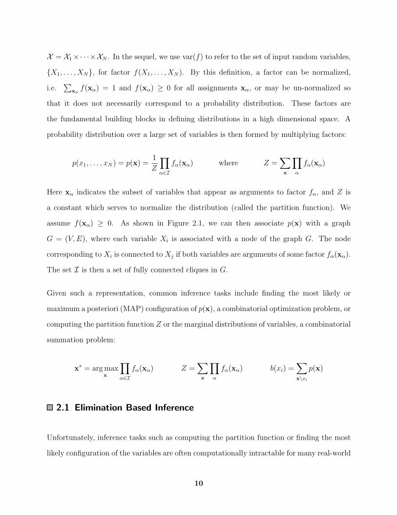
Given such a representation, common inference tasks include finding the most likely or
maximum a posteriori (MAP) configuration of p(x), a combinatorial optimization problem, or
computing the partition function Z or the marginal distributions of variables, a combinatorial
summation problem:
x∗ = arg maxx
∏α∈I
fα(xα) Z =∑
x
∏α
fα(xα) b(xi) =∑x\xi
p(x)
2.1 Elimination Based Inference
Unfortunately, inference tasks such as computing the partition function or finding the most
likely configuration of the variables are often computationally intractable for many real-world
10
problems. Elimination based methods such for exact inference, such as variable or ‘bucket’
elimination [Dechter, 1999] directly eliminate (by summing or maximizing) the variables,
one at a time, along a predefined elimination ordering. The complexity of such an elimi-
nation procedure is exponential in the tree-width of the model, leading to a spectrum of
approximations and bounds subject to computational limits. We first introduce the bucket
elimination method [Dechter, 1999] in Section 2.1.1 and then the mini-bucket elimination
method [Dechter and Rish, 2003] for approximate inference. We mainly focus our discus-
sion on marginal inference, but the same methods can be applied to maximization tasks by
replacing the sum operator with max.
2.1.1 Bucket Elimination
Bucket elimination (BE) [Dechter, 1999] is an exact algorithm that directly eliminates vari-
ables in sequence. Given an elimination order, BE collects all factors that include variable Xi
as their earliest-eliminated argument in a bucket Bi, then takes their product and eliminates
Xi to produce a new factor over later variables, which is placed in the bucket of its “parent”
πi, associated with the earliest uneliminated variable:
λi→πi(xi→πi) =∑xi
∏fα∈Bi
fα(xα)∏
λj→i∈Bi
λj→i(xj→i)
where xi→πi is the set of variables that remain in the scope of the intermediate functions
λi→πi after Xi is eliminated. This calculation can be conveniently organized as a “Bucket
Elimination” procedure shown in Algorithm 2.1.
As an example, for the toy model of Figure 2.1, the BE algorithm takes the following steps:
Given the elimination order o = [1, 2, 3, 4, 5], the bucket elimination algorithm starts by
eliminating variable X1 by grouping all factors containing X1 in their scope, in bucket B1
11
(a) (b)
Figure 2.2: (a) Bucket Elimination (b) The Cluster Tree for Bucket Elimination
and eliminating X1 by
λ1→π1(x2, x3, x4) =∑x1
f12f13f14,
where we use fij as shorthand for fij(xi, xj). The elimination results in the intermediate
function, λ1→π1 . This intermediate function is then passed to bucket B2 (associated with
variable X2), which is the first variable that will be eliminated from this function based on
the elimination order o. Figure 2.2(a) shows how the original factors are grouped together in
the buckets and how the messages generated by the algorithm are assigned to each bucket.
Execution of Bucket elimination algorithm induces a tree structure, CT = (V,E), known as
a cluster tree. The cluster tree then associates a node i ∈ V to each bucket Bi. An edge
(i, j) ∈ E connects the two nodes i and j if the intermediate function λi→πi produced by
processing bucket Bi is passed to bucket Bj.
From the cluster tree prespective, the functions λi→πi constructed during the elimination
process can be interpreted as messages that are passed downward in a cluster tree represen-
tation of the model [Ihler et al., 2012]; see Figure 2.2(b). We will refer to bucket B2 as being
12
Algorithm 2.1 Bucket/Variable Elimination for computing the partition function Z
Input: Set of factors of a graphical model F = {fα(xα)}, an elimination order o =[x1, . . . , xN ]Output: The partition function Zfor i← 1 to N do
Find the set (bucket) Bi of factors fα and intermediate messages λj→i over variable xi.
Eliminate variable xi:
λi→πi(xi→πi) =∑xi
∏fα∈Bi
fα(xα)∏
λj→i∈Bi
λj→i(xj→i)
Update the factor list F← {F−Bi} ∪ {λi→πi(xi→πi)}:
end forReturn: partition function Z =
∏λi→∅∈F
λi→∅
the parent of bucket B1 and bucket B1 as being a child of bucket B2. Note that a bucket
may have multiple children, but can only have one parent.
Note that while computing the partition function of the probability distribution over the
variables {X1 . . . X5} using a brute-force procedure requires a sum over a 5 dimensional
tensor with computational complexity O(k5), where k is the number of possible states for
Xi, the bucket elimination complexity is only O(k4).
In general, the space and time complexity of BE are exponential in the induced width of
the graph along the elimination order, which is the maximum number of variables that
appear together in a bucket and need to be reasoned about jointly. While good elimination
orders can be identified using various heuristics [see e.g., Kask et al., 2011], this exponential
dependence often makes direct application of BE intractable for many problems of interest.
Computing Marginal Probabilities
13
Algorithm 2.2 Bucket/Variable Elimination to compute marginals p(xi) [Dechter, 1999]
Input: Set of factors of a graphical model F = {fα(xα)}, an elimination order o =[x1, . . . , xN ]Output: The partition function Z and the marginal distributions {p(xBi)}Forward Pass: Use Algorithm 2.1 to calculate Z and all the messages λi→πi for all bucketsBi
Backward Pass:
Initialize p(xBi) =∏fα∈Bi
fα(xα)∏
λj→i∈Bi
λj→i(xj→i)
for j ← N − 1 to 1 do
Compute a message from Bj to Bi; where Bj is the bucket that receives the messageλi→πi in the forward elimination
λj→i(xj→i) =∑
xBj \xBi
p(xBj)
λi→πi(xi→πi)
Compute the marginal over variables in Bi:
p(xBi) = λj→i(xj→i)p(xBi)
end forReturn: partition function Z and the marginals {p(xBi)}Remark: Marginals over single variables can be computed by further marginalizing overthe variables in the bucket. e.g. p(xi) =
∑πip(xBi)
In many cases we are interested in calculating the marginal probabilities, p(xi). To do so
we can simply fix the value xi and run the BE Algorithm 2.1 for all possible values of
xi. While simple, such approach is very inefficient as we often need to compute p(xi) for all
variables and all their possible values which repeat many of the same calculations. By sharing
the repeated calculations, one can derive a more efficient algorithm. Dechter [1999] shows
how an additional backward elimination can be used to compute the marginal probabilities
recursively; this procedure is shown as Algorithm 2.2.
14
2.1.2 Mini-bucket Elimination.
To avoid the complexity of bucket elimination, Dechter and Rish [2003] proposed an approx-
imation in which the factors in bucket Bi are grouped into partitions Qi = {q1i , ..., q
pi }, where
each partition qji ∈ Qi, also called a mini-bucket, includes no more than ibound + 1 variables.
The user-selected bounding parameter ibound then serves as a way to control the complex-
ity of elimination, as the elimination operator is applied to each mini-bucket separately.
The ibound parameter then provides a flexible method to trade off between complexity and
accuracy.
For the running example of Figure 2.1, the elimination process for X1,∑
x1f12f13f14, can
be approximated by the following upper and lower bounds to the exact elimination [Dechter
and Rish, 2003]:
∑x1
f12f13 minx1
f14 ≤∑x1
f12f13f14 ≤∑x1
f12f13 maxx1
f14,
which holds for all values of (x2, x3, x4). Mini-bucket approximation eliminatesX1 from f12f13
and f14 separately, instead of eliminating X1 from their product f12f13f14; this reduces the
computational complexity from O(k4) to O(k3), as the separate eliminations operate over
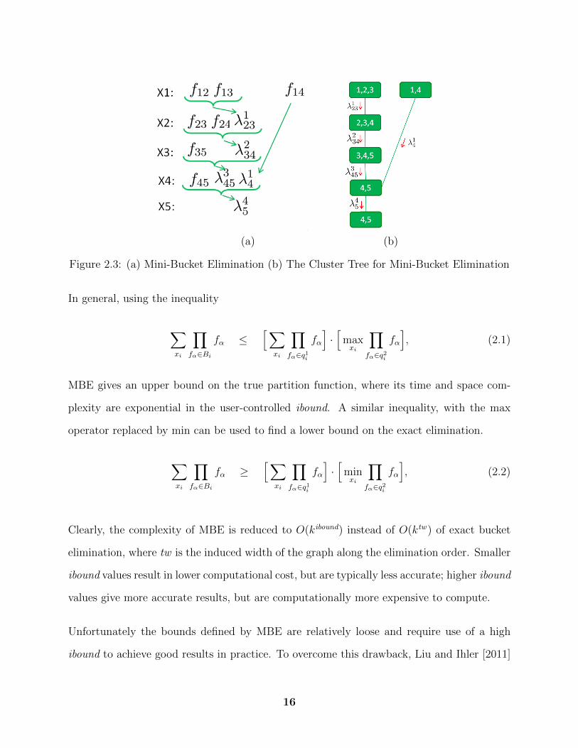
smaller functions. Figure 2.3 (a) shows mini-bucket elimination with ibound = 2 and Figure
2.3 (b) shows the cluster tree generated along the elimination procedure.
More generally, this approximation can be applied within each elimination step of Bucket
Elimination (Algorithm 2.1), which results in a general mini-bucket elimination (MBE) al-
gorithm given in Algorithm 2.3 [Dechter and Rish, 2003]. At each elimination step, MBE
first splits the functions in the bucket Bi into smaller mini-buckets (partitions) and then
eliminates Xi from each mini-bucket separately. The results are then passed to buckets later
in the elimination order.
15
(a) (b)
Figure 2.3: (a) Mini-Bucket Elimination (b) The Cluster Tree for Mini-Bucket Elimination
In general, using the inequality
∑xi
∏fα∈Bi
fα ≤[∑
xi
∏fα∈q1
i
fα
]·[
maxxi
∏fα∈q2
i
fα
], (2.1)
MBE gives an upper bound on the true partition function, where its time and space com-
plexity are exponential in the user-controlled ibound. A similar inequality, with the max
operator replaced by min can be used to find a lower bound on the exact elimination.
∑xi
∏fα∈Bi
fα ≥[∑
xi
∏fα∈q1
i
fα
]·[
minxi
∏fα∈q2
i
fα
], (2.2)
Clearly, the complexity of MBE is reduced to O(kibound) instead of O(ktw) of exact bucket
elimination, where tw is the induced width of the graph along the elimination order. Smaller
ibound values result in lower computational cost, but are typically less accurate; higher ibound
values give more accurate results, but are computationally more expensive to compute.
Unfortunately the bounds defined by MBE are relatively loose and require use of a high
ibound to achieve good results in practice. To overcome this drawback, Liu and Ihler [2011]
16
Algorithm 2.3 Mini-Bucket Elimination for computing the partition function Z[Dechter and Rish, 2003]
Input: Set of factors of a graphical model F = {fα(xα)}, an elimination order o =[x1, . . . , xN ], and an iboundOutput: An upper (lower) bound on partition function Zfor i← 1 to N do
Find the set (bucket) Bi of factors fα and intermediate messages λj→i over variable xi.
Partition Bi into p subgroups q1i , . . . , q
pi such that ∪pj=1q
ji = Bi and
| ∪f∈qji var(f)| ≤ ibound + 1 for all j = 1, . . . , p
Eliminate variable xi:for m = 1 . . . p do
λi→πi(xi→πi) =
∑xi
(∏fα∈qmi
fα(xα)∏
λj→i∈qmi
λj→i(xj→i)), if m = 1
maxxi
(∏fα∈qmi
fα(xα)∏
λj→i∈qmi
λj→i(xj→i)), if m 6= 1
end for
Update the factor list F← {F−Bi} ∪ {λi→πi(xi→πi)}:
end forReturn: the bound on partition function Z =
∏λi→∅∈F
λi→∅
Remark: A lower bound can be obtained by replacing the max in elimination step withmin
introduced weighted mini-bucket elimination which uses a more general bound based on
Hollder’s inequality that can give tighter bounds for small ibound values. The details of
weighted MBE are explained in section 2.1.3.
It is important to highlight the relationship between miini-bucket elimination and message
passing, as mini-bucket elimination can be interpreted in the context of a cluster tree and
message passing on it. The corresponding cluster tree for a particular partitioning then
17
contains a cluster for each mini-bucket, with its scope being the union of the scope of all
the factors in that mini-bucket, and MBE bound corresponds to a problem relaxation in
which a copy of shared variables between the mini-buckets is made for each, and the result
of eliminations λi→πis correspond to the messages in a cluster tree defined on the augmented
model over the variable copies; see Figure 2.3(b). This cluster tree is guaranteed to have
induced-width ibound or less. The problems are equivalent if all copies of Xi are constrained
to be equal; otherwise, the additional degrees of freedom lead to a relaxed problem and thus
can generate an upper bound. This connection allows us to apply any of the message passing
paradigms to our inference problem and inspires combining message passing techniques with
MBE based approximate inference techniques and balance the positive properties of both.
Another factor that affects the mini-bucket bound significantly is the choice of partitions Qi.
In Chapter 3, we explain the existing heuristics that have been used to guide the choice of
partitions, and introduce a new general partitioning heuristic within weighted mini-bucket
that results in better approximation quality.
2.1.3 Weighted Mini-bucket
A recent improvement to mini-bucket generalizes the MBE bound with a “weighted” elimina-
tion [Liu and Ihler, 2011]. Compared to standard MBE, which approximates the intractable
summation operators with upper/lower bounds based on max/min operators, weighted mini-
bucket builds an approximation based on the more general powered sum with a “weighted”
elimination step. An upper or lower bound can then be computed depending on the signs of
the weights.
Weighted mini-bucket applies Holder’s and reverse Holder inequalities, which provide gen-
eral tools for constructing bounds or approximations to the sum of products, to form the
foundation for of a mini-bucket approximation [Liu and Ihler, 2011]. For a set of positive
18
functions fα(xα), α = 1, . . . , n defined over discrete variables x, and a set of non-zero weights
w = [w1, . . . , wn], Holder’s inequality results in an upper bound
∑x
∏α
fα ≤∏r
[∑xi
f1wrα
]wrfor w ∈ W+ (2.3)
and reverse Holder’s inequality results in a lower bound
∑x
∏α
fα ≥∏r
[∑xi
f1wrα
]wrfor w ∈ W− (2.4)
where
W+ = {w :∑r
wr = 1 and wr > 0,∀r = 1, . . . , n}
W− = ∪nk=1W−k where W−k = {w :∑r
wr = 1 and wk > 0, wr < 0,∀r 6= k}
so that W+ corresponds to a probability simplex on the weights wr, and W− corresponds
to a normalized weights with exactly one positive element. Given equations (2.3) and (2.4),
the sum of products of functions can be approximated using products of powered sums over
individual functions and can be used to provide upper and lower bounds for the partition
function in a manner similar to mini-bucket elimination.
For the running example of Figure 2.1, weighted mini-bucket approximation results in the
following elimination, where w1 and w2 are weights satisfying w1 +w2 = 1 and the direction
of inequality depends on the signs of the weights [w1, w2].
∑x1
f12f13f14≥≤ [
∑x1
(f12f13)1w1 ]w1 [
∑x1
f1w2
14 ]w2
It is interesting to note that the powered sumw∑x
f(x) =(∑
x
f(x)1w
)wapproaches max
xf(x)
19
when w → 0+ and minxf(x) as w → 0. Consider the upper bound of equation (2.3) for a
partition q1i , q
2i , which takes the form
∑xi
∏fα∈Bi
fα ≤[∑
xi
∏fα∈q1
i
f1w1α
]w1
·[∑
xi
∏fα∈q2
i
f1w2α
]w2
,
where wi > 0 and w1 + w2 = 1. It is easy to see that this bound generalizes the mini-
bucket upper bound where w1 = 1 and w2 → 0+. The same argument holds for the lower
bound (2.4), as it generalizes the mini-bucket lower bound where w1 = 1 and w2 → 0−.
Based on these Holder inequality bounds, Liu and Ihler [2011] then generalized mini-bucket
elimination to weighted mini-bucket elimination (WMB), presented in Algorithm 2.4, by
replacing the mini-bucket bound with Holder’s inequality. The general procedure is the same,
except that the sum/max operators are replaced with weighted sums where the weights are
normalized to sum to one for each variable.
Liu and Ihler [2011] also show that the resulting bound is equivalent to a class of bounds based
on tree reweighted (TRW) belief propagation [Wainwright et al., 2005], or more generally
conditional entropy decompositions (CED) [Globerson and Jaakkola, 2007a], on a join-graph
defined by the mini-bucket procedure. This connection is used to derive fixed point repa-
rameterization updates, which change the relative values of the factors fα while keeping
their product constant in order to tighten the bound. Section 2.2 gives some background on
variational methods for inference and further explains this connection.
Variable Splitting Perspective
It is useful to consider the effect of partitioning of functions into different mini-buckets
and eliminating in each mini-bucket separately. This procedure effectively splits a variable
into one or more replicates, one for each mini-bucket. From this perspective, mini-bucket
20
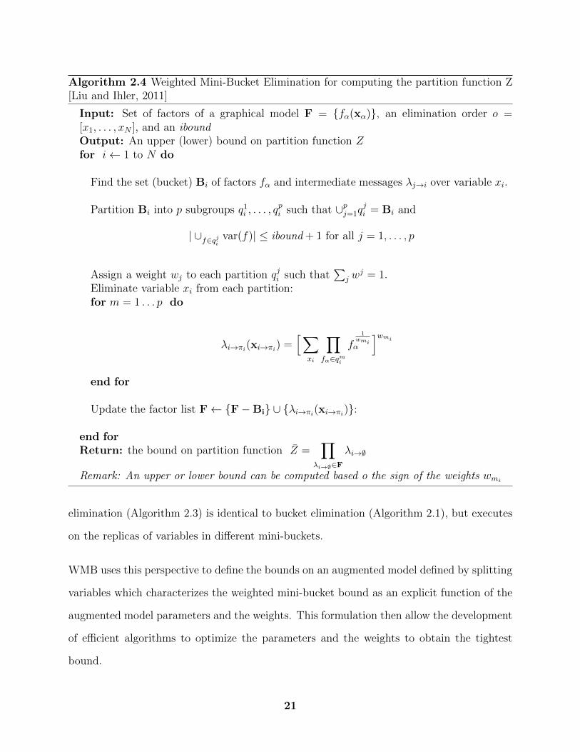
Algorithm 2.4 Weighted Mini-Bucket Elimination for computing the partition function Z[Liu and Ihler, 2011]
Input: Set of factors of a graphical model F = {fα(xα)}, an elimination order o =[x1, . . . , xN ], and an iboundOutput: An upper (lower) bound on partition function Zfor i← 1 to N do
Find the set (bucket) Bi of factors fα and intermediate messages λj→i over variable xi.
Partition Bi into p subgroups q1i , . . . , q
pi such that ∪pj=1q
ji = Bi and
| ∪f∈qji var(f)| ≤ ibound + 1 for all j = 1, . . . , p
Assign a weight wj to each partition qji such that∑
j wj = 1.
Eliminate variable xi from each partition:for m = 1 . . . p do
λi→πi(xi→πi) =[∑
xi
∏fα∈qmi
f1
wmiα
]wmiend for
Update the factor list F← {F−Bi} ∪ {λi→πi(xi→πi)}:
end forReturn: the bound on partition function Z =
∏λi→∅∈F
λi→∅
Remark: An upper or lower bound can be computed based o the sign of the weights wmi
elimination (Algorithm 2.3) is identical to bucket elimination (Algorithm 2.1), but executes
on the replicas of variables in different mini-buckets.
WMB uses this perspective to define the bounds on an augmented model defined by splitting
variables which characterizes the weighted mini-bucket bound as an explicit function of the
augmented model parameters and the weights. This formulation then allow the development
of efficient algorithms to optimize the parameters and the weights to obtain the tightest
bound.
21
To make this formulation clear, note that the process of partitioning the functions assigned
to the mini-buckets can be interpreted as replicating the variables that appear in different
mini-buckets. Let xi = {xri}Rir=1 be the set of Ri copies of variable xi. Also let wi = {wri }
Rir=1
be the corresponding collection of weights for each replicate such that∑Ri
r=1wri = 1. The
sets x = {x1, . . . , xn} and w = {w1, . . . , wn} thus represent the collection of variable copies
and the weights. The elimination order o = [1, . . . , n] on the original variables x can then be
simply extended to the set x as o = [11, . . . , 1R1 , . . . , n1, . . . , nRn ]. Let θ = {θα : α ∈ I} be
the set of factors defined over the set of variable copies x where θα = log fα. Such formulation
allows computing the log-partition function as a sequential powered sum,
Φ(θ, w) = logwm∑xm
· · ·w1∑x1
∏α∈I
exp(θα(xα)) (2.5)
It is therefore possible to jointly optimize θ and w to get the tightest bound. Computing
the tightest upper bound then requires solving the following optimization problem
minθ,w
Φ(θ, w) s.t θ ∈ Θ, w ∈ W+ (2.6)
Here Θ is the set of augmented natural parameters θ = {θα : α ∈ I} that are consistent
with the original model in that∑
α∈I θα(xα) =∑
α∈I θα(xα) for all the values xir = xi. And
W+ is the set of weights that makes the corresponding Holder inequality to hold, namely,
W+ = {w :∑r
wir = 1, wir ≥ 1,∀i, r}
This optimization is convex and its global optimum can be calculated efficiently. Liu and
Ihler [2011] show how the forward-backward Algorithm 2.5 can be used to calculate Φ(θ, w)
in a forward pass which is identical to weighted mini-bucket Algorithm 2.4. A backward pass
then calculates the approximate marginals. These marginals can then be used to compute
22
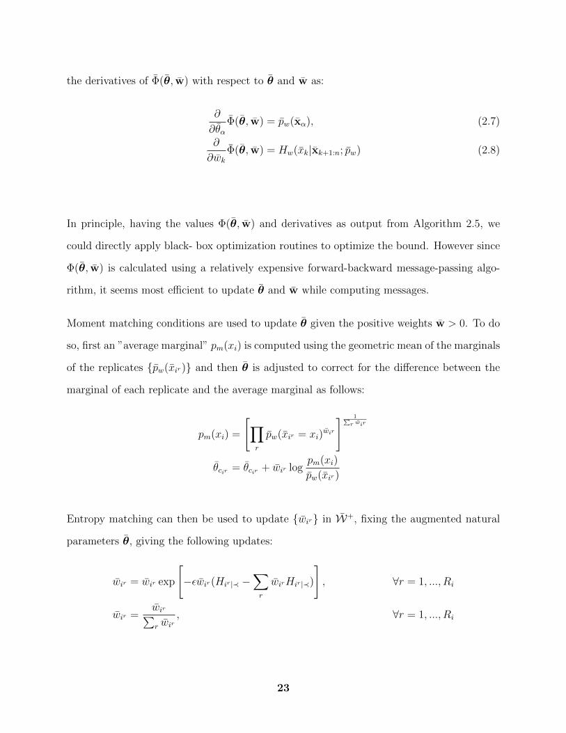
the derivatives of Φ(θ, w) with respect to θ and w as:
∂
∂θαΦ(θ, w) = pw(xα), (2.7)
∂
∂wkΦ(θ, w) = Hw(xk|xk+1:n; pw) (2.8)
In principle, having the values Φ(θ, w) and derivatives as output from Algorithm 2.5, we
could directly apply black- box optimization routines to optimize the bound. However since
Φ(θ, w) is calculated using a relatively expensive forward-backward message-passing algo-
rithm, it seems most efficient to update θ and w while computing messages.
Moment matching conditions are used to update θ given the positive weights w > 0. To do
so, first an ”average marginal” pm(xi) is computed using the geometric mean of the marginals
of the replicates {pw(xir)} and then θ is adjusted to correct for the difference between the
marginal of each replicate and the average marginal as follows:
pm(xi) =
[∏r
pw(xir = xi)wir
] 1∑r wir
θcir = θcir + wir logpm(xi)
pw(xir)
Entropy matching can then be used to update {wir} in W+, fixing the augmented natural
parameters θ, giving the following updates:
wir = wir exp
[−εwir(Hir|≺ −
∑r
wirHir|≺)
], ∀r = 1, ..., Ri
wir =wir∑r wir
, ∀r = 1, ..., Ri
23
Very important aspect of such optimization which directly impacts the tightness of the bound
is the structure of the cluster tree over which the augmented model p(x) is formed. Such
structure can be formed by running the mini-bucket elimination Algorithm 2.3 which requires
partitioning the functions that belong to a bucket into smaller mini-buckets. Different parti-
tioning strategies result in different structures than can affect the tightness of the bound and
have been previously studied for selecting better mini-buckets for MBE algorithm [Rollon
and Dechter, 2010]. In Chapter 3 we study one such partitioning strategy which allows us
to add new regions to the cluster tree G incrementally to achieve tighter bounds.
24
Algorithm 2.5 Calculating the WMB bound Φ(θ, w) and its derivatives [Liu and Ihler,2011]
Input: Set of augmented factors of a graphical model {fck(xck)} and their cluster tree G.A weight vector w = [w1, . . . , wn]. An elimination order o = [11, . . . , 1R1 , . . . , n1, . . . , nRn ]
Output: Φ(θ, w) and its derivativesForward pass:for i← 1 to n do
λi→l(xi→l) =[∑
xi
(fci(xi)∏
j∈child(i)
λj→i(xj→i))1wi
]wiwhere l = πi is the parent of ci and child(i) is the set of nodes that have i as theirparents.
end forBackward pass:for i← n to 1 do
λk→i(xk→i) =[ ∑
xk\xi
(fck(xk)∏j∈δ(i)
λj→i(xj→i))1wi λi→k(xi→k)
− 1wi
]wmiwhere δ(i) is all the nodes connected to i in the cluster tree G including its parent k
end forCompute the bound:
Φ(θ, w) = log∏k
wk∑xk
[fck(xk)∏i∈δ(k)
λi→k(xi→k)]
where k lists all the clusters with no parents in G.Compute the approximate marginals:
pw(xck) ∝ [fck(xk)∏i∈δ(k)
λi→k(xi→k)]1wk
25
2.2 Variational Methods
All inference methods discussed so far use a sequence of variable elimination steps to compute
the partition function. In contrast, variational methods convert the inference problem into
an optimization task over the space of distributions. The goal is then to find a distribution
minimizing a divergence measure to the target distribution over which we can solve the
inference problem more efficiently. To review the variational inference framework next we
introduce the exponential family form for graphical models and the variational form for the
log-partition function.
2.2.1 Exponential Family and Marginal Polytope
The factorized distribution p(x) =1
Z
∏α
fα(xα) can be written into an overcomplete expo-
nential family form [Wainwright and Jordan, 2008b],
p(x;θ) = exp(θ(x)− Φ(θ)) θ(x) =∑α∈I
θα(xα) (2.9)
where θα(xα) = log(fα(xα)) are the log of the factors fα in our graphical model. The values
θα are called the natural parameters of the exponential family and the vector θ = {θα(xα) :
α ∈ I,xα ∈ Xα} is a vector formed by concatenating all the natural parameters. Φ(θ) is
then the log-partition function, that normalizes the distribution
Φ(θ) = log∑
x
exp(θ(x)) (2.10)
The framework of variational inference converts the problem of computing the log-partition
function (2.10) to an optimization problem:
Φ(θ) = maxq∈Px{Eq(θ(x)) +H(x; q)} (2.11)
26
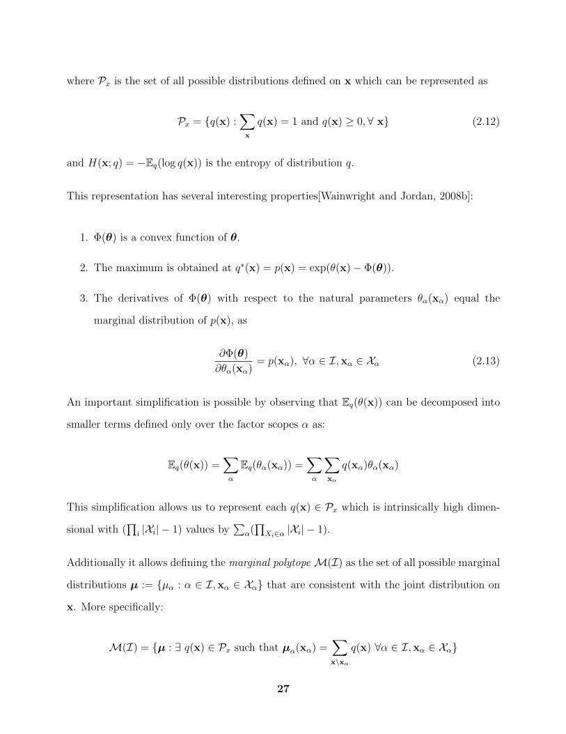
where Px is the set of all possible distributions defined on x which can be represented as
Px = {q(x) :∑
x
q(x) = 1 and q(x) ≥ 0,∀ x} (2.12)
and H(x; q) = −Eq(log q(x)) is the entropy of distribution q.
This representation has several interesting properties[Wainwright and Jordan, 2008b]:
1. Φ(θ) is a convex function of θ.
2. The maximum is obtained at q∗(x) = p(x) = exp(θ(x)− Φ(θ)).
3. The derivatives of Φ(θ) with respect to the natural parameters θα(xα) equal the
marginal distribution of p(x), as
∂Φ(θ)
∂θα(xα)= p(xα), ∀α ∈ I,xα ∈ Xα (2.13)
An important simplification is possible by observing that Eq(θ(x)) can be decomposed into
smaller terms defined only over the factor scopes α as:
Eq(θ(x)) =∑α
Eq(θα(xα)) =∑α
∑xα
q(xα)θα(xα)
This simplification allows us to represent each q(x) ∈ Px which is intrinsically high dimen-
sional with (∏
i |Xi| − 1) values by∑
α(∏
Xi∈α |Xi| − 1).
Additionally it allows defining the marginal polytope M(I) as the set of all possible marginal
distributions µ := {µα : α ∈ I,xα ∈ Xα} that are consistent with the joint distribution on
x. More specifically:
M(I) = {µ : ∃ q(x) ∈ Px such that µα(xα) =∑x\xα
q(x) ∀α ∈ I,xα ∈ Xα}
27
As a result the optimization (2.11) can now be defined as an optimization over the marginal
potytope M(I) as:
Φ(θ) = maxµ∈M(I)
{〈µ,θ〉+H(x;µ)} (2.14)
where 〈µ,θ〉 is the inner product,
〈µ,θ〉 =∑α∈I
∑xα
µ(xα)θα(xα)
As a result both the partition function and marginals can be computed from a single con-
tinuous optimization (2.14) instead of the sum inference task.
Unfortunately, simply casting the log-partition function as an optimization problem does not
cause the computation to be tractable and the optimization in (2.14) remains intractable
for two reasons: (1) the entropy H(x;µ) is intractable to compute in general, and (2) the
marginal polytope, M, is difficult to characterize exactly, requiring an exponential number
of linear constraints in general.
Approximating the variational form (2.14) efficiently then requires three components: (1)
approximating the marginal polytope M ≈ M; (2) approximating the entropy H(x;µ) ≈
H(x;µ); and (3) solving the continuous optimization with those approximations.
As a result, some of the important problems in variational approximations include the se-
lection of an appropriate entropy approximation H, and the choice of regions, or subsets of
variables whose beliefs are represented directly which often affects both the accuracy of H
and the form of the polytope approximation M.
28
2.2.2 WMBE - The Variational View
As described in section 2.1.3, weighted mini-bucket elimination (WMBE) can be used to
compute an upper or lower bound of the log-partition function by passing weighted mes-
sages forward along an elimination order. The weighted summation and Holder’s inequality
were then used to compute its bounds (2.3) and (2.4). Liu and Ihler [2011] show that this
bound can be interpreted from a variational perspective by first approximating the marginal
polytope by a marginal polytope on the cluster tree formed by the partitions and then
bounding the exact entropy using a weighted conditional entropy.
To make this connection clear, note that the process of partitioning the functions assigned
to the mini-buckets can be interpreted as replicating the variables that appear in different
mini-buckets. Let xi = {xri}Rir=1 be the set of Ri copies of variable xi. Also let wi = {wri }
Rir=1
be the corresponding collection of weights for each replicate such that∑Ri
r=1wri = 1. The
sets x = {x1, . . . , xn} and w = {w1, . . . , wn} thus represent the collection of variable copies
and the weights. The elimination order o = [1, . . . , n] on the original variables x can then
be simply extended to the set x as o = [11, . . . , 1R1 , . . . , n1, . . . , nRn ]. Let θ = {θα : α ∈ I}
be the set of factors defined over the set of variable copies x. Such formulation allows, the
primal WMB bound to be
Φ(θ) ≤ Φ(θ, w) = logwm∑xm
· · ·w1∑x1
∏α∈I
exp(θα(xα)) (2.15)
From the variational perspective, the above replaces the marginal polytopeM on the original
variables, with the marginal polytope M on the variable replicates which means the search
for the mean vector µ ∈ M is replaced with searching for some extended mean vector
µ ∈ M. The entropy can be bounded using a weighted sum of the conditional entropies,
29
computed using the marginals µ, on the mini-bucket graph
H(µ) ≤ Hw(µ) =∑i∈o
wiH(xi|xi+1:n; µ) (2.16)
Plugging the approximations to the marginal polytope M and conditional entropy Hw(µ)
in to (2.14) results in the dual WMB bound to the log partition function
Φ(θ) ≤ maxµ∈M{〈µ, θ〉+ Hw(µ)} (2.17)
In principle, we could use a variety of methods to directly optimize (2.17). However, as Liu
and Ihler [2011] show, the primal WMB bound in (2.15) can be optimized efficiently via
simple message passing updates described in Algorithm 2.5 which is the route we follow in
our later experiments involving WMB.
2.2.3 Variational Methods for Maximization
The variational form (2.14) casts the problem of computing the log-partition function as a
continuous optimization problem. A similar representation exists for the maximization tasks
in graphical models as:
Φ(θ) = maxµ∈M(I)
{〈µ,θ〉} (2.18)
which provides a powerful toolkit for the max-inference; a combinatorial optimization prob-
lem. It is interesting to note that the form (2.18) and (2.14) differ only by the addition of
the entropy term in the latter. Intuitively for the maximization we expect the marginals
of the optimal distribution to correspond to a single assignment while for the summation
the entropy term causes the optimal distribution to spread across many high-probability
30
assignment to increase the entropy.
Approximating the marginal polytope M in (2.18) with a more manageable set such as
the local consistency polytope L results in an approximation known as a relaxation of lin-
ear programming relaxation for MAP inference. Many efficient algorithms have been devel-
oped to solve the linear program (2.18), including max-product linear programming (MPLP)
[Globerson and Jaakkola, 2007b] and dual decomposition [Komodakis et al., 2011, Sontag
et al., 2010]. In Chapter 5 we discuss how to use augmented Langrangian methods com-
bined with the Alternating Direction Method of Multipliers to solve this optimization more
efficiently.
31
Chapter 3
Incremental Region Selection for
Mini-bucket Elimination Bounds
3.1 Region Choice for MBE
The popularity of mini-bucket elimination [Dechter and Rish, 2003] (discussed in detail
in Chapter 2) has led to its use in many reasoning tasks; MBE is often used to develop
heuristic functions for search and combinatorial optimization problems [Dechter and Rish,
2003, Kask and Dechter, 2001, Marinescu and Dechter, 2007, Marinescu et al., 2014], as well
as to provide bounds on weighted counting problems such as computing the probability of
evidence in Bayesian networks [Rollon and Dechter, 2010, Liu and Ihler, 2011].
A critical component of the mini-bucket approximation is the set of partitions formed during
the elimination process. By bounding the size of each partition and eliminating within
each separately, MBE ensures that the resulting approximation has bounded computational
complexity, while providing an upper or lower bound. A single control variable, the ibound,
allows the user to easily trade off between accuracy and computational complexity (including
both memory and time). The partitioning of a bucket into mini-buckets of bounded size can
be accomplished in many ways, each resulting in a different accuracy. From the variational
32
perspective, this corresponds to the critical choice of regions in the approximations, defining
which sets of variables will be reasoned about jointly.
Traditionally, MBE is guided only by the graph structure, using a scope-based heuristic
[Dechter and Rish, 2003] to minimize the number of buckets. However, this ignores the
importance of the function values on the bound. More recent extensions such as Rollon
and Dechter [2010] have suggested ways of incorporating the function values into the par-
titioning process, with mixed success. A more bottom-up construction technique is the
relax-compensate-recover (RCR) method of Choi and Darwiche [2010], which constructs a
sequence of mini-bucket-like bounds of increasing complexity.
Variational approaches typically use a greedy, bottom-up approach termed cluster pursuit.
Starting with the smallest possible regions, the bounds are optimized using message passing,
and then new regions are added greedily from an enumerated list of clusters such as triplets
[e.g., Sontag et al., 2008, Komodakis and Paragios, 2008]. This technique is often very
effective if only a few regions can be added, but the sheer number of regions considered often
creates a computational bottleneck and prevents adopting large regions [see, e.g., Batra et al.,
2011].
We propose a hybrid approach that is guided by the graph structure in a manner similar to
the mini-bucket construction, but takes advantage of the iterative optimization and scoring
techniques of cluster pursuit. In practice, we find that our methods work significantly better
than either the partitioning heuristics of Rollon and Dechter [2010], or a pure region pursuit
approach. We also discuss the connections of our work to RCR [Choi and Darwiche, 2010].
We validate our approach with experiments on a wide variety of problems drawn from recent
UAI approximate inference competitions [Elidan et al., 2012].
33
3.1.1 Partitioning Methods
As discussed above, mini-bucket elimination and its weighted variant compute a partitioning
over each bucket Bi to bound the complexity of inference and compute an upper bound on the
partition function Z. However, different partitioning strategies will result in different upper
bounds. Rollon and Dechter [2010] proposed a framework to study different partitioning
heuristics, and compared them with the original scope based heuristic proposed by Dechter
and Rish [1997]. Here we summarize several approaches.
Scope-based Partitions. Proposed by Dechter and Rish [1997], scope-based partitioning is
a simple but effective top-down approach that tries to minimize the number of mini-buckets
in Bi by including as many functions as possible in each mini-bucket qki . To this end, it first
orders the factors in Bi by decreasing number of arguments. Starting from the largest, each
factor fα is then merged with the first available mini-bucket that satisfies the computational
limits, i.e., where |var(f)∪var(qji )| ≤ ibound+1 where var(f) represents the scope of function
f . If there are no mini-buckets available that can include the factor, a new mini-bucket is
created and the scheme continues until all factors are assigned to a mini-bucket.
Scope-based partitioning provides an efficient way to quickly decide which regions to include
in the cluster graph. However, because it relies solely on the function arguments, it ignores
a significant source of information: the functions values themselves.
Consider an example when eliminating variable X1 from a bucket containing four factors,
{f14, f17, f123, f156} with ibound = 3. Suppose that the two functions f123 and f156 return 1
for every assignment to the variables in their scope, i.e. f123 = 1 and f156 = 1. Eliminating
X1 from the bucket without partitioning is then proportional to eliminating X1 from the
34
(a) (b) (c)
Figure 3.1: Comparing approximations. Suppose f123 = f156 = 1; then (a) exact eliminationprovides the same answer as (b) an approximation using three mini-buckets, while (c) thescope-based approximation of two mini-buckets may give a loose upper bound.
product f14f17 as
∑x1
f14f17f123f156 = C ×∑x1
f14f17 (3.1)
Two ways of partitioning these four functions into different mini-buckets are shown in Figure
3.1(b) and (c). Scope-based partitioning aims to minimize the number of mini-buckets, and
so groups the functions into two mini-buckets, {f123, f14} and {f156, f17}. However, another
choice would be to use three partitions {f123}, {f156}, and {f14, f17}. Comparing the results
of elimination from these two partitionings,
∑x1
f17f123 maxx1
f17f156 = C ×
(∑x1
f14 maxx1
f17
)(3.2)
∑x1
f17f14 maxx1
f123 maxx1
f156 = C ×∑x1
f14f17 (3.3)
with the exact elimination (3.1), we can see that the scope-based partitioning results in a
potentially loose upper bound, while eliminating from the three partitions (3.3) provides the
same value as exact elimination. In other words, the particular values of f123 and f156 cause
a partitioning that looks less accurate (three mini-buckets) to actually provide a much more
accurate approximation.
Content-based Partitions. Since looking at function values can help choose better mini-
35
buckets, Rollon and Dechter [2010] explored informed selection of variable groupings into
mini-buckets based on content-based distance functions, and proposed various content-based
partitioning heuristics that seek to find a partitioning that is closest to the true bucket
function, gi =∑
xi
∏α∈Bi fα.
Rollon and Dechter [2010] frame this selection process as an optimization problem,
Q∗ = arg minQ
dist(gQi , gi), (3.4)
where Q = {q1i , . . . , q
pi } is a partitioning of Bi with bounding parameter ibound and
gQi =
p∏j=1
∑xi
∏α∈qji
fα
is the function represented by the partitioning Q. Rollon and Dechter [2010] studied the ef-
fectiveness of several different distance functions across multiple problem instances; however,
no single distance was found to consistently outperform scope-based partitioning.
It is important to note that we can not efficiently compute all possible partitionings and score
them to decide which one to choose, so Rollon and Dechter [2010] proposed a greedy approach
that organizes the space of partitionings into a lattice using the refinement relation between
partitions. Also, in general, computing the distance (3.4) is exponential in the number
of arguments of gi, since we need to measure the distance of the resulting approximation
function gQi relative to the intractably large true function gi. However, for some types of
distance functions like relative error, they show how to derive a local measure that only
requires computing functions in the two candidate mini-buckets to be merged and can be
interpreted as the penalty or error associated with keeping them separated. In this chapter,
we use the ideas presented in [Rollon and Dechter, 2010] and extend them to form a new
hybrid partitioning heuristic.
36
Relax-Compensate-Recover. Choi and Darwiche [2010] indirectly address the problem of
partition selection within their Relax, Compensate and Recover framework, in which certain
equality constraints in the graph are first relaxed in order to reduce the computational
complexity of inference. New auxiliary factors are then introduced to compensate for the
relaxation and enforce a weaker notion of equivalence. The recovery process then aims to
identify those equivalence constraints whose relaxation were most damaging and recover
them. Choi and Darwiche [2010] proposed a number of recovery heuristics, including mutual
information and residual recovery.
3.1.2 Variational bounds.
The variational viewpoint of inference corresponds to optimizing an objective function over a
collection of beliefs that are constrained to lie within the marginal polytope, or set of marginal
probabilities that can be achieved by some joint distribution. Efficient approximations are
developed by relaxing the optimization to enforce only a subset of the constraints – for
example that the beliefs be consistent between overlapping cliques. In the case of the log
partition function, we also approximate the entropy term in the objective; for example, the
weighted mini-bucket bound is:
logZ ≤ maxbα∈L
∑α
Ebα [log fα] +∑i,α
wiαH(xi|xα\i ; bα)
where∑
αwiα = 1 for all i. Like mini-bucket bounds, the quality of variational bounds
depends significantly on the choice of regions, which determine both the constraints that will
be enforced and the form of the entropy approximation. Traditionally, research on variational
approximations for the log partition function has focused more on the optimization of the
bound through message passing than the region selection aspect. Often, regions are chosen
to match the original model factors, and then may be improved using methods like cluster
pursuit, described next.
37
Cluster Pursuit. Sontag et al. [2008] studied the problem of region selection for MAP
inference in the context of cluster-based dual decomposition relaxations. They developed
a bottom-up approach in which regions (typically cycles or triplets) are added incremen-
tally: First, the dual decomposition bound is optimized through message passing. Then, a
pre-defined set of clusters, such as triplets or the faces of a grid, are scored by computing
a lower bound on their potential improvement to the dual objective; the scoring function
used measures the difference between independently maximizing each pairwise factor, ver-
sus jointly maximizing over the triplet. After adding the best-scoring cluster, or a small
number of them, the procedure repeats. Similar cycle repair processes were also proposed
by Komodakis and Paragios [2008] and Werner [2008], and related cluster pursuit methods
have also been applied to summation problems [Welling, 2004, Hazan et al., 2012]. However,
scoring all possible clusters often becomes a computational bottleneck; for example, to make
the process more efficient, Batra et al. [2011] proposed pre-selection heuristics to reduce the
number of clusters considered.
3.2 A Hybrid Approach
To summarize, existing elimination based approaches avoid the space and time complexity
of exact inference by using a top-down partitioning approach that mimics the construction
of a junction tree and allows large regions to be added to the approximation quickly. In
contrast, message passing algorithms often use cluster pursuit methods to select regions, a
bottom-up approach in which a predefined set of clusters (such as triplets) are scored based
on their potential improvement to the bound, and incrementally added.
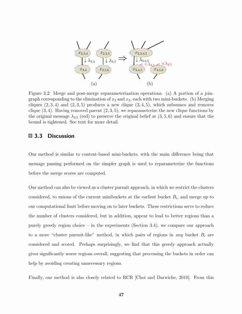
It is important to highlight the relationship between mini-bucket elimination and message
passing, since mini-bucket elimination can be interpreted in the context of cluster graph and
message passing on it. This connection inspires combining message passing techniques with
38
mini-bucket elimination based approximate inference techniques and balance the positive
properties of both. To balance the effectiveness of both approaches, being able to add larger
regions while taking into account their potential improvement to the upper bound for the
log partition function, our hybrid scheme, like mini-bucket, uses the graph structure to
guide region selection, while also taking advantage of the iterative optimization and scoring
techniques of cluster pursuit.
Cluster pursuit algorithms use the function values, and more concretely the improvement
to the bound produced by them, in order to select regions that tighten the upper bound
effectively. However, there are often prohibitively many clusters to consider: for example,
in a fully connected pairwise model, there are O(n3) triplets, O(n4) possible 4-cliques, etc.,
to score at each step. For this reason, cluster pursuit methods typically restrict their search
to a predefined set of clusters, such as triplets [Sontag et al., 2008]. Our proposed approach
uses the graph structure to guide the search for regions, restricting our search to merging
pairs of existing clusters within a single bucket at a time. This allows us to constrain the
complexity of the search and add larger regions more effectively.
In contrast, the content-based heuristics for region selection of Rollon and Dechter [2010]
use the graph structure as a guide, but their scoring scheme only takes into account the
messages from the earlier buckets in the elimination order. Our proposed hybrid approach
uses iterative optimization on the junction tree in order to make more effective partitioning
decisions. Algorithm 3.1 describes the overall scheme of our hybrid approach, which is
explained in detail next.
3.2.1 Initializing a join tree
Given a factor graph G and a bounding parameter ibound, we start by initializing a join
graph, using a min-fill elimination ordering [Dechter, 2003] (which we denote o = {x1, ..., xn}
39
Algorithm 3.1 Incremental region selection for WMBE
Input: factor graph (G), bounding parameter ibound and maximum number of iterationsTInitialize wmb to a join graph using e.g. a min-fill ordering o, uniform weights anduniform messagesfor each bucket Bi following the elimination order do
repeat(qmi , q
ni )← SelectMerge(Qi)
R ← AddRegions(wmb, o, qmi , qni )wmb← MergeRegions(wmb, R)for iter = 1 to T do
without loss of generality) and ibound = 1. For any given bucket Bi, this results in each
mini-bucket (or region) qki ∈ Bi containing a single factor fα. In the sequel, to simplify the
notation, we refer to the mini-bucket qki simply as region k when the context is clear. We
denote the result of the elimination as λk→l and the variables in its scope as var(λk→l). λk→l
is then a message that is sent to the bucket Bj of its first-eliminated argument in o. Here,
l = πk denotes the parent region of k which can be one of the initial mini-buckets in Bj if
var(λk→l) ⊆ var(l), or be a new mini-bucket containing a single factor, fl = 1, that assigns
the value one to every assignment to the variables in var(λk→l). In our implementation we
choose l ∈ Bj to be the mini-bucket with the largest number of arguments, |var(l)|, such
that var(λk→l) ⊆ var(l).
Using the weighted mini-bucket elimination scheme of Algorithm 2.4, we initialize the mini-
bucket weights wr uniformly within each bucket Bi, so that for qri ∈ Qi, wr = 1
|Qi| , which
ensures∑
qri ∈Qiwr = 1.
40
3.2.2 Message Passing
We use iterative message passing on the join graph to guide the region selection decision.
Having built an initial join graph, we use the weighted mini-bucket messages [Liu and Ihler,
2011] to compute forward and backward messages, and perform reparameterization of the
functions fα to tighten the bound.
Let k be a region of the mini-bucket join graph, and l its parent, l = πk, with weights wk
and wl, and fk(xk) the product of factors assigned to region k. xk is then the union of all
the variables in the scope of the factors assigned to region k. Then we compute the forward
messages as,
Forward Messages:
λk→l(xl) =[ ∑
xk\xl
[fk(xk)
∏t:l=πt
λt→l(xl)] 1
wk
]wk(3.5)
and compute the upper bound using the product of forward messages computed at roots of
the join graph,
Upper bound on Z:
Z ≤∏
k:πk=∅
λk→∅ (3.6)
In order to tighten the bound, we compute backward messages in the join graph,
Backward Messages:
λl→k(xk) =[ ∑
xl\xk
[fl(xl)
∏t∈δ(l)
λt→l(xl)] 1
wl[λk→l(xl)
]− 1
wk
]wk
where δ(l) is the set of all neighbors (parent and children) of region l in the cluster tree.
We then use these incoming messages to compute a weighted belief at region k, and repa-
41
rameterize the factors fk for each region k in a given bucket Bi (e.g., k ∈ Qi) to enforce a
weighted moment matching condition:
Reparameterization:
bk(xi) =∑xk\xi
[fk(xk)
∏t∈δ(l)
λt→k(xk)] 1
wk
b(xi) =[ ∏k∈Qi
bk(xi)]1/∑k w
k
fk(xk)← fk(xk)[b(xi)/br(xi)
]wkIn practice, we usually match on the variables present in all mini-buckets k ∈ Qi, e.g.,
∩k∈Qixk, rather than just xi; this gives a tighter bound for the same amount of computation.
3.2.3 Adding new regions
New regions are added to the initial join tree after one or more rounds of iterative optimiza-
tion. To bound the complexity of the search over clusters, we restrict our attention to pairs
of mini-buckets to merge within each bucket and use the elimination order o to guide our
search, processing each bucket Bi one at a time.
Given bucket Bi and a current partitioning Qi = {q1i , ..., q
ki }, we score the merge for each
allowed pair of mini-buckets (qmi , qni ), e.g., those with |var(qmi )∪ var(qni )| ≤ ibound + 1, using
an estimate of the benefit to the bound that may arise from merging the pair:
S(qmi , qni ) = max
xlog [λm→πm(xπm)× λn→πn(xπn)÷ λr→πr(xr)] (3.7)
This score can be justified as a lower bound on the decrease in the approximation to logZ,
since it corresponds to adding region πr with weight wπr = 0, while reparameterizing the
parents πm, πn to preserve their previous beliefs. This procedure leaves the bound unchanged
42
except for the contribution of πr; eliminating with wπr = 0 is equivalent to the max operation.
For convenience, we define S(qmi , qni ) < 0 for pairs which violate the ibound constraint. Then,
having computed the score between all pairs, we choose the pair with maximum score to be
merged into a new clique. In Algorithm 3.1, the function SelectMerge(·) denotes this scoring
and selection process.
3.2.4 Updating graph structure
Having found which mini-buckets to merge, we update the join graph to include the new
clique r = qmi ∪ qni . Our goal is to add the new region in such a way that it affects the scope
of the existing regions in the join tree as little as possible. Adding the new clique is done in
two steps.
First, we initialize a new mini-bucket in Bi with its scope matching, var(r), the scope of
the new merged region r. Eliminating variable xi from this new mini-bucket results in the
message λr→πr . The earliest argument of λr→πr in the elimination order determines the
bucket Bj containing mini-buckets that can potentially be the parent, πr, of the new region.
To find πr in Bj we seek a mini-bucket qkj that can contain r, i.e., var(λr→πr) ⊆ var(qkj ). If
such a mini-bucket exists, we set πr to qkj ; otherwise, we create a new mini-bucket q|Qj |+1j
and add it to Qj, with a scope that matches var(λr→πr). The same procedure is repeated
after eliminating xj from q|Qj |+1j until we either find a mini-bucket already in the join tree
that can serve as the parent, or var(λr→πr) = ∅ in which case the newly added mini-bucket
is a root. Algorithm 3.2 describes these initial structural modifications.
Having added the new regions, we then try to remove any unnecessary mini-buckets, and
update both the join tree and the function values of the newly added regions to ensure that
the bound is improved. To this end, we update every new mini-bucket r that was added
to the join tree in the previous step as follows. For mini-bucket r ∈ Qi, we first find any
43
Algorithm 3.2 AddRegions: find regions to add for merge
Input: The join graph wmb, elimination order o, and mini-buckets qmi and qni to be merged
Output: a list of newly added mini-buckets RInitialize new region qr with var(qr) = var(qmi ∪ qni ) and add it to Qi
repeatUpdate R = R∪ qrSet new clique C = var(qr)\xiif C = ∅ thendone← True
elseFind Bj corresponding to the first un-eliminated variable in C based on eliminationorder ofor each mini-bucket region qkj ∈ Qj do
if C ⊆ var(qkj ) then// forward message fits in existing mini-bucket:done← True
end ifend for
end ifif not done then
// Create a new region to contain forward message:Initialize new region qr with var(qr) = C and add it to Qj
end ifuntil done
mini-buckets s ∈ Qi that can be subsumed by r, i.e., var(s) ⊆ var(r). For each of these
mini-buckets s, we connect all of s’s children (mini-buckets t such that πt = s) to r, e.g., set
πt = r. We also merge the factors associated with r and s, so that fr ← fr × fs.
Next, we reparameterize several other functions in the join graph in order to preserve or
improve the current bound value. Specifically, removing s changes the incoming, forward
messages to its parent, πs = pa(s), which changes the bound. By reparameterizing the factor
at πs,
fπs ← fπs × λs→πs fπr ← fπr ÷ λs→πs
we keep the overall distribution unchanged, but ensure that the bound is strictly decreased.
44
Finally we remove s from Qi, completing the merge of mini-buckets s and r. This process is
given in Algorithm 3.3 and depicted in Figure 3.2 for a small portion of join-graph.
Every merge decision is followed by one or more iterations of message passing, followed
by rescoring the mini-buckets in Bi. The process of message passing and merging continues
until no more mini-buckets of Bi can be merged while still satisfying the bounding parameter
ibound.
Continuing along the elimination order, the same procedure is repeated for the mini-buckets
in each bucket Bi, and the final upper bound to the partition function is computed using
Eq. (3.6).
Computational Complexity of Incremental region selection for WMBE. Rollon and
Dechter [2010] provide an analysis of the computational complexity of their content-based
partitioning heuristic. Following the same framework, next we analyze the computational
complexity of adding new regions in our hybrid approach.
Proposition 3.1. The computational complexity of merging all pair of regions (qm, qn) in
Algorithm 3.1, is at most O( R ·L2 ·exp(z)+R ·L ·z ·exp(z)+T ·R2 ·exp(z) ), where L is the
maximum number of initial regions in a bucket (which can be bounded by the largest degree
of any variable), z is the ibound and R =∑
α |α| bounds the number of possible regions in
the cluster graph.
Proof. Let R be as defined, and denote by O( S ) the computational complexity of a single
merge. There cannot be more than R merges, which means that the complexity of all possible
merges is O(R · S). The complexity of a single merge can then be bounded as O( S ) =
O( L2·exp(z)+L·z·exp(z)+T ·R·exp(z) ). The first term in O( S ) captures the complexity of
computing the score, which is O(exp(z)), for any pair of regions. The algorithm computes the
score for every pair of regions in a bucket, which yields O( L2 ·exp(z) ) for score computation.
45
Algorithm 3.3 MergeRegions: merge and parameterize newly added regions to improvebound
Input: The join graph wmb and a list of newly added mini-buckets Rfor all r ∈ R do
Initialize new region r in Bi with fr(xr) = 1Find regions {s | s ∈ Qi & var(s) ⊆ var(r)}// Remove / merge contained regions s:for all found regions s do
Connect all children of s to rfr = fr × fs // merge factors and// preserve belief at parent πs:fπs = fπs × λs→πsfπr = fπr ÷ λs→πsRemove s from Qi
end forend for
The second term in O( S ) is the complexity bound of the merge process. For each merge we
have to add the new merged region and all its parents, which is bounded by z. After adding
these new regions, we need to check for subsumptions of old regions of the cluster graphs with
the new ones which involves z·L tests. If one region can be subsumed by the other, we need to
update the messages sent to them by their children which requires O( exp(z) ) computations
for each update. Putting it all together, the computational complexity of the merge process
is bounded by O( L · z · exp(z) ). The third component accounts for the complexity of T
iterations of messages passing after each merge, which is bounded by O( T ·R ·exp(z) ) when
we have at most R regions in the cluster graph. Having the complexity of a single merge as
O(S) = O( L2 · exp(z) + L · z · exp(z) + T ·R · exp(z) ), we can then bound the complexity
of doing all merges as O(R ·S) = O( R ·L2 · exp(z) +R ·L · z · exp(z) + T ·R2 · exp(z) ).
46
↓ λ3,4 ↓ λ3,5
x2,3,4 x2,3,5
x3,4 x3,5,6
⇒x2,3,4,5
x3,4,5 x3,5,6
↓ λ3,4,5÷λ3,5 ×λ3,5
(a) (b)
Figure 3.2: Merge and post-merge reparameterization operations. (a) A portion of a join-graph corresponding to the elimination of x2 and x3, each with two mini-buckets. (b) Mergingcliques (2, 3, 4) and (2, 3, 5) produces a new clique (3, 4, 5), which subsumes and removesclique (3, 4). Having removed parent (2, 3, 5), we reparameterize the new clique functions bythe original message λ3,5 (red) to preserve the original belief at (3, 5, 6) and ensure that thebound is tightened. See text for more detail.
3.3 Discussion
Our method is similar to content-based mini-buckets, with the main difference being that
message passing performed on the simpler graph is used to reparameterize the functions
before the merge scores are computed.
Our method can also be viewed as a cluster pursuit approach, in which we restrict the clusters
considered, to unions of the current minibuckets at the earliest bucket Bi, and merge up to
our computational limit before moving on to later buckets. These restrictions serve to reduce
the number of clusters considered, but in addition, appear to lead to better regions than a
purely greedy region choice – in the experiments (Section 3.4), we compare our approach
to a more “cluster pursuit-like” method, in which pairs of regions in any bucket Bi are
considered and scored. Perhaps surprisingly, we find that this greedy approach actually
gives significantly worse regions overall, suggesting that processing the buckets in order can
help by avoiding creating unnecessary regions.
Finally, our method is also closely related to RCR [Choi and Darwiche, 2010]. From this
47
perspective, we “relax” to a low-ibound minibucket, “compensate” by variational message
passing, and “recover” by selecting regions that will tighten the variational bound defined
by the join graph. Compared to RCR, we find a number of differences in our approach: (1)
RCR selects constraints to recover anywhere in the graph, similar to a greedy cluster pursuit;
as noted, this appears to work significantly less well than an ordered recovery process. (2)
RCR makes its recovery updates to the relaxed graph, then (re)builds a (new) join tree over
the relaxed graph; in contrast, we incrementally alter the join graph directly, which avoids
starting from scratch after each merge. (3) Our method is solidly grounded in the theory of
variational bounds and message passing, ensuring that both the message passing and region
merging steps are explicitly tightening the same bound. From this perspective, for example,
it becomes clear that RCR’s “residual recovery” heuristic is unlikely to be effective, since
after message passing, the reparameterization updates should ensure that all mini-buckets
containing a variable xi will match on their marginal beliefs. In other words, residual recovery
is making its structure (region) choices using a criterion that actually measures mismatches
that can be resolved by message passing.
3.4 Empirical Evaluation
To show our method’s effectiveness compared to previous region selection strategies for MBE,
we tested our incremental approach on a number of real world problems drawn from past UAI
approximate inference challenges, including linkage analysis, protein side chain prediction,
and segmentation problems. We compare our hybrid region selection method against the
scope-based heuristic of Dechter and Rish [1997] and the content-based heuristic of Rollon
and Dechter [2010].
48
Table 3.1: UAI Segmentation Instances. Different columns show the bound achievedusing each partitioning heuristic, where “Scp”, “Cont” and “Hyb” represent the naıve scopebased partitioning for MBE [Dechter and Rish, 1997], the context (or energy) based heuristicof Rollon and Dechter [2010] and our hybrid approach interleaving iterative optimization withpartitioning, respectively. In all but one case, our proposed construction provides tighterbounds.
For each set of experiments, we initialize a join tree using WMB elimination with ibound = 1.
We use an elimination ordering found using the min-fill heuristic [Dechter, 2003] and set the
weights uniformly in each bucket. As a result, each mini-bucket qki contains a single factor
fα as described in section 3.2.1.
From this initial setup, we then use Algorithm 3.1 to merge mini-buckets incrementally and
compute the upper bound as in Eq. (3.6).
Segmentation. To evaluate the different methods on pairwise binary problems we used a
set of segmentation models from the UAI08 approximate inference challenge. These models
have ≈ 230 binary variables and ≈ 850 factors. We used varying ibounds for comparison
49
Table 3.2: UAI Pedigree Instances. Different columns show the bound achieved usingeach partitioning heuristic; again, “Scp”, “Cont” and “Hyb” are scope based partitioning[Dechter and Rish, 1997], the content-based heuristic [Rollon and Dechter, 2010] and ourproposed, hybrid approach. In all cases, our proposed construction provides stronger bounds,both before and after full optimization using message passing.
The results show clear improvement in the upper bound using our hybrid approach, indicat-
ing the effectiveness of iterative message passing and optimization in guiding region selection.
To further study the effectiveness of the merged regions in the context of message passing
and optimization, we then fully optimized the join-graphs generated by the three region
50
selection schemes using iterative message passing until convergence. The upper bounds after
this optimization process are denoted by inst-opt for each problem instance, inst. As might
be expected, this additional optimization step improves the bounds of the scope-based and
content-based heuristics more dramatically than our hybrid method; however, even after full
optimization of the bounds, we find that the hybrid method’s bounds remain better in all of
the 6 instances except one, indicating that our method has identified fundamentally better
regions than the previous approaches.
Of course any improvement in the bound from the content-based partitioning and our hybrid
method comes with an additional computational overhead. While our implementations for
these algorithms are in MATLAB and are not optimized for timing experiments, its is im-
portant to consider the effect of this computation on time. In each set of these experiments,
computing the bound using content-based partitioning took on average 10 times more than
scope-based partitioning. Our hybrid approach then requires one round of message passing
after each merge and took on average 10 times more than the content-based to compute the
upperbound.
Linkage Analysis. To compare the various methods on models with non-pairwise factors
and higher cardinalities of variables, we studied pedigree models. The pedigree linkage
analysis models from the UAI08 approximate inference challenge have ≈ 300−1000 variables,
whose cardinalities vary in the range of [2, ..., 5]; the induced width of the models are typically
≈ 20 − 30. We used varying ibounds for comparison and report the results on two values
ibound ∈ [5, 10] .
Table 3.2 shows the upper bounds on a subset of pedigree problems, again showing the
effectiveness of the hybrid method: we find that again, the hybrid method consistently
outperforms the other two region selection approaches, and results in better fully optimized
bounds in all of the 22 instances when ibound = 5 and all but two cases when ibound = 10.
51
ibound
4 6 8 10 12 14 16 18 20
Lo
gZ
up
pe
r b
ou
nd
-90
-85
-80
-75
-70
-65
-60
Scp
Cont
Hyb
Scp-opt
Cont-opt
Hyb-opt
Figure 3.3: The upper bound achieved by the three partitioning heuristics for pedigree23instance over ibound range between 4 to 20.
As for the segmentation instances, computing the upperbound using our hybrid approach is
on average 10 times slower than using the content-based partitioning and using content-based
partitioning is on average 10 times slower than using the scope-based heuristic.
Effect of ibound. We also studied the results of the three partitioning methods across a
range of ibounds, to understand how our method’s effectiveness changes as a function of
the allowed region sizes. Figure 3.3 shows the results for an instance of pedigree dataset.
Empirically, our method is more effective on smaller ibounds, where there are a large number
of possible merges and finding the best one results in a greater improvement to the upper
bound. For larger ibounds, where the resulting cluster trees are relatively close to that of
exact variable elimination, the upper bounds produced by all three heuristics are also fairly
close.
Protein Side-Chain Prediction. Finally, to examine models over high-cardinality variables,
we look at a subset of the protein side chain prediction models, originally from Yanover and
Weiss [2003] and Yanover et al. [2006]. These models contain ≈ 300 − 1000 variables with
cardinalities between 2 and 81, with pairwise potential functions. For these problems, we
only ran our experiments using ibound = 2, due to the high number of states for each variable.
Table 3.3 shows the results of the three partitioning methods, which again agrees with the
52
previous experiments: our hybrid method outperforms the other two in all 44 instances in
the problem set, often dramatically, both before and after the bound is fully optimized.
For these set of instances where the variables have large cardinalities, computing the upper
bound using our hybrid approach is on average 10 times slower than using the content-based
partitioning and using content-based partitioning is on average 20 times slower than using
the scope-based heuristic.
Greedy vs. Elimination Order Based Merging. As discussed before, we restrict the clus-
ters considered for merges to unions of the current minibuckets at the earliest bucket Bi,
and merge up to our computational limit before moving on to later buckets, which serves to
reduce the number of clusters considered. We compare our choice of clusters with a purely
greedy region choice in which pairs of regions in any bucket Bi are considered and scored.
Interestingly, the upper bounds achieved using the greedy approach were not better than the
top-down merging based on elimination order. A possible reason for this behavior is that the
top-down approach allows large regions generated by mini-buckets early in the elimination
ordering to be processed by buckets later in the order; the greedy approach disrupts this flow
and results in extra regions that cannot be merged with any other region while respecting
the ibound.
53
Table 3.3: Protein side-chain prediction. Here we show results for only ibound = 2,due to the high number of states in each variable. Our method often produces dramaticallybetter partitionings than scope- or content-based mini-bucket partitions.
Table 3.4: Top-down vs. Greedy Merging. We examine the effect of using a “fullygreedy” merging procedure closer to standard cluster pursuit, in which we merge the best-scoring cluster in any bucket at each step. We find that following the top-down orderingactually results in significantly better bounds. Results shown are for ibound = 5.
We presented a new merging heuristic for (weighted) mini-bucket elimination that uses mes-
sage passing optimization of the bound, and variational interpretations, in order to construct
a better heuristic for selecting moderate to large regions in an intelligent, energy-based way.
Additionally we showed how to incrementally update the join graph of mini-bucket elimina-
tion after new regions are added in order to avoid starting from scratch after each merge.
Our approach inherits the advantages of both cluster pursuit in variational inference, and
(weighted) mini-bucket elimination perspectives to produce a tight bound. We validated
our approach with experiments on a wide variety of problems drawn from a recent UAI
approximate inference competition. In practice, we find that our methods work significantly
better than either existing partitioning heuristics for mini-bucket [Rollon and Dechter, 2010],
or a pure region pursuit approach. We expect this construction to improve our ability to
search and solve large problems. However, our method does involve additional computational
overhead compared to, say, scope-based constructions, in order to to evaluate and make
merge decisions. We did not focus here on any-time performance; a more nuanced balance
of time, memory, and bound quality is one direction of potential future study.
55
Chapter 4
Improving Resource Usage in
Mini-bucket Elimination
4.1 Introduction
In Chapter 3, we presented an incremental form of mini-bucket elimination (MBE) that
proposed new heuristics for selecting the regions, or mini-buckets, used in the approximation.
As with standard mini-bucket, we used a single control parameter, the ibound, to manage the
computational (time) and representational (memory) complexity of the approximation by
limiting the number of variables in each region. One of the main reasons MBE is so successful
is the easy tradeoff between memory and quality: Using more memory (larger regions) almost
always provides a significant improvement in quality, especially on summation problems (e.g.,
computing the log partition function); see Liu and Ihler [2011].
However, when applying MBE to real-world problems, we need to run it on a wide array of
problem types with very different properties, in terms of graph structures and cardinalities of
variables. Consider an example of protein side-chain prediction, where the model is dense and
pairwise, on perhaps 350 variables with cardinalities that vary between 2 and 81; choosing an
ibound = 4 for MBE with scope-based partitioning requires 17 GB of memory. In contrast,
56
for a linkage analysis (pedigree) instance, the graph is relatively sparse, and the 448 variables
have cardinalities that vary between 2 and 5, and we can compute an approximation with
ibound = 16 and using only 1 GB of memory. As a result, to be able to apply MBE to these
different problems, we need robust methods that can find good approximations in the face
of this kind of diversity.
A central challenge is then to automatically and quickly build approximations that satisfy
the resource constraints, and in particular the amount of memory available. As we discuss in
Section 4.2, finding the largest ibound that respects the memory limits is easy and efficient
for scope-based heuristics. However, for content-based heuristics, the regions are selected
based on the values of the functions and the incoming messages, which means that the exact
memory requirement of a particular execution is not easily evaluated without fully computing
the bound. If the resulting approximation uses too much memory, this work is wasted; if we
have memory left over, we may need to repeat the effort. For this reason, it would be useful
to be able to estimate and control the amount of memory used by an approximation on the
fly, as it is built.
In this chapter we first review the state of the art and discuss the challenges of estimating
the memory needs of content-based MBE. Then we propose two improvements that allow
us to better control how limited memory resources are used, and as a result often provide a
better bound on the partition function. Our goal is to more fully utilize the available memory
resources, while also allowing us to also use content-based selection methods that typically
give tighter bounds. We evaluate our framework on various real world problems and compare
different memory management strategies within content-based mini-bucket approximation.
57
4.2 State of the Art
In this section, we study the role that limited memory resources play during the design of
a mini-bucket based inference approximation and how current systems address the memory
allocation problem. Memory limits are a common and important form of constraint placed
on approximations; typically, the more memory is available, the better the approximation
quality.
One advantage of scope-based mini-bucket elimination is that it is relatively easy to design
an approximation that can fit in the available memory. For scope-based partitions, the
elimination process can be simulated very quickly for various ibound values. Using the
scopes of the intermediate functions, but without actually computing any of the functions
themselves, one can quickly compute the used memory, and select the largest ibound that
complies with the memory constraints; see Otten et al. [2012] for an example. Also, since
the amount of memory grows exponentially as ibound is increased, it is easy to search over
different values of ibound as the range of values in the search space is relatively small.
However, using the scope-based simulation with a particular ibound value to estimate the
memory required by an approximation has two main disadvantages, discussed next.
4.2.1 Content-based region choices
For content-based mini-bucket, ensuring bounded memory use by searching over ibound is
not as easy as scope-based mini-bucket elimination. In particular, the partitioning process
depends on the values of the functions and incoming messages, which means that it cannot
be simulated without fully computing the functions and messages.
From this perspective, an incremental approach (e.g., the method described in Chapter 3)
is a useful paradigm. However several issues should be addressed. For example, in Chapter
58
3 we showed that it was best to do all merges within a single bucket before moving on to
a later bucket. However, allowing all the memory to be used by the earlier buckets in the
elimination order is unlikely to be an effective use of the available memory. This suggests
that some “forecasting” of memory use in future buckets is probably useful.
A possibly naive way to estimate the amount of memory required by the content-based parti-
tioning process is to compute the amount of memory required by the scope-based mini-bucket
and use it as an estimate for the memory used by the content-based process. However for
models with even moderate variation in the domain size of the variables, different partitioning
choices can result in very different memory use. Then, when processing for a given ibound,
if the available memory is exceeded the procedure will not provide a usable approximation;
if it uses less memory than is available, it may result in a poor quality one.
Figure 4.1 (a) shows an example of this difference in memory use for protein side-chain
prediction instances, where WMBE is used to compute an upper bound to the log partition
function with ibound = 2, using scope- and content-based heuristics. The memory required
by the content-based approximation is compared to the memory required by the scope-based
approximation by computing the difference, (M(Ctnt)−M(Scp)) /M(Scp). Here M(Ctnt)
is the memory required by the content-based partitioning andM(Scp) is the memory required
by scope-based partitioning. For some instances, the content-based partitioning required
more memory than scope-based, while for the others, the relationship is reversed. This
property makes it difficult to use the scope-based ibound value, and its associated memory
use, as an accurate estimate for a content-based partitioning. Hence we would like an
“online”, memory-aware partitioning procedure that can estimate and manage the amount
of memory it requires while building the approximation.
59
1c4o
1e18
1ddt
1nr0
1tyv
1qpk
1cb6
1l2q
1qcf
1ug6
1kw
h
1n5u
2nap
1eu8
-0.2
0
0.2
0.4
0.6
0.8(
M(C
tnt)
- M
(Scp
) )
/ M(S
cp)
1ju3
1eu8
1f5n
1n5u
1cb6
2nap
1exm
1e4f
1gsk
1fs7
1qpk
1dpe
1crz
1jy1
0
20
40
60
80
100
% M
emor
y U
sed
(a) (b)
Figure 4.1: (a) Memory used by content-based partitioning, compared to the memory usedby scope-based partitioning in WMBE. Different partitioning decisions can lead to sig-nificantly varying memory requirements. We show the relative difference in memory use,M(Ctnt)−M(Scp)
M(Scp), across several problem instances, where M(Ctnt) is the memory required by
weighted mini-bucket elimination using content-based partitioning and M(Scp) is the mem-ory required by scope-based partitioning. Positive values indicate the content-based parti-tioning required more memory. (b) Percentage of memory used by scope-based mini-bucketelimination when the ibound parameter is set to the largest value for which the mini-bucketcluster tree fits in memory, across several protein examples. For many instances, a largefraction of the available memory is left unused.
4.2.2 Inefficient memory allocation
Another aspect of estimating the required memory for any mini-bucket approximation is the
relationship between ibound and the memory required by the resulting mini-bucket approxi-
mation. Standard practice finds an ibound such that MBE using ibound+1 does not fit in the
memory. However, the ibound is a very coarse mechanism for controlling how much memory
is used, as any change in the ibound changes the amount of required memory exponentially.
This exponential growth makes searching over ibound values efficient, but also means that
the approximation built with the largest ibound may use only a fraction of the available
memory. This effect is more pronounced in models with larger domain sizes of the variables.
Figure 4.1 (b) shows this effect for instances of protein side-chain prediction problems. Each
bar shows the percent of memory used by scope-based mini-bucket elimination when ibound
is set to the largest value for which the cluster tree fits in memory. For many instances, a
large fraction of the available memory is unused. This effect argues for a more fine-grained
approach, or possibly a coarse-to-fine memory allocation procedure. Again, forecasting the
60
memory requirements for an approximation as new regions are added to the approximation
would be useful, as some buckets could use higher ibound values than others if we can afford
it.
To this end, we propose a set of budget-based memory allocation strategies that allow finer
control over how the available memory is used. We frame these approaches in terms of
the basic incremental cluster tree construction proposed in Chapter 3, then propose and
study empirically several mechanisms for setting the initial budget values, and updating the
budgets as the cluster tree is built.
4.3 Memory awareness
A key component of our framework is the incremental perspective to adding new regions;
to this end we will rephrase existing elimination based methods within our incremental
viewpoint. First, we define some of the the notation that we will require throughout the
chapter.
Let wmb be a valid mini-bucket cluster tree for a graphical model consisting of variables
X = {X1, . . . , Xn} and factors F = {fα(Xα)}, indexed by their scopes α ⊆ {1, . . . , n}, with
respect to ordering o = [X1, . . . , Xn]. Then, wmb consists of a set of regions (or mini-buckets)
R organized into buckets B1, . . . , Bn, with the properties:
1. Each factor fα can be assigned to a region that contains its scope:
∀α, ∃r ∈ R s.t. Xα ⊆ var(r)
where var(r) is the set of variables in region r.
2. Each region r ∈ R is associated with the bucket corresponding to its earliest eliminated
61
variable,
r ∈ Bi iff Xi ∈ var(r) and ∀Xj ∈ var(r), j ≥ i
where j ≥ i means that Xj is eliminated later than Xi in ordering o.
3. Each region r with more than one variable is identified with a parent region πr to which
its downward message (eliminating Xi) can be assigned:
if |var(r)| > 1 and r ∈ Bi, ∃πr ∈ R with var(r) \Xi ⊆ var(πr)
Now, we define several useful functions for measuring the computational resources associated
with the cluster tree wmb, bucket Bi, or region r:
size(r) = |var(r)| : the number of variables in region r
size(Bi) = maxr∈Bi
size(r) : the size of the largest region in Bi
size(wmb) = maxisize(Bi) : the size of the largest region in R
M(r) =∏
Xi∈var(r)
|Xi| : the number of entries in a table over the variables in r
M(Bi) =∑r∈Bi
M(r) : the total number of entries in the tables for regions in bucket i
M(wmb) =∑i
M(Bi) : the total number of entries in all tables for the regions in R
Then, “size(·)” corresponds to measuring the inherent complexity or memory requirements
of a region, bucket, or cluster tree according to its scope (as is typical for standard mini-
bucket formulations), while “M(·)” corresponds to measuring its complexity in terms of the
amount of memory required to represent an arbitrary function over those variables. We also
define the total memory budget (the memory available for inference) as M.
Two key steps of the incremental perspective are: (1) forming the initial cluster tree, and
62
(2) merging new regions and updating the graph structure.
Initializing the cluster tree. Given the factor graph G, our incremental approach starts
from an “initial” cluster tree, where each factor is a region, with descendants corresponding
to partial eliminations of that factor. We construct this initial cluster tree, wmb, using a
min-fill elimination ordering o and ibound = 1. For any given bucket Bi, this results in
each mini-bucket (region) r ∈ Bi containing a single factor. We represent the result of
the elimination as as message, λr→πr , with scope var(λr→πr), from region r to its parent
πr in a later bucket Bj, corresponding to its first-eliminated argument in o. The parent
region πr may be one of the initial mini-buckets in Bj, if a region in Bj with sufficient scope
already exists, or be a new mini-bucket. In our implementation we choose πr ∈ Bj to be
the mini-bucket over the most variables, such that var(λr→πr) ⊆ var(πr). To enable memory
awareness we also evaluate M(r) and M(Bi) for every region r and bucket Bi in the initial
cluster tree to keep track of the memory used.
Merge Operation. Algorithm 4.1 is used to score pairs of regions in each bucket and to
select the best region to be added to the current cluster tree based on a predefined scoring
function. Having selected which two regions to merge, we can then use the subroutines
AddRegion(.) (Algorithm 3.2) and MergeRegions(.) (Algorithm 3.3) defined in Chaper 3
to add the new region to the cluster tree. However, to be memory-aware, we need to check
if the updated cluster tree after the merge still respects the memory limit M. To do so,
SelectMerge(.) simulates the process of adding the newly merged region and computes the
additional memory required by the merge. This additional memory accounts for adding the
new regions to the cluster tree wmb and updating its structure. To do so, Algorithm 4.1
first simulates the merge process using Algorithm 4.6 and scores pairs of mini-buckets only
if the resulting cluster tree can still fit in the available memory.
To simulate the process of merging regions rj and rk in bucket Bi and adding the new region
63
Algorithm 4.1 SelectMerge: Scoring all possible merges in a bucket while taking intoaccount the total memory M
Input: cluster tree wmb, bucket Bi, elimination order o, total memory available Mfor every pair (rj, rk) in Bi such that |var(rj) ∪ var(rk)| < ibound + 1 do
// check if merge respects the memory budget :Let C = var(rj) ∪ var(rk) be a clique containing all variables from rj and rkMnew ← CheckMem(wmb, o, C, M)if Mnew <M thenS(j, k)← score(rj, rk)
elseS(j, k)← − inf
end ifend for// select the best merge:(j∗, k∗) = arg maxj,k S(j, k)Return: (rj∗ , rk∗)
rn, Algorithm 4.6 uses the clique C = var(rj) ∪ var(rk), which contains the variables in the
two regions rj and rk. The newly merged region rn then has C as its scope. The memory
required by bucket Bi after the merge, Mnew(Bi), is updated to account for the new region.
To do so, the memory required by the new region, M(rn), is added to the current amount
of memory used by Bi, M(Bi). The process also checks for any other regions in bucket Bi
that can be subsumed by the new region rn during the merge, and adds the memory used by
those to Mold. To account for the memory that is going to be available when these regions
are subsumed by rn, Mold is then subtracted from Mnew. The total memory required by
the cluster tree after adding this new region to bucket Bi is then updated in Mused and is
compared with the total available memoryM. If the new region can be added, we then need
to account for the memory required for updating the cluster tree structure. Eliminating
variable Xi from the new region rn results in a message λr→πr which has C = C\Xi as its
scope. This message is sent to the bucket Bm corresponding to the first variable of C in the
elimination order. If Bm has any region, rk, that can subsume the message ( e.g. C ⊆ var(rk)
), then no new regions need to be added to the cluster tree. If it can not be subsumed, then
a new region rn should be added to the cluster tree and the memory required for it should
64
Algorithm 4.2 WMBE-IB: Memory-aware Incremental region selection for WMBE usingibound
Input: factor graph (G), ibound, and the available memory MInitialize wmb to a cluster tree using e.g. a min-fill ordering o, uniform weights// pass forward messages along the elimination orderwmb← msgForward(wmb)for each bucket Bi following the elimination order do
repeat(rm, rn)← SelectMerge(Bi, ibound, M)R ← AddRegions(wmb, o, rm, rn)wmb← MergeRegions(wmb, R)// pass forward messages along the merge path R until we reach a rootset r and πr to the first and second regions in R (πr is parent of r in cluster tree)while πr 6= ∅ do
// pass forward message
λr→πr(xπr) =[∑
xr\xπr
[fr(xr)
∏t:πr=πt
λt→πr(xπr)] 1wπr
]wπrend while
until no more merges possibleend forReturn: Upper bound on Z: Z =
∏r:πr=∅ λr→∅
be added to Mused. This process continues until either the message can be subsumed by a
region that is already in the cluster tree or C\Xm is empty which means that the previously
added region has no parents. Algorithm 4.6 shows details of this process and returns the
total memory required to add the new region rn to the current cluster tree wmb.
4.3.1 Baseline Methods
Having a scoring and merge process that takes into account the memory constraints, we
can now give the basic weighted mini-bucket algorithms in our incremental, memory-aware
framework, detailed in Algorithm 4.2. The scoring function to choose the pair of regions to
add then depends on the partitioning heuristic. For scope based partitioning, we can define,
S(rm, rn) = |var(rm) ∪ var(rn)|,
65
that computes the number of variables in the resulting merged region and for content based
partitioning we can use the scoring function (3.7), defined in Chapter 3.
Computational Complexity of WMBE-IB. As in Rollon and Dechter [2010] next we an-
alyze the computational complexity of adding new regions using our incremental memory-
aware approach.
Proposition 4.1. The computational complexity of merging all mergable pairs of regions
(rm, rn) in WMBE-IB (Algorithm 4.2), is at most O( R · L2 · exp(z) +R · L3 · z +R · L · z ·
exp(z)+R ·n ·exp(z) ), where L is the maximum number of initial regions in a bucket (which
can be bounded by the maximum degree of any variable), z is the ibound, n is the number of
variables in the graphical model and R =∑
α |α| upper bounds the maximum possible regions
in the cluster graph.
Proof. Let R be as defined, and denote by O( S ) the computational complexity of a single
merge. We cannot make more than R merges, which means that the complexity of all
possible merges is O(R · S). The complexity of a single merge can then be bounded as
O( S ) = O( L2 ·exp(z)+L3 ·z+L ·z ·exp(z)+n ·exp(z) ). The first term in O( S ) captures
the complexity of computing the score, which is O(exp(z)), for any pair of regions. The
algorithm computes the score for every pair of regions in a bucket, which yields O( L2·exp(z) )
for score computation. The second term in O( S ) is the complexity of CheckMem(.) that
simulates the merge process to decide if a merge fits in memory. For each merge we have
to add the new merged region and all its parents, which is bounded by z. After adding
these new regions, we need to check for subsumptions of old regions of the cluster graphs
with the new ones which involves z · L tests. Checking for the required memory using
CheckMem(.) should be done for all merges in the bucket, and results in total computational
complexity of O( L3 · z ). The third term then computes the bound for updating the
graph structure for the pair that is selected to be merged. As before the complexity of
66
adding the new merged region and its parents is bounded by z, with z · L possible merges
between the old regions and the new ones. For every such merge, if one region can be
subsumed by the other, we need to update the messages sent to them by their children
which requires O( exp(z) ) computations for each update. Putting it all together, the
computational complexity of the merge process is bounded by O( L · z · exp(z) ). Having
updated the cluster graph structure, the complexity of computing the messages from the
newly added region to the root is bounded by n · exp(z). Having the complexity of a single
merge as O(S) = O( L2 · exp(z) +L3 · z+L · z · exp(z) +n · exp(z) ), we can then bound the
complexity of doing all merges as O( R·L2·exp(z)+R·L3·z+R·L·z·exp(z)+R·n·exp(z) ).
This memory-aware incremental built have several advantages: (1) It allows assessing the
memory required for each new region, and only adds those regions that result in an updated
cluster tree that still fits in the available memory. As a result, the algorithm never runs
out of memory, merging as many regions as possible along the elimination order, and always
produces an upper bound. (2) When the ibound found by simulating the scope-based parti-
tioning for mini-bucket elimination leaves a large portion of memory unused, we can use the
memory-aware incremental region selection of Algorithm 4.2, WMBE-IB, with ibound+1 and
allow it to use as much memory until it cannot add any new regions to the approximation.
We will study this memory allocation strategy empirically in section 4.4.1.
However, using a larger ibound to compensate for the large amount of unused memory is not
the only possible solution. In the next section we define the concept of “memory budget”
which allows us to have finer control over how the available memory is used by different
buckets, and describe how the memory-aware algorithm 4.2 can be updated to use the
memory budget instead of a fixed ibound.
67
4.3.2 Memory Budget for Weighted MBE
Given a graphical model and a fixed memory limit M, our goal is to define and evaluate
several different online memory allocation schemes that allow us to have finer control over
how the available memory is used. We would like to be able to use the available memory as
efficiently as possible and achieve tight approximations.
To do so we define the memory budget for bucket Bi, MB(Bi), as the amount of memory
allocated to bucket Bi which can be used by all the mini-buckets included in that bucket.
This means that∑
r∈BiM(r) ≤ MB(Bi) should hold for every bucket Bi. We represent
the memory budget for the cluster tree wmb as MB(wmb) = {MB(Bi) for Bi ∈ wmb}.
The total memory available is then distributed between different buckets such that M =∑Bi∈wmbMB(Bi).
The memory budget for bucket Bi can then replace the fix ibound to control the amount of
memory used by Bi. A memory allocation scheme then defines how the available memory,
M, should be distributed among different buckets along the elimination order. There are two
questions that need to be addressed by each memory allocation scheme; 1) How to initialize
the memory budget for each bucket and 2) how to update the initial estimate as we merge
mini-buckets using different partitioning schemes.
However, in order to use any memory allocation scheme, we need to be able to keep track
of the available memory and the memory used by different mini-buckets as we add more
regions to mini-bucket approximation. To do so, we modify Algorithm 4.2, to use a memory
budget instead of ibound. Algorithm 4.3 shows the details of memory-aware incremental
region selection using memory budget. The general procedure to select and add regions is
as before, when using ibound and total available memoryM. The only difference is that the
new procedure keeps track of the memory budget and how it is used at each bucket, which
is explained in detail next.
68
Algorithm 4.3 WMBE-MB: Memory-aware Incremental region selection for WMBE usingmemory budget
Input: factor graph (G), available memory MInitialize wmb to a cluster tree using e.g. a min-fill ordering o, uniform weights// pass forward messages along the elimination orderwmb← msgForward(wmb)Initialize Memory Budget MB(wmb)← InitMB(wmb)for each bucket Bi following the elimination order do
repeat(rm, rn,M(rm, rn))← SelectMergeMB(Bi, MB(wmb))R ← AddRegions(wmb, o, rm, rn)wmb← MergeRegions(wmb, R)// pass forward messages along the merge path R until we reach a rootset r and πr to the first and second regions in R (πr is parent of r in cluster tree)while πr 6= ∅ do
// pass forward message
λr→πr(xπr) =[∑
xr\xπr
[fr(xr)
∏t:πr=πt
λt→πr(xπr)] 1wπr
]wπrend while// update available memory :MB(wmb)← UpdateBudgetMerge(MB(wmb),M(rm, rn) )
until no more merges possible// update available memory :MB(wmb)← UpdateBudget(MB(wmb))
end forReturn: Upper bound on Z: Z =
∏r:πr=∅ λr→∅
Initialization. Given the factor graph G and the elimination order o, as before, first we
initialize a cluster tree wmb with ibound = 1. Next, we initialize a memory budget MB(wmb)
to manage memory allocation and keep track of the memory used as new regions are added
to the approximation. To do so, taking into account the amount of memory used by the
initial cluster tree, M(wmb), the available memory is updated asM =M−∑
Bi∈wmbM(Bi)
and the memory budget MB(wmb) is initialized by distributing available memory among
different buckets based on a memory allocation scheme (described in section 4.3.3). This
step is done by InitMB(wmb) in Algorithm 4.3.
69
Algorithm 4.4 SelectMergeMB: Scoring all possible merges in a bucket while taking thememory budget into account
Input: cluster tree wmb, bucket Bi, elimination order o, memory budget MB(wmb)for every pair (rj, rk) in Bi do
Set C = var(rj) ∪ var(rk) to a clique that contains all variables from rj and rk// check if merge respects the memory budget :(fits,M(rm, rn))← CheckMemMB(wmb,C,MB(wmb))if fits thenS(j, k)← score(rj, rk)// keep track of the memory it requiresM(j, k)←M(rj, rn)
elseS(j, k)← − inf
end ifend for// select the best merge:(j∗, k∗) = arg maxj,k S(j, k)Return: (rj∗ , rk∗) and the corresponding memory profile M(rj∗ , rk∗)
Algorithm 4.5 UpdateBudgetMerge: Updating memory budget after merging (rm, rn)
Input: memory budget MB(wmb), memory profile of the merge M(rm, rn)// compute the extra memory we have along the merge path Bm :ME =
∑Bm
MB(rm, rn)// update the budget along the merge path Bm :for Bi ∈ Bm(end : −1 : 1) do
if MB(Bi) < M(Bi) thenMB(Bi) = M(Bi)
end ifME = ME −MB(Bi))
end forMB(B1) = ME
Selecting Mini-buckets to Merge. To select the pair of mini-buckets to merge, our budget
based algorithm needs to compare the required memory for the merge at each bucket with
the memory budget allocated to them. We update the two subroutines, SelectMerge(.)
and CheckMem(.), to use the memory budget. The updated subroutine, SelectMergeMB(.),
Algorithm 4.4, then uses CheckMemMB(.), Algorithm 4.7, to compute the memory required
for the merge and score the pairs that can be successfully added to the current cluster tree
wmb. Having a memory budget MB(wmb), which defines a limit on how much memory can
70
be used in each bucket, CheckMemMB(.) needs to check if the pair of regions (rm, rn) can be
successfully added to the current cluster tree while respecting the memory budget MB(Bi)
at every bucket that is affected by the merge. The pair is then scored only if it respects the
budget. After scoring all pairs that respect the memory budget, the best is selected to be
added as the next region to the cluster tree.
Checking Memory Requirement of a Merge. Checking for the memory required by a
merge is done by simulating the process of adding the new merged region to the current
cluster tree wmb. If a merge is possible, the subroutine CheckMemMB(.) returns a memory
profile, M(C), for the merge which contains the memory required at each bucket, M(Bi),
that is affected by the merge and contains the amount of memory used by that bucket after
the merge. Algorithm 4.7 details all the steps involved.
The procedure to compute the memory required at each bucket, Mnew(Bi), is similar to
WMBE-IB. However instead of comparing the total memory used after adding the new
regions (Mused) with the total memory available (M) the algorithm compares the memory
used at each bucket (M(Bi)) with the memory budget allocated to it (MB(Bi)). To do so,
when merging the two regions rj and rk into the new region rn, the algorithm first checks if
the required memory at Bi after the merge, Mnew(Bi), respects the memory budget MB(Bi)
and continues only if the required memory is less than the available budget for the bucket.
Adding the new region rn to the cluster tree might require adding additional regions to the
buckets later in the elimination order as well. CheckMemMB(.) keeps track of these buckets
in Bm = {Bi; if ∃ new rn ∈ Bi after the merge}. To decide if there is enough memory for the
merge, the sum of the required memory for all the buckets in Bm is compared with the total
memory available to those by the memory budget, as∑
Bi∈BmMnew(Bi) ≤∑
Bi∈BmMB(Bi).
This comparison assumes that any extra memory that is allocated to the buckets earlier in
the elimination order and is not used, can be shifted to the buckets later in the elimination
71
(a) (b) (c)
Figure 4.2: Updating the memory budget after a merge: (a) Memory budget before merge(b) Memory required by the merge (c) Memory budget after merge
order.
The simulation continues until the new region can be merged with an existing region in the
cluster tree or the new region has no parents. The algorithm then returns if the merge can
be done and the memory required at each bucket Bi ∈ Bm after the merge, in a memory
profile M(C).
Updating graph structure and memory budget. Having selected the two regions to add,
the two subroutines, AddRegions(.) and MergeRegions(.), perform the merge exactly as
before (see Algorithm 3.2 and Algorithm 3.3). After adding the new regions in R to wmb,
WMBE-MB algorithm updates the memory budget for buckets affected by the merge (Bm
in CheckMemMB(.)) before continuing with another round of adding more regions. This
memory budget update is required because CheckMemMB(.) compares the sum of the
required memory for all the buckets in Bm against the total memory available for those by the
memory budget, e.g.∑
Bi∈BmMnew(Bi) ≤∑
Bi∈BmMB(Bi), to decide if a merge is possible.
This comparison is based on the assumption that any amount of available memory can be
shifted to later buckets along the elimination order. As a result a merge can be approved if∑Bi∈BmMnew(Bi) ≤
∑Bi∈BmMB(Bi) while the required memory at some bucket Bj ∈ Bm
is larger than the memory budget at that bucket, e.g. Mnew(Bj) > MB(Bj). Figure 4.2
shows such an example where (a) is the memory budget assigned to the three buckets before
the merge, (b) is the required memory at each bucket for the merged region to be added
to the cluster tree and (c) is the updated memory budget for the three buckets after the
72
merge. The required memory at bucket B2 is more than what is available in the memory
budget, MB(B2), but since bucket B1 has some extra memory that is not used after adding
the new region, a portion of it can be shifted to bucket B2 to make the merge possible.
UpdateBudgetMerge(.), Algorithm 4.5, makes sure that the memory budget after the merge
reflects the actual available memory in each bucket after the merge is done by shifting the
available memory along the elimination order, from buckets with extra memory to those that
require more.
Memory Reallocation. After all possible merges are done for bucket Bi, UpdateBudget(.)
shifts all the unused memory that was assigned to Bi to the buckets later in the elimina-
tion order. This final memory budget update is required only for some memory allocation
schemes, but results in better memory use and a better approximation in all. Section 4.3.3
describes different strategies for reallocating the unused memory.
Computational Complexity of WMBE-MB. Next we analyze the computational com-
plexity of adding new regions using our budget based incremental memory-aware approach.
Proposition 4.2. The computational complexity of merging all mergable pairs of regions
(rm, rn) in WMBE-MB (Algorithm 4.3), is at most O( R · L2 ·M + R · L3 · logM + R · L ·
M · logM + R ·M ), where L is the maximum number of initial regions in a bucket (which
is bounded by the maximum degree of any variable), M is the total memory and R =∑
α |α|
upper bounds the number of regions in the cluster graph.
Proof. Let R be as defined and denote by O( S ) the computational complexity of a single
merge. Again, we cannot have more than R merges, which means that the complexity of
all possible merges is O(R · S). The complexity of a single merge can then be bounded as
O( S ) = O( L2 ·M +L3 · logM +L ·M · logM +M ). The first term in O( S ) captures the
complexity of computing the score, which is O( M ), for any pair of regions. The algorithm
73
computes the score for every pair of regions in a bucket, which yields O( L2 ·M ) for score
computation. The second term in O( S ) is the complexity complexity of CheckMem(.) that
simulates the merge process to decide if a merge fits in memory. For each merge we have
to add the new merged region and all its parents, which is bounded by logM . After adding
these new regions, we need to check for subsumptions of old regions of the cluster graphs
with the new ones which involves logM · L tests. Checking for the required memory using
CheckMem(.) should be done for all merges in the bucket, and results in total complexity of
O(L3 · logM). The third term then computes the bound for updating the graph structure
for the pair that is selected to be merged. Since each elimination reduces the table size
geometrically, the complexity of adding the new merged region and its parents is bounded
by logM , with logM ·L possible merges between the old regions and the new ones. For every
such merge, if one region can be subsumed by the other, we need to update the messages sent
to them by their children; this requires O( M ) computations for each update. Putting it all
together, the computational complexity of the merge process is bounded by O( L·M ·logM ).
Having updated the cluster graph structure, the complexity of computing the messages from
the newly added region to the root is bounded by M . Having the complexity of a single
merge as O(S) = O( L2 ·M + L3 · logM + L ·M · logM + M ), we can then bound the
complexity of doing all merges as O( R ·L2 ·M+R ·L3 · logM+R ·L ·M · logM+R ·M ).
4.3.3 Memory Allocation Schemes
Using the above memory aware algorithm, different memory allocation schemes proceed by
using different methods to initialize the memory budget and update it at each step. Different
schemes studied in this thesis are as follows:
Waterfall Memory Distribution. Perhaps the simplest way to allocate available memory is
to allow each bucket to use as much memory as it needs, adding the largest regions possible to
74
(a) (b) (c)
Figure 4.3: Different memory allocation schemes: (a) Waterfall Distribution where the totalavailable memory is assigned to the first bucket and any extra memory after all merges ateach bucket is redistributed between the buckets later in the elimination order. (b) UniformDistribution where the total available memory is equally split between different buckets; (c)Proportional Distribution where the total available memory is distributed between differentbuckets proportional to the memory used by scope-based partitioning;
the approximation until no more memory is available. In this scheme, all available memory
is initially allocated to the first bucket; see Figure 4.3 (a). Any memory that is unused by
the first bucket can then be shifted along the elimination order to become available to the
next bucket. For this simple allocation scheme, we can define InitMB(wmb) as:
MB(B1) =M
MB(Bi) = 0 for i = 2 . . . N
To update the memory budget after each bucket is processed, we pass any remaining memory
into the next bucket’s budget, defining UpdateBudget(wmb) as
MB(Bi+1)←MB(Bi+1) + (MB(Bi)−M(Bi))
MB(Bi)←M(Bi)
where Bi+1 is the bucket after Bi in the elimination order. This scheme is efficient in the
sense that almost all available memory will be allocated to some mini-bucket. However, it
will typically result in large regions early in the elimination order, and many small regions
in buckets later in the order, which can lead to poor approximation quality.
75
Uniform Memory Distribution. A simple way to encourage a more equitable distribution
of memory to different buckets is to divide the total memory uniformly among buckets; see
Figure 4.3 (b). More formally, for a graphical model with N variables such allocation uses
an initial memory distribution, InitMB(wmb):
MB(Bi) =MN
for i = 1 . . . N
While this allocation strategy is simple to use, it tends to be very conservative. Some parts
of the model are likely to be less complex than others; empirically, we observe that buckets
early in the elimination order often need less memory compared to buckets later in the order,
which often involve larger regions (a consequence of the graph structure and the elimination
ordering chosen).
As a result, uniform memory distribution may not use the available memory as efficiently
as the waterfall distribution. To some extent, we can remedy this limitation during the
UpdateBudget(.) step by shifting any unused memory from earlier buckets to the later ones,
similarly to the waterfall scheme; strategies for performing such memory shifts are discussed
in the sequel.
Proportional Memory Distribution. A final option is to use information from a “pilot”
estimate of the complexity of different portions of the inference process. Since estimating the
structure, and hence memory requirements of, scope based partitioning is easy and efficient,
we can use this scope-only structure to inform our budgets. After searching for the largest
ibound such that a scope-based partitioning will fit in our total memory, we evaluate the
memory usage of each bucket Bi. Then, we initialize our memory budget proportionally to
these values:
MB(Bi) =Ms(Bi)∑iMs(Bi)
×M,
76
where Ms(Bi) is the memory used by bucket Bi in the scope-based partitioning and M
is our total memory ceiling. The proportional scheme provides a better estimate of the
required memory at each bucket, while assuming that the memory needs of the content-
based partitioning will be similar to that of scope-based partitioning at each level. Figure
4.3 (c) shows an illustration of this allocation scheme.
Memory Reallocation. In all memory allocation schemes discussed above, the resulting
regions in one bucket may use less memory than allocated to that bucket’s budget. This
excess memory can then be redistributed among the later buckets in the elimination order,
in the UpdateBudget(.) step in Algorithm 4.3. The waterfall redistribution, in which any
extra memory is placed in the next bucket, is one such method. Alternatively, however, the
extra memory in each bucket can also be distributed among later buckets in other ways –
for example, uniformly among the later buckets:
MB(Bj)←MB(Bj) + (MB(Bi)−M(Bi))/(N − i) for j > i
or, proportionally to the expected needs of the later buckets:
MB(Bj)←MB(Bj) + (MB(Bi)−M(Bi))MB(Bj)∑j>iMB(Bj)
for j > i
and reduce the “budget” of bucket i to reflect its actual use: MB(Bi) = M(Bi).
Given these various initialization and update methods, we can combine them to generate a
number of different memory allocation strategies:
(1) UF: uniform initial distribution with no reallocation;
77
(2) UU: uniform initial distribution with uniform reallocation;
(3) UP: uniform initial distribution with proportional reallocation;
(4) UW: uniform initial distribution with waterfall reallocation;
(5) PF: proportional initial distribution with no reallocation;
(6) PU: proportional initial distribution with uniform reallocation;
(7) PP: proportional initial distribution with proportional reallocation;
(8) PW: proportional initial distribution with waterfall reallocation;
(9) WW: waterfall initial distribution with waterfall reallocation.
78
Algorithm 4.6 CheckMem: Checks if a new clique C can be added to the current clustertree wmb and returns the memory required for the updated cluster tree after merge
Input: The cluster tree wmb, elimination order o, total memory available M and cliqueCOutput: Mused = M(wmb) after the merge is doneInitialize: Bm to the bucket corresponding to the first un-eliminated variable in C basedon elimination order oInitialize: Xm to the variable that is being eliminated at Bm
Initialize: Mused =∑
iM(Bi) to keep track of the memory used by current cluster treewmbInitialize: done← False;while not done do
Consider new region rn with var(rn) = C and set Mold ← 0Find all regions rm ∈ Bm that can be subsumed by rn ( C ⊆ var(rm) ) and add theirmemory, M(rm), to Mold
Set Mnew = M(Bm) +M(rn)−Mold
Update Mused = Mused −M(Bm) +Mnew
if Mused >M then// memory required to add the new region exceeds memory limit:done← True
end ifif not done then
// Remove Xm from C to get the scope of the outgoing message from the new region:
Set new clique C = var(rn)\Xm
if C = ∅ then// new region rn is a root and has no outgoing messages:done← True
elseFindBm corresponding to the first un-eliminated variable in C based on eliminationorder ofor each mini-bucket region rm ∈ Bm do
if C ⊆ var(rm) then// forward message fits in existing mini-bucket:done← True
end ifend for
end ifend if
end whilereturn Mused
79
Algorithm 4.7 CheckMemMB: Checks if a new clique C can be added to the currentcluster tree wmb under the memory budget MB
Input: The cluster tree wmb, elimination order o, memory budget MB and clique COutput: fits← True if C can be added to wmb, and the memory required for the mergeMCInitialize: Bm = {Bj} to the bucket corresponding to the first un-eliminated variable inC, based on elimination order o and Xj to the variable that is being eliminated at Bj
Initialize: fits← True;Consider new region rn with var(rn) = C and set Mold ← 0Find all mini-bucket region rj ∈ Bj that can be subsumed by rn and add their memoryto Mold
Set Mnew(Bj) = M(Bj) +M(rn)−Mold
if Mnew(Bj) > MB(Bj) thenfits← False // New clique doesn’t fit in the budget for bucket Bj
end ifif fits then
repeatSet new clique C = var(rn)\Xj
if C = ∅ thendone← True
elseFind Bj corresponding to the first un-eliminated variable in C based on eliminationorder o and set Xj to the variable that is being eliminated at Bj
for each mini-bucket region rj ∈ Bj doif C ⊆ var(rj) thendone← True // forward message fits in existing mini-bucket
end ifend for
end ifif not done thenBm ← Bm ∪ {Bj} // New region needs to be added to contain forward messageConsider new region rn with var(rn) = C and set Mold ← 0Find all mini-bucket region rj ∈ Bj that can be subsumed by rn and add theirmemory to Mold
Set Mnew(Bj) = M(Bj) +M(rn)−Mold
if∑
Bi∈BmMnew(Bi) >∑
Bi∈BmMB(Bi) then// Total budget along these buckets is not enough to add the new clique Bj:fits← False and done← True
end ifend if
until doneend ifreturn (fits,M(C) = {Mnew(Bi) for Bi ∈ Bm})
80
4.4 Empirical Evaluation
In this section, we compare the proposed memory allocation schemes on two domains of
problems, linkage analysis and protein side chain prediction, from past UAI approximate
inference challenges and study their ability to effectively use the available memory, and
the quality of the bounds they produce on the log-partition function using content-based
partitioning.
The two problem domains from which our instances are drawn have very different statistics
and operating points. The protein side-chain instances have variables with cardinalities
ranging from 2 to 81. On these instances, we typically find very low feasible ibound values
for typical memory bounds (e.g., 1GB), and memory use changes in large jumps, so that
many instances use 20% or less of the available memory. On the other hand, the pedigree
(linkage analysis) instances have variables with cardinality only between 2 and 5; on these
instances, the ibound selected is typically much higher, and a standard scope-based mini-
bucket uses, on average, more than half the available memory.
In the sequel, we will refer to the largest ibound value for which scope-based partitioning fits
into our memory budget as “iscope”.
4.4.1 Content Based Partitioning
First, we explore the effect of different memory allocation schemes on the quality of the
bound. To this end, we compare the content-based approximation of WMBE-IB with the
approximations from WMBE-MB under various memory budget strategies. For all methods,
when adding new regions, we use the scoring function introduced in Chapter 3, Eq. (3.7),
and merge the pair with the maximum score.
Protein Side-chain prediction. For the protein side-chain prediction examples, we find
81
Table 4.1: UAI Protein Side-chain Prediction. Each column shows the improvement inthe upper bound for that memory allocation scheme, over using an ibound control on com-plexity (see section 4.3.3). The improvement is computed as log ZiB − log ZM , where log ZMis the upper bound to the log partition function computed using WMBE-MB and log ZiB isthe upper bound computed by WMBE-IB. Larger values indicate improved approximationusing the budget based WMBE-MB, compared to the ibound based algorithm, WMBE-IB.
iscope ≤ 5 in general. This is much smaller than the induced width of the models (typically
≥ 20). Using a weighted min-fill elimination order, we initialize a cluster tree using the
individual factors in each model. We then use WMBE-MB (Algorithm 4.3) with different
memory allocation schemes to upper bound the log partition function, and compare these
bounds with that of WMBE-IB (Algorithm 4.2) when ibound = iscope.
In all 44 protein instances, only one content-based WMBE-IB used all available memory
before reaching the last bucket. However, in 65% of instances, content-based WMBE-IB
used more memory than scope-based WMBE, but did not reach the memory limit.
Table 4.1 shows the improvement in the bounds of WMBE-MB over WMBE-IB (i.e., the
difference of their bounds) on a randomly selected subset of these models. Each column
corresponds to a different budget management strategy. The values in the table correspond
to the difference log ZiB−log ZM , where log ZM is the upper bound computed by WMBE-MB
and log ZiB is the upper bound computed by WMBE-IB.
Figure 4.4 (a) summarizes the results for each memory allocation scheme across all instances.
For each allocation strategy, a box plot summarizes the improvement in the upper bound to
the log partition function, e.g., logZiB − logZM , for that allocation scheme; positive values
82
indicate that WMBE-MB found a tighter bound. Additionally, Figure 4.4 (b) shows a sum-
mary of the proportion of the available memory used by each allocation scheme. Strategies
employing “fixed” reallocation (e.g., no reallocation of memory) used the smallest fraction
of memory; strategies with some reallocation all averaged ≈ 80% or higher usage.
On these set of instances, all allocation schemes except waterfall allocation (WW) give an
improved upper bound compared to iboundcontrol. WW fares poorly, since in practice it
allows all possible merges in each bucket until the available memory is exhausted (see Figure
4.4 (b)). This results in fully merged buckets and exact elimination for variables early in the
elimination order, followed by almost no merges (very small mini-buckets) after the memory
is used; this gives poor quality approximations. Other schemes bound the maximum amount
of memory available to each bucket, preventing early buckets from consuming all the memory
and improving the approximation.
As expected, memory shifting schemes (UU, UP, UW and PU, PP, PW) allow better mem-
ory allocation and improve the approximation more than the corresponding fixed memory
allocation schemes (UF and PF). It is interesting to note that in general, shifting the extra
memory using a waterfall distribution (UW and PW) improves the approximation more than
uniform and proportional distribution of extra memory (UU and PU, PU and PP). This may
be because uniform memory shifting tends to overestimate the memory needed by buckets
later in the elimination order, limiting the available memory to earlier buckets and leaving
more memory unused at the end. On the other hand, waterfall redistribution of unused
memory allows the extra memory to be used as needed at each bucket when determining
merges. Unlike the full waterfall strategy (WW), here the initial uniform or proportional dis-
tribution limits the available memory to early buckets and avoids too uneven a distribution
of the available memory.
Alternative Initial Structure. One alternative to consider is to use a “coarse to fine”
83
UF UU UP UW PF PU PP PW WWMemory Allocation Scheme
-200
-100
0
100
200lo
gZiB
- lo
gZM
UF UU UP UW PF PU PP PW WWMemory Allocation Scheme
0.2
0.4
0.6
0.8
1
% o
f Mem
ory
Use
d
(a) (b)
UF UU UP UW PF PU PP PW WWMemory Allocation Scheme
0
50
100
150
200
logZ
iB -
logZ
M
UF UU UP UW PF PU PP PW WWMemory Allocation Scheme
0.2
0.4
0.6
0.8
1
% o
f Mem
ory
Use
d
(c) (d)
Figure 4.4: Protein side-chain prediction. Summarizing (a),(c) the improvement in theupper bound, and (b),(d) the proportion of memory used, for different memory allocationschemes across all instances. The horizontal axis represents different allocation schemes (seeSection 4.3.3). The vertical axis shows the improvement logZiB − logZM . (a) Each boxplot summarizes the improvement in the upper bound for the corresponding scheme whenWMBE-MB starts from an initial factor graph. Positive values indicate better approxima-tion by content-based WMBE-MB compared to content-based WMBE-IB. (b) Proportionof the memory used by different allocation schemes when WMBE-MB starts from an initialfactor graph. (c) Each box plot summarizes the improvement to the upper bound for thecorresponding scheme when WMBE-MB is initialized with the cluster tree of content-basedWMBE-IB when ibound = iscope. (d) Proportion of the memory used when WMBE-MB isinitialized with the cluster tree of content-based WMBE-IB when ibound = iscope.
memory allocation. Instead of initializing our cluster tree to individual factors in WMBE-
MB, we could first use WMBE-IB with ibound = iscope to compute an approximation and
then execute WMBE-MB to refine the resulting cluster tree. Then, WMBE-MB can dis-
tribute any unused memory among different buckets. Figure 4.4 (c) and (d) show a summary
of the improvement in the approximation and proportion of memory used for different mem-
ory allocation schemes in this case. With the exception of WW, the qualitative results are
similar to starting WMBE-MB from individual factors. For WW, however, starting from the
cluster tree with induced width of iscope avoids using all the memory early, giving a bound
that is at least as good as using no memory allocation.
84
Table 4.2: UAI Protein Side-change Prediction. The upper bound computed byWMBE-MB is compared for different initializations. log ZFG is the upper bound computedwhen WMBE-MB is initialized with the factor graph and log ZIB is the upper bound com-puted when WMBE-MB is initialized with the resulting cluster tree from WMBE-IB usingibound = iscope. Each entry shows the proportion of instances for which one approximationis better than the other.
Figure 4.5 compares the results of the best two memory allocation schemes, UW and PW ,
for the two possible initializations (individual factors, or ibound-based), and Table 4.2 shows
the proportion of instances for which each initialization results in a tighter upper bound.
The results show that initializing WMBE-MB with the factor graph results in better ap-
proximation in most cases.
Initializing WMBE-MB using the factor graph allows more flexibility in how the available
memory is used, and seems to result in generally tighter bounds. Starting from the cluster
tree of WMBE-IB with ibound = iscope often results in mini-buckets that cannot be merged
unless the memory available to the bucket is increased significantly. As an example, con-
sider a factor graph with three factors on X1: {X1, X2, X3}, {X1, X4, X5}, and {X1, X7}.
Using ibound = 4, we can merge the first two mini-buckets, resulting in two mini-buckets,
{X1, X2, X3, X4, X5} and {X1, X7}, one of which is over five variables. However if ibound = 3
was used to initialize the cluster tree first, resulting in {X1, X2, X3, X7} and {X1, X4, X5},
we are not able to perform any further merging if ibound is increased to 4, yielding a largest
mini-bucket over four variables.
Choice of ibound. A simple technique to use a larger fraction of available memory is to use
ibound = iscope+1 in content-based WMBE-IB, especially when iscope leaves large portions
of the memory unused. Memory-aware WMBE-IB then allows merges up to iscope+1, until
85
FG IBInitial Cluster Tree
0
50
100
150
200lo
gZiB
- lo
gZM
FG IBInitial Cluster Tree
0
50
100
150
200
logZ
iB -
logZ
M
(a) (b)
Figure 4.5: Comparing the improvement in the bound when WMBE-MB is initializedwith (1) factor graph (FG), and (2) the resulting cluster tree from WMBE-IB (IB) whenibound = iscope . (a) shows the improvement in the approximation for UW and (b) showsthe improvement in the approximation for PW memory allocation scheme. The improve-ment is computed as log ZiB − log ZM , where log ZiB is the upper bound computed usingWMBE-IB and log ZM is the upper bound computed using WMBE-MB with different ini-tializations. Although the improvement given the two initialization is very close, startingfrom the initial factor graph gives more flexibility in using the available memory and resultsin tighter bounds in general.
the total memory limit is reached. Unfortunately, this simple strategy does not consistently
result in better approximations. In approximately half of protein instances, content-based
WMBE-IB with iscope+1 uses all the available memory before reaching the buckets later in
the elimination order, giving an upper bound that is less tight than WMBE-BI with iscope.
In general, memory-based allocation performs better – for all instances, using WMBE-MB
with PW memory allocation gave a better approximation than WMBE-IB with ibound =
iscope + 1. Figure 4.6 compares the upper bounds computed using WMBE-MB using UW
and PW allocation schemes with the upper bound computed with WMBE-IB.
Linkage Analysis. We also analyze performance on the linkage analysis (pedigree) mod-
els, where scope-based WMBE typically uses a higher proportion of the available memory.
Pedigree instances have variables whose cardinalities vary in the range of [2, ..., 5], and the
induced width of the model is typically ≈ 20− 30. The iscope found for these models is, on
average, about half the induced width.
Content-based partitioning with WMBE-MB behaves quite differently on these instances,
compared to the protein examples where the approximation using iscope left a large portion
86
1c4o
1kk1
1m6i
2cav
1e4f
1ehg
1p1m
1mky
1ew
f1e
xm1d
pe1e
1m1u
g61n
qe1e
u81i
241f
s71e
391k
v71d
5t1g
nt1q
cf1k
wh
1gsk
1ddt
1qpk
1tyv
1ju3
1jy1
1crz
1l2q
1go8
1nr0
-700
-600
-500
-400
-300
-200
-100
0
100
logZ
CtntCtnt+1PWUW
Figure 4.6: Protein side-chain prediction The upper bound computed by WMBE-MBusing UW and PW memory allocation schemes is compared with the upper bound computedusing WMBE-IB when ibound is set to iscope (Ctnt) and to iscope+1 (Ctnt+1) respectively.The approximations using ibound = iscope + 1 use as much memory as the approximationsusing UW and PW but in all cases the memory allocation schemes allow us to computebetter approximation with tighter bounds. Here the x-axis show different instances of proteinside-chain prediction and the y-axis shows the upper bound.
of memory unused. Figure 4.7 (a) summarizes the improvement of the upper bound for
different memory allocation schemes over all instances, a random subset of which is shown in
Table 4.3. Figure 4.7 (b) shows the proportion of memory used by each memory allocation
scheme. For 25% of instances, content-based WMBE-IB with ibound = iscope used more
memory than scope-based WMBE, but did not reach the memory limit before processing
the final bucket.
For linkage analysis models, the memory used by different buckets varies considerably, which
is why initializing the memory proportionally to scope-based WMBE usage proves to be more
useful than initializing uniformly. The results generally agree with those from the protein
problems, although the improvement is not as pronounced for these instances. The main
difference is that while we could only fit protein models with very low iboundvalues (2 or 3)
in 1GB of memory, here we can use much higher iboundvalues within the memory limit. Any
improvement in the approximation from using more memory is less pronounced, compared to
models with a much smaller ibound. Again, although the waterfall distribution uses almost
all memory available, it does not provide a tight bound because it distributes the memory
unevenly among buckets and leaves many, small mini-buckets later in the elimination order.
87
UF UU UP UW PF PU PP PW WWMemory Allocation Scheme
-10
-5
0
5lo
gZiB
- lo
gZM
UF UU UP UW PF PU PP PW WWMemory Allocation Scheme
0
0.2
0.4
0.6
0.8
1
% o
f Mem
ory
Use
d
(a) (b)
UF UU UP UW PF PU PP PW WWMemory Allocation Scheme
-10
-5
0
5
logZ
iB -
logZ
M
UF UU UP UW PF PU PP PW WWMemory Allocation Scheme
0
0.2
0.4
0.6
0.8
1
% o
f Mem
ory
Use
d
(c) (d)
Figure 4.7: UAI Linkage Analysis. Summarizing (a),(c) the improvement in the upperbound, and (b),(d) the proportion of memory used, for different memory allocation schemesover all linkage instances. For each allocation scheme, the vertical axis shows the improve-ment logZiB − logZM . (a) Box plot summarizing the improvement in the upper bound foreach scheme when WMBE-MB starts from an initial factor graph. Positive values indicatebetter bounds from WMBE-MB than WMBE-IB. (b) Proportion of the memory used by dif-ferent allocation schemes when WMBE-MB starts from an initial factor graph. (c) Box plotssummarizing the improvement for the corresponding scheme when WMBE-MB is initializedwith the cluster tree of content-based WMBE-IB with ibound = iscope. (d) Proportionof memory used when WMBE-MB is initialized with the cluster tree of WMBE-IB withibound = iscope.
UW and PW appear to distribute the available memory more effectively compared to the
other schemes and result in an improved upper bound in all but 2 instances.
Figure 4.7 (c) and (d) show the improvement in the upper bound and the memory used
by each allocation scheme when WMBE-MB is initialized using the cluster tree built by
WMBE-IB with ibound = iscope. As expected, all memory allocation schemes result in an
upper bound that is at least as good as the initial approximation by WMBE-IB. Here, since
the amount of extra memory that can be distributed among different buckets is not as large,
under many schemes (UF and PF ) no new regions can be added to the approximation and
the bound does not change. However shifting the extra memory along the elimination order
88
Table 4.3: UAI Linkage Analysis. Different columns show the improvement on the upperbound achieved using each memory allocation scheme (see section 4.3.3). The improvementin the bound is computed as log ZiB − log ZM , where log ZM is the upper bound to logpartition function computed by WMBE-MB and log ZiB is the upper bound computed byWMBE-IB. Larger values then show better approximation using budget based algorithmcompared to a fixed ibound.
Table 4.4: UAI Linkage Analysis. The upper bound computed by WMBE-MB is com-pared for different initializations. log ZFG is the upper bound computed when WMBE-MBis initialized to the factor graph and log ZIB when initialized with the cluster tree fromWMBE-IB using ibound = iscope. Each entry shows the proportion of instances for whichthat approximation was tighter.
(as in UW and PW ), seems to make better use of the resources to improve the bound.
Figure 4.8 compares the improvement in the upper bound over the best allocation schemes,
UW and PW , when WMBE-MB is initialized with the factor graph and the cluster tree
of WMBE-IB with ibound = iscope and Table 4.4 shows the proportion of instances for
which each initialization results in a tighter upper bound. As before when the most effective
allocation schemes, UW and PW , are used for WMBE-MB, starting from the initial factor
graph results in tighter approximation in most cases.
iBound vs. Memory Comparing the effectiveness of WMBE-MB with the ibound-based
WMBE-IB over the two problem sets highlights an important difference between the two.
89
FG IBInitial Cluster Tree
-4
-2
0
2
4
6
8lo
gZiB
- lo
gZM
FG IBInitial Cluster Tree
-4
-2
0
2
4
6
8
logZ
iB -
logZ
M
(a) (b)
Figure 4.8: UAI Linkage Analysis. Comparing the improvement in the bound whenWMBE-MB is initialized to the factor graph (FG), or the cluster tree from WMBE-IB whenibound = iscope (IB). (a) The improvement in the approximation for UW , and (b) improve-ment in the approximation for PW memory allocation scheme. Although the improvementfor each of the two initialization is very similar, starting from the initial factor graph givesmore flexibility in using the available memory and seems to result in generally tighter bounds.
0 0.2 0.4 0.6 0.8 1Memory Margin
-50
0
50
100
150
200
logZ
iB -
logZ
M
0 0.1 0.2 0.3 0.4 0.5 0.6 0.7Memory Margin
-4
-2
0
2
4
logZ
iB -
logZ
M
(a) protein instances (b) pedigree instances
Figure 4.9: Relationship between the proportion of the memory that is not used by WMBE-IB (memory margin) and the improvement of the upper bound when WMBE-MB with PWmemory allocation scheme is used for (a) protein side-chain prediction and (b) pedigree(linkage analysis) problems (note different scales). Clearly the larger memory margins allowlarger potential improvement of the bound.
For protein problems, WMBE-IB typically uses around 30% of the available memory, while
for linkage problems, the proportion of memory used is closer to 70%. As a result budget-
based algorithms are more effective on the protein instances, and improve the upper bound
significantly. Figure 4.9 shows the connection between the fraction of memory that is not used
by WMBE-IB (memory margin) and the improvement of the upper bound when WMBE-
MB is used with PW memory allocation scheme for (a) protein side-chain prediction and
(b) linkage analysis problems.
Clearly, larger memory margins allow a greater potential improvement of the bound, since
90
14 15 16 17 18 19 20logM
-116
-114
-112
-110
-108
-106
-104
-102
-100
-98lo
gZ
WMBE-IBWMBE-MB
15 15.5 16 16.5 17 17.5 18 18.5 19 19.5logM
-122
-120
-118
-116
-114
-112
-110
-108
-106
logZ
WMBE-IBWMBE-MB
(a) pedigree38 (b) pedigree34
Figure 4.10: Comparing the upper bound computed using WMBE-MB using UW memoryallocation with the upper bound of WMBE-IB as the memory limit is varied. As memoryis increased (x-axis, log scale), WMBE-IB improves only when the ibound can be increased,resulting in a piecewise constant behavior. In contrast, the fine-grain allocation of WMBE-MB allows better approximation at memory budgets in between, and often even at pointswhere WMBE-IB uses the entire available memory.
the budget-based methods’ finer grain control over memory allow them to use larger regions
if they fit. But how much benefit does this provide? Additionally, what if the scope-based
methods do use all the memory – can budget based methods still more effective?
In order to analyze these questions, we evaluated the bounds produced by WMBE-IB at
a series of ibound values, and computed the method’s memory usage at these points. The
performance of WMBE-IB, as a function of memory, is essentially piecewise-constant: if
ibound = 10 fits into memory, then as the memory budget is increase, the bound will not
improve until ibound = 11 manages to fit as well. Figure 4.10 traces this step-wise behavior
(blue) on two different pedigree instances. Then, we ran WMBE-MB using UW budget
allocation (red), with maximum allowed memory determined by each of these transition
points, as well as at memory bounds placed halfway in between. Interestingly, the perfor-
mance of WMBE-MB is often (though not always) significantly better than WMBE-IB, even
when WMBE-IB uses the entire available memory budget. The points halfway in between
changes in the ibound serve to emphasize the increased flexibility of WMBE-MB to improve
its performance as resources are increased by even small amounts.
91
4.4.2 Content Based Partitioning with Message Passing
Finally, we study the effect of our memory allocation schemes when message passing steps
are interleaved with the content-based partitioning. We initialize WMBE-MB using the
factor graph, and use each allocation scheme to initialize and update the budget as regions
are added to the cluster tree. After each merge we do one round of forward and backward
message passing on the WMB cluster tree, similar to Algorithm 3.1, before updating the
scores and adding new regions.
Figure 4.11 (a) shows the improvement in the approximation, compared to WMBE-IB (also
with message-passing), for the protein instances. For 1 of the 44 instances, WMBE-IB
used all the available memory before reaching the final bucket. In 60% of instances it
used more memory compared to scope-based WMB with fixed iscope, but still used only ≈
30% of available memory. On these instances, since iscope is very small compared to the
induced width of each instance, message passing improves the upper bound significantly.
The improvement achieved through memory allocation is therefore typically less than was
observed during single pass content-based WMB, but the general ordering of the different
schemes and their use of available memory is the same. UW and PW use the memory
more efficiently, merging mini-buckets early in the elimination order while ensuring that
there is enough memory left to allow merging later as well. Figure 4.11 (b) shows the
same results for linkage analysis instances. As before, the general trends remain the same
as without message passing; we see that UW and PW appear most effective, and achieve
tighter bounds compared to WMBE-IB in all but one instance.
92
UF UU UP UW PF PU PP PWMemory Allocation Scheme
0
5
10
15
20
25lo
gZiB
- lo
gZM
UF UU UP UW PF PU PP PWMemory Allocation Scheme
-2
-1
0
1
2
3
logZ
iB -
logZ
M
(a) (b)
Figure 4.11: Summarizing the results for different memory allocation schemes over all in-stances of (a) protein side-chain prediction and (b) uai linkage analysis. The horizontal axisrepresents different allocation schemes (see section 4.3.3) and each box plot summarizes theimprovement in the approximation for the corresponding scheme. Positive values indicatebetter approximation by WMBE-MB compared to WMBE-IB.
4.5 Discussion and Future Work
We proposed a framework for using any of several memory allocation schemes to bypass the
choice of a single control parameter in content-based WMBE approximation. We studied
several memory distribution schemes and evaluated their effectiveness on variety of real
world problems. There are two main choices to be made when selecting any of the proposed
schemes: first, how to initialize the memory available to each bucket; and second, how to
redistribute the extra memory in case some buckets do not use all the memory allocated to
them. We showed how different initialization techniques and redistribution of extra memory
affect the upper bound on the log partition function, and compared empirical results on two
classes of problem instances, which representing two different regimes of models.
Our results show how effective allocation of memory can improve the approximation com-
pared to using a fixed ibound to control complexity, especially on models with larger or more
variation in the domain size of the variables, and large induced width. It is important to
note that using as much memory as possible is not always the best policy for allocating the
memory to different buckets; for example, the waterfall initialization fails badly because it
fails to save any memory for use with variables late in the elimination ordering. Memory
93
allocation techniques like UW and PW that ensure large regions can be added both to
buckets early in the elimination order and those at the end prove to be more effective. The
uniform or proportional initial distributions reserve some of the available memory to be used
in later buckets, while using waterfall redistribution of extra memory allows excess memory
to accumulate and be used to add larger regions along the way. Uniform initial distribution
with other redistribution techniques does not use the available memory as effectively, and
results in upper bounds that are less tight.
We also discussed how the improvement achieved by different allocation schemes depends
on the amount of extra memory that is available to be distributed among different mini-
buckets. For instances where there is a large memory margin between the memory used
by a scope-based partitioning and the available limit, such as protein problems, all memory
allocation schemes result in significant improvements, with UW and PW providing in the
tightest approximations. However when the memory margin in smaller, as in linkage anal-
ysis instances, only UW and PW consistently result in tighter upper bounds compared to
WMBE-IB.
For problems where there is small memory margin, we showed that running WMBE-MB
initialized to the cluster tree of WMBE-IB with ibound = iscope results in an upper bound
that is at least as good as basic WMBE-IB, for all allocation schemes. However initializing
WMBE-MB with a factor graph can allow us to find tighter bounds when the most effective
allocation schemes, UW and PW , are used.
Finally, we studied the interplay between message passing and memory allocation. Not
surprisingly, message passing and optimization steps interleaved with region selection can
result in tighter approximations compared to the single-pass content based partitioning (this
effect was studied in detail in Chapter 3). Efficient allocation of memory resources can still
give an additional improvement to the upper bound, with UW and PW allocation schemes
94
being empirically most effective across our various problem types and instances.
The interplay between the message passing steps and efficient use of memory by adding larger
regions highlights an important aspect of approximate inference which was not addressed
directly in this chapter. So far, we have focused on two aspects to improve the approxima-
tion: first, by designing a better content-based partitioning framework for region selection
(Chapter 3), and second by using the available memory more effectively via memory-aware
partitioning schemes. While these methods give better bounds on the log partition func-
tion, any of these methods involve more work compared to a simple scope-based weighted
mini-bucket elimination. Given a fixed amount of time, it could be more effective to quickly
compute a scope-based cluster tree and use the additional time to run more message pass-
ing; or it could be more effective to spend the time scoring and select better regions. Which
is the better choice may depend significantly on the problem instance, and may require a
more detailed study of the interplay between these different aspects affecting approximation
quality.
95
Chapter 5
Linear Approximation to ADMM for
MAP inference
5.1 Approximate Inference for MAP
Another fundamental inference task in graphical models is to find the most likely con-
figuration of variables, called maximum a posteriori (MAP) inference, equivalent to the
“most probable explanation” (MPE) task in Bayesian network literature. Unfortunately,
MAP/MPE inference is in general an NP-hard problem, and cannot be solved exactly for
many problems of interest.
One successful class of approximate inference algorithms are based on linear programming
(LP) relaxations. These algorithms come in several different forms. One approach is to solve
the dual of the LP using coordinate descent, employed by MPLP [Globerson and Jaakkola,
2007b] and MSD [Werner, 2007]. Although such methods show good empirical behavior,
they are not guaranteed to reach the global optimum of the LP relaxation. Approaches
based on variants of subgradient descent [Komodakis et al., 2011, Jojic et al., 2010] are
guaranteed to converge globally but are typically slower than coordinate descent approaches
in practice [Jojic et al., 2010].
96
Introduced by Gabay and Mercier [1976], the Alternating Direction Method of Multipliers
(ADMM) has recently become popular as an easy-to-apply method for distributed convex
optimization with good empirical performance on variety of problems [Lin et al., 2011, Boyd
et al., 2011]. However, a direct application of ADMM to the MAP-LP relaxation involves
solving a non-trivial quadratic program at each iteration of the algorithm. To circumvent this
difficulty, two different globally convergent algorithms based on ADMM have been proposed
for MAP-LP relaxations: APLP/ADLP [Meshi and Globerson, 2011] and DD-ADMM [Mar-
tins et al., 2011].
Both of these methods avoid solving the non-trivial quadratic program by introducing addi-
tional auxiliary variables. In particular, Martins et al. [2011] gives a closed-form update for
binary pairwise factors and special “logical constraint” factors; the resulting DD-ADMM al-
gorithm works by converting a general model into this form before solving it. In contrast, the
APLP and ADLP algorithms (which correspond to optimizing the primal and dual MAP-LP
form, respectively) work on general graphs, but introduce multiple copies of the variables
associated with each factor to provide a closed-form update. As a result, both the DD-
ADMM and APLP/ADLP approaches increase the number of variables being updated at
each iteration and their constraints, which can significantly slow convergence and increases
the required memory.
In this work, we choose a different approach to overcome the difficulty of variable updates.
Like DD-ADMM [Martins et al., 2011] we use the augmented Lagrangian of the primal
MAP-LP problem. However, instead of binarizing the graph to obtain closed form updates,
we replace the difficult quadratic local terms by their first order Taylor approximation,
allowing closed form updates at each iteration. Such approximations have been previously
applied to ADMM in problems such as Low-Rank Representation [Lin et al., 2011]. We show
that in practice our algorithm produces better bounds during optimization and improves
convergence time for models with general (non-pairwise or non-binary) factors.
97
5.2 MAP and LP Relaxations
Section 2.2.3 introduced the variational view of MAP inference as well as overcomplete expo-
nential family form. Here we discuss an approximate method based on linear programming
relaxation.
Let x , {x1, . . . , xN} be a vector of discrete random variables, where each xi ∈ Xi, with Xi
a finite set, and let
P (x; θ) ∝ exp( ∑f∈F
θf (xf ) +∑i∈V
θi(xi))
be a probability distribution over x, expressed in terms of “factors” θf each defined over a
subset of the variables, xf . We abuse notation to use i ∈ f to indicate those variables xi
that are part of xf , and di to be the number of factors f in which variable i participates.
It is helpful to also use the overcomplete exponential family form of undirected graphical
models [Wainwright and Jordan, 2008a, Koller and Friedman, 2009b], so that each factor
θi(xi) can be represented as a vector θiTδxi where δxi is a binary indicator vector with one
element, δxi;s, for each state s ∈ Xi, and δxi;s takes value one when xi = s and zero otherwise.
We similarly define θf and δxf over the configurations of xf . Finding the most probable
assignment (or MAP configuration),
x∗ , arg maxx∈χ
P (x ; θ)
can then be framed as an integer linear program over the δxi , δxf .
98
max(δxf ,δxi )
∑f∈F
θfTδxf +
∑i∈V
θiTδxi
s.t δi ∈ {0, 1} ∀α ∈ {F, V }∑s
δxα;s = 1 ∀α ∈ {F, V }
∑xf \xi
δxf = δxi ∀f ∈ F, xi ∈ f
One of the methods most often used to tackle this NP-hard, combinatorial discrete optimiza-
tion is linear programming. To perform this relaxation, we introduce the marginal variables
µi and µf , which are constrained to the so-called local polytope L(G):
L(G) =
∑xf\i
µf (xf ) = µi(xi)
(µi,µf )∑xiµi(xi) = 1
µi(xi) ≥ 0 ∧ µf (xf ) ≥ 0
Since every assignment to δxi
and δxfin the integer problem also satisfies the constraints
of the linear program, the resulting linear programming relaxation
max(µi,µf )∈L(G)
∑f∈F
θTfµf +∑i∈V
θTi µi (5.1)
is an upper bound to the original integer problem. For a more thorough treatment, see
Wainwright and Jordan [2008a] or Koller and Friedman [2009b].
There are a number of different approaches to solve the LP relaxation (5.1). One approach
is to solve the dual of (5.1) using coordinate descent algorithms, as in MPLP [Globerson
and Jaakkola, 2007b, Werner, 2007]. Another approach is based on variants of subgradient
99
descent [Komodakis et al., 2011, Jojic et al., 2010]; unlike the coordinate descent algorithms,
these are guaranteed to converge to a global optimum. Subgradient descent algorithms such
as dual decomposition [Komodakis et al., 2011] solve the dual by separating its objective
into simple local problems, and using Lagrange multipliers to force the local solutions to
agree on a consensus. In practice it usually takes many iterations to reach a consensus for
variables that appear in many local problems and convergence can be slow.
Using the ADMM framework to solve the LP relaxation combines the advantages of both
approaches, leading to an algorithm that can converge to the global optimum in a time
comparable to coordinate descent algorithms. However, there are a number of different
strategies to solve the LP relaxation using ADMM framework. In the next two sections,
we give an overview of the ADMM framework for convex optimization, and describe its
application to the MAP LP relaxation, including two existing algorithms.
5.3 Alternating Direction Method of Multipliers
The Alternating Direction Method of Multipliers, or ADMM, has gained recent popularity as
an easy-to-use and effective technique for convex optimization [Boyd et al., 2011]. Consider
an optimization over convex functions f and g:
minx,z
f(x) + g(z) s.t. Ax+Bz = c (5.2)
The ADMM algorithm uses an augmented Lagrangian,
Lρ(x, z, y) = f(x) + g(z) + yT (Ax+Bz − c) +ρ
2‖Ax+Bz − c‖2 (5.3)
to enforce the linear constraints, where y is a vector of Lagrange multipliers and ρ > 0 is a
quadratic penalty coefficient. The benefit of including the quadratic penalty is that the dual
100
function can be shown to be differentiable under rather mild conditions [Boyd et al., 2011].
The solution to (5.2) is then obtained as
maxy
minx,z
Lρ(x, z, y),
and the ADMM method provides an elegant algorithm for finding this saddle point.
ADMM performs iterative updates of the variables, using coordinate descent over the x and
z and subgradient descent over the Lagrange multipliers y at each iteration t:
x(t+1) = arg minLρ(x, z(t), y(t)) (5.4a)
z(t+1) = arg minLρ(x(t+1), z, y(t)) (5.4b)
y(t+1) = yt + ρ(Ax(t+1) +Bz(t+1) − c) (5.4c)
Choosing the step size equal to the quadratic penalty ρ ensures the algorithm is monotonic.
5.4 ADMM for MAP-LP
The ADMM algorithm can be applied to the MAP-LP relaxation (5.1) in variety of ways,
depending on how we define the functions f(x), g(z) and how the constraints are enforced.
A simple and direct application of (5.3) to the LP (5.1) is:
max(µi,µf )∈P(µ)
∑f∈F
θTf µf +∑i∈V
θTi µi
+∑f∈Fi∈f
λTif (Aifµf − µi)−∑f∈Fi∈f
ρ
2‖Aifµf − µi‖2
(5.5)
where µf , µi take the roles of the x, z in ADMM, and we enforce that the µ (µi and µf )
101
live in the probability simplex P(µ) ={µ > 0|1Tµ = 1
}. Lagrange multipliers enforce local
consistency (L) among the µ, and Aifµf marginalizes µf with respect to variable i.
Unfortunately, (5.5) is difficult to optimize. Updating µi and µf at each iteration involves
solving the following kind of subproblems, where h(x) is a linear function of x:
minx∈P(x)
h(x) +ρ
2‖Ax− w‖2 (5.6)
When fixing µf variables, to update µi variables, optimization (5.6) involves a quadratic
term∑
f ‖wif −µi‖2; its solution can be easily computed in closed form using a partitioning
technique [Duchi et al., 2008], described for completeness Section 5.4.3. However when fixing
µi, optimizing for µf involves the quadratic term∑
i ‖Aifµf − wi‖2 under the constraint
µf ∈ P(x), for which a general closed-form solution is not easy to compute.
5.4.1 APLP/ADLP
To overcome these difficulties, a common strategy is to introduce auxiliary variables and
reformulate the optimization such that it involves solving only QPs with identity mappings
at each step. The APLP algorithm [Meshi and Globerson, 2011] uses this strategy and
formulates a primal MAP-LP relaxation with auxiliary variables. APLP keeps a copy µif
of the factor marginals µf for each variable i ∈ f and enforces marginalization constraints
over these copies:
max(µi,µf )∈P(µ)
µif )
∑f∈F
θTf µf +∑i∈V
θTi µi
+∑f∈Fi∈f
yTf (µf − µif )−∑f∈Fi∈f
ρ
2‖µf − µif‖2
+∑f∈Fi∈f
λTif (µi −Aif µif )−∑f∈Fi∈f
ρ
2‖µi −Aif µif‖2
(5.7)
102
Then, updating µi or µf involves solving an identity-mapping QP constrained to the proba-
bility simplex; this can be done efficiently via partitioning (see section 5.4.3). Moreover, µif
can also be computed efficiently, since it requires inverting Q = I+ATifAif , a block-diagonal
binary matrix (its entries are zero or one) whose inverse can be computed efficiently in closed
form. For more details see Meshi and Globerson [2011].
Although introducing such auxiliary variables makes each step of the algorithm more efficient,
the increased number of variables in the optimization, and increased number of constraints
to enforce, means that ADMM often needs more iterations to converge. This effect can be
seen in our the experiments section.
Meshi and Globerson (2011) also introduced an ADLP algorithm that formulates the dual of
the LP (5.1) as an ADMM optimization problem. Formulating the dual problem requires in-
troducing fewer auxiliary variables; this tends to make ADLP significantly faster to converge
than the primal APLP [Meshi and Globerson, 2011]. Because of this, in our experiments we
compare to ADLP rather than APLP.
5.4.2 DD-ADMM
Another approach to making each update of ADMM for the MAP-LP tractable is given by
Martins et al. [2011] in the DD-ADMM algorithm. They formulate the primal LP as:
max(µi,µif ,µf )∈L(G)
∑f∈F
(θTfµf +
∑i∈V
1
diθTi µif
)+∑f∈Fi∈f
λTif (µif − µi)−∑f∈Fi∈f
ρ
2‖µif − µi‖2
(5.8)
They then note that the resulting quadratic forms can be solved in closed form for two
specific cases corresponding to binary-valued xi: when the factors are pairwise (involves
only two variables), or when they take on specific logical constraints, such as enforcing an
103
Algorithm 5.1 Efficient projection on to the l ball
Input: A vector v ∈ Rn and a scalar z > 0Sort v into ν : ν1 ≥ ν2 ≥ . . . ≥ νp
Find J , the largest j such that νj −1
j
( j∑r=1
νr − z)> 0
Define S =1
J
( J∑i=1
νi − z)
Output: w s.t. wi = max {vi − S, 0}
“exclusive-or”. They propose to apply this to general graphical models by “binarizing” the
model, creating a binary variable for each variable and state xi = s, and for each clique state
xf = (s1 . . . s|f |). They argue that the overhead in terms of number of factors and time per
update is minimal.
However, what is not obvious is that these many inter-related variables also create many
more dependencies to be enforced. Consequently, although the time per iteration is similar
to coordinate descent or subgradient methods, the number of iterations required to converge
may increase. In our experiments, we find this effect can be significant.
5.4.3 Quadratic Programs and Identity Matrix
Several components of ADMM based frameworks require optimizing a quadratic form with
identity matrix over a probability simplex, i.e., a Euclidean projection onto the simplex.
Duchi et al. [2008] describe an efficient algorithm for this projection, which can be more
formally described as:
minw
1
2‖w − v‖2
2 s.t. wi ≥ 0,n∑i=1
wi = z (5.9)
with z = 1 for the probability simplex. The solution to (5.9) can be found using Algorithm
5.1.
104
5.5 Linearized ADMM Algorithm
Ideally, since auxiliary variables increase the number of iterations required for convergence,
we would prefer to solve the original, direct application of ADMM in (5.5). As discussed, the
major obstacle in doing so is a difficult quadratic program when updating the µf . In this
section, we will sidestep this difficulty using a proximal linearization technique, and derive
a Linearized Augmented Primal LP (LAPLP) algorithm with fewer auxiliary variables and
faster convergence.
Consider again the primal MAP LP relaxation (5.5). This leads to the following updates at
each iteration:
µ(t+1)f = arg max
µf∈P(µ)
w(t)Tf µf −
ρ
2µTfQfµf (5.10a)
w(t)f = θf +
∑f :i∈f
ATif (λ
(t)if +ρµ
(t)i )
Qf =∑i∈f
ATifAif
µ(t+1)i = arg max
µi∈P(µ)
w(t+1)Ti µi −
ρ di2µTi µi (5.10b)
w(t+1)i = θi +
∑f :i∈f
(−λ(t)
if +ρAifµ(t+1)f
)
λ(t+1)if = λ
(t)if −ρ
(Aifµ
(t+1)f − µ(t+1)
i
)(5.10c)
Optimization (5.10b) is a quadratic program with an identity mapping, constrained to the
probability simplex, which can be solved efficiently via partitioning (see section 5.4.3). How-
ever, as discussed, computing a closed form solution to optimization (5.10a) with the non-
105
Algorithm 5.2 Linearized APLP
Input: factor graph (G), penalty parameter ρ and maximum iterations TInitialize λif = 0 for all factors f ∈ F and all i ∈ fInitialize µf = MAP (θf ) for all factors f ∈ FInitialize µi = MAP (θi) for all variables i ∈ Vfor t = 1 to T do
for each f ∈ F doUpdate µ
(t+1)f = Quad(µf ) by solving (5.12)
Update µ(t+1)i = Quad(µi) by solving (5.10b)
Update λ(t+1)if = λ
(t)if −ρ
(Aifµ
(t+1)f − µ(t+1)
i
)end for
end for
identity mappingQf and linear constraints on µf is not trivial. In order to find a closed form
solution to optimization (5.10a) without introducing auxiliary variables, we rewrite (5.10a)
as:
µ(t+1)f = arg min
µf∈P(µ)
− θTf µf +ρ
2
∑i:i∈f
‖Aifµf − µi −1
ρλif‖2
The quadratic term can be approximated by a first order Taylor expansion around the current
estimate, plus a proximal term (e.g., Martinet 1970, Rockafellar 1976), giving:
µ(t+1)f = arg min
µf∈P(µ)
−θTf µf (5.11)
+∑i:i∈f
〈µf − µ(t)f ,A
Tif (ρ(Aifµ
(t)f − µ
(t)i )− λ(t)
if )〉
+∑i:i∈f
ρ ηAif2‖µf − µ
(t)f ‖
2
where 〈 〉 is the vector product and ηAif > 0 is a proximal coefficient that will influence the
Figure 5.1: Auxiliary variables and updates in different frameworks. Double lines indicateenforced equality (an identity quadratic term); arrows indicate enforced marginal equality (anon-identity term for µf ’s update). ADMM alternates between updating all shaded nodes,then all unshaded nodes. (a) A portion of the original factor graph. (b) DD-ADMM binarizeseach variable (not shown) and creates a copy µi of variable marginals µi on which it enforcesprobability simplex constraints. (c) APLP creates a copy µfi of joint marginals µf for eachvariable i ∈ f , since a single outgoing non-identity marginalization constraint can be enforcedin closed form. (d) Our linearized algorithm creates no copies, and linearizes the resultingnon-trivial quadratic term on µf due to more than one outgoing marginalization constraint(arrow).
convergence of the algorithm. Eq. (5.11) can be further simplified to
µ(t+1)f = arg min
µf∈P(µ)
wTfµf +
ρηA2‖µf − µ
(t)f ‖
2 (5.12)
wf = −θf +∑i:i∈f
(ρ(Aifµ(t)f − µ
(t)i )− λ(t)
if )TAif
ηA =∑i:i∈f
ηAif
which is a QP with an identity mapping, that (as before) we can solve efficiently via parti-
tioning. The procedure is summarized in Algorithm 5.2.
A similar linearization technique was used by Lin et al. [2011] to solve ADMM updates for
a low-rank representation problem, a type of subspace clustering task. Linearization has
significant advantages: it makes the auxiliary variables unnecessary, saving memory and
avoiding updates to those variables. Moreover, without the extra constraints introduced by
the auxiliary variables, the convergence (in terms of number of iterations) is also faster.
107
We illustrate the number of auxiliary variables introduced, along with the ADMM update
pattern, for a small part of a factor graph in Figure 5.1. Figure 5.1(a) shows a factor graph,
with variables as circles and factors as squares. Figure 5.1(b)–(d) illustrate the dependence
and updates of the DD-ADMM, APLP, and LAPLP algorithms. The alternating ADMM
updates are shown using shaded and unshaded nodes; squares indicate marginals over clique
configurations (µf ) and circles indicate marginals over variable configurations (µi). Equality
constraints are indicated using double lines, and marginalization constraints using arrows,
pointing in the direction of the marginalization. The LAPLP update has significantly less
variable duplication (some of the duplication of DD-ADMM is not visualized); its difficult
quadratic update (5.10a) is visible as squares (e.g., µf ) with more than one outgoing arrow.
5.6 Performance Analysis
5.6.1 Parameter Selection
Our linearized ADMM is guaranteed to converge to the global optimum if ηAif ≥ ‖Aif‖2;
see Lin et al. [2011]. For this reason, we usually set ηA in (5.12) as
ηA = ‖A‖2 =∑i∈f
‖Aif‖2;
However, our experiments show that in practice and for the range of quadratic penalty terms
ρ that are of interest, linearized ADMM converges to the global optimum even when ηA is
set to smaller values. We compare the results for setting ηA = ‖A‖ = (∑
i∈f ‖Aif‖2)12 and
ηA = 2‖A‖ as well. Our experiments show that choosing smaller values for ηA results in
faster convergence to global optimum. However, special care needs to be made when choosing
the penalty ρ to make sure the algorithm converges to the global optimum.
108
Selecting the penalty parameter ρ is an important issue when using any of the ADMM based
algorithms. Setting ρ very small or very large makes ADMM based algorithms slow. In
our experiments we studied the effect of choosing the penalty by cross validation. To do
so, we run the ADMM based algorithms on a small number of instances in a problem class
using a range of penalty terms ρ, and select the best penalty on those for the remaining
instances in the same class. Figure 5.3 (bottom) and Figure 5.4 (bottom) compare the
relative convergence times when using this selected penalty for all problems, compared to
the case where the best value of penalty is chosen for each problem independently. As the
results show, the relative convergence time of ADMM based algorithms does not change in
the two different settings. However, this choice of ρ slows down ADMM based algorithms
compared to MPLP.
5.6.2 Experimental Results
To evaluate our linearized augmented primal LP (LAPLP) algorithm, we compare it with
the two other ADMM based algorithms for finding approximate MAP solutions, DD-ADMM
by Martins et al. [2011] and ADLP by Meshi and Globerson [2011] (since it is faster than
the more comparable APLP updates from the same work) as well as the coordinate descent
algorithm MPLP [Globerson and Jaakkola, 2007b]. For ADLP, we use the implementation
provided in the Darwin C++ framework [Gould, 2012]. For DD-ADMM, we use the code
provided online by the authors1.Note that the DD-ADMM code includes some basic “message
scheduling” heuristics, updating only those variables whose neighbors have changed signifi-
cantly at each iteration. Since the ADLP implementation does not perform scheduling, we
disabled this aspect of DD-ADMM and did not include scheduling in our own implementation
of LAPLP.
We evaluate the algorithms on different sets of problems including Potts models, pedigree
Figure 5.2: Comparison of convergence time of LAPLP with DD-ADMM (binarized) andADLP for different Potts models. Log relative convergence time − log(tc(LAPLP)/tc(XLP))is used for comparison, where tc(LAPLP) is the convergence time of the LAPLP algorithm(tolerance=1e-4) and tc(XLP) is the convergence time of XLP. Here XLP represents any ofthe algorithms DD-ADMM, ADLP, or MPLP. MPLP converges to local optimum in theseexperiments.
trees and protein side-chain prediction. To compare different methods we use relative conver-
gence time − log(tc(LAPLP)/tc(XLP)), where tc(LAPLP) is the convergence time of LAPLP
algorithm (tolerance=1e-4) and tc(XLP) is the convergence time of XLP algorithm, where
XLP is one of DD-ADMM, ADLP or MPLP.
Potts Models To compare different algorithms on Potts models, we generated 20x20 Potts
models with single node log-potentials chosen as θi(xi) ∼ U [−1, 1] and edge log potentials
as θi,j(xi, xj) ∼ U [−5, 5] if xi 6= xj and 0 otherwise. We generated models with different
variable cardinalities (3, 7 and 11) to study the effect of model size on different algorithms.
Figure 5.2 compares the convergence time of LAPLP to DD-ADMM (binarized) and ADLP,
averaged over 10 models of the same size (models with multi-valued variables with 3, 7
110
−2
0
2
|A| 2|A| |A|^2
vs. BDD−ADMM(Best)
−2
0
2
|A| 2|A| |A|^2
vs. ADLP(Best)
−2
0
2
|A| 2|A| |A|^2
vs. MPLP(Best)
−2
0
2
|A| 2|A| |A|^2
vs. BDD−ADMM(CV)
−2
0
2
|A| 2|A| |A|^2
vs. ADLP(CV)
−2
0
2
|A| 2|A| |A|^2
vs. MPLP(CV)
Figure 5.3: Comparison of convergence time of LAPLP with DD-ADMM (binarized) andADLP on pedigree trees when using the best penalty ρ for each model (top) and choosing thepenalty ρ using cross validation. Log relative convergence time − log(tc(LAPLP)/tc(XLP))is used for comparison, where tc(LAPLP) is the convergence time of the LAPLP algorithm(tolerance=1e-4) and tc(XLP) is the convergence time of XLP. Here XLP represents any ofthe algorithms DD-ADMM, ADLP, or MPLP.
and 11 different values respectively). As can be seen LAPLP is faster than both ADLP
and DD-ADMM. Its important to note that MPLP often converges to local optima in these
experiments, while ADMM based algorithms are able to find the global optimum.
Pedigree Models We also compared the algorithms on pedigree models from UAI 2008 bi-
ological linkage analysis problems. These models involve non-pairwise factors with variables
that have cardinalities between 2 and 7. Of the total 19 pedigree models, MPLP converged
to local optima in 3 experiments. Figure 5.3 (top) compares the convergence time of LAPLP
to DD-ADMM, ADLP and MPLP. As shown here, MPLP can converge faster than ADMM
based algorithms in some models but it has the potential to converge to local optima. As in
our other experiments, the linearized ADMM converges faster than existing globally conver-
gent approaches. This shows that linearizing the quadratic term helps improve convergence
111
−6−4−2
02
|A| 2|A| |A|^2
v.s BDD−ADMM(Best)
−6−4−2
02
|A| 2|A| |A|^2
v.s ADLP(Best)
−6−4−2
02
|A| 2|A| |A|^2
v.s MPLP(Best)
−6−4−2
02
|A| 2|A| |A|^2
v.s BDD−ADMM(CV)
−6−4−2
02
|A| 2|A| |A|^2
v.s ADLP(CV)
−6−4−2
02
|A| 2|A| |A|^2
v.s MPLP(CV)
Figure 5.4: Comparison of convergence time of LAPLP with DD-ADMM(binarized) andADLP on protein side-chain prediction when using the best penalty ρ for each model(top) and choosing the penalty ρ using cross validation. Log relative convergence time− log(tc(LAPLP)/tc(XLP)) is used for comparison, where tc(LAPLP) is the convergencetime of the LAPLP algorithm (tolerance=1e-4) and tc(XLP) is the convergence time ofXLP. Here XLP represents any of the algorithms DD-ADMM, ADLP, or MPLP.
time by avoiding the introduction of auxiliary variables and their corresponding constraints.
Protein Side-chain Prediction Finally we evaluate the algorithms on protein side-chain
prediction problems from Yanover and Weiss [2003] and Yanover et al. [2006]2. We use
the set of “large” model instances, containing 20 problems of between 300 − 1000 amino
acids (variables), each with 2 − 81 possible states (average cardinality ≈ 20) and pairwise
potential functions. These results show that ADLP’s convergence time is less affected by
model size compared to DD-ADMM (binarized) and LAPLP, and convergence time of the
three algorithms are comparable in half of the experiments. MPLP convergence time is much
faster when it finds the global optimum. The results of these experiments are summarized
Figure 5.5 compares the behavior of LAPLP, ADLP and DD-ADMM across the three sets of
problems. Since different models have different energy values and times to convergence, to
plot average performance we compute the normalized energy for each algorithm, consisting
of the percentage increase in energy over the optimal value of the LP at convergence, and
plot it against the percentage of time used compared to the convergence time for our LAPLP
method on that model.
0 10 20 30 40 50 60 70 80 90 1000
0.5
1
1.5
2
2.5
3
3.5
4
4.5
5
Progress(%)
Nor
mal
ized
Ene
rgy(
%)
Potts Model (D3)
DD−ADMMLinearizedADLP
0 10 20 30 40 50 60 70 80 90 1000
0.5
1
1.5
2
2.5
3
3.5
4
4.5
5
Progress(%)
Nor
mal
ized
Ene
rgy(
%)
Potts Model (D11)
DD−ADMMLinearizedADLP
(a) Potts Models (D3) (b) Potts Models (D11)
0 10 20 30 40 50 60 70 80 90 1000
0.5
1
1.5
2
2.5
3
3.5
4
4.5
5
Progress(%)
Nor
mal
ized
Ene
rgy(
%)
Pedigree Models
DD−ADMMLinearizedADLP
0 10 20 30 40 50 60 70 80 90 1000
2
4
6
8
10
12
14
16
18
20
Progress(%)
Nor
mal
ized
Ene
rgy(
%)
Average
DD−ADMMLinearizedADLP
(c) Pedigree Models (d) Protein Models
Figure 5.5: Comparing average run time of different ADMM algorithms. We show thepercent increase in energy over the optimal LP value, relative to the percentage of time toour LAPLP algorithms convergence, averaged across problem instances. Here LAPLP isfastest, closely followed by ADLP, with the binarized DD-ADMM slower for much of theruntime but catching up near the end.
113
5.7 Discussion
In this chapter, we presented an algorithm based on the Alternating Direction Method of
Multipliers (ADMM) for approximate MAP inference using its linear programming relax-
ation. Our algorithm is based on augmenting the primal MAP-LP with a quadratic term
that enforces strict convexity of the Lagrangian, and solving this quadratic form by lin-
earization with an additional proximal term. Importantly, we find that performing such
approximate solutions does not significantly affect the convergence time of the ADMM al-
gorithm. We compared our algorithm with two existing ADMM-based algorithms on Potts
models, pedigree trees and protein side-chain prediction problems for approximate MAP
inference, showing that our linearized primal MAP-LP algorithm can solve MAP inference
faster than methods based on auxiliary variables in models with non-binary variables. We
also showed that a cross validation procedure can be used to choose the penalty term ρ for
a problem class.
Several practical improvements can be considered over our basic algorithm. One is to use
an adaptive penalty parameter ρ, which may improve convergence in practice. However,
the theoretical convergence guarantees of ADMM may no longer hold. Another potential
improvement is to use a scheduling method [Elidan et al., 2006, Tarlow et al., 2011] to select
which sub-problems to solve during each iteration of ADMM. As a simple example, we need
only solve each local sub-problem µf if some neighboring consensus variable µi has been
changed at the previous iteration, since otherwise the previous results can be simply re-used.
114
Chapter 6
Conclusions and Future Directions
Despite the fact that exact inference in graphical models is fundamentally difficult, the
ubiquity and importance of graphical models for knoweldge representation and reasoning
in a wide variety of domains has meant an increasing reliance on approximate inference
algorithms. In this thesis, we have focused on several aspects of approximate inference, and
in particular, variational bounding techniques, that affect the quality of the approximation.
In Chapter 3, we focused on finding better regions, a key component of many approximate
inference bounds. Mini-bucket elimination avoids the space and time complexity of exact
inference by using a top-down partitioning approach that mimics the construction of a junc-
tion tree and aims to minimize the number of regions subject to a bound on their size;
however, standard mini-bucket approaches rarely take into account the functions’ values. In
contrast, message passing algorithms often use ”cluster pursuit” methods to select regions,
a bottom-up approach in which a pre-defined set of clusters (such as triplets) is scored and
incrementally added. We developed a hybrid approach that balances the advantages of both
perspectives, providing larger regions chosen in an intelligent, energy-based way, by defining
a scoring function that computes a local estimate of the bound’s improvement to select better
regions. We combined our proposed scoring function with the message passing framework of
weighted mini-bucket elimination in order to better estimate the true impact of the regions
on the approximation. Finally, we proposed an efficient structure update procedure that
115
incrementally updates the join graph of mini-bucket elimination after new regions are added
in order to avoid starting from scratch after each merge.
In Chapter 4, we studied how efficient use of available memory can improve the quality of
inference. We described how controlling the complexity of inference using ibound can result
in an inefficient use of resources and proposed memory-aware alternatives. By using our
incremental construction of the join graph, we proposed to track the memory requirement
of the approximation as it is built; we then extended this framework to use a more flexible
set of controls on the join graph complexity, expressed in terms of a single or set of memory
budgets, and proposed a number of ways of setting the initial memory budgets and of re-
allocating during construction. Together, these give a more fine-grained control over the
approximation complexity than a single ibound parameter. We showed experimentally that
using an allocation technique that first distributes the memory between different buckets
proportionally to the scope-based MBE construction, and then shifts any extra memory
along the elimination order, can use the available memory more efficiently and give tighter
bounds by allowing larger regions to be added to the approximation.
In Chapter 5, we focused on maximum a posteriori (MAP) inference and its linear pro-
gramming (LP) relaxation, a commonly used and successful class of approximate inference
algorithms. We discussed how the augmented Lagrangian method can be used to overcome
a lack of strict convexity in LP relaxations, and how the Alternating Direction Method of
Multipliers (ADMM) provides an elegant algorithm for finding the saddle point of the aug-
mented Lagrangian. We characterized different formulations of the ADMM-based algorithm
using a graphical approach, discussed the challenges and presented an ADMM-based algo-
rithm to solve the primal form of the MAP-LP, using closed form updates based on a linear
approximation technique. We showed how our technique’s efficient, closed form updates
converge to the global optimum of the LP relaxation and compared our algorithm to two
existing ADMM-based MAP-LP methods, showing that our technique is faster on general,
116
non-binary or non-pairwise models.
To conclude, in this thesis we have focused on several problems related to the quality of
approximate inference algorithms in graphical models, including choosing better-quality re-
gions for the approximation, using the available memory more efficiently, and finally using
more efficient optimization algorithms. In light of our results, several interesting directions
are opened for future research, discussed next.
Models with determinism. Budget based memory allocation for content-based WMBE can
be particularly useful when reasoning about models with a significant amount of determinism.
In these models, particular assignments to variables have zero probability; in this setting,
a sparse representation of factors (keeping track of only non-zero entries, rather than the
full table) may offer advantages. For these models, scope-based partitioning methods, and
complexity control using an ibound parameter, do not provide a realistic estimate of the
memory required by the model. With content-based WMBE however, since we are using the
function values to decide which regions to add to the approximation, we can also evaluate the
memory required by a merge, taking into account the amount of determinism present in the
factors. Budget-based memory allocation schemes are then also applicable, and by providing
a more accurate estimate of the required memory, could allow more or larger regions to be
added to the approximation. However, the amount of determinism in the models directly
affects the potential improvement from a sparse representation of factors and requires further
study.
Memory-aware region selection. Another potential improvement to the content-based
memory-aware WMBE comes by defining scoring functions that also take into account the
amount of memory used by each merge. Our current framework uses an estimate of the
memory required by a merge only to decide if a merge should be scored or not; but several
“small” merges could be more useful than a single “large” merge. A very simple way to
117
include the memory used by a merge into the scoring function would be to use it as a
tiebreaker when two different merge choices have the same potential improvement to the
bound. More sophisticated methods of including such information to score and select regions
is a potential future direction for research.
Anytime bounds. Finally, it is important to look at the anytime behavior of different
approaches. The original mini-bucket elimination is a one-time, non iterative approach,
and does not provide an upper bound until it is done will all possible merges, and used
an amount of memory corresponding to its final size. While an anytime version can be
constructed by simply building mini-buckets of increasing ibound, this is inefficient – the
previous bound is discarded at each step, and much of the work may be repeated when
constructing the next bound. On the other hand, our incremental framework sidesteps this
limitation; it naturally allow us to compute an approximation early (corresponding to a low
ibound), and then continues to provide steadily improving bound values as the region merging
process continues. An important question is then how to balance between message passing
(improving the bound for a fixed set of regions), and merging (tightening the bound, but
resulting in more computational complexity). In particular, how we can rapidly move from
one set of regions to the next in a way that results in good anytime behavior? Again, the
significant diversity of models across different domains requires extensive study to develop a
robust procedure.
118
Bibliography
D. Batra, S. Nowozin, and P. Kohli. Tighter relaxations for map-mrf inference: A localprimal-dual gap based separation algorithm. JMLR - Proceedings Track, 15:146–154, 2011.
S. Boyd, N. Parikh, E. Chu, B. Peleato, and J. Eckstein. Distributed Optimization andStatistical Learning via the Alternating Direction Method of Multipliers. Foundationsand Trends in Machine Learning, 3(1):1–122, 2011.
A. Choi and A. Darwiche. Relax, compensate and then recover. In New Frontiers in ArtificialIntelligence - JSAI-isAI 2010 Workshops, LENLS, JURISIN, AMBN, ISS, Tokyo, Japan,November 18-19, 2010, Revised Selected Papers, pages 167–180, 2010.
R. Dechter. Bucket elimination: A unifying framework for reasoning. Artificial Intelligence,113(12):41 – 85, 1999.
R. Dechter. Constraint Processing. Morgan Kaufmann Publishers Inc., San Francisco, CA,USA, 2003. ISBN 1558608907.
R. Dechter and I. Rish. A scheme for approximating probabilistic inference. In Proc. Un-certainty in Artificial Intelligence (UAI), pages 132–141, 1997.
R. Dechter and I. Rish. Mini-buckets: A general scheme of approximating inference. Journalof ACM, 50(2):107–153, 2003.
J. Duchi, S. S. Shwartz, Y. Singer, and T. Chandra. Efficient projections onto the L1-ballfor learning in high dimensions. In Proceedings of the 25th international conference onMachine learning, ICML ’08, pages 272–279, New York, NY, USA, 2008. ACM. ISBN978-1-60558-205-4. doi: 10.1145/1390156.1390191. URL http://dx.doi.org/10.1145/
1390156.1390191.
G. Elidan, I. McGraw, and D. Koller. Residual belief propagation: Informed schedulingfor asynchronous message passing. In Proceedings of the Twenty-second Conference onUncertainty in AI (UAI), pages 165–173, Boston, Massachussetts, 2006.
G. Elidan, A. Globerson, and U. Heinemann. PASCAL 2011 probabilistic inference challenge.http://www.cs.huji.ac.il/project/PASCAL/, 2012.
M. Fishelson and D. Geiger. Exact genetic linkage computations for general pedigrees.Bioinformatics, 18, 2002.
D. Gabay and B. Mercier. A dual algorithm for the solution of nonlinear variational problemsvia finite element approximation. Computers and Mathematics with Applications, 2(1):17– 40, 1976. ISSN 0898-1221. doi: 10.1016/0898-1221(76)90003-1. URL http://www.
A. Globerson and T. Jaakkola. Approximate inference using conditional entropy decompo-sitions. In In Proceedings of the 11th International Conference on Artificial Intelligenceand Statistics (AISTATS-07), 2007a.
A. Globerson and T. Jaakkola. Fixing max-product: Convergent message passing algorithmsfor MAP LP-relaxations. In Advances in Neural Information Processing Systems, 2007b.
S. Gould. Darwin, 2012. http://mloss.org/software/view/362/.
T. Hazan, J. Peng, and A. Shashua. Tightening fractional covering upper bounds on thepartition function for high-order region graphs. In Uncertainty in Artificial Intelligence,2012.
A. Ihler, N. Flerova, R. Dechter, and L. Otten. Join-graph based cost-shifting schemes.In Uncertainty in Artificial Intelligence (UAI), pages 397–406. ”AUAI Press”, Corvallis,Oregon, Aug. 2012.
V. Jojic, S. Gould, and D. Koller. Fast and smooth: Accelerated dual decomposition forMAP inference. In Proceedings of International Conference on Machine Learning (ICML),2010.
K. Kask and R. Dechter. A general scheme for automatic generation of search heuristicsfrom specification dependencies. Artificial Intelligence, 129(1-2):91–131, 2001.
K. Kask, A. Gelfand, L. Otten, and R. Dechter. Pushing the power of stochastic greedyordering schemes for inference in graphical models. In AAAI’11, pages –1–1, 2011.
D. Koller and N. Friedman. Probabilistic Graphical Models: Principles and Techniques. MITPress, 2009a.
D. Koller and N. Friedman. Probabilistic graphical models: principles and techniques. MITpress, 2009b.
N. Komodakis and N. Paragios. Beyond loose LP-relaxations: Optimizing MRFs by repairingcycles. pages 806–820, 2008.
N. Komodakis, N. Paragios, and G. Tziritas. MRF energy minimization and beyond viadual decomposition. Pattern Analysis and Machine Intelligence, IEEE Transactions on,33(3):531 –552, march 2011. ISSN 0162-8828. doi: 10.1109/TPAMI.2010.108.
Z. Lin, R. Liu, and Z. Su. Linearized alternating direction method with adaptive penaltyfor low-rank representation. In J. Shawe-Taylor, R. Zemel, P. Bartlett, F. Pereira, andK. Weinberger, editors, Advances in Neural Information Processing Systems 24, pages612–620. 2011.
Q. Liu and A. Ihler. Bounding the partition function using holder’s inequality. In L. Getoorand T. Scheffer, editors, Proceedings of the 28th International Conference on MachineLearning (ICML-11), ICML ’11, pages 849–856, New York, NY, USA, June 2011. ACM.ISBN 978-1-4503-0619-5.
R. Marinescu and R. Dechter. Best-first and/or search for most probable explanations. InUncertainty in Artificial Intelligence (UAI), 2007.
R. Marinescu, R. Dechter, and A. Ihler. AND/OR search for marginal MAP. In InternationalConference on Uncertainty in Artificial Intelligence (UAI), pages 563–572, 2014.
B. Martinet. Regularisation d’inequations variationnelles par approximations successives.Revue Francaise dInformatique et de Recherche Operationelle, 4:154–158, 1970.
A. L. Martins, M. A. T. Figueiredo, P. M. Q. Aguiar, N. A. Smith, and E. P. Xing. Anaugmented Lagrangian approach to constrained MAP inference. In ICML, pages 169–176,2011.
O. Meshi and A. Globerson. An alternating direction method for dual MAP LP relaxation.In ECML/PKDD (2), pages 470–483, 2011.
L. Otten, A. Ihler, K. Kask, and R. Dechter. Winning the PASCAL 2011 MAP challengewith enhanced and/or branch-and-bound. NIPS Workshop DISCML, 18, 2012.
R. T. Rockafellar. Monotone operators and the proximal point algorithm. SIAM Journal onControl and Optimization, 14(5):877, 1976.
E. Rollon and R. Dechter. Evaluating partition strategies for mini-bucket elimination. InInternational Symposium on Artificial Intelligence and Mathematics (ISAIM 2010), FortLauderdale, Florida, USA, January 6-8, 2010, 2010.
D. Sontag, T. Meltzer, A. Globerson, T. Jaakkola, and Y. Weiss. Tightening lp relaxationsfor map using message passing. In Uncertainty in Artificial Intelligence, pages 503–510,2008.
D. Sontag, A. Globerson, and T. Jaakkola. Introduction to Dual Decomposition for Inference,chapter 1. MIT Press, 2010.
D. Tarlow, D. Batra, P. Kohli, and V. Kolmogorov. Dynamic tree block coordinate ascent.In ICML, pages 113–120, 2011.
M. Wainwright and M. Jordan. Graphical models, exponential families, and variationalinference. Foundations and Trends in Machine Learning, 1(1-2):1–305, 2008a.
M. Wainwright and M. Jordan. Graphical models, exponential families, and variationalinference. Found. Trends Mach. Learn., 1(1-2):1–305, 2008b.
M. J. Wainwright, T. S. Jaakkola, and A. S. Willsky. A new class of upper bounds on thelog partition function. IEEEJIT, 51(7):2313–2335, jul 2005.
M. Welling. On the choice of regions for generalized belief propagation. In Uncertainty inArtificial Intelligence, pages 585–592, 2004.
121
T. Werner. A linear programming approach to max-sum problem: A review. Pattern Analysisand Machine Intelligence, IEEE Transactions on, 29(7):1165 –1179, july 2007. ISSN 0162-8828. doi: 10.1109/TPAMI.2007.1036.
T. Werner. High-arity interactions, polyhedral relaxations, and cutting plane algorithm forsoft constraint optimization (map-mrf). In Computer Vision and Pattern Recognition,2008.
C. Yanover and Y. Weiss. Approximate inference and protein-folding. In S. T. S. Beckerand K. Obermayer, editors, Advances in Neural Information Processing Systems 15, pages1457–1464. MIT Press, Cambridge, MA, 2003.
C. Yanover, T. Meltzer, and Y. Weiss. Linear programming relaxations and belief propaga-tion - an empirical study. Journal of Machine Learning Research, 7:1887–1907, 2006.