74
Approximate inference: Sampling methods Probabilistic Graphical Models Sharif University of Technology Spring 2017 Soleymani
Approximate inference:
Sampling methods
Probabilistic Graphical Models
Sharif University of Technology
Spring 2017
Soleymani

Approximate inference
2
Approximate inference techniques
Deterministic approximation
Variational algorithms
Stochastic simulation / sampling methods
Sampling-based estimation
3
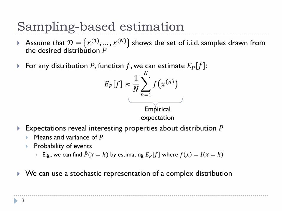
Assume that 𝒟 = 𝑥(1), … , 𝑥(𝑁) shows the set of i.i.d. samples drawn fromthe desired distribution 𝑃
For any distribution 𝑃, function 𝑓, we can estimate 𝐸𝑃 𝑓 :
𝐸𝑃 𝑓 ≈1
𝑁
𝑛=1
𝑁
𝑓 𝑥 𝑛
Expectations reveal interesting properties about distribution 𝑃 Means and variance of 𝑃 Probability of events
E.g., we can find 𝑃(𝑥 = 𝑘) by estimating 𝐸𝑃 𝑓 where 𝑓 𝑥 = 𝐼 𝑥 = 𝑘
We can use a stochastic representation of a complex distribution
Empirical
expectation
Bounds on error
4
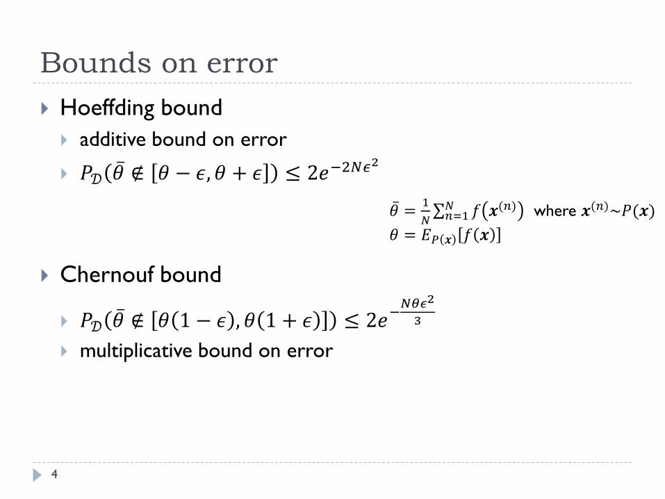
Hoeffding bound
additive bound on error
𝑃𝒟 𝜃 ∉ 𝜃 − 𝜖, 𝜃 + 𝜖 ≤ 2𝑒−2𝑁𝜖2
Chernouf bound
𝑃𝒟 𝜃 ∉ 𝜃 1 − 𝜖 , 𝜃 1 + 𝜖 ≤ 2𝑒−
𝑁𝜃𝜖2
3
multiplicative bound on error
𝜃 =1
𝑁 𝑛=1
𝑁 𝑓 𝒙(𝑛) where 𝒙(𝑛)~𝑃(𝒙)
𝜃 = 𝐸𝑃 𝒙 𝑓 𝒙
The mean and variance of the estimator
5
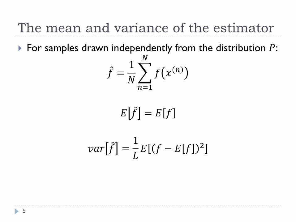
For samples drawn independently from the distribution 𝑃:
𝑓 =1
𝑁
𝑛=1
𝑁
𝑓 𝑥 𝑛
𝐸 𝑓 = 𝐸 𝑓
𝑣𝑎𝑟 𝑓 =1
𝐿𝐸 𝑓 − 𝐸 𝑓 2
Monte Carlo methods
6
Using a set of samples to find the answer of an inference query
expectations can be approximated using sample-based averages
Asymptotically exact and easy to apply to arbitrary
problems
Challenges:
Drawing samples from many distributions is not trivial
Are the gathered samples enough?
Are all samples useful, or equally useful?
Generating samples form a distribution
7
Assume that we have an algorithm that generates (pseudo-)
random numbers distributed uniformly over (0,1)
How do we generate a sample from these distributions.
First, we see simple cases:
Bernoulli
Multinomial
Other standard distributions
Transformation technique
8
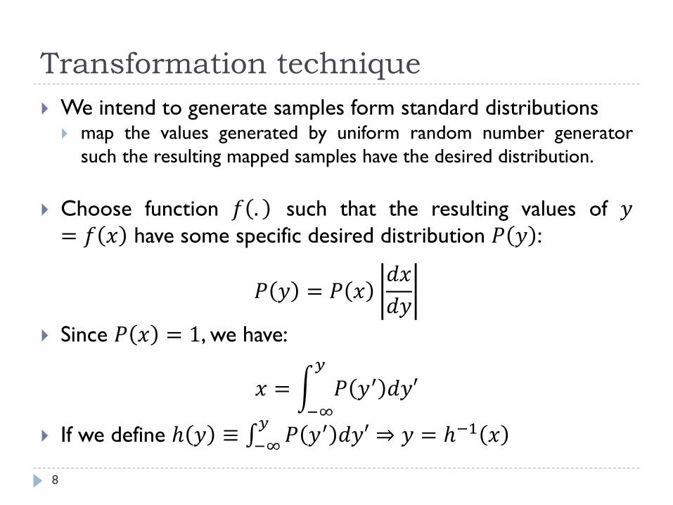
We intend to generate samples form standard distributions map the values generated by uniform random number generator
such the resulting mapped samples have the desired distribution.
Choose function 𝑓 . such that the resulting values of 𝑦= 𝑓 𝑥 have some specific desired distribution 𝑃 𝑦 :
𝑃 𝑦 = 𝑃 𝑥𝑑𝑥
𝑑𝑦
Since 𝑃 𝑥 = 1, we have:
𝑥 = −∞
𝑦
𝑃 𝑦′ 𝑑𝑦′
If we define ℎ 𝑦 ≡ −∞
𝑦𝑃 𝑦′ 𝑑𝑦′ ⇒ 𝑦 = ℎ−1 𝑥
Transformation technique
9
Cumulative CDF Sampling:
If 𝑥~𝑈(0,1), and ℎ(. ) is the CDF of 𝑃, then ℎ−1(𝑥) ~𝑃.
Since we need to calculate and then invert the indefinite integral of
𝑃, it will only be feasible for a limited number of simple distributions
Thus, we will see first rejection sampling and importance
sampling (in the next slides) that can be used as important
components in the more general sampling techniques.
Rejection sampling
10
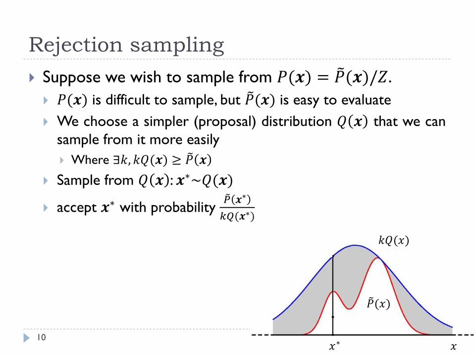
Suppose we wish to sample from 𝑃(𝒙) = 𝑃(𝒙)/𝑍.
𝑃(𝒙) is difficult to sample, but 𝑃(𝒙) is easy to evaluate
We choose a simpler (proposal) distribution 𝑄 𝒙 that we can
sample from it more easily
Where ∃𝑘, 𝑘𝑄(𝒙) ≥ 𝑃 𝒙
Sample from 𝑄 𝒙 : 𝒙∗~𝑄(𝒙)
accept 𝒙∗ with probability 𝑃 𝒙∗
𝑘𝑄(𝒙∗)
𝑘𝑄(𝑥)
𝑃(𝑥)
𝑥𝑥∗
Rejection sampling
11
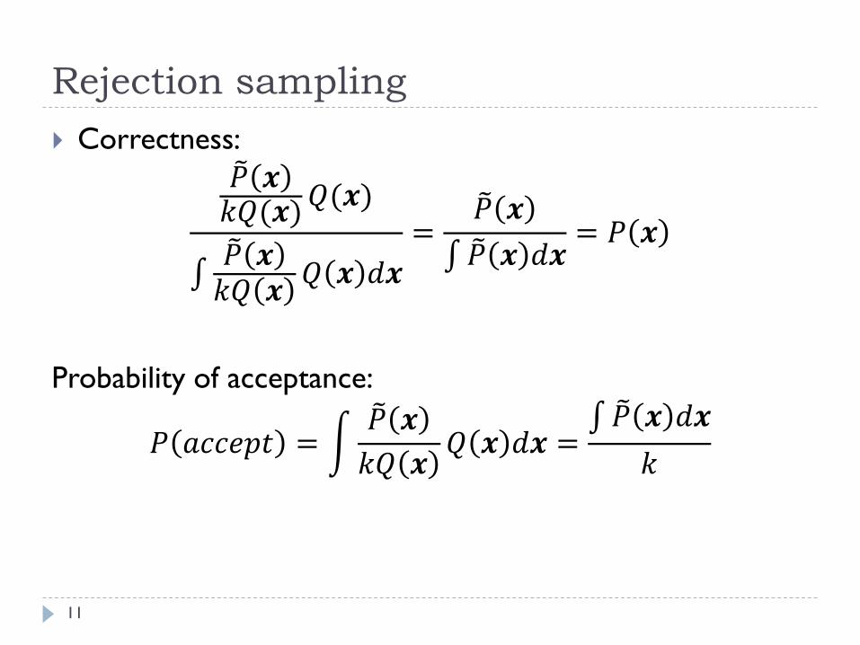
Correctness: 𝑃 𝒙
𝑘𝑄(𝒙)𝑄(𝒙)
𝑃 𝒙
𝑘𝑄 𝒙𝑄 𝒙 𝑑𝒙
= 𝑃 𝒙
𝑃 𝒙 𝑑𝒙= 𝑃 𝒙
Probability of acceptance:
𝑃 𝑎𝑐𝑐𝑒𝑝𝑡 = 𝑃 𝒙
𝑘𝑄 𝒙𝑄 𝒙 𝑑𝒙 =
𝑃 𝒙 𝑑𝒙
𝑘
Adaptive rejection sampling
12
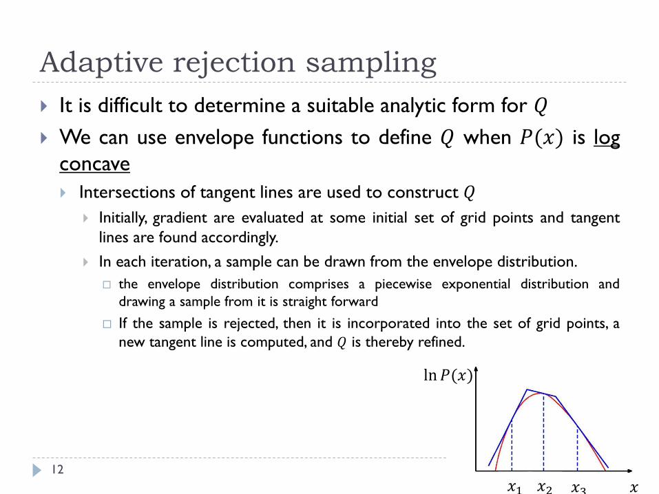
It is difficult to determine a suitable analytic form for 𝑄
We can use envelope functions to define 𝑄 when 𝑃(𝑥) is log
concave
Intersections of tangent lines are used to construct 𝑄
Initially, gradient are evaluated at some initial set of grid points and tangent
lines are found accordingly.
In each iteration, a sample can be drawn from the envelope distribution.
the envelope distribution comprises a piecewise exponential distribution and
drawing a sample from it is straight forward
If the sample is rejected, then it is incorporated into the set of grid points, a
new tangent line is computed, and 𝑄 is thereby refined.
ln 𝑃(𝑥)
𝑥1 𝑥2 𝑥3 𝑥
High dimensional rejection sampling
13
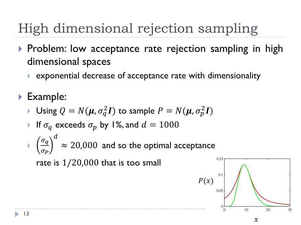
Problem: low acceptance rate rejection sampling in high
dimensional spaces
exponential decrease of acceptance rate with dimensionality
Example:
Using 𝑄 = 𝑁(𝝁, 𝜎𝑞2𝑰) to sample 𝑃 = 𝑁(𝝁, 𝜎𝑝
2𝑰)
If 𝜎𝑞 exceeds 𝜎𝑝 by 1%, and 𝑑 = 1000
𝜎𝑞
𝜎𝑃
𝑑
≈ 20,000 and so the optimal acceptance
rate is 1/20,000 that is too small
𝑃(𝑥)
𝑥
Importance sampling
14
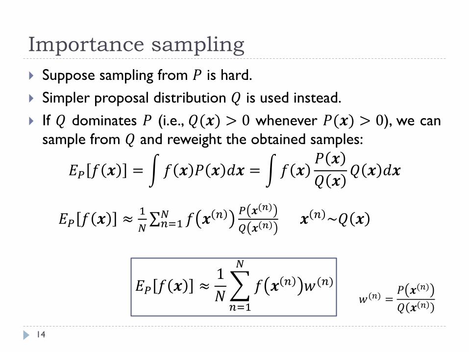
Suppose sampling from 𝑃 is hard.
Simpler proposal distribution 𝑄 is used instead.
If 𝑄 dominates 𝑃 (i.e., 𝑄(𝒙) > 0 whenever 𝑃(𝒙) > 0), we can
sample from 𝑄 and reweight the obtained samples:
𝐸𝑃 𝑓 𝒙 = 𝑓 𝒙 𝑃 𝒙 𝑑𝒙 = 𝑓 𝒙𝑃 𝒙
𝑄 𝒙𝑄 𝒙 𝑑𝒙
𝐸𝑃 𝑓 𝒙 ≈1
𝑁 𝑛=1
𝑁 𝑓 𝒙 𝑛 𝑃 𝒙(𝑛)
𝑄 𝒙 𝑛 𝒙 𝑛 ~𝑄 𝒙
𝐸𝑃 𝑓 𝒙 ≈1
𝑁
𝑛=1
𝑁
𝑓 𝒙 𝑛 𝑤(𝑛)
𝑤(𝑛) =𝑃 𝒙(𝑛)
𝑄 𝒙 𝑛
Normalized importance sampling
15
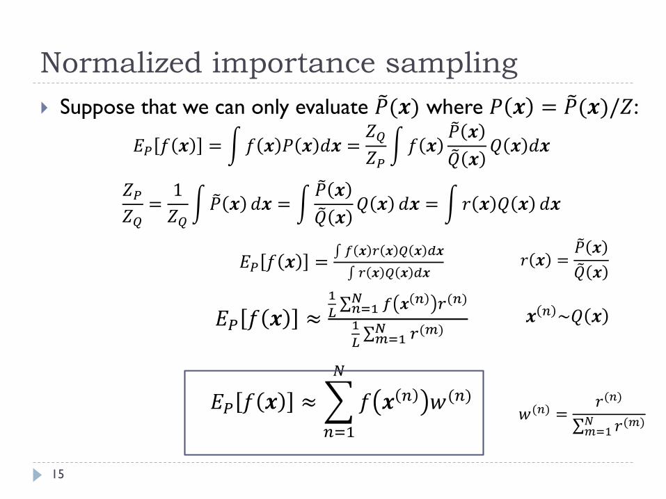
Suppose that we can only evaluate 𝑃(𝒙) where 𝑃 𝒙 = 𝑃(𝒙)/𝑍:
𝐸𝑃 𝑓 𝒙 = 𝑓 𝒙 𝑃 𝒙 𝑑𝒙 =𝑍𝑄
𝑍𝑃 𝑓 𝒙
𝑃 𝒙
𝑄 𝒙𝑄 𝒙 𝑑𝒙
𝑍𝑃
𝑍𝑄=
1
𝑍𝑄 𝑃 𝒙 𝑑𝒙 =
𝑃 𝒙
𝑄 𝒙𝑄 𝒙 𝑑𝒙 = 𝑟 𝒙 𝑄 𝒙 𝑑𝒙
𝐸𝑃 𝑓 𝒙 = 𝑓 𝒙 𝑟 𝒙 𝑄 𝒙 𝑑𝒙
𝑟 𝒙 𝑄 𝒙 𝑑𝒙
𝐸𝑃 𝑓 𝒙 ≈1
𝐿 𝑛=1
𝑁 𝑓 𝒙 𝑛 𝑟(𝑛)
1
𝐿 𝑚=1
𝑁 𝑟(𝑚)
𝐸𝑃 𝑓 𝒙 ≈
𝑛=1
𝑁
𝑓 𝒙 𝑛 𝑤(𝑛)
𝑟 𝒙 = 𝑃 𝒙
𝑄 𝒙
𝑤(𝑛) =𝑟(𝑛)
𝑚=1𝑁 𝑟(𝑚)
𝒙 𝑛 ~𝑄 𝒙
Importance sampling: problem
16
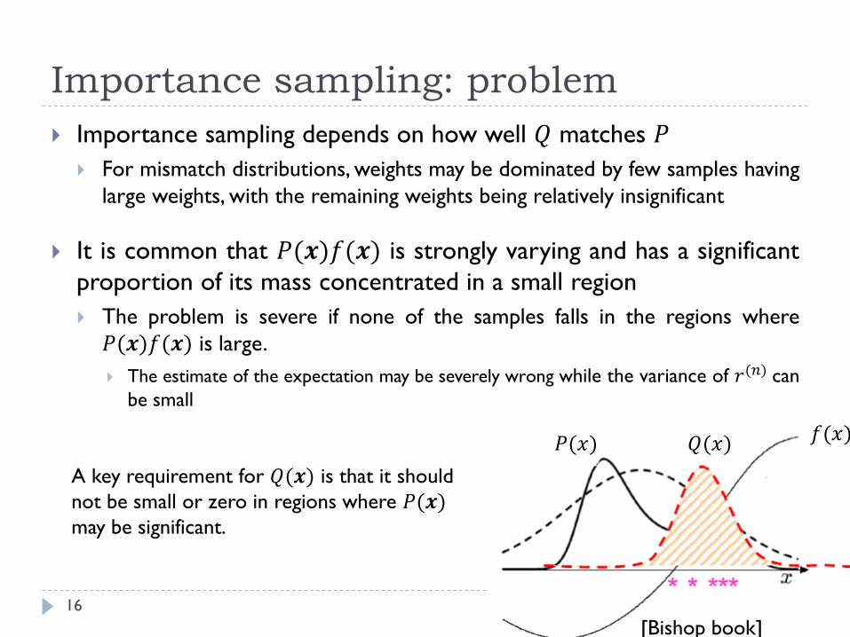
Importance sampling depends on how well 𝑄 matches 𝑃
For mismatch distributions, weights may be dominated by few samples having
large weights, with the remaining weights being relatively insignificant
It is common that 𝑃(𝒙)𝑓(𝒙) is strongly varying and has a significant
proportion of its mass concentrated in a small region
The problem is severe if none of the samples falls in the regions where
𝑃(𝒙)𝑓(𝒙) is large.
The estimate of the expectation may be severely wrong while the variance of 𝑟(𝑛) can
be small
𝑃(𝑥) 𝑄(𝑥) 𝑓(𝑥)
A key requirement for 𝑄(𝒙) is that it should
not be small or zero in regions where 𝑃(𝒙)may be significant.
[Bishop book]
Sampling Importance Resampling (SIR)
17
SIR sampling:
First, 𝐿 samples 𝒙(1), . . . , 𝒙(𝐿) are drawn from 𝑄(𝒙).
Then, weights 𝑤(1), . . . ,𝑤(𝑛) are found.
Finally, a second set of 𝐿 samples is drawn from the discrete distribution
𝒙(1), . . . , 𝒙(𝐿) with probabilities given by the weights 𝑤(1), . . . , 𝑤(𝑛) .
The resulting 𝐿 samples are only approximately
distributed according to 𝑃(𝒙) , but the distribution
becomes correct in the limit 𝐿 → ∞.
Sampling methods for graphical models
18
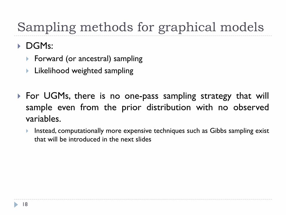
DGMs:
Forward (or ancestral) sampling
Likelihood weighted sampling
For UGMs, there is no one-pass sampling strategy that will
sample even from the prior distribution with no observed
variables.
Instead, computationally more expensive techniques such as Gibbs sampling exist
that will be introduced in the next slides
Sampling the joint distribution represented
by a BN
19
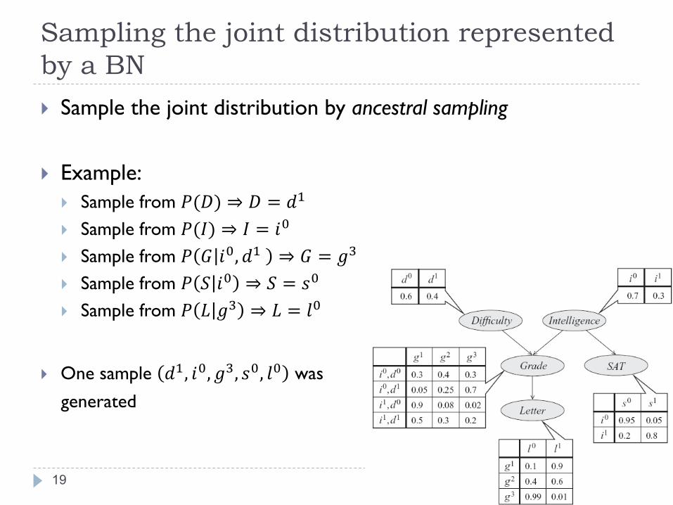
Sample the joint distribution by ancestral sampling
Example:
Sample from 𝑃(𝐷) ⇒ 𝐷 = 𝑑1
Sample from 𝑃(𝐼) ⇒ 𝐼 = 𝑖0
Sample from 𝑃 𝐺 𝑖0, 𝑑1 ⇒ 𝐺 = 𝑔3
Sample from 𝑃 𝑆 𝑖0 ⇒ 𝑆 = 𝑠0
Sample from 𝑃 𝐿 𝑔3 ⇒ 𝐿 = 𝑙0
One sample 𝑑1, 𝑖0, 𝑔3, 𝑠0, 𝑙0 was
generated
Forward sampling in a BN
20
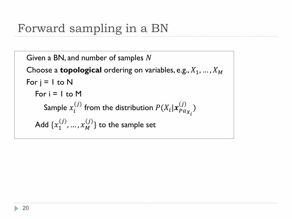
Given a BN, and number of samples 𝑁
Choose a topological ordering on variables, e.g., 𝑋1, … , 𝑋𝑀
For j = 1 to N
For i = 1 to M
Sample 𝑥𝑖(𝑗)
from the distribution 𝑃(𝑋𝑖|𝒙𝑃𝑎𝑋𝑖
(𝑗))
Add {𝑥1(𝑗)
, … , 𝑥𝑀(𝑗)
} to the sample set
Sampling for conditional probability query
21
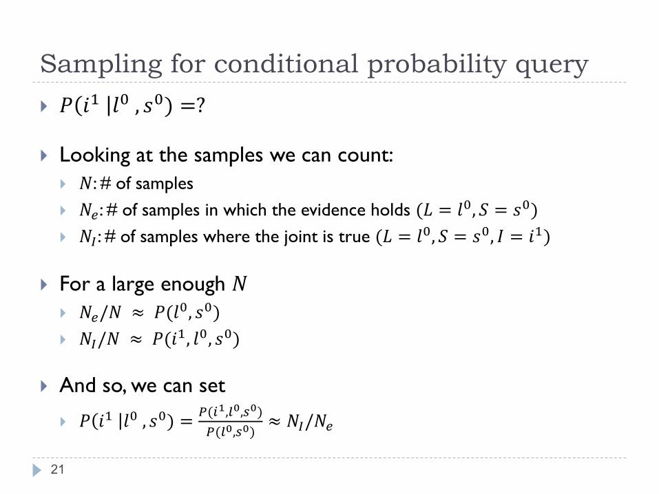
𝑃 𝑖1 𝑙0 , 𝑠0) =?
Looking at the samples we can count:
𝑁: # of samples
𝑁𝑒: # of samples in which the evidence holds (𝐿 = 𝑙0, 𝑆 = 𝑠0)
𝑁𝐼 : # of samples where the joint is true (𝐿 = 𝑙0, 𝑆 = 𝑠0, 𝐼 = 𝑖1)
For a large enough 𝑁 𝑁𝑒/𝑁 ≈ 𝑃(𝑙0, 𝑠0)
𝑁𝐼/𝑁 ≈ 𝑃(𝑖1, 𝑙0, 𝑠0)
And so, we can set
𝑃 𝑖1 𝑙0 , 𝑠0) =𝑃(𝑖1,𝑙0,𝑠0)
𝑃(𝑙0,𝑠0)≈ 𝑁𝐼/𝑁𝑒
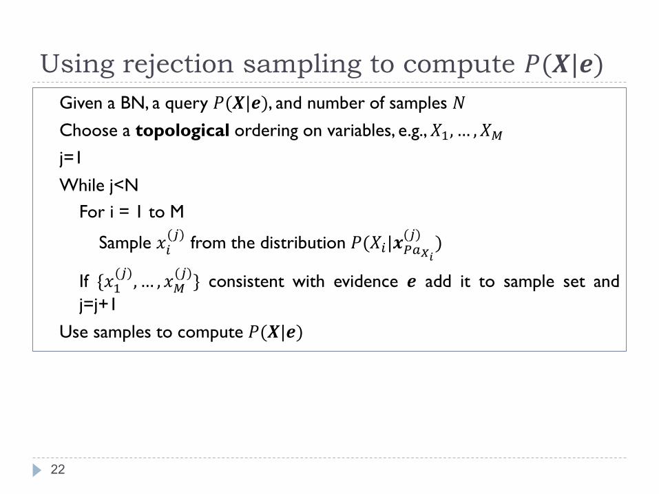
Using rejection sampling to compute 𝑃(𝑿|𝒆)
22
Given a BN, a query 𝑃(𝑿|𝒆), and number of samples 𝑁
Choose a topological ordering on variables, e.g., 𝑋1, … , 𝑋𝑀
j=1
While j<N
For i = 1 to M
Sample 𝑥𝑖(𝑗)
from the distribution 𝑃(𝑋𝑖|𝒙𝑃𝑎𝑋𝑖
(𝑗))
If {𝑥1(𝑗)
, … , 𝑥𝑀(𝑗)
} consistent with evidence 𝒆 add it to sample set and
j=j+1
Use samples to compute 𝑃(𝑿|𝒆)
Forward sampling: problem
23
Problem: When the evidence rarely happens, we would need
lots of samples, and most would be wasted
overall probability of accepting a sample rapidly decreases as the number
of observed variables increases and as the number of states that those
variables can take increases
This approach is very slow and rarely used in practice.
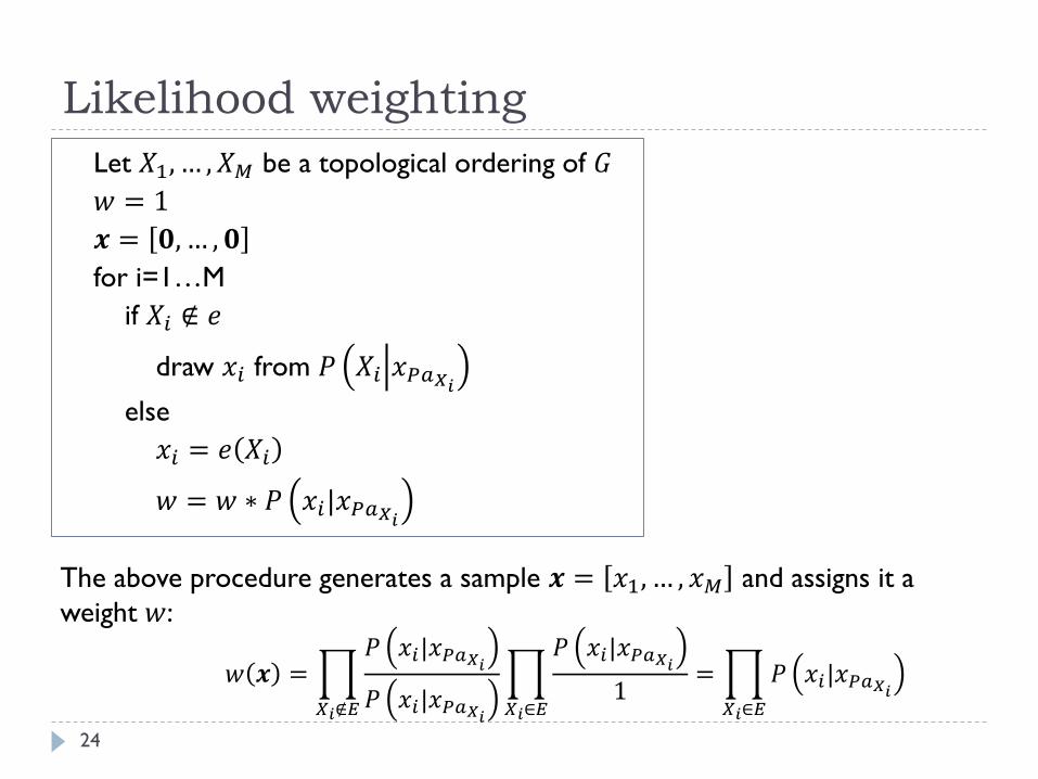
Likelihood weighting
24
Let 𝑋1, … , 𝑋𝑀 be a topological ordering of 𝐺
𝑤 = 1
𝒙 = 𝟎, … , 𝟎
for i=1…M
if 𝑋𝑖 ∉ 𝑒
draw 𝑥𝑖 from 𝑃 𝑋𝑖 𝑥𝑃𝑎𝑋𝑖
else
𝑥𝑖 = 𝑒 𝑋𝑖
𝑤 = 𝑤 ∗ 𝑃 𝑥𝑖|𝑥𝑃𝑎𝑋𝑖
𝑤 𝒙 =
𝑋𝑖∉𝐸
𝑃 𝑥𝑖|𝑥𝑃𝑎𝑋𝑖
𝑃 𝑥𝑖|𝑥𝑃𝑎𝑋𝑖
𝑋𝑖∈𝐸
𝑃 𝑥𝑖|𝑥𝑃𝑎𝑋𝑖
1=
𝑋𝑖∈𝐸
𝑃 𝑥𝑖|𝑥𝑃𝑎𝑋𝑖
The above procedure generates a sample 𝒙 = 𝑥1, … , 𝑥𝑀 and assigns it a
weight 𝑤:
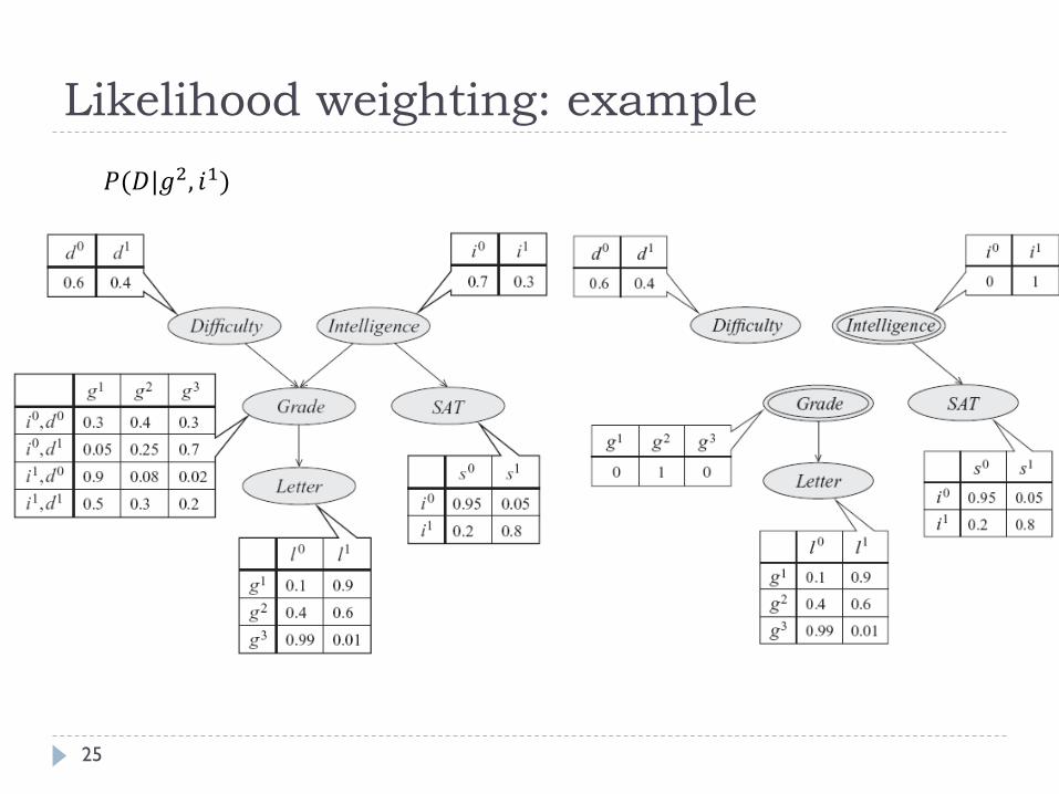
Likelihood weighting: example
25
𝑃(𝐷|𝑔2, 𝑖1)
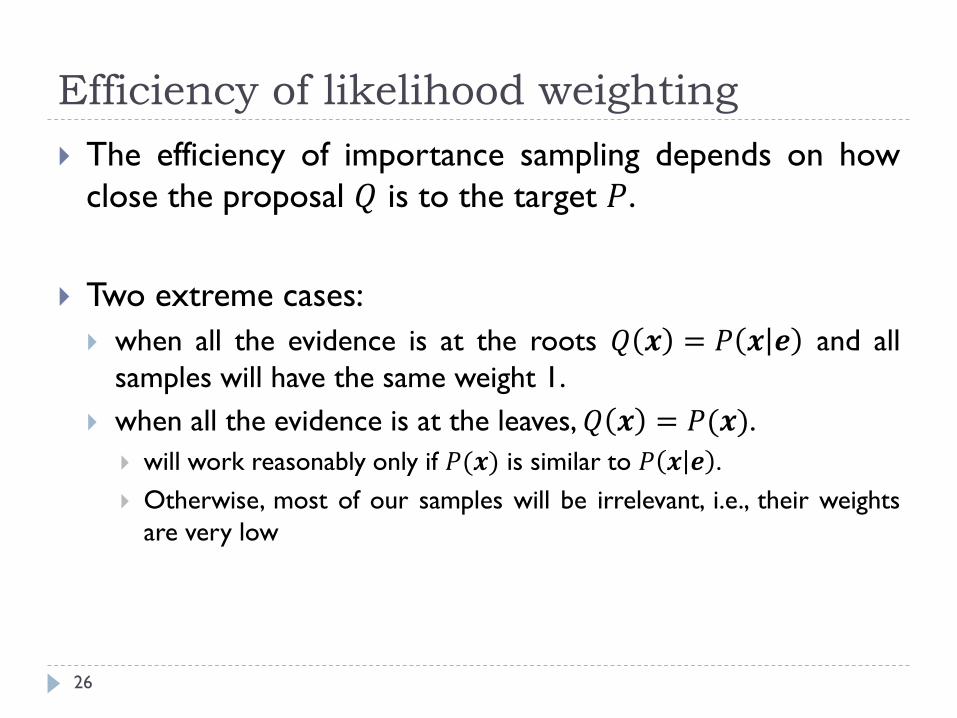
Efficiency of likelihood weighting
26
The efficiency of importance sampling depends on how
close the proposal 𝑄 is to the target 𝑃.
Two extreme cases:
when all the evidence is at the roots 𝑄 𝒙 = 𝑃 𝒙 𝒆 and all
samples will have the same weight 1.
when all the evidence is at the leaves, 𝑄 𝒙 = 𝑃(𝒙).
will work reasonably only if 𝑃(𝒙) is similar to 𝑃 𝒙 𝒆 .
Otherwise, most of our samples will be irrelevant, i.e., their weights
are very low
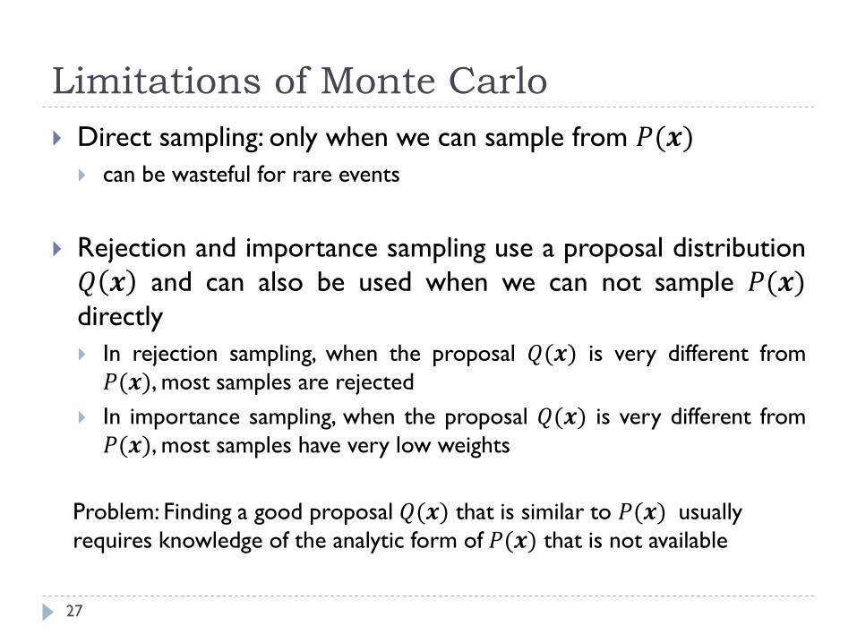
Limitations of Monte Carlo
27
Direct sampling: only when we can sample from 𝑃(𝒙) can be wasteful for rare events
Rejection and importance sampling use a proposal distribution
𝑄 𝒙 and can also be used when we can not sample 𝑃(𝒙)directly
In rejection sampling, when the proposal 𝑄(𝒙) is very different from
𝑃(𝒙), most samples are rejected
In importance sampling, when the proposal 𝑄(𝒙) is very different from
𝑃(𝒙), most samples have very low weights
Problem: Finding a good proposal 𝑄(𝒙) that is similar to 𝑃(𝒙) usually
requires knowledge of the analytic form of 𝑃(𝒙) that is not available
Markov chain Monte Carlo (MCMC)
28
Instead of using a fixed proposal 𝑄(𝒙), we can use an adaptive
proposal 𝑄(𝒙|𝒙(𝑡)) that depends on the last previous sample
𝒙(𝑡)
The proposal distribution is adapted as a function of the last accepted
sample
MCMC methods
Metropolis-Hasting
Gibbs
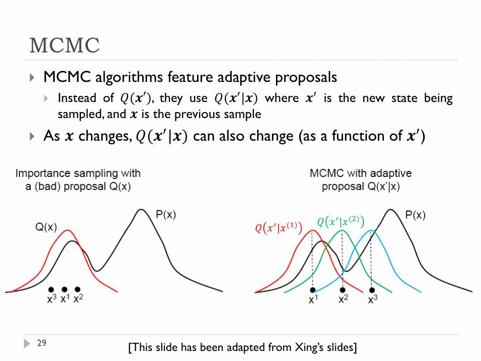
MCMC
29
MCMC algorithms feature adaptive proposals
Instead of 𝑄(𝒙′), they use 𝑄(𝒙′|𝒙) where 𝒙′ is the new state being
sampled, and 𝒙 is the previous sample
As 𝒙 changes, 𝑄(𝒙′|𝒙) can also change (as a function of 𝒙′)
𝑄 𝑥′|𝑥(1) 𝑄 𝑥′|𝑥(2)
[This slide has been adapted from Xing’s slides]
Metropolis-Hastings
30
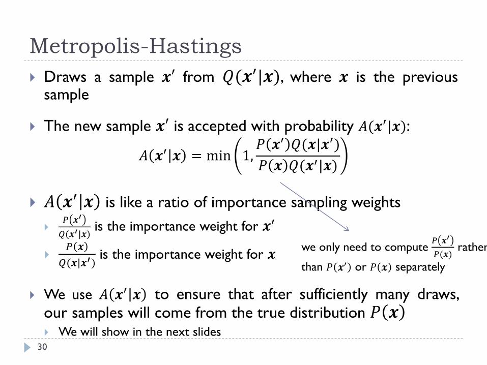
Draws a sample 𝒙′ from 𝑄(𝒙′|𝒙), where 𝒙 is the previoussample
The new sample 𝒙′ is accepted with probability 𝐴(𝒙′|𝒙):
𝐴 𝒙′ 𝒙 = min 1,𝑃 𝒙′ 𝑄(𝒙|𝒙′)
𝑃 𝒙 𝑄(𝒙′|𝒙)
𝐴 𝒙′ 𝒙 is like a ratio of importance sampling weights
𝑃 𝒙′
𝑄(𝒙′|𝒙)is the importance weight for 𝒙′
𝑃 𝒙
𝑄(𝒙|𝒙′)is the importance weight for 𝒙
We use 𝐴 𝒙′ 𝒙 to ensure that after sufficiently many draws,our samples will come from the true distribution 𝑃 𝒙 We will show in the next slides
we only need to compute 𝑃 𝒙′
𝑃(𝒙)rather
than 𝑃 𝒙′ or 𝑃 𝒙 separately
Metropolis-Hastings algorithm
31
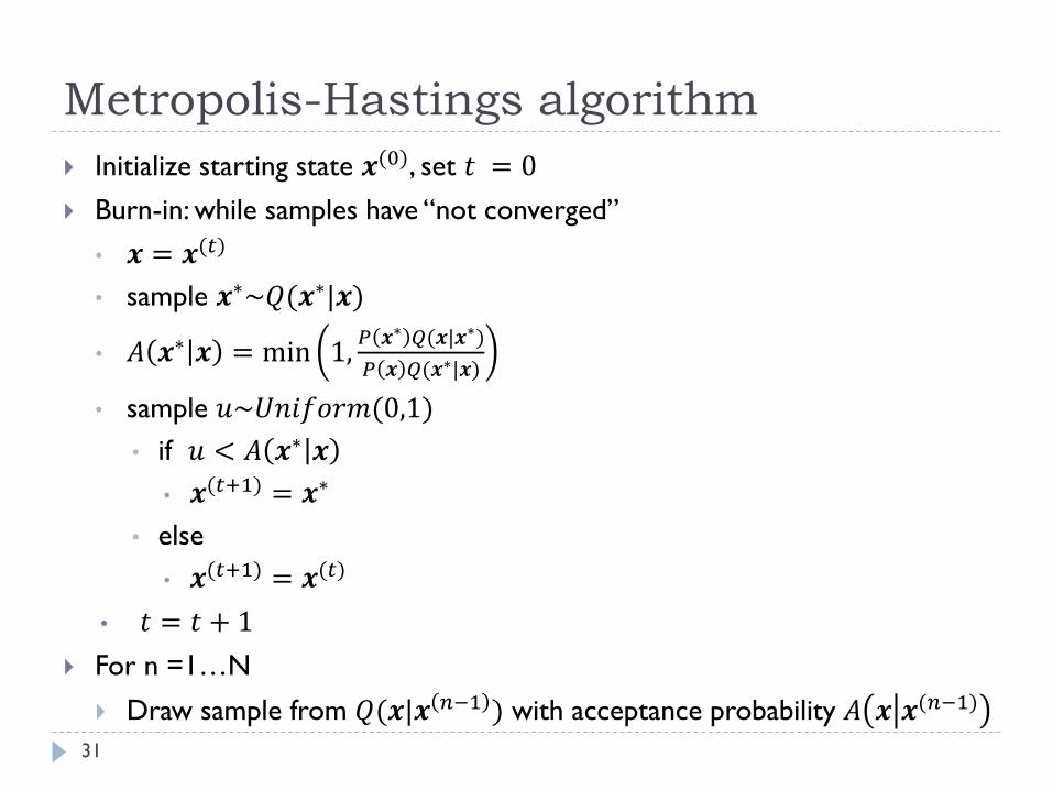
Initialize starting state 𝒙(0), set 𝑡 = 0
Burn-in: while samples have “not converged”
• 𝒙 = 𝒙(𝑡)
• sample 𝒙∗~𝑄(𝒙∗|𝒙)
• 𝐴 𝒙∗ 𝒙 = min 1,𝑃 𝒙∗ 𝑄(𝒙|𝒙∗)
𝑃 𝒙 𝑄(𝒙∗|𝒙)
• sample 𝑢~𝑈𝑛𝑖𝑓𝑜𝑟𝑚(0,1)
• if 𝑢 < 𝐴 𝒙∗ 𝒙
• 𝒙(𝑡+1) = 𝒙∗
• else
• 𝒙(𝑡+1) = 𝒙(𝑡)
• 𝑡 = 𝑡 + 1
For n =1…N
Draw sample from 𝑄(𝒙|𝒙 𝑛−1 ) with acceptance probability 𝐴 𝒙 𝒙(𝑛−1)
Metropolis-Hastings algorithm: Example
32
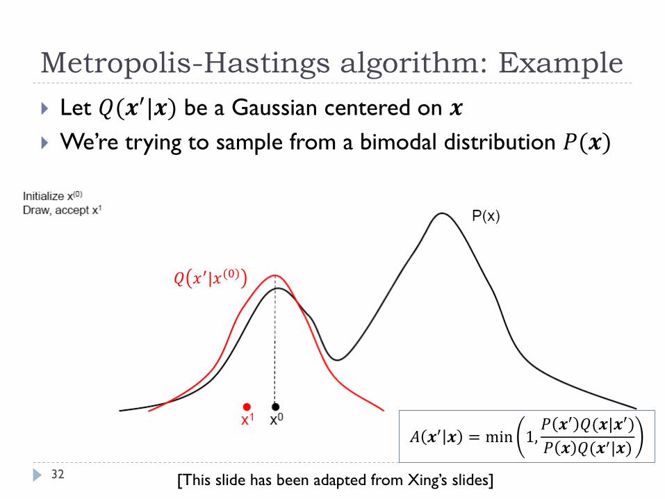
Let 𝑄(𝒙′|𝒙) be a Gaussian centered on 𝒙
We’re trying to sample from a bimodal distribution 𝑃(𝒙)
𝑄 𝑥′|𝑥(0)
[This slide has been adapted from Xing’s slides]
𝐴 𝒙′ 𝒙 = min 1,𝑃 𝒙′ 𝑄(𝒙|𝒙′)
𝑃 𝒙 𝑄(𝒙′|𝒙)
Metropolis-Hastings algorithm: Example
33
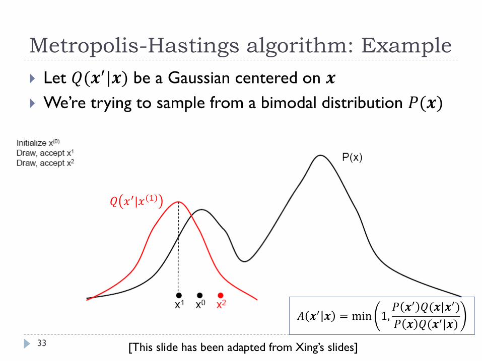
Let 𝑄(𝒙′|𝒙) be a Gaussian centered on 𝒙
We’re trying to sample from a bimodal distribution 𝑃(𝒙)
𝑄 𝑥′|𝑥(1)
[This slide has been adapted from Xing’s slides]
𝐴 𝒙′ 𝒙 = min 1,𝑃 𝒙′ 𝑄(𝒙|𝒙′)
𝑃 𝒙 𝑄(𝒙′|𝒙)
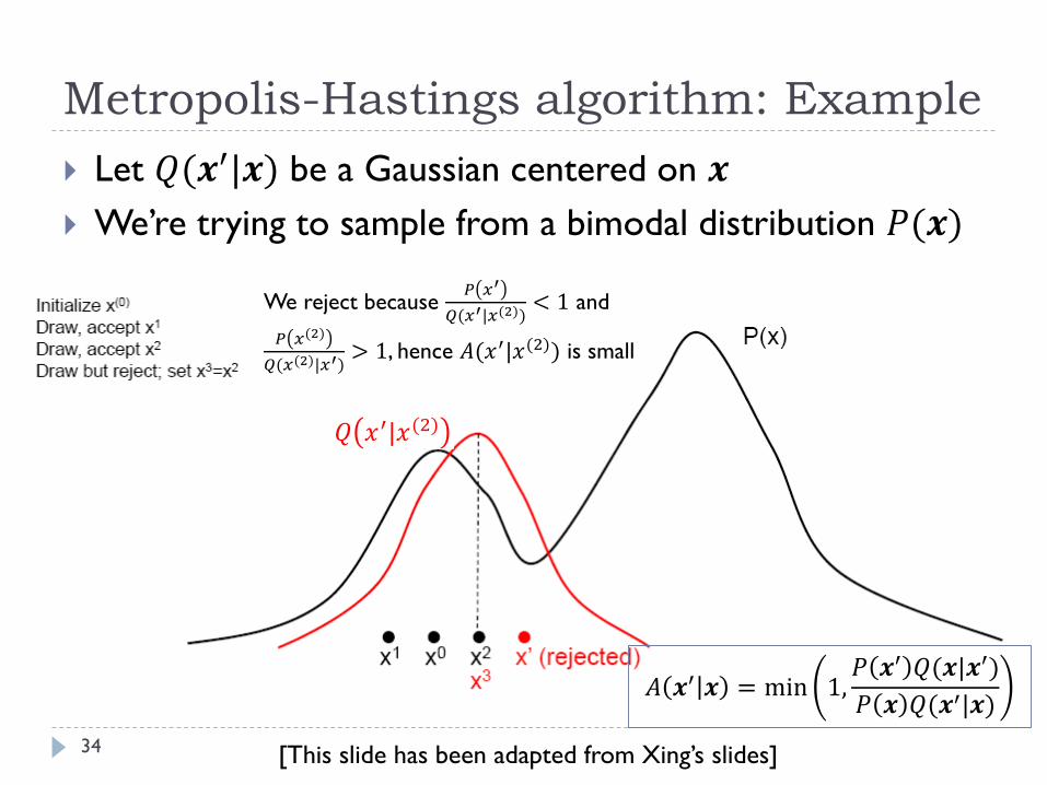
Metropolis-Hastings algorithm: Example
34
Let 𝑄(𝒙′|𝒙) be a Gaussian centered on 𝒙
We’re trying to sample from a bimodal distribution 𝑃(𝒙)
We reject because 𝑃 𝑥′
𝑄(𝑥′|𝑥(2))< 1 and
𝑃 𝑥(2)
𝑄(𝑥(2)|𝑥′)> 1, hence 𝐴(𝑥′|𝑥(2)) is small
𝑄 𝑥′|𝑥(2)
[This slide has been adapted from Xing’s slides]
𝐴 𝒙′ 𝒙 = min 1,𝑃 𝒙′ 𝑄(𝒙|𝒙′)
𝑃 𝒙 𝑄(𝒙′|𝒙)
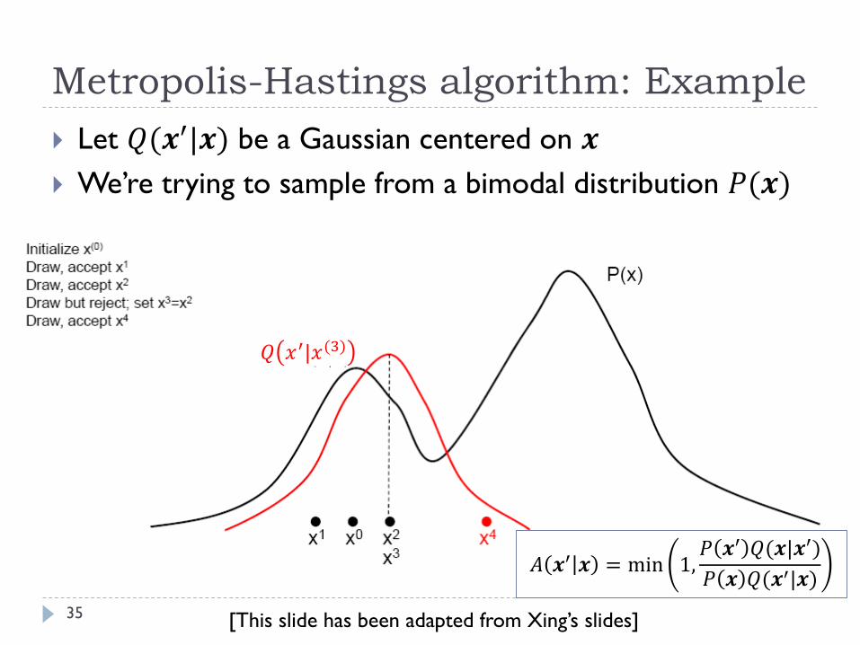
Metropolis-Hastings algorithm: Example
35
Let 𝑄(𝒙′|𝒙) be a Gaussian centered on 𝒙
We’re trying to sample from a bimodal distribution 𝑃(𝒙)
𝑄 𝑥′|𝑥(3)
[This slide has been adapted from Xing’s slides]
𝐴 𝒙′ 𝒙 = min 1,𝑃 𝒙′ 𝑄(𝒙|𝒙′)
𝑃 𝒙 𝑄(𝒙′|𝒙)
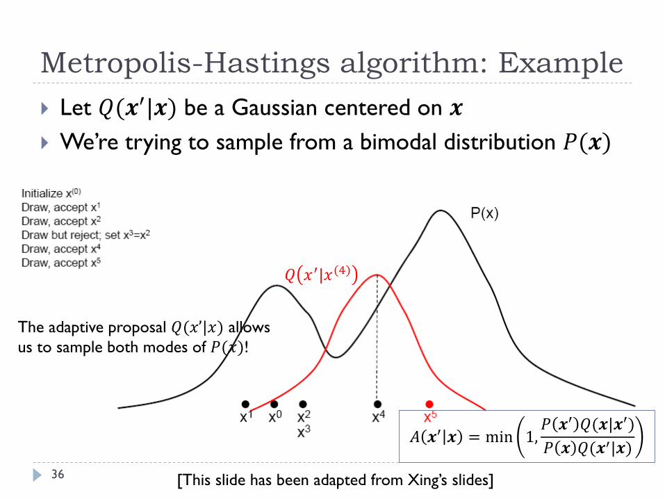
Metropolis-Hastings algorithm: Example
36
Let 𝑄(𝒙′|𝒙) be a Gaussian centered on 𝒙
We’re trying to sample from a bimodal distribution 𝑃(𝒙)
The adaptive proposal 𝑄(𝑥’|𝑥) allows
us to sample both modes of 𝑃(𝑥)!
𝑄 𝑥′|𝑥(4)
[This slide has been adapted from Xing’s slides]
𝐴 𝒙′ 𝒙 = min 1,𝑃 𝒙′ 𝑄(𝒙|𝒙′)
𝑃 𝒙 𝑄(𝒙′|𝒙)
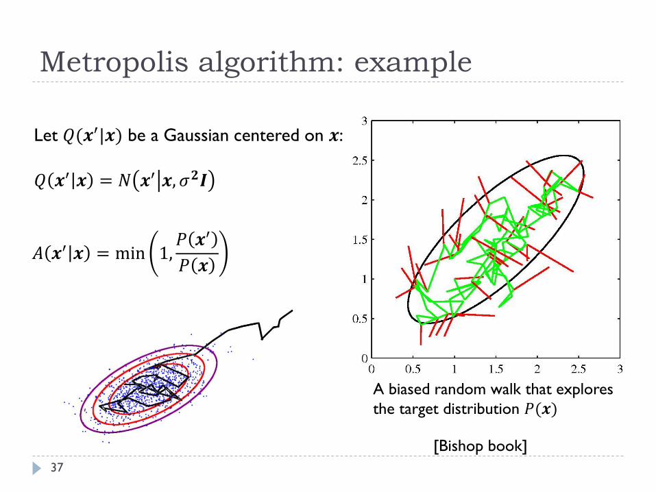
Metropolis algorithm: example
37
Let 𝑄(𝒙′|𝒙) be a Gaussian centered on 𝒙:
𝑄 𝒙′ 𝒙 = 𝑁 𝒙′ 𝒙, 𝜎𝟐𝑰
𝐴 𝒙′ 𝒙 = min 1,𝑃 𝒙′
𝑃 𝒙
A biased random walk that explores
the target distribution 𝑃(𝒙)
[Bishop book]
Metropolis algorithm: example
38
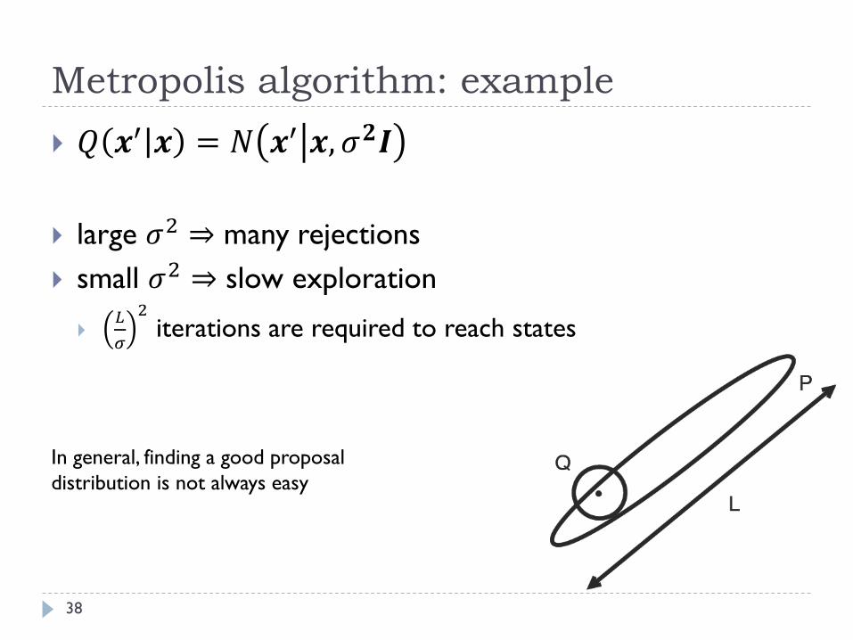
𝑄 𝒙′ 𝒙 = 𝑁 𝒙′ 𝒙, 𝜎𝟐𝑰
large 𝜎2 ⇒ many rejections
small 𝜎2 ⇒ slow exploration
𝐿
𝜎
2iterations are required to reach states
In general, finding a good proposal
distribution is not always easy
Proposal distribution
39
low-variance proposals:
high probability of acceptance
many iterations are required to explore 𝑃 𝒙
results in more correlated samples
high-variance proposals
low probability of acceptance
have the potential to explore much of 𝑃(𝒙)
Results in less correlated samples
How to use Markov chains for sampling
from 𝑃 𝒙 ?
40
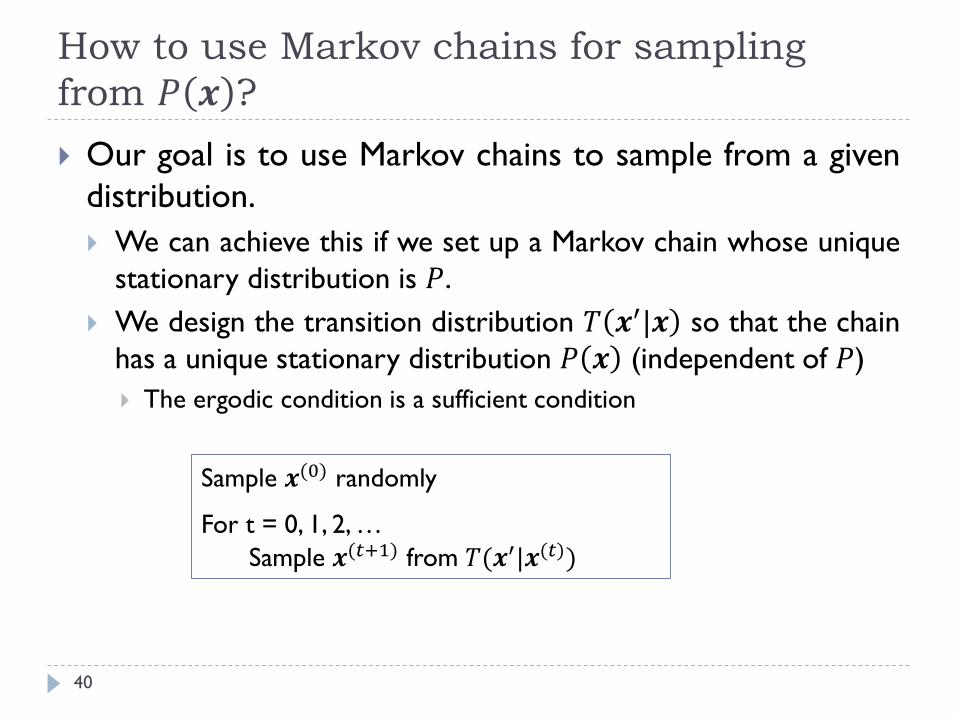
Our goal is to use Markov chains to sample from a given
distribution.
We can achieve this if we set up a Markov chain whose unique
stationary distribution is 𝑃.
We design the transition distribution 𝑇 𝒙′|𝒙 so that the chain
has a unique stationary distribution 𝑃 𝒙 (independent of 𝑃)
The ergodic condition is a sufficient condition
Sample 𝒙(0) randomly
For t = 0, 1, 2, …
Sample 𝒙(𝑡+1) from 𝑇(𝒙′|𝒙(𝑡))
Stationary distribution & detailed balance
41
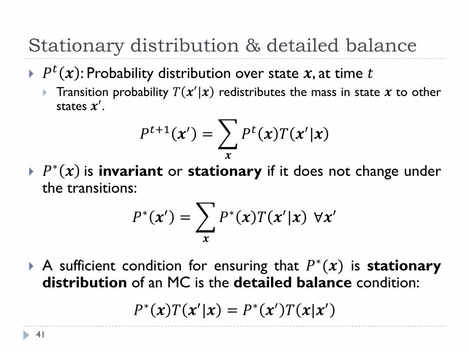
𝑃𝑡 𝒙 : Probability distribution over state 𝒙, at time 𝑡 Transition probability 𝑇 𝒙′|𝒙 redistributes the mass in state 𝒙 to other
states 𝒙′.
𝑃𝑡+1 𝒙′ =
𝒙
𝑃𝑡 𝒙 𝑇 𝒙′|𝒙
𝑃∗ 𝒙 is invariant or stationary if it does not change underthe transitions:
𝑃∗ 𝒙′ =
𝒙
𝑃∗ 𝒙 𝑇 𝒙′|𝒙 ∀𝒙′
A sufficient condition for ensuring that 𝑃∗(𝒙) is stationarydistribution of an MC is the detailed balance condition:
𝑃∗ 𝒙 𝑇 𝒙′|𝒙 = 𝑃∗ 𝒙′ 𝑇 𝒙|𝒙′
Why does Metropolis-Hastings work?
42
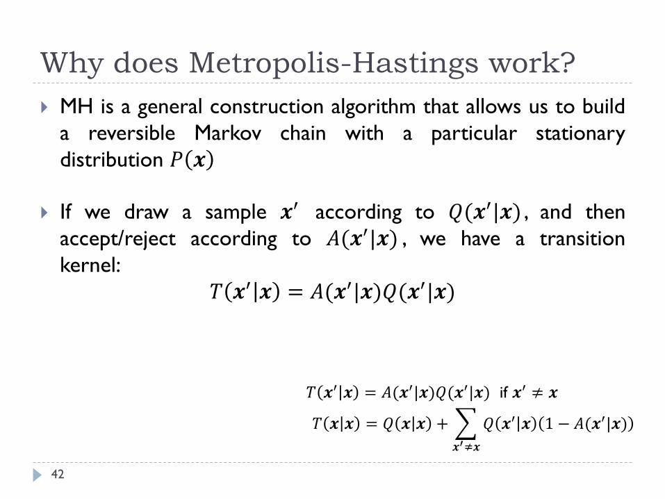
MH is a general construction algorithm that allows us to build
a reversible Markov chain with a particular stationary
distribution 𝑃 𝒙
If we draw a sample 𝒙′ according to 𝑄(𝒙′|𝒙) , and then
accept/reject according to 𝐴(𝒙′|𝒙) , we have a transition
kernel:
𝑇 𝒙′ 𝒙 = 𝐴(𝒙′|𝒙)𝑄(𝒙′|𝒙)
𝑇 𝒙′ 𝒙 = 𝐴(𝒙′|𝒙)𝑄(𝒙′|𝒙) if 𝒙′ ≠ 𝒙
𝑇 𝒙 𝒙 = 𝑄 𝒙 𝒙 +
𝒙′≠𝒙
𝑄 𝒙′ 𝒙 1 − 𝐴(𝒙′|𝒙)
MH satisfies detailed balance
43
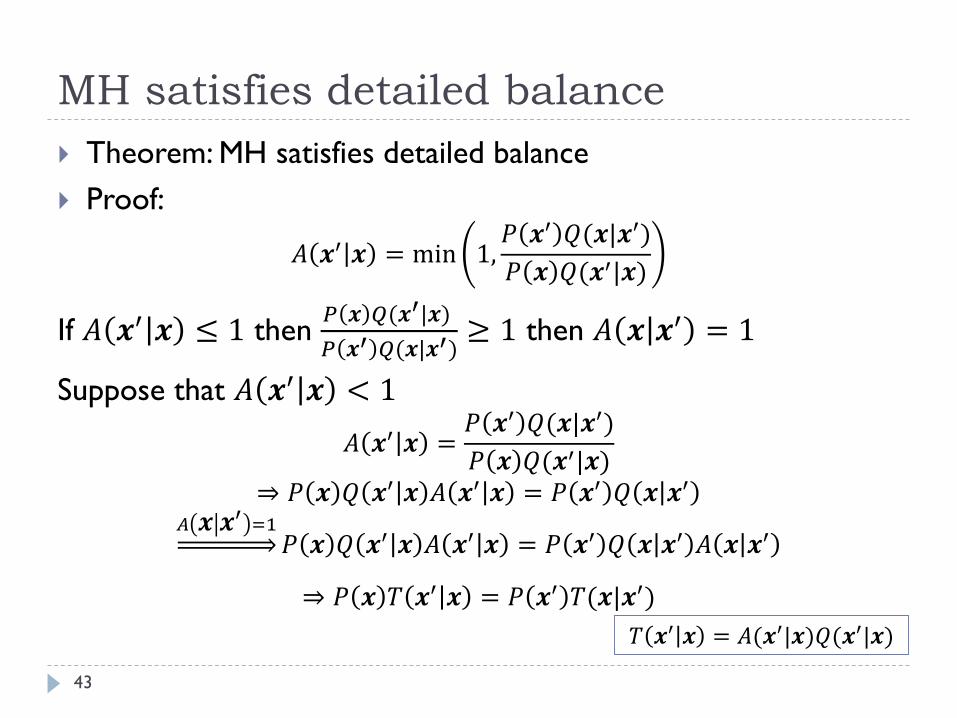
Theorem: MH satisfies detailed balance
Proof:
𝐴 𝒙′ 𝒙 = min 1,𝑃 𝒙′ 𝑄(𝒙|𝒙′)
𝑃 𝒙 𝑄(𝒙′|𝒙)
If 𝐴 𝒙′ 𝒙 ≤ 1 then𝑃 𝒙 𝑄(𝒙′|𝒙)
𝑃 𝒙′ 𝑄(𝒙|𝒙′)≥ 1 then 𝐴 𝒙 𝒙′ = 1
Suppose that 𝐴 𝒙′ 𝒙 < 1
𝐴 𝒙′ 𝒙 =𝑃 𝒙′ 𝑄(𝒙|𝒙′)
𝑃 𝒙 𝑄(𝒙′|𝒙)⇒ 𝑃 𝒙 𝑄 𝒙′ 𝒙 𝐴 𝒙′ 𝒙 = 𝑃 𝒙′ 𝑄 𝒙 𝒙′
𝐴 𝒙 𝒙′=1
𝑃 𝒙 𝑄 𝒙′ 𝒙 𝐴 𝒙′ 𝒙 = 𝑃 𝒙′ 𝑄 𝒙 𝒙′ 𝐴 𝒙 𝒙′
⇒ 𝑃 𝒙 𝑇 𝒙′ 𝒙 = 𝑃 𝒙′ 𝑇(𝒙|𝒙′)
𝑇 𝒙′ 𝒙 = 𝐴(𝒙′|𝒙)𝑄(𝒙′|𝒙)

MH properties
44
MH algorithm eventually converges to a stationary distribution
𝑃(𝒙) that is the true distribution
However, we have no guarantees as to when this will occur
the burn-in period is a way to ignore the un-converged part of the
Markov chain
but deciding when to halt burn-in is an art that needs experimentation.
𝑄 must be chosen to fulfill the technical requirements
Gibbs sampling algorithm
45
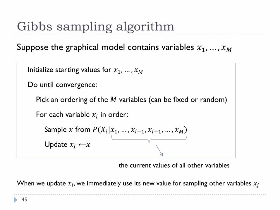
Initialize starting values for 𝑥1, … , 𝑥𝑀
Do until convergence:
Pick an ordering of the 𝑀 variables (can be fixed or random)
For each variable 𝑥𝑖 in order:
Sample 𝑥 from 𝑃(𝑋𝑖|𝑥1, … , 𝑥𝑖−1, 𝑥𝑖+1, … , 𝑥𝑀)
Update 𝑥𝑖 ←𝑥
When we update 𝑥𝑖, we immediately use its new value for sampling other variables 𝑥𝑗
Suppose the graphical model contains variables 𝑥1, … , 𝑥𝑀
the current values of all other variables
Gibbs sampling algorithm
46
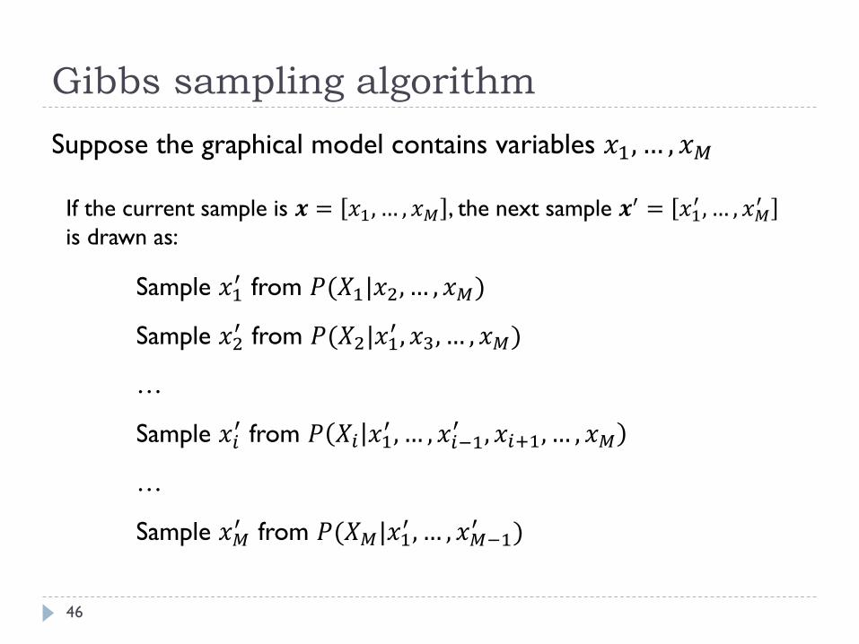
Sample 𝑥1′ from 𝑃(𝑋1|𝑥2, … , 𝑥𝑀)
Sample 𝑥2′ from 𝑃(𝑋2|𝑥1
′ , 𝑥3, … , 𝑥𝑀)
…
Sample 𝑥𝑖′ from 𝑃 𝑋𝑖 𝑥1
′ , … , 𝑥𝑖−1′ , 𝑥𝑖+1, … , 𝑥𝑀
…
Sample 𝑥𝑀′ from 𝑃(𝑋𝑀|𝑥1
′ , … , 𝑥𝑀−1′ )
Suppose the graphical model contains variables 𝑥1, … , 𝑥𝑀
If the current sample is 𝒙 = 𝑥1, … , 𝑥𝑀 , the next sample 𝒙′ = 𝑥1′ , … , 𝑥𝑀
′
is drawn as:
Gibbs Sampling
47
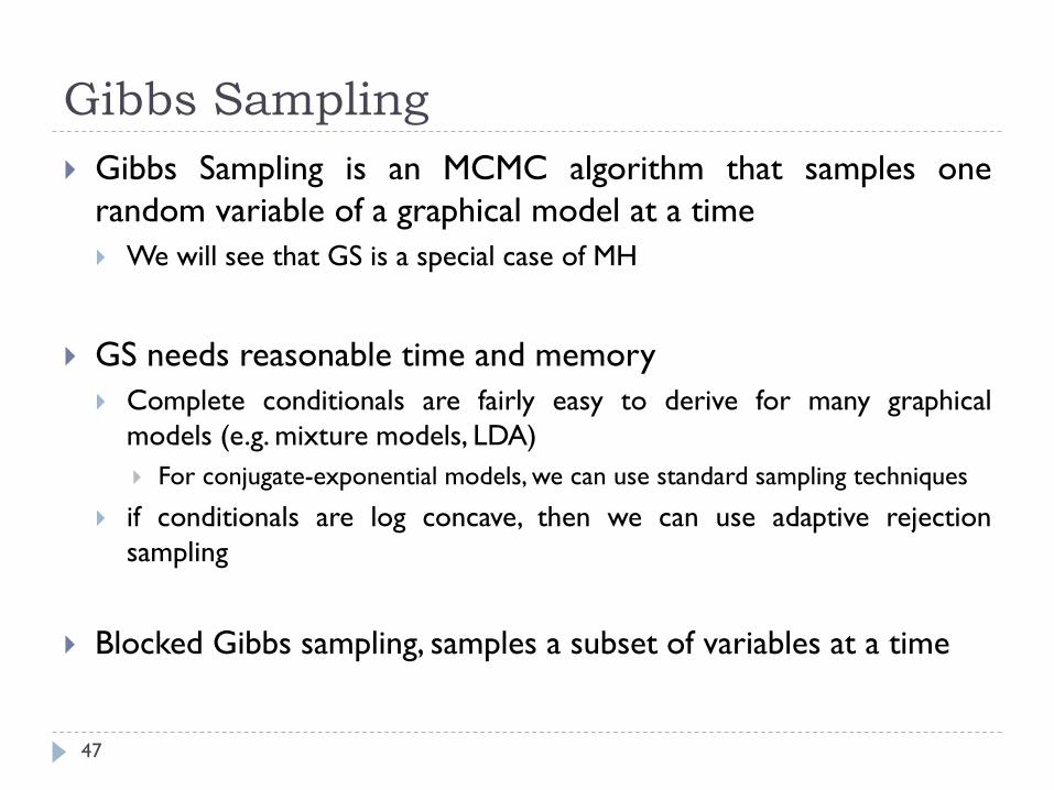
Gibbs Sampling is an MCMC algorithm that samples one
random variable of a graphical model at a time
We will see that GS is a special case of MH
GS needs reasonable time and memory
Complete conditionals are fairly easy to derive for many graphical
models (e.g. mixture models, LDA)
For conjugate-exponential models, we can use standard sampling techniques
if conditionals are log concave, then we can use adaptive rejection
sampling
Blocked Gibbs sampling, samples a subset of variables at a time
Gibbs sampling is a special case of MH
48
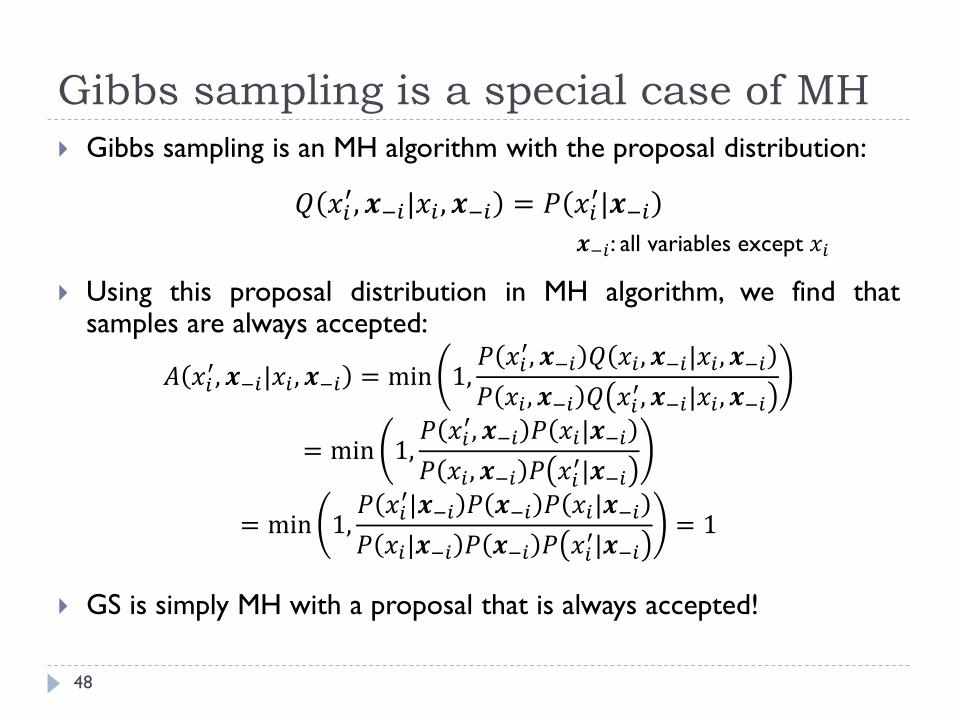
Gibbs sampling is an MH algorithm with the proposal distribution:
𝑄 𝑥𝑖′, 𝒙−𝑖|𝑥𝑖 , 𝒙−𝑖 = 𝑃 𝑥𝑖
′|𝒙−𝑖
Using this proposal distribution in MH algorithm, we find thatsamples are always accepted:
𝐴 𝑥𝑖′, 𝒙−𝑖|𝑥𝑖 , 𝒙−𝑖 = min 1,
𝑃 𝑥𝑖′, 𝒙−𝑖 𝑄 𝑥𝑖 , 𝒙−𝑖|𝑥𝑖 , 𝒙−𝑖
𝑃 𝑥𝑖 , 𝒙−𝑖 𝑄 𝑥𝑖′, 𝒙−𝑖|𝑥𝑖 , 𝒙−𝑖
= min 1,𝑃 𝑥𝑖
′, 𝒙−𝑖 𝑃 𝑥𝑖|𝒙−𝑖
𝑃 𝑥𝑖 , 𝒙−𝑖 𝑃 𝑥𝑖′|𝒙−𝑖
= min 1,𝑃 𝑥𝑖
′|𝒙−𝑖 𝑃 𝒙−𝑖 𝑃 𝑥𝑖|𝒙−𝑖
𝑃 𝑥𝑖|𝒙−𝑖 𝑃 𝒙−𝑖 𝑃 𝑥𝑖′|𝒙−𝑖
= 1
GS is simply MH with a proposal that is always accepted!
𝒙−𝑖: all variables except 𝑥𝑖
Gibbs sampling: example
49
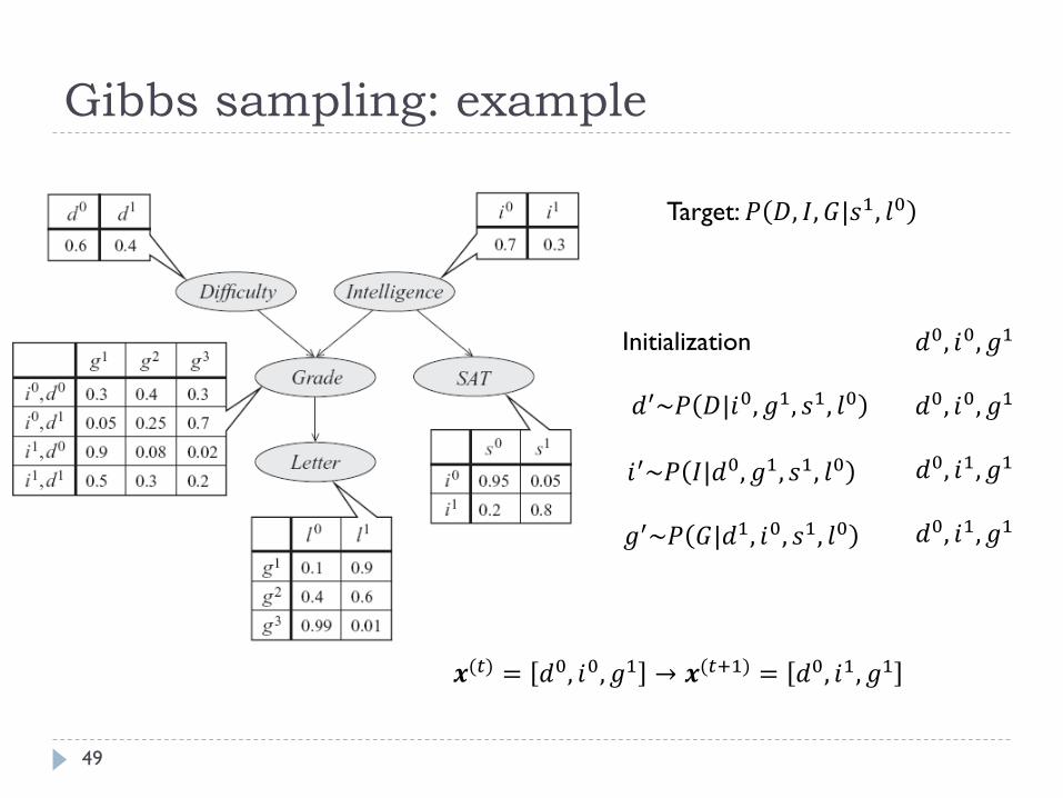
Target: 𝑃 𝐷, 𝐼, 𝐺|𝑠1, 𝑙0
𝑑0, 𝑖0, 𝑔1
𝑑0, 𝑖0, 𝑔1
𝑑0, 𝑖1, 𝑔1
𝑑0, 𝑖1, 𝑔1
Initialization
𝑑′~𝑃 𝐷|𝑖0, 𝑔1, 𝑠1, 𝑙0
𝑖′~𝑃 𝐼|𝑑0, 𝑔1, 𝑠1, 𝑙0
𝑔′~𝑃 𝐺|𝑑1, 𝑖0, 𝑠1, 𝑙0
𝒙(𝑡) = 𝑑0, 𝑖0, 𝑔1 → 𝒙(𝑡+1) = 𝑑0, 𝑖1, 𝑔1
Gibbs sampling:
complete conditional distributions
50
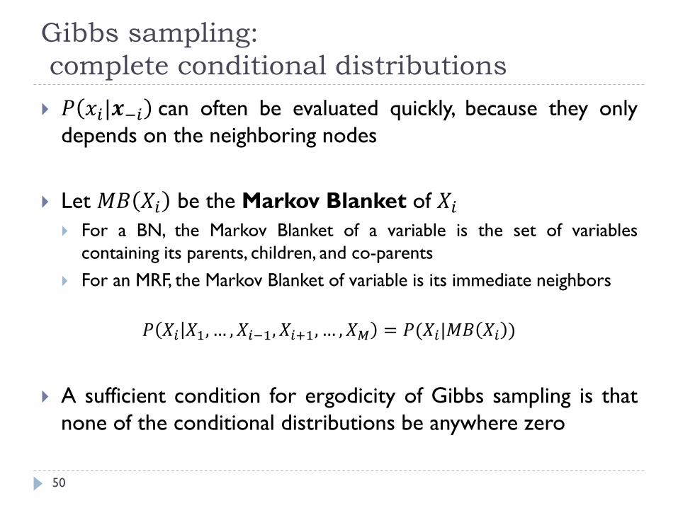
𝑃 𝑥𝑖|𝒙−𝑖 can often be evaluated quickly, because they only
depends on the neighboring nodes
Let 𝑀𝐵 𝑋𝑖 be the Markov Blanket of 𝑋𝑖
For a BN, the Markov Blanket of a variable is the set of variables
containing its parents, children, and co-parents
For an MRF, the Markov Blanket of variable is its immediate neighbors
𝑃 𝑋𝑖 𝑋1, … , 𝑋𝑖−1, 𝑋𝑖+1, … , 𝑋𝑀 = 𝑃(𝑋𝑖|𝑀𝐵 𝑋𝑖 )
A sufficient condition for ergodicity of Gibbs sampling is that
none of the conditional distributions be anywhere zero
Gibbs sampling implementation
51
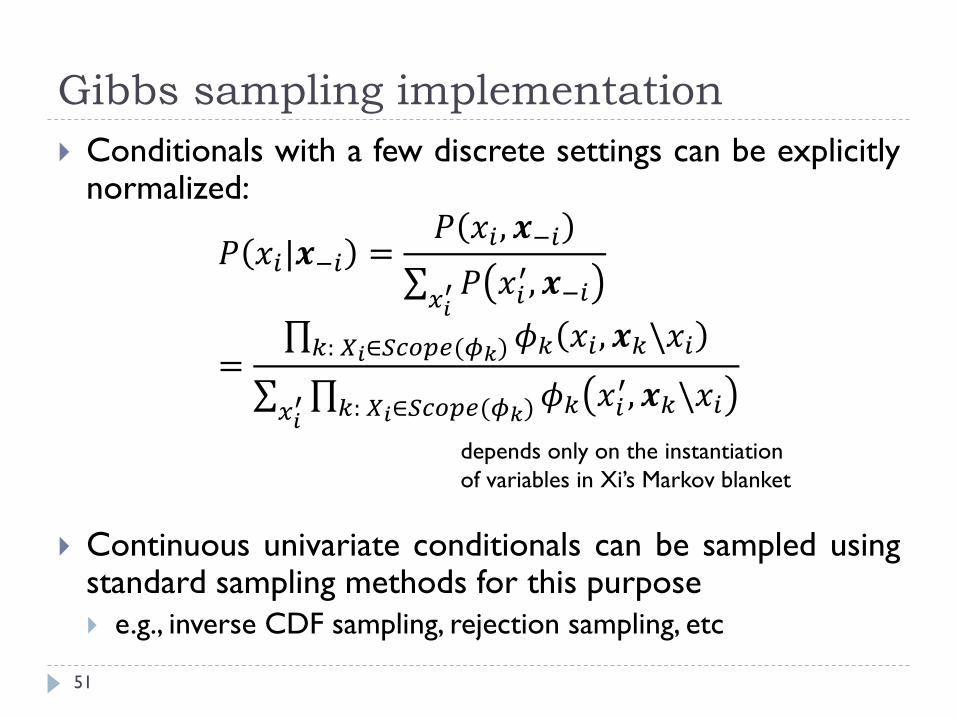
Conditionals with a few discrete settings can be explicitlynormalized:
𝑃 𝑥𝑖|𝒙−𝑖 =𝑃 𝑥𝑖 , 𝒙−𝑖
𝑥𝑖
′ 𝑃 𝑥𝑖′, 𝒙−𝑖
= 𝑘: 𝑋𝑖∈𝑆𝑐𝑜𝑝𝑒(𝜙𝑘) 𝜙𝑘 𝑥𝑖 , 𝒙𝑘\𝑥𝑖
𝑥𝑖
′ 𝑘: 𝑋𝑖∈𝑆𝑐𝑜𝑝𝑒(𝜙𝑘) 𝜙𝑘 𝑥𝑖′, 𝒙𝑘\𝑥𝑖
Continuous univariate conditionals can be sampled usingstandard sampling methods for this purpose
e.g., inverse CDF sampling, rejection sampling, etc
depends only on the instantiation
of variables in Xi’s Markov blanket
Gibbs sampling: summary
52
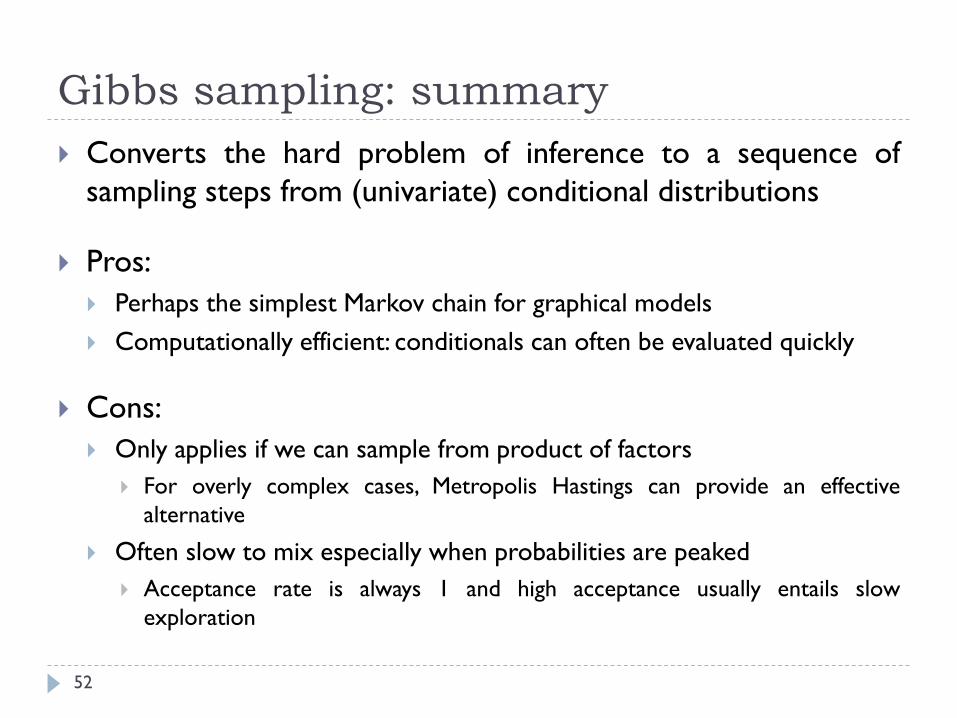
Converts the hard problem of inference to a sequence of
sampling steps from (univariate) conditional distributions
Pros:
Perhaps the simplest Markov chain for graphical models
Computationally efficient: conditionals can often be evaluated quickly
Cons:
Only applies if we can sample from product of factors
For overly complex cases, Metropolis Hastings can provide an effective
alternative
Often slow to mix especially when probabilities are peaked
Acceptance rate is always 1 and high acceptance usually entails slow
exploration
MH & MC: summary
53
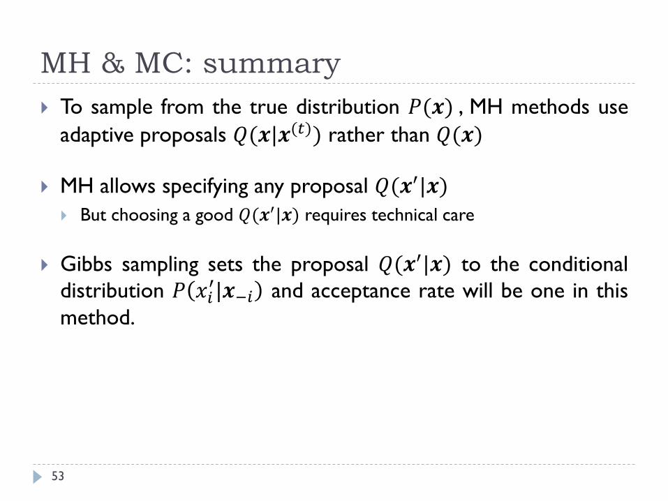
To sample from the true distribution 𝑃(𝒙) , MH methods use
adaptive proposals 𝑄(𝒙|𝒙(𝑡)) rather than 𝑄(𝒙)
MH allows specifying any proposal 𝑄(𝒙′|𝒙) But choosing a good 𝑄(𝒙′|𝒙) requires technical care
Gibbs sampling sets the proposal 𝑄(𝒙′|𝒙) to the conditional
distribution 𝑃 𝑥𝑖′|𝒙−𝑖 and acceptance rate will be one in this
method.
Practical aspects of MCMC
54
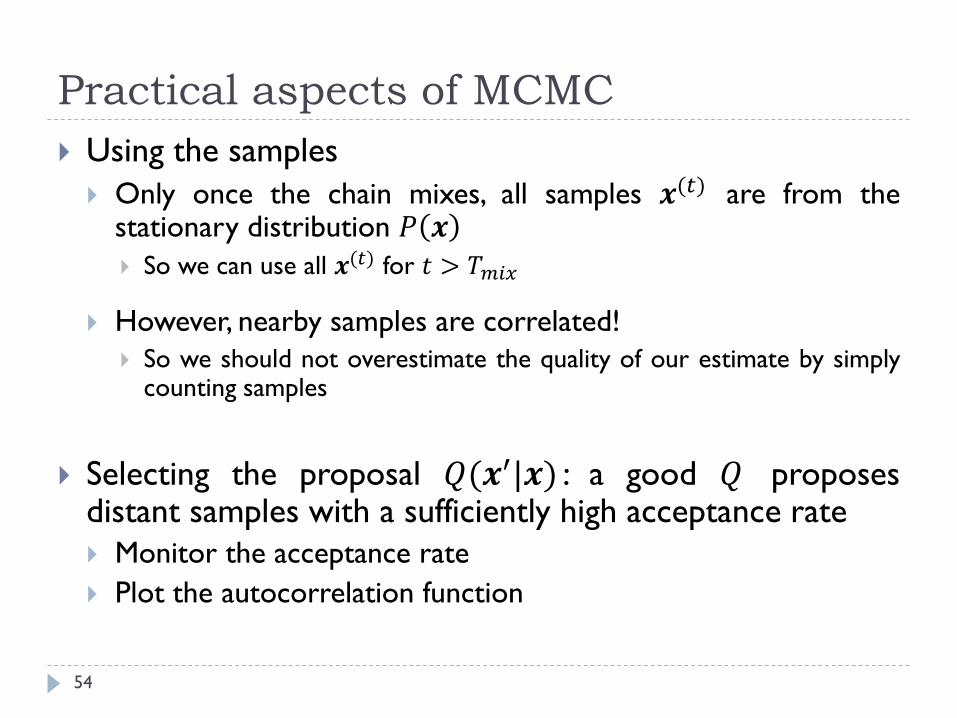
Using the samples
Only once the chain mixes, all samples 𝒙(𝑡) are from thestationary distribution 𝑃 𝒙 So we can use all 𝒙(𝑡) for 𝑡 > 𝑇𝑚𝑖𝑥
However, nearby samples are correlated!
So we should not overestimate the quality of our estimate by simplycounting samples
Selecting the proposal 𝑄(𝒙′|𝒙) : a good 𝑄 proposesdistant samples with a sufficiently high acceptance rate
Monitor the acceptance rate
Plot the autocorrelation function
Stop burn-in
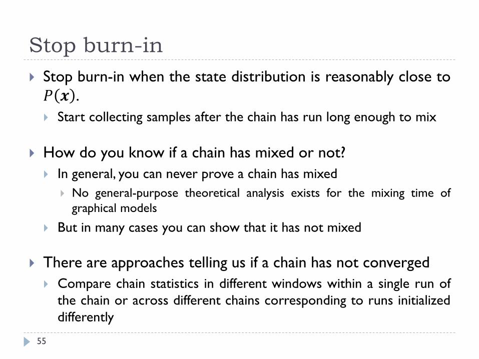
55
Stop burn-in when the state distribution is reasonably close to
𝑃 𝒙 .
Start collecting samples after the chain has run long enough to mix
How do you know if a chain has mixed or not?
In general, you can never prove a chain has mixed
No general-purpose theoretical analysis exists for the mixing time of
graphical models
But in many cases you can show that it has not mixed
There are approaches telling us if a chain has not converged
Compare chain statistics in different windows within a single run of
the chain or across different chains corresponding to runs initialized
differently
Poor mixing
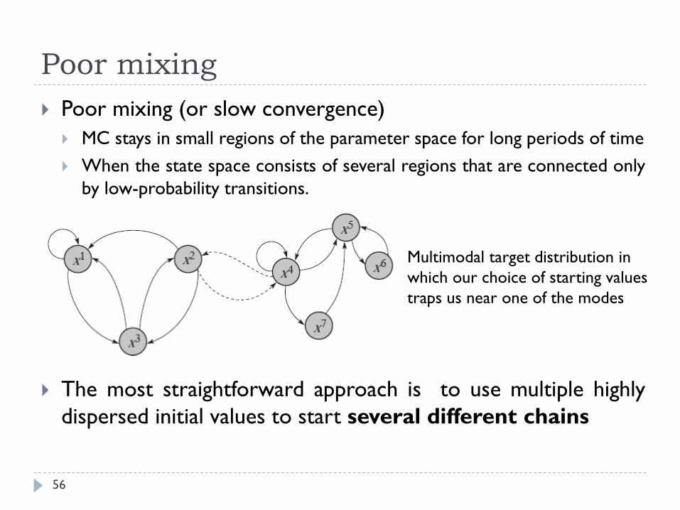
56
Poor mixing (or slow convergence)
MC stays in small regions of the parameter space for long periods of time
When the state space consists of several regions that are connected only
by low-probability transitions.
The most straightforward approach is to use multiple highly
dispersed initial values to start several different chains
Multimodal target distribution in
which our choice of starting values
traps us near one of the modes
Mixing?
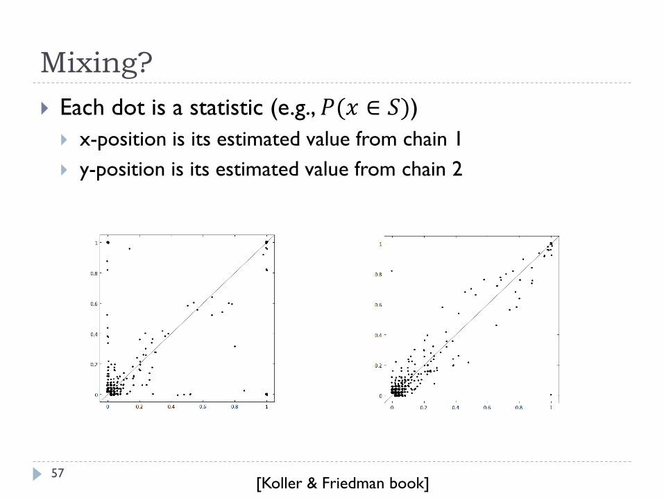
57
Each dot is a statistic (e.g., 𝑃(𝑥 ∈ 𝑆))
x-position is its estimated value from chain 1
y-position is its estimated value from chain 2
[Koller & Friedman book]
Autocorrelation coefficient
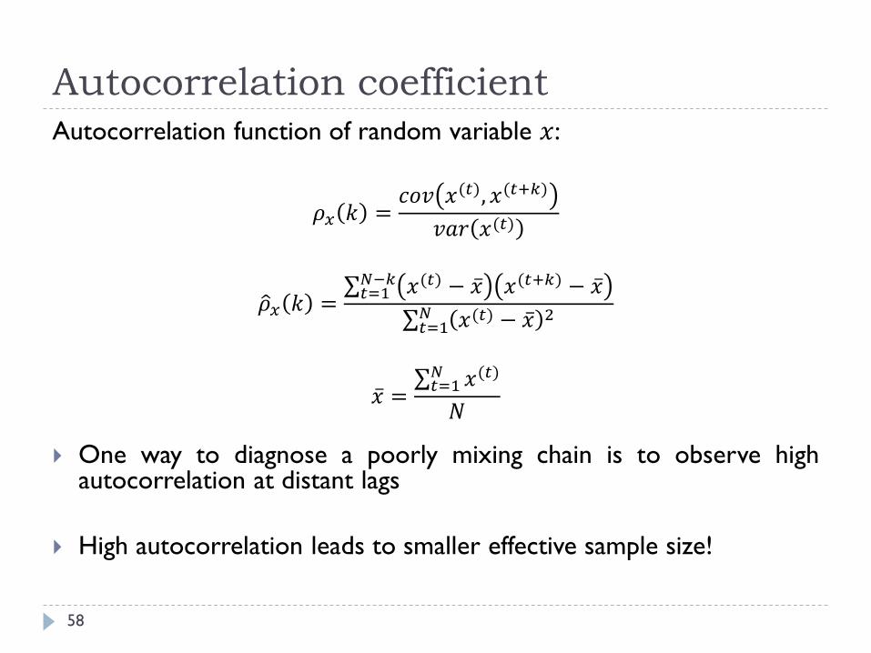
58
Autocorrelation function of random variable 𝑥:
𝜌𝑥 𝑘 =𝑐𝑜𝑣 𝑥(𝑡), 𝑥(𝑡+𝑘)
𝑣𝑎𝑟 𝑥(𝑡)
𝜌𝑥 𝑘 = 𝑡=1
𝑁−𝑘 𝑥(𝑡) − 𝑥 𝑥(𝑡+𝑘) − 𝑥
𝑡=1𝑁 𝑥(𝑡) − 𝑥 2
𝑥 = 𝑡=1
𝑁 𝑥(𝑡)
𝑁
One way to diagnose a poorly mixing chain is to observe highautocorrelation at distant lags
High autocorrelation leads to smaller effective sample size!
Thinning
59
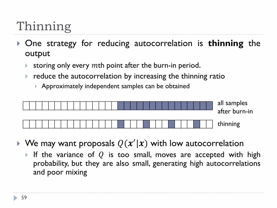
One strategy for reducing autocorrelation is thinning theoutput
storing only every 𝑚th point after the burn-in period.
reduce the autocorrelation by increasing the thinning ratio
Approximately independent samples can be obtained
We may want proposals 𝑄(𝒙′|𝒙) with low autocorrelation
If the variance of 𝑄 is too small, moves are accepted with highprobability, but they are also small, generating high autocorrelationsand poor mixing
thinning
all samples
after burn-in
Thinning or not?
60
All of the samples produces a provably better estimator than
using just remained after thinning
Thinning is useful primarily in settings where there is a
significant cost associated with using each sample (for example,
the evaluation of f is costly)
so that we might want to reduce the overall number of particles used.
One long chain or many smaller chains
61
If long burn-in periods are required, or if the chains have very
high autocorrelations:
using a large number of smaller chains may result in each not being
long enough to be of any value.
A good strategy: run a small number of chains in parallel for a
reasonably long time
using their behavior to evaluate mixing.

MCMC implementation details
62
Tunable parameters or design choices in MCMC:
the proposal distribution
the metrics for evaluating mixing
the number of chains to run
techniques for determining the thinning ratio
MCMC sampling: summary
63
Theoretical guarantees for convergence to exact values
However, it can be quite slow to converge We may need ridiculously many samples
only useful if the chain we are using mixes reasonably quickly
And it is difficult to tell whether it has been converged
Many options that need to be specified The application of Markov chains is more of an art than a science
Unlike forward sampling methods, MCMC methods: do not degrade when the probability of the evidence is low, or when the
posterior is very different from the prior.
apply to undirected models as well as to directed models.
Resources
64
D. Koller and N. Friedman, “Probabilistic Graphical Models:
Principles and Techniques”, Chapter 12.
C.M. Bishop, “Pattern Recognition and Machine Learning”,
Springer, Chapter 11.
Theoretical foundation of MH
65
Why are the samples generated by MH method will eventually
come from 𝑃(𝒙)?
Why does the MH algorithm have a “burn-in” period?
Markov chains
66
A Markov chain is a sequence of random variables 𝒙(1), … , 𝒙(𝑡)
with the Markov property
𝑃 𝒙(𝑡)|𝒙(1), … , 𝒙(𝑡−1) = 𝑃 𝒙(𝑡)|𝒙(𝑡−1)
We focus on homogeneous Markov chains, in which
𝑃 𝒙(𝑡)|𝒙(𝑡−1) is fixed with time
Let 𝒙 be the previous state and 𝒙′ be the next state, we call
𝑃 𝒙(𝑡)|𝒙(𝑡−1) as 𝑇 𝒙′|𝒙
Thus, at each time point, 𝒙(𝑡) is a state showing the
configuration of all the variables in the model
Markov chains: invariant or stationary dist.
67
𝜋𝑡 𝒙 : Probability distribution over state 𝒙, at time 𝑡 Transition probability 𝑇 𝒙′|𝒙 redistributes the mass in state 𝒙 to other
states 𝒙′.
𝜋𝑡 𝒙′ =
𝒙
𝜋𝑡 𝒙 𝑇 𝒙′|𝒙
𝜋 𝒙 is invariant or stationary if it does not change under
the transitions:
𝜋 𝒙′ =
𝒙
𝜋 𝒙 𝑇 𝒙′|𝒙 ∀𝒙′
𝑇 𝒙′|𝒙 = 𝑃 𝒙(𝑡) = 𝒙′|𝒙 𝑡−1 = 𝒙
Invariant distributions are of great importance in MCMC methods.
More specific than stationary distribution
68
There is also no guarantees that the stationary distribution is
unique.
In some chains, the stationary distribution reached depends on
our starting distribution 𝜋0(𝒙).
We want to restrict our attention to MCs that have a unique
stationary distribution, which is reached from any starting
distribution 𝜋0(𝒙).
There are various conditions that suffice to guarantee this
property.
The most commonly used condition is ergodicity.
Equilibrium distribution
69
Stationary distribution 𝜋 of transition probabilities 𝑇 is called
the equilibrium distribution when lim𝑡→∞
𝜋𝑡 = 𝜋 independent
of the initial distribution 𝜋0
Ergodicity implies you can reach the stationary distribution 𝜋(𝒙), no
matter the initial distribution 𝜋0(𝒙)
Clearly, an ergodic Markov chain can have only one equilibrium
distribution.
Ergodic Markov chain
70
A homogeneous Markov chain will be ergodic, subject only to
the following conditions:
Irreducible: an MC is irreducible if we can get from any state 𝒙 to any
other state 𝒙′ with probability > 0 in a finite number of steps
Aperiodic: an MC is aperiodic if you can return to any state 𝒙 at any
time
Periodic MCs have states that need ≥2 time steps to return to (cycles)
Ergodic: an MC is ergodic if it is irreducible and aperiodic
An ergodic MC converges to a unique stationary distribution regardless
of the start state
Finite state space MC
71
A Markov chain is ergodic or regular if there exists 𝑘such that, for every 𝒙, 𝒙′, the probability of getting from 𝒙to 𝒙′ in exactly 𝑘 steps is > 0
Sufficient set of conditions for regularity:
Every two states are connected
For every state, there is a self-transition
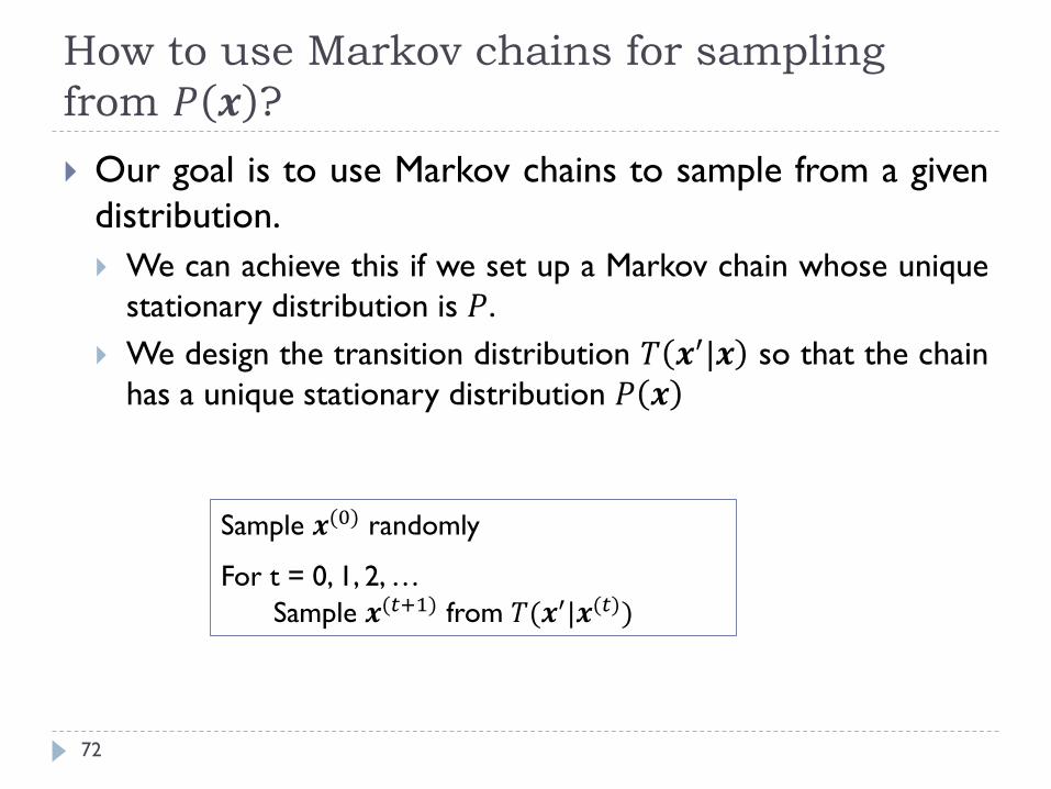
How to use Markov chains for sampling
from 𝑃 𝒙 ?
72
Our goal is to use Markov chains to sample from a given
distribution.
We can achieve this if we set up a Markov chain whose unique
stationary distribution is 𝑃.
We design the transition distribution 𝑇 𝒙′|𝒙 so that the chain
has a unique stationary distribution 𝑃 𝒙
Sample 𝒙(0) randomly
For t = 0, 1, 2, …
Sample 𝒙(𝑡+1) from 𝑇(𝒙′|𝒙(𝑡))
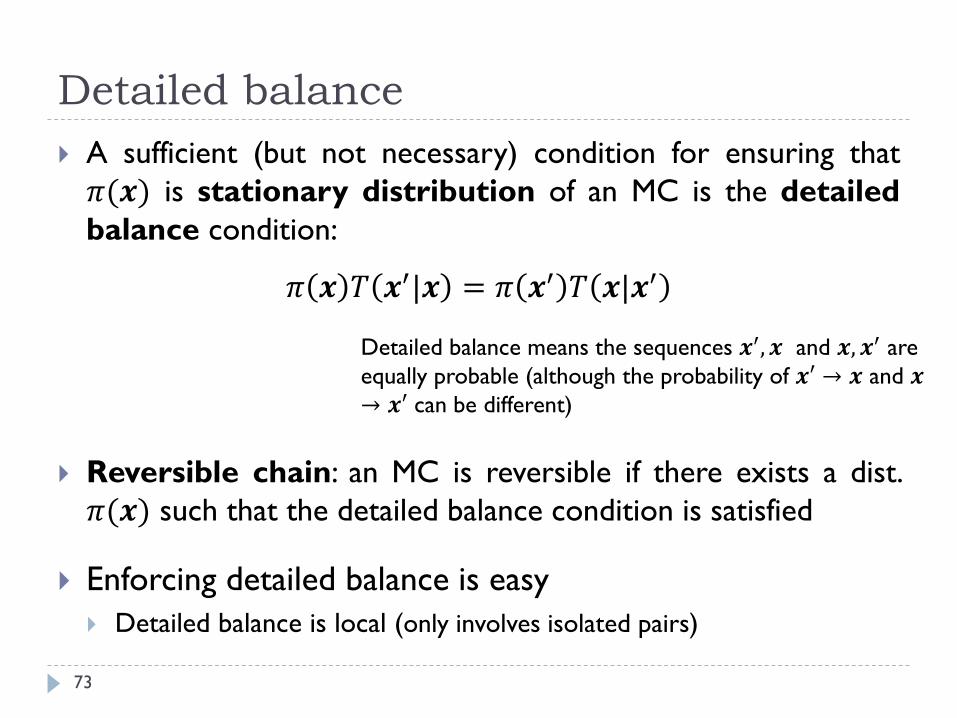
Detailed balance
73
A sufficient (but not necessary) condition for ensuring that
𝜋(𝒙) is stationary distribution of an MC is the detailed
balance condition:
𝜋 𝒙 𝑇 𝒙′|𝒙 = 𝜋 𝒙′ 𝑇 𝒙|𝒙′
Reversible chain: an MC is reversible if there exists a dist.
𝜋(𝒙) such that the detailed balance condition is satisfied
Enforcing detailed balance is easy
Detailed balance is local (only involves isolated pairs)
Detailed balance means the sequences 𝒙′, 𝒙 and 𝒙, 𝒙′ are
equally probable (although the probability of 𝒙′ → 𝒙 and 𝒙→ 𝒙′ can be different)
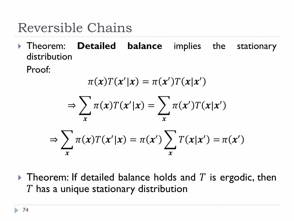
Reversible Chains
74
Theorem: Detailed balance implies the stationarydistribution
Proof:
𝜋 𝒙 𝑇 𝒙′|𝒙 = 𝜋 𝒙′ 𝑇 𝒙|𝒙′
⇒
𝒙
𝜋 𝒙 𝑇 𝒙′|𝒙 =
𝒙
𝜋 𝒙′ 𝑇 𝒙|𝒙′
⇒
𝒙
𝜋 𝒙 𝑇 𝒙′|𝒙 = 𝜋 𝒙′
𝒙
𝑇 𝒙|𝒙′ = 𝜋 𝒙′
Theorem: If detailed balance holds and 𝑇 is ergodic, then𝑇 has a unique stationary distribution


