Approximate solution to the Callan-Giddings-Harvey-Strominger field equations for two-dimensional evaporating black holes Amos Ori Department of Physics, Technion-Israel Institute of Technology, Haifa 32000, Israel (Received 27 July 2010; published 3 November 2010) Callan, Giddings, Harvey, and Strominger (CGHS) previously introduced a two-dimensional semi- classical model of gravity coupled to a dilaton and to matter fields. Their model yields a system of field equations which may describe the formation of a black hole in gravitational collapse as well as its subsequent evaporation. Here we present an approximate analytical solution to the semiclassical CGHS field equations. This solution is constructed using the recently introduced formalism of flux-conserving hyperbolic systems. We also explore the asymptotic behavior at the horizon of the evaporating black hole. DOI: 10.1103/PhysRevD.82.104009 PACS numbers: 04.70.Dy, 04.60.Kz I. INTRODUCTION The semiclassical theory of gravity treats spacetime geometry at the classical level but allows quantum treat- ment of the various fields which reside in spacetime. This theory asserts that a quantum field living on a black-hole (BH) background will usually be endowed with nontrivial fluxes of energy-momentum. These fluxes, represented by the renormalized stress-energy tensor ^ T , originate from the field’s quantum fluctuations, and typically they do not vanish even in the (incoming) vacuum state. The Hawking radiation [1], and the consequent BH evaporation, are perhaps the most dramatic manifestations of these quan- tum fluxes. In the framework of semiclassical gravity the spacetime reacts to the quantum fluxes via the Einstein equations, which now receive the extra quantum contribution ^ T at their right-hand side. The mutual interaction between ge- ometry and quantum fields thus takes its usual general- relativistic schematic form: The renormalized stress- energy tensor ^ T (say, in the vacuum state) is dictated by the background geometry, and the latter is affected by ^ T through the Einstein equations. In principle, this evo- lution scheme allows systematic investigation of the space- time of an evaporating BH. It turns out, however, that the calculation of ^ T ðxÞ for a prescribed background metric g ðxÞ is an extremely hard task in four dimensions. Nevertheless, in two-dimensional (2D) gravity the situation is remarkably simpler. There are two energy-momentum conservation equations, and the trace ^ T is also known (the ‘‘trace-anomaly’’). These three pieces of information are just enough for determining the three unknown components of ^ T . It is therefore possible to implement the evolution scheme outlined above in 2D gravity, and to formulate a closed system of field equations which describe the combined evolution of both spacetime and quantum fields. Callan, Giddings, Harvey, and Strominger (CGHS) [2] introduced a formalism of 2D gravity in which the metric is coupled to a dilaton field 0 and to a large number N of identical massless scalar fields. They added to the clas- sical action an effective term / N which gives rise to the semiclassical trace-anomaly contribution, and thereby automatically incorporates the renormalized stress-energy tensor ^ T into spacetime dynamics. The evolution of spacetime and fields is then described by a closed system of field equations. They considered the scenario in which a BH forms in the gravitational collapse of a thin massive shell, and then evaporates by emitting Hawking radiation. Their main goal was to reveal the end state of the evapo- ration process, in order to address the information puzzle. The general analytical solution to the CGHS field equa- tions is not known. Nevertheless, these equations can be explored analytically [3] as well as numerically [4–6]. The global structure which emerges from these studies is de- picted in Fig. 1: The shell collapse leads to the formation of a BH. A spacelike singularity forms inside the BH, at a certain critical value of the dilaton [3]. (The BH interior may be identified as the set of all events from which all future-directed causal curves hit the singularity.) The BH interior and exterior are separated by an outgoing null ray, which serves as an event horizon. Also an apparent horizon forms along a timelike line outside the BH (it is charac- terized by a local minimum of R e 20 along outgoing null rays). The event and apparent horizons are denoted by ‘‘EH’’ and ‘‘AH’’ in Fig. 1. Both horizons steadily ‘‘shrink’’ in time (namely, R decreases), exhibiting the BH evaporation process. At a certain point the apparent horizon intersects with the spacelike singularity (and with the event horizon). This intersection event (denoted ‘‘P’’ in Fig. 1) appears to be a naked singularity, visible to far asymptotic observers. It may be regarded as the ‘‘end of evaporation’’ point. The spacelike singularity which develops inside a CGHS evaporating BH was first noticed by Russo, Susskind, and Thorlacius [3]. Its local structure was recently studied in some detail [7], by employing the homogeneous approxi- mation. This singularity marks the boundary of predict- ability of the semiclassical CGHS formalism. About two PHYSICAL REVIEW D 82, 104009 (2010) 1550-7998= 2010=82(10)=104009(17) 104009-1 Ó 2010 The American Physical Society
Transcript
Approximate solution to the Callan-Giddings-Harvey-Stromingerfield equations for two-dimensional evaporating black holes
Amos Ori
Department of Physics, Technion-Israel Institute of Technology, Haifa 32000, Israel(Received 27 July 2010; published 3 November 2010)
Callan, Giddings, Harvey, and Strominger (CGHS) previously introduced a two-dimensional semi-
classical model of gravity coupled to a dilaton and to matter fields. Their model yields a system of field
equations which may describe the formation of a black hole in gravitational collapse as well as its
subsequent evaporation. Here we present an approximate analytical solution to the semiclassical CGHS
field equations. This solution is constructed using the recently introduced formalism of flux-conserving
hyperbolic systems. We also explore the asymptotic behavior at the horizon of the evaporating black hole.
The semiclassical theory of gravity treats spacetimegeometry at the classical level but allows quantum treat-ment of the various fields which reside in spacetime. Thistheory asserts that a quantum field living on a black-hole(BH) background will usually be endowed with nontrivialfluxes of energy-momentum. These fluxes, represented by
the renormalized stress-energy tensor T��, originate from
the field’s quantum fluctuations, and typically they do notvanish even in the (incoming) vacuum state. The Hawkingradiation [1], and the consequent BH evaporation, areperhaps the most dramatic manifestations of these quan-tum fluxes.
In the framework of semiclassical gravity the spacetimereacts to the quantum fluxes via the Einstein equations,
which now receive the extra quantum contribution T�� at
their right-hand side. The mutual interaction between ge-ometry and quantum fields thus takes its usual general-relativistic schematic form: The renormalized stress-
energy tensor T�� (say, in the vacuum state) is dictated
by the background geometry, and the latter is affected by
T�� through the Einstein equations. In principle, this evo-
lution scheme allows systematic investigation of the space-time of an evaporating BH.
It turns out, however, that the calculation of T��ðxÞ for aprescribed background metric g��ðxÞ is an extremely hard
task in four dimensions. Nevertheless, in two-dimensional(2D) gravity the situation is remarkably simpler. There aretwo energy-momentum conservation equations, and the
trace T�� is also known (the ‘‘trace-anomaly’’). These three
pieces of information are just enough for determining the
three unknown components of T��. It is therefore possible
to implement the evolution scheme outlined above in 2Dgravity, and to formulate a closed system of field equationswhich describe the combined evolution of both spacetimeand quantum fields.
Callan, Giddings, Harvey, and Strominger (CGHS) [2]introduced a formalism of 2D gravity in which the metric is
coupled to a dilaton field � and to a large number N ofidentical massless scalar fields. They added to the clas-sical action an effective term / N which gives rise to thesemiclassical trace-anomaly contribution, and therebyautomatically incorporates the renormalized stress-energy
tensor T�� into spacetime dynamics. The evolution of
spacetime and fields is then described by a closed systemof field equations. They considered the scenario in which aBH forms in the gravitational collapse of a thin massiveshell, and then evaporates by emitting Hawking radiation.Their main goal was to reveal the end state of the evapo-ration process, in order to address the information puzzle.The general analytical solution to the CGHS field equa-
tions is not known. Nevertheless, these equations can beexplored analytically [3] as well as numerically [4–6]. Theglobal structure which emerges from these studies is de-picted in Fig. 1: The shell collapse leads to the formation ofa BH. A spacelike singularity forms inside the BH, at acertain critical value of the dilaton [3]. (The BH interiormay be identified as the set of all events from which allfuture-directed causal curves hit the singularity.) The BHinterior and exterior are separated by an outgoing null ray,which serves as an event horizon. Also an apparent horizonforms along a timelike line outside the BH (it is charac-terized by a local minimum of R � e�2� along outgoingnull rays). The event and apparent horizons are denoted by‘‘EH’’ and ‘‘AH’’ in Fig. 1. Both horizons steadily‘‘shrink’’ in time (namely, R decreases), exhibiting theBH evaporation process. At a certain point the apparenthorizon intersects with the spacelike singularity (and withthe event horizon). This intersection event (denoted ‘‘P’’ inFig. 1) appears to be a naked singularity, visible to farasymptotic observers. It may be regarded as the ‘‘end ofevaporation’’ point.The spacelike singularity which develops inside a CGHS
evaporating BH was first noticed by Russo, Susskind, andThorlacius [3]. Its local structure was recently studied insome detail [7], by employing the homogeneous approxi-mation. This singularity marks the boundary of predict-ability of the semiclassical CGHS formalism. About two
PHYSICAL REVIEW D 82, 104009 (2010)
1550-7998=2010=82(10)=104009(17) 104009-1 � 2010 The American Physical Society
years ago Ashtekar, Taveras and Varadarajan [8] proposeda quantized version of the CGHS model, in which thedilaton and metric are elevated to quantum operators. Thisquantum formulation of the problem seems to resolve thesemiclassical singularity inside the BH [8], and thereby toshed new light on the information puzzle. In a very recentpaper [9] we applied a more simplified, ‘‘minisuperspace-like’’, quantum approach to the spacetime singularityinside a CGHS evaporating BH. We obtained a (bounce-like) extension of semiclassical spacetime beyond thesingularity.
The goal of this paper is to construct an approximateanalytical solution to the semiclassical CGHS field equa-tions, which will satisfactorily describe the BH formationand evaporation. This approximate solution applies as longas the BH is macroscopic, and as long as the spacetimeregion in consideration is ‘‘macroscopic’’ too—namely, Ris sufficiently large (i.e., not too close to the singularity). Insuch macroscopic regions, the semiclassical effects areweak in a local sense. Our solution is ‘‘first-order accu-rate’’ in this local sense; namely, the local errors in thesecond-order field-equation operators (applied to the ap-proximate solution) are quadratic in the magnitude of localsemiclassical effects (this is further discussed in Sec. VIII).
The method we use here for constructing our approxi-mate solution is based on the formalism of flux-conservingsystems [10]. This formalism deals with a special class ofsemilinear second-order hyperbolic systems in two dimen-sions. This class was first introduced in Ref. [11], and wassubsequently explored more systematically in Ref. [12]
(see also [13]). In particular, a flux-conserving hyperbolicsystem admits a rich family of single-flux solutions, towhich we refer as Vaidya-like solutions (see Sec. III), andfor which the field equations reduce to an ordinary differ-ential equation (ODE). Very recently we demonstrated [10]that after transforming to new field variables, the semiclas-sical CGHS equations take a form which is approximatelyflux-conserving. Here we take advantage of this propertyand use the formalism of flux-conserving systems to con-struct the approximate analytic solution to the CGHS fieldequations.Our approximate solution is presented in Sec. VI. It
involves a single function denoted by H, which is definedthrough a certain ODE. In order to make practical use ofthis approximate solution, one must have at his or herdisposal the solution for this ODE. In Appendix A weprovide an approximate analytical solution to this ODE.In Sec. II we briefly summarize the CGHS model, ex-
pressing the semiclassical field equations in convenientvariables R, S (already used in Refs. [7,10,11]). In particu-lar we discuss the classical model of a collapsing shell—which in fact provides the initial conditions to the semi-classical problem of BH evaporation. In Sec. III we intro-duce the new field variables ðW;ZÞ, which turn the fieldequations into a more standard form (with no first-orderderivatives). Then we observe the approximate flux-conserving system obtained in these new variables at thelarge-R limit. In Sec. IV we construct the ingoing Vaidya-like solution (a ‘‘single-flux’’ ingoing solution) of theflux-conserving system, which constitutes the core to ourapproximate solution. This core solution is complementedin Sec. V by adding to it a weak outgoing component. Theextra outgoing component must be added in order to cor-rectly satisfy the initial conditions at the collapsing shell(and it is this component which eventually gives rise to theoutgoing Hawking radiation). In Sec. VI we summarize ourapproximate solution, and also present an alternative ap-proximate expression for S. In Sec. VII we introduce twouseful gauges: the ‘‘shifted-Kruskal’’ gauge, and the semi-classical Eddington gauge. The validity of the constructedsolution is verified in Sec. VIII. We first describe themagnitude of the local error in the field equations, whichturns out to be quadratic in the local magnitude ofsemiclassical effects (assumed to be a small quantity).Subsequently we verify that the initial data at the collaps-ing shell are precisely matched by our approximatesolution, and the same for the initial data at past nullinfinity (PNI).In Sec. IX we discuss the horizon of the semiclassical
BH and a few related issues. The horizon (or ‘‘event-horizon’’) is the outgoing null line which separates theBH interior and exterior. We present the behavior of Rand S along the event horizon and also compute the influxTvv into the BH. We also discuss the location of theapparent horizon (defined by a minimum of R along an
FIG. 1. Penrose diagram describing the formation and evapo-ration of a two-dimensional CGHS black hole. The black holeforms by the collapse of a thin shell of macroscopic mass M0.The collapsing shell is located at v ¼ v0 � �M0=q. The linesdenoted ‘‘EH,’’ ‘‘AH,’’ and ‘‘CH,’’ respectively, represent theevent horizon, apparent horizon, and Cauchy horizon.
AMOS ORI PHYSICAL REVIEW D 82, 104009 (2010)
104009-2
outgoing null ray as mentioned above). Then in Sec. X weanalyze the asymptotic behavior at PNI, and also remarkbriefly on the asymptotic behavior at future null infinity(FNI). Finally, in Sec. XI we summarize our main results.
II. BACKGROUND: THE CGHS MODEL
A. Action and field equations
The CGHSmodel [2] consists of 2D gravity coupled to adilaton � and to a large number N � 1 of identical (free,minimally coupled, massless) scalar fields fi. Throughoutthis paper we express the metric in double-null coordinatesu, v for convenience, namely,
ds2 ¼ �e2�dudv: (1)
The action then takes the form
1
�
Zd2�
�e�2�ð�2�;uv þ 4�;u�;v � �2e2�Þ � 1
2
� XNi¼1
fi;ufi;v þ K�;u�;v
�; (2)
where K � N=12. The term �2 denotes a cosmo-logical constant. We shall set � ¼ 1 throughout. This isachieved by a change of variable � ! �0 ¼ �þ lnð�Þ,which annihilates � but does not affect the field equationsotherwise. This setting actually amounts to a choice ofbasic length unit.
The scalar fields all satisfy the trivial field equation
fi;uv ¼ 0: (3)
The CGHS scenario consists of an imploding thin massiveshell of mass M0 which moves along an ingoing null linev ¼ const � v0, forming a black hole. This shell is com-posed of (v derivatives of) the scalar fields fi, which areconcentrated as a �-function-like distribution at v ¼ v0.The solution at v < v0 is the trivial, flat, vacuum solution(see below). The main objective of this paper is the semi-classical solution which takes place at v > v0. By assump-tion, in this region too no incoming scalar waves arepresent. Therefore the solution of Eq. (3) throughout therelevant domain v > v0 (as well as at v < v0) is
fiðu; vÞ ¼ 0: (4)
The remaining field equations consist of two evolutionequations for the fields �, �, as well as two constraintequations (see [2]). To bring these equations to a simplerform we define new field variables
R � e�2�; S � 2ð���Þ; (5)
following Ref. [11]. The field equations for R and S thentake the form
R;uv ¼ �eS � K�;uv; (6)
S;uv ¼ K�;uv=R; (7)
where
� ¼ ðS� lnRÞ=2 (8)
is to be substituted. The constraint equations become (aftersubstituting fi ¼ 0 for the scalar fields)
R;uu � R;uS;u þ Tuu ¼ 0; (9)
R;vv � R;vS;v þ Tvv ¼ 0; (10)
where Tuu; Tvv are the semiclassical fluxes in the two nulldirections, given by
T uu ¼ K½�;uu � �2;u þ zuðuÞ�; (11)
T vv ¼ K½�;vv � �2;v þ zvðvÞ�: (12)
The functions zuðuÞ, zvðvÞ are initial functions whichencode the information about the system’s quantum state.Following CGHS we consider here an incoming vacuumstate at PNI (apart from the imploding massive shell, whichis presumably encoded in the fields fi already at theclassical level). Correspondingly the functions zuðuÞ,zvðvÞ are determined by the requirement that Tuu and
Tvv vanish at PNI.1
It will sometimes be useful to reexpress the system ofevolution Eqs. (6) and (7) in its standard form, in whichR;uv and S;uv are explicitly given in terms of lower-order
derivatives:
R;uv ¼ �eS2R� K
2ðR� KÞ � R;uR;v
K
2RðR� KÞ ; (13)
S;uv ¼ eSK
2RðR� KÞ þ R;uR;v
K
2R2ðR� KÞ : (14)
This form makes it obvious that the evolution equationsbecome singular when R ¼ K, and also at R ¼ 0. Thissingularity was studied in some detail in Ref. [7].
Gauge freedom
In a coordinate transformation u ! u0ðuÞ, v ! v0ðvÞ thedilaton scalar field � is unchanged, but � changes as
1In a 2D spacetime there are two sectors of PNI, a ‘‘right PNI’’and a ‘‘left PNI’’. zuðuÞ is defined by the demand Tuu ¼ 0 at leftPNI, and zvðvÞ by demanding Tvv ¼ 0 at right PNI. Similarlythere are two sectors of FNI, a right one and a left one.Throughout this paper, by ‘‘PNI’’ and ‘‘FNI’’ we shall alwaysrefer to the right sectors of PNI and FNI (unless stated other-wise), as is also illustrated in Fig. 1.
APPROXIMATE SOLUTION TO THE CALLAN-GIDDINGS- . . . PHYSICAL REVIEW D 82, 104009 (2010)
104009-3
�0 ¼ �� 1
2
�lndu0
duþ ln
dv0
dv
�(15)
[as may be deduced from the coordinate transformationof the metric component guv ¼ �ð1=2Þe2�]. From thedefinition (5) of R and S it is obvious that R is a scalar,and S changes in a coordinate transformation like 2�:
R0 ¼ R; S0 ¼ S� lndu0
du� ln
dv0
dv: (16)
Below we shall often provide expressions for S in certainspecific gauges. In such cases we shall use the notationS½...�, with the specific u, v coordinates specified in the
square brackets. The same notation will apply to � (andalso to the gauge-dependent quantity Z introduced in thenext section).
B. Classical solutions
The classical solutions are obtained by setting K ¼ 0,
leading to Tuu ¼ Tvv ¼ 0. The vacuum field equationsthen reduce to the evolution equations
R;uv ¼ �eS; S;uv ¼ 0 (17)
and the constraint equations
R;uu � R;uS;u ¼ R;vv � R;vS;v ¼ 0: (18)
The general solution of these equations may be easilyconstructed. It takes the form
where M is an arbitrary constant, and RuðuÞ and RvðvÞ areany monotonically increasing functions of their arguments(with nonvanishing derivatives). The classical solutionmay thus look at first glance as a rich class depending ontwo arbitrary functions. However, these two functionsmerely reflect the gauge freedom. To fix this freedom wemay use the Kruskal-like coordinates U � RuðuÞ, V �RvðvÞ, after which the general solution takes the simpleexplicit form
R ¼ M�UV; S½U;V� ¼ 0: (20)
The subindex ‘‘½U;V�,’’ recall, indicates that this expres-sion for S only applies in a specific gauge, the one asso-ciated with the Kruskal U, V coordinates.
The representation (20) makes it obvious that theclassical vacuum solution is a one-parameter family, pa-rametrized by the mass M. We shall refer to it as theSchwarzschild-like solution.
For M> 0 the spacetime contains a BH, whosecausal structure resembles that of the four-dimensionalSchwarzschild spacetime (see [2]). The event horizon islocated atU ¼ 0, and the past (or ‘‘white-hole’’) horizon atV ¼ 0. Inside the BH (U, V > 0) there is a spacelike R ¼ 0singularity (�, � diverge) at UV ¼ M. For negative M
there is a naked, timelike, R ¼ 0 singularity instead of aBH. (The M ¼ 0 case is considered below.)Another useful gauge is the Eddington-like gauge, ob-
tained by the transformation2
ue � � lnð�UÞ; ve � lnV ðU < 0; V > 0Þ:(21)
The solution then takes the form
R ¼ Mþ eve�ue ; S½ue;ve� ¼ ve � ue: (22)
Note that these coordinates only cover the BH exterior.Analogous Eddington-like coordinates (with appropriatesign changes) may also be constructed for the BH interior,but we shall not need these internal coordinates here.The special case M ¼ 0 yields the Minkowski-like so-
lution. In Kruskal coordinates it takes the form
R ¼ �UV; S½U;V� ¼ 0: (23)
In Eddington coordinates one obtains R ¼ eve�ue ,S½ue;ve� ¼ ve � ue, and hence �½ue;ve� ¼ 0. This demon-
strates that the M ¼ 0 solution is flat, and also indicatesthat the Eddington-like coordinates ðue; veÞ correspond inthis case to the standard, flat, null coordinates of 2DMinkowski spacetime.In the general case M � 0 one finds from
Eqs. (22) and (8)
�½ue;ve� ¼ � 1
2ln
�1þ M
eve�ue
�; (24)
and the associated metric ds2 ¼ �e2�dudv yields non-vanishing curvature. However, at large ve � ue this ex-pression reduces to
�½ue;ve� ffi � M
2eve�ueffi � M
2R; (25)
which vanishes as ve � ue ! 1. That is, in Eddingtoncoordinates � vanishes at (right) PNI (ue ! �1), FNI(ve ! 1), and spacelike infinity (ue ! �1, ve ! 1).The Schwarzschild-like solution is thus asymptoticallyflat, and ðue; veÞ serve as asymptotically flat coordinatesin this spacetime. In particular, ve and ue respectivelycoincide with the affine parameter along PNI and FNI.
1. Classical collapsing shell
The physical scenario which concerns us here is theformation of a BH by the collapse of a thin shell, carryinga mass M0 > 0, which propagates along an ingoing nullline v ¼ v0. The classical solution describing this scenario
2The coordinate ue introduced here is the classical outgoingEddington coordinate. It should not be confused with the semi-classical outgoing Eddington coordinate ~u introduced inSec. VII. On the other hand the ingoing Eddington coordinateve (denoted later by v) is common to the classical and semi-classical solutions.
AMOS ORI PHYSICAL REVIEW D 82, 104009 (2010)
104009-4
is obtained by continuously matching a Minkowski-likesolution at v � v0 with a Schwarzschild-like solution atv � v0. To describe the matching we start with the Kruskalgauge solution (20), along with its M ¼ 0 analog (23).Obviously the R functions in these two expressions donot properly match (at any V). To allow for continuousmatching, we shift the U coordinate in the Minkowski-like
domain v < v0, defining U � Uþ�U, where �U is aconstant. Note that S is unchanged in this coordinate trans-formation. We obtain the Minkowski-like solution in itsnew form:
R ¼ ð�U� UÞV; S½U;V� ¼ 0 ðv < v0Þ: (26)
This solution can now be matched to Eq. (20), by equating
V�U to M0 at the null shell. Omitting the hat from U andrenaming this new Minkowski-like Kruskal coordinate byU, we obtain the matched solution
S½U;V� ¼ 0; RðU;VÞ ¼� ð�U�UÞV V < V0
M0 �UV V > V0;
(27)
where V0 is the shell’s V value (we assume V0 > 0), andcontinuity implies �U ¼ M0=V0.
To formulate the semiclassical initial data (next subsec-tion) we find it most convenient to work with Eddingtonv and Kruskal U. The collapsing-shell solution then takesthe form
S½U;ve� ¼ ve; RðU; veÞ ¼� ð�U�UÞeve ve < v0
e
M0 �Ueve ve > v0e;
(28)
where v0e � lnV0.
2. Fixing the v gauge
Throughout the semiclassical analysis below, we findthe Eddington ve to be the most convenient v coordinate,and no other v coordinate will be used. To simplify thenotation, in the rest of this paper we shall simply denote ve
by v.For the u gauge we shall occasionally use several u
coordinates at various stages of the construction. The valueof S (like � and Z) in specific u gauges will be denotedby S½...�—with the specific u coordinate only specified in
the squared brackets—and it will always refer to theEddington v coordinate. No confusion should arise, be-cause no v coordinate other than Eddington will be usedthroughout the rest of the paper.
To practice the new notational rules we rewrite the aboveclassical collapsing-shell solution (28) in the new notation:
S½U� ¼ v; RðU; vÞ ¼� ð�U�UÞev v < v0
M0 �Uev v > v0;(29)
where v0 ¼ lnV0 denotes the shell’s location inEddington-v, and
�U ¼ M0e�v0 :
The collapsing-shell spacetime (29) is asymp-totically flat, just like the pure Schwarzschild-like andMinkowski-like solutions. Also, the Eddington coordinatev serves as an affine parameter at PNI. [This may beverified by switching to the Eddington coordinate ue �� lnð�UÞ and noting that �½ue� vanishes at the PNI limit
ue ! �1.]
C. Initial data for the semiclassical solution
1. Initial conditions at the Shell
We return now to the semiclassical problem of collaps-ing shell. The semiclassical effects vanish at the portionv < v0 of the collapsing-shell spacetime, owing to itsflatness.3 Therefore, the portion v < v0 is correctly de-scribed by Eq. (29) even in the semiclassical problem.The portion v > v0 of the collapsing-shell spacetime
will be profoundly modified by semiclassical effect(as expressed, for example, by the BH evaporation).However, by continuity, the initial conditions for R and Sat v ¼ v0 will still be determined by matching to the same,unmodified, Minkowski-like solution at v < v0, and willtherefore be exactly the same as in the classical solution(29). Using again the Kruskal-U coordinate (and, recall,the Eddington-v coordinate as usual), these shell initialconditions take the form
R0ðUÞ � RðU; v0Þ ¼ M0 �Uev0 (30)
and
S½U�0 ðUÞ � S½U�ðU; v0Þ ¼ v0: (31)
2. Initial conditions at past null infinity
The semiclassical evolution equations (6) and (7) alsorequire initial conditions at an outgoing null ray, which ismost conveniently taken to be the PNI boundary. Thesituation here is somewhat similar to that of the initialdata at the shell: Owing to asymptotic flatness of thecollapsing-shell spacetime [and to the lack of any strong-field region at the causal past of PNI (unlike the situation atFNI)], the asymptotic behavior at PNI is just the classicalone. Specifically one finds the initial conditions
R ffi M0 �Uev; S½U� ffi v ðPNIÞ (32)
in the domain v > v0. In particular, the influx Tvv shouldvanish at PNI (corresponding to an incoming vacuumstate).
3Flatness means that the term �;uv in the semiclassical evolu-tion equations (6) and (7) vanishes, so these equations reduce tothe classical ones.
APPROXIMATE SOLUTION TO THE CALLAN-GIDDINGS- . . . PHYSICAL REVIEW D 82, 104009 (2010)
104009-5
D. The role of K in semiclassical dynamics
The semiclassical effects originate from the last termK�;u�;v in the CGHS action (2). The parameterK ¼ N=12thus determines the overall magnitude of semiclassicaleffects. It is important to note, however, that K may befactored out from CGHS dynamics by a simple shift/rescaling of variables. In the transformation
N ! cN; K ! cK; � ! �� 1
2lnc (33)
[with �, �, and fi unchanged (and with all scalar fields fiidentical)], the action is merely multiplied by c; hence thefield equations are unaffected. One can therefore factor outK this way by choosing c ¼ 1=K.
In the relevant domain v > v0 the scalar fields fi vanishanyway, so the term � 1
2
PNi¼1 fi;ufi;v is absent from the
action (2). In terms of the new variables R, S, the rescalinglaw takes the form
K ! cK; R ! cR; S ! Sþ lnc: (34)
This scaling makes it obvious that the relative magnitudeof semiclassical effects in various regions of spacetime willnot be determined by K or R separately, but only through(dimensionless4) combinations like K=R or K=eS, whichare invariant to the rescaling.5
One can easily verify that in the above scaling trans-formation the BH original massM0 is multiplied by c. It isa common wisdom that when a BH is macroscopic, semi-classical effects will be locally weak6 (except in the neigh-borhood of the singularity). The above scaling lawmakes itobvious that whether a BH may be regarded as macro-scopic or not would only depend on the ratio ofM0 and K:A CGHS BH should be regarded as macroscopic ifM0 � K—which we indeed assume throughout this paper.
In principle, the above scaling allows us to set K ¼ 1 inthe field equations. We find it more convenient, however, to
leave K in the equations untouched. The parameter Kserves as a ‘‘flag’’ marking the terms of semiclassicalorigin in the various equations. Also, in the equationsbelow K always appears through combinations like K=R,K=R0, K=M0 (or sometimes with R replaced by the vari-able W R introduced below). We shall assume through-out this paper that the BH is macroscopic (M0 � K), anddeal with spacetime regions satisfying R � K. This willallow us to expand various expressions to first order insmall quantities such as K=R or alike. All these expansionsmay conveniently be handled formally as expansions in K(or in the parameter q ¼ K=4 introduced below)—thoughone should bear in mind that the small parameter in theexpansion is not K itself, but the combinations K=R,K=M0, etc.
III. FIELD REDEFINITION AND FLUX-CONSERVING FORMULATION
A. Field redefinition
The evolution equations (6) and (7) may look quitesimple at first glance. However, to close the system onemust substitute Eq. (8) for �, which makes the equationsrather messy. Bringing these equations to their standardform, one ends up with Eqs. (13) and (14). In addition totheir rather complicated form, these second-order equa-tions also have the inconvenient property of being explic-itly dependent on first-order derivatives R;u, R;v.
To get rid of this undesired dependence upon R;u and
R;v, we transform from R and S to new variables W, Zdefined by [14]
With these new variables the evolution equations take theschematically simpler form:
W;uv ¼ eZVWðWÞ; Z;uv ¼ eZVZðWÞ; (38)
with certain ‘‘potentials’’ VWðWÞ and VZðWÞ. But thesimplification does not come without a cost: These poten-tials are explicitly obtained as functions of R rather thanW.One finds
4Note that after � is set to 1 [see discussion following Eq. (2)]all the model’s quantities become dimensionless. This includesR, and also the BH mass M0. (The latter is naturally linked toR—for example, through the horizon’s R value.)
5It is important not to confuse here between two differentissues related to the magnitude of K: First, whether the semi-classical treatment is applicable or not. Second, within thesemiclassical formulation, K determines the magnitude of semi-classical effects. CGHS pointed out [2] that the semiclassicaltreatment is only valid if K � 1. Here we address the secondissue. Namely, we assume that the condition K � 1 is satisfied,and explore the scaling law which characterizes the magnitude ofsemiclassical effects (and its relation to the scale of othervariables like R).
6Here, again, it is important to distinguish between two differ-ent aspects of ‘‘macroscopicality’’: (i) whether the semiclassicaltheory is applicable to the BH evaporation and (ii) whether,within the semiclassical formulation, the semiclassical effectsare locally weak. The discussion here pertains to the secondaspect. To satisfactorily deal with (i) one has to further assumeK � 1 (see also previous footnote).
Despite this disadvantage, the form (38) allows an effectivetreatment of the semiclassical dynamics, as will be dem-onstrated below.
Notice that the gauge transformation (16) of R and Scarries over to W and Z, respectively:
W 0 ¼ W; Z0 ¼ Z� lndu0
du� ln
dv0
dv: (41)
The value of Z in a specific u gauge will be denoted byZ½...�, in full analogy with our notation for S.
B. Large-R asymptotic behavior
From now on we shall consider a macroscopic BH,M0 � K, and restrict the analysis to spacetime regionswhere R � K. We expand Eqs. (35) and (37) to first orderin the small quantity K=R:
W ¼ R
�1� K
2RlnRþO
�K
R
�2�; (42)
�Z ¼ � K
4RþO
�K
R
�2: (43)
The inverse function RðWÞ is given at this order by
R ¼ W
�1þ K
2WlnW þO
�K
W
�2�: (44)
The potentials VWðWÞ; VZðWÞ can now easily be expandedto first order in K=W,
VW ¼ �1� K
4WþO
�K
W
�2;
VZ ¼ 1
W
�K
4WþO
�K
W
�2�:
(45)
C. The flux-conserving system
We now proceed with the above large-R approximation,keeping only terms up to first order in K=R (or K=W); thuswe analyze the hyperbolic system
W;uv ¼ eZVWðWÞ; Z;uv ¼ eZVZðWÞ (46)
with
VW ¼ �1� q
W; VZ ¼ q
W2; (47)
where
q � K
4:
Since VZ ¼ dVW=dW, Eqs. (46) and (47) constitute aflux-conserving system. This concept was first introducedin Ref. [11] and was later described in more detail inRefs. [10,12]. Our system corresponds to F ¼ VW ¼�1� q=4; hence the generating function [15] is
h0ðWÞ ¼ W þ q lnW: (48)
In conjunction with the system (46) and (47), we shallalso use the transformation between ðR; SÞ and ðW;ZÞchopped at first order in q, namely,
W ¼ R� 2q lnR; (49)
R ¼ W þ 2q lnW; (50)
Z ¼ S� q
R¼ S� q
W; (51)
S ¼ Zþ q
R¼ Zþ q
W: (52)
We also rewrite here the shell initial conditions (30) and(31) in the new variables W and Z, to first order in q:
W0ðUÞ � WðU; v0Þ ¼ R0 � 2q lnR0 (53)
and
Z½U�0 ðUÞ � Z½U�ðU; v0Þ ¼ v0 � q
R0
: (54)
1. Ingoing Vaidya-like solutions
Like any flux-conserving system, the system (46) and(47) admits Vaidya-like solutions—namely, solutions witha single flux [15]. Each Vaidya-like solution is endowedwith a mass function—a function of one of the null coor-dinates which encodes the information about the flux. As itturns out, at the leading order an evaporating BH may beapproximated by an ingoing Vaidya-like solution with alinearly decreasing mass function. [However, a first-orderoutgoing component has to be superposed on it in order toprecisely match the initial conditions, as we discuss be-low.] Assuming that the BH was created by the collapse ofa shell of mass M0, which propagated along the null orbitv ¼ v0, the appropriate mass function takes the form�MðvÞ ¼ M0 � qðv� v0Þ. This choice is motivated by thewell-known fact [2] that a 2D macroscopic BH evaporatesat a constant rate q ¼ N=48, and the suitability of (theapproximate solution derived from) this mass function isverified in Sec. VIII below. By shifting the origin of v suchthat v0 ¼ �M0=q, we obtain the mass function in a morecompact form:
�MðvÞ ¼ �qv � mvðvÞ: (55)
The restriction to a Vaidya-like solution leads to a greatsimplification, because the problem now reduces to that ofsolving an ODE (rather than a system of partial differentialequations). Thus, as described in Ref. [10],Wðu; vÞ is nowdetermined from the ODE W;v ¼ h0ðWÞ � �MðvÞ (appliedalong each line u ¼ const), or, more explicitly,
W;v ¼ ðW þ q lnWÞ þ qv: (56)
The other unknown Zðu; vÞ is then given by
Z ¼ lnð�W;uÞ: (57)
Alternatively [10] Z may be obtained from the ODE
Z;v ¼ 1þ q
W: (58)
APPROXIMATE SOLUTION TO THE CALLAN-GIDDINGS- . . . PHYSICAL REVIEW D 82, 104009 (2010)
104009-7
As was mentioned above, we set the origin of v such thatthe collapsing shell is placed at v0 ¼ �M0=q. Thereforethe parameter v0 is negative. Also, throughout this paperwe assume that the BH is macroscopic, namely, M0 � q,and this implies v0 �1.
2. Weakly perturbed Vaidya-like solution
The above-mentioned ingoing Vaidya-like solution wellapproximates many aspects of the CGHS spacetime.However, it fails to precisely match the initial conditionsat the shell. This mismatch is small, / ðq=WÞ, yet it mustbe fixed in order to satisfactorily handle some of the moresubtle aspects of the solution (most importantly, theHawking outflux at FNI). Thus, we must fix the ingoingVaidya-like solution by adding to it a small outgoingcomponent, seeded by the mismatch at the shell.Nevertheless, owing to the small / ðq=WÞ magnitude ofthe mismatch, it will be possible to treat this outgoingcomponent as a small (linear) perturbation on top of theingoing Vaidya-like solution discussed above (to which weshall refer as the ‘‘core solution’’).
In the next section we shall proceed with analyzing theingoing Vaidya-like core solution. Then in Sec. V we shallconstruct the perturbing outgoing component and therebycomplete the construction of the approximate solution.
IV. CONSTRUCTING THE INGOINGVAIDYA-LIKE CORE SOLUTION
A. Processing the ODE for W and introducing H
The term q lnW in the right-hand side of Eq. (56) makesthis equation hard to analyze. In order to ease the analysiswe define the auxiliary variable H � W;v þ q, namely,
H ¼ W þ q lnW �mv þ q: (59)
The inverse functionWðHÞ cannot be expressed in a closedexact form; however, restricting the analysis to first orderin q we may use the relation
W ¼ Hþmv � q½lnðH þmvÞ þ 1�: (60)
Differentiating now H using Eq. (59) and W;v ¼ H � qwe find
H;v ¼ qþ @H
@WW;v ¼ qþ
�1þ q
W
�ðH � qÞ:
Further substituting Eq. (60) in the right-hand side andomitting all / q2 terms, we obtain the ODE for H in itsmore compact form:
H;v ¼ H
�1þ q
H � qv
�: (61)
The initial conditions for H is to be specified at theshell’s orbit, the line v ¼ v0 (this line serves as a character-istic initial surface for the nontrivial piece v > v0 of theCGHS spacetime). We denote it H0ðuÞ � Hðu; v0Þ. InSec. IVD we calculate H0 and show that it decreaseslinearly with the Kruskal coordinate U. Then in Sec. VII
we express H0ðuÞ in a few other useful gauges. Note thatthe dependence of H on u only emerges through the initialcondition H0ðuÞ. Correspondingly we shall often expressthis parametric dependence in the formHðv;uÞ, and some-times ignore it altogether and use the abbreviated notationHðvÞ, for convenience.We are unable to solve the ODE (61) analytically.
However, an approximate solution is given in Appendix A.Furthermore, several exact key properties of the solutionsof Eq. (61) are described below.Note the advantage of the ODE of H over Eq. (56) for
W;v, particularly at large H. The latter corresponds to
future or past null infinity, where, as it turns out, H (likeW) grows exponentially in v. The ODE then reduces to thetrivial oneH;v ffi H þ q, which is easily solved (leading tothe above-mentioned exponential growth). In the ODE forW, on the contrary, one faces the lnW term, which com-plicates the asymptotic behavior at future/past null infinity.
B. Some exact properties of Hðv;uÞGiven the ODE (61), the function Hðv; uÞ is uniquely
determined by the initial-value function H0ðuÞ � Hðu; v0Þ[this function is explicitly constructed below; cf. Eqs. (67)and (68)]. We therefore start our discussion here by men-tioning two key properties of H0ðuÞ which are importantfor the present analysis: First, H0ðuÞ is monotonicallydecreasing. It is positive at early u but becomes negativeafterwards. It vanishes at a certain u value which we denoteuhor (in Kruskal gauge it corresponds to U ¼ �qe�v0).Second, H0ðuÞ þM0 is positive at any u.We first note that the ODE (61) admits a trivial solution
HðvÞ ¼ 0. It immediately follows that H vanishes alongthe line u ¼ uhor (but nowhere else).Next, we define (off the line u ¼ uhor whereH vanishes)
lðv;uÞ � lnjHðv; uÞj: (62)
It satisfies the ODE
l;v ¼ 1þ q
H þmv
¼ 1þ q
�el � qv; (63)
where the ‘‘�’’ sign reflects the sign of H.Both Eqs. (63) and (61) develop a singularity whenever
Hþmv vanishes, but are regular otherwise. Since H0 þM0 > 0, the quantity H þmv is always positive at v ¼v0 and its neighborhood. In principle there could be twopossibilities, which may depend on u [through the initialvalue H0ðuÞ]: (i) Hðv;uÞ is regular throughout v > v0, or(ii) Hðv; uÞ becomes singular (H þmv vanishes) at acertain finite v ¼ vsingðuÞ> v0.
7 To treat both cases in
a unified manner we shall say that the solution Hðv;uÞis regular and well-defined throughout the domain
7As will become obvious later, option (i) occurs at u < uhor
and option (ii) at u > uhor.
AMOS ORI PHYSICAL REVIEW D 82, 104009 (2010)
104009-8
v0 � v < vfðuÞ, where vfðuÞ ¼ 1 in case (i) and
vfðuÞ ¼ vsingðuÞ in case (ii).
We can now deduce the following exact properties ofHðv; uÞ, which hold throughout the domain of regularityv < vfðuÞ:
(a) As was already mentioned above, H vanishes alongthe line u ¼ uhor. This holds throughout the rangev0 � v < 0. [At ðu ¼ uhor; v ! 0Þ the ODE be-comes singular because H þmv vanishes.] H can-not vanish at any other value of u, because otherwiseH0ðuÞ would have to vanish too at that specific u �uhor (which is not the case).
(b) Consequently,Hðu; vÞ has the same sign asH0ðuÞ atany u. As was mentioned above, this sign is positiveat u < uhor and negative at u > uhor. These twodomains are separated by the line u ¼ uhor on whichu vanishes.
(c) Since H þmv is positive at v ¼ v0, it remainspositive throughout v0 < v< vfðuÞ.
(d) Correspondingly, the right-hand side in Eq. (63) isstrictly positive, and in fact>1. Thus, lðvÞ is mono-tonically increasing, and the same for jHðvÞj.
(e) The quantity H;u satisfies the ODE
d
dvlnjH;uj ¼ 1� q2v
ðH þmvÞ2
[cf. Eq. (87)]. The right-hand side is regular at anyv < vfðuÞ, and positive throughout v � 0. Since
H0;u is negative for all u,8 it immediately follows
from this ODE that H;u is everywhere negative.
Furthermore, at least at v < 0, jH;uj is an increasingfunction of v; therefore, at fixed u (and v < 0)H;u is
bounded above by the parameter H0;u < 0.(f) The same obviously applies to ðH þmvÞ;u (in par-
ticular, this quantity is everywhere negative). It thenfollows that if a singularity H þmv ¼ 0 occurs atsome u ¼ u1 (with finite vsing > v0), then such a
singularity must occur at any u > u1, and vsingðuÞmust be a nonincreasing function of u (throughoutu > u1). Furthermore, in the range where vsingðuÞ<0 [see (g)], vsingðuÞ must be a strictly decreasing
function of u.(g) As was mentioned above, at u > uhor H0ðuÞ is nega-
tive, and the same for Hðv; uÞ. [Furthermore, sincejHðvÞj is monotonically increasing, at each line u ¼const in this domain H is bounded above by theparameter H0ðuÞ< 0.] It then follows that H þmv
(which is positive at v ¼ v0) must vanish beforemv
vanishes. Thus, all lines u > uhor run into an H þmv ¼ 0 singularity at a certain v ¼ vsingðuÞ< 0.
Property (f) then implies that vsing is a strictly
decreasing function of u, indicating that this is aspacelike singularity.
(h) In the domain u < uhor,H is strictly positive, and nosingularity may form at v � 0 (wheremv is positivetoo). However, at v > 0 mv is negative, and onemight be concerned about the possibility of vanish-ing H þmv, which would lead to a singularity. Acloser examination reveals that such a singularitydoes not occur in this domain. This may be deducedfrom each of the following arguments (though acomplete mathematical proof is still lacking): (i) Itis easy to show that at least a locally monotonicsingularity of this type (namely, a singularity ofvanishing H þmv at some finite v ¼ vsing, such
that H þmv is monotonic in v throughout someneighborhood of v ¼ vsing) is not possible in the
domain u < uhor: H þmv starts positive at v ¼ v0,and in order to vanish it must decrease on approach-ing v ¼ vsing. However, since H > 0 (and increas-
ing), when H þmv approaches zero from aboveEq. (61) yields H;v ! þ1, and therefore Hþmv
must increase, so it cannot vanish. It is harder tomathematically exclude the possibility of an oscil-latory approach to an Hþmv ¼ 0 singularity, butsuch an oscillatory behavior seems very unlikely.(ii) Consider the limiting function Hðv;uhor� Þ, de-fined to be the limit u ! uhor� of Hðv;uÞ. At v < 0this function vanishes, just like Hðv; uhorÞ, by con-tinuity. At v � 0 [where Hðv; uhorÞ is not defined;see (a)], this function becomes a nontrivial solutionof the ODE (61). Numerical examination shows thatHðv;uhor� Þ continuously increases from zero atv ¼ 0 to infinity at v ! 1, with H þmv > 0 atany v > 0. From (f) it now follows thatH þmv > 0throughout u < uhor. (iii) Direct numerical simula-tions of Hðv; uÞ at various u < uhor values furtherconfirm this conclusion.
Summarizing the above discussion on the exact proper-ties of Hðu; vÞ, and briefly restating it in more physical/geometrical terms: All lines u < uhor make it to FNI,whereas all lines u > uhor run into a spacelike singularity9
at v ¼ vsingðuÞ< 0.
Based on these causal properties of Hðu; vÞ and itssingularity, we shall refer to the ranges u < uhor and
8H0 decreases linearly with U, and we only consider here ugauges satisfying du=dU > 0.
9The exact semiclassical CGHS spacetime admits a verysimilar global structure: A BH, with a spacelike singularityinside it. We point out, however, that the local properties ofthe spacelike singularity in our approximate solution are differ-ent from those of the precise CGHS spacetime. In particular, inour approximate solution (when literally applied to the H þmv ¼ 0 singularity) R diverges logarithmically to �1, whereasin the CGHS solution R ¼ K at the singularity [7]. This remark-able difference is not a surprise, because the parameter q=R is nolonger small when we get close to the singularity, hence ourapproximate solution becomes invalid there.
APPROXIMATE SOLUTION TO THE CALLAN-GIDDINGS- . . . PHYSICAL REVIEW D 82, 104009 (2010)
104009-9
u > uhor as the BH exterior and interior, respectively. Notethat the interior is confined to the range v0 � v <
vsingðuÞ< 0 (and u > uhor), whereas the exterior extends
in the entire domain v0 � v <1 (for u < uhor).
C. Expressing the ingoing solution in terms of H
The function Hðu; vÞ may be obtained by solving theODE (61) numerically, or by analytic approximate solu-tions like the one given in Appendix A. Once H is known,W is given by Eq. (60), and Z in turn by Eq. (57). Theformer equation yields
W;u ¼�1� q
Hþmv
�H;u;
hence, up to first order in q,
Z ¼ lnð�H;uÞ � q
H þmv
: (64)
One can easily verify the consistency of this expressionwith the u-gauge transformation of Z, given in Eq. (41)(note that H is unchanged in such a transformation).
D. Calculating H0ðuÞTo calculate H0ðuÞ we evaluate Eq. (64) at v ¼ v0 and
equate it to the desired initial condition Z0ðuÞ. It is conve-nient to carry out this calculation in the Kruskal gauge.Using Eqs. (54) and (30) we obtain the following equationfor H0:
lnð�H0;UÞ � q
H0 þM0
¼ v0 � q
M0 �Uev0: (65)
A simple solution immediately suggests itself, H0 ¼�Uev0 , but we need here the general solution for thisODE, which spans a one-parameter family. For our pur-pose it will be sufficient, however, to derive an approxi-mate general solution (up to order q), which is an easy task.Such a one-parameter family of approximate solutions is
H0ðUÞ ¼ �Uev0 þ pq; (66)
where p is a yet-arbitrary constant. This constant may befixed by solving the ODE (61) for Hðv;UÞ in the PNIasymptotic limit [with the above expression for H0ðUÞ asinitial condition], constructingW, Z from H and then R, S,and comparing them to the desired initial data at PNI. InAppendix B we carry out this analysis and find that theappropriate value is p ¼ �1, namely,
H0ðUÞ ¼ �Uev0 � q: (67)
We may also use Eq. (30) to rewrite H0 in a form which isexplicitly gauge-invariant (for arbitrary u coordinate):
H0ðuÞ ¼ R0ðuÞ �M0 � q: (68)
V. THE WEAK PERTURBING OUTFLUX
The above ingoing Vaidya-like solution was constructed[through an appropriate choice of H0ðuÞ] such that itproperly matches the initial function Z0ðuÞ at the shell.However, the other initial function W0ðuÞ does not exactlycoincide withW of the above constructed ingoing solution.To fix this mismatch we shall add a weak, outgoing com-ponent as a perturbation on top of the ingoing coresolution.To this end we write the overall W, Z functions as
Wðu; vÞ ¼ Winðu; vÞ þ �Wðu; vÞ; (69)
Zðu; vÞ ¼ Zinðu; vÞ þ �Zðu; vÞ; (70)
where W in, Zin denote the Vaidya-like ingoing core solu-tion constructed in the previous section [namely, Eqs. (60)and (64)], and �W, �Z denote the additional perturbingcomponent.10
We first calculate the mismatch in the initial conditionfor W. Equations (60) and (67) yield for W in at the shell
W in0 ðUÞ ¼ M0 �Uev0 � q½lnðM0 �Uev0Þ þ 2� (71)
(we have omitted the q in the log argument, being a higher-order term, and we do this occasionally in the equationsbelow). This is to be compared to the actual initial data forW, Eq. (53), which, together with Eq. (30), reads
W0ðUÞ ¼ M0 �Uev0 � 2q lnðM0 �Uev0Þ: (72)
The difference is thus
�W0ðUÞ ¼ �q½lnðM0 �Uev0Þ � 2�: (73)
Note that no mismatch is present in the shell data for Z,because we have chosen H0ðUÞ in the first place so as toproperly match Z0ðUÞ; therefore,
�Z0ðUÞ ¼ 0: (74)
Next we substitute Eqs. (69) and (70), in the full flux-conserving system (46), to obtain field equations for �W,�Z. Since we are only interested in the solution up to firstorder in q, and the mismatch initial data (73) are alreadyOðqÞ, we may treat �W, �Z as small perturbations, satisfy-ing the linearized equations
�W;uv ¼ eZ½VW;W�W þ VW�Z�; (75)
�Z;uv ¼ eZ½VZ;W�W þ VZ�Z�: (76)
Furthermore, we only need to consider here the coeffi-cients ðVW; VW;W; VZ; VZ;WÞ at zero order in q—namely,
VW ¼ �1 and VW;W ¼ VZ ¼ VZ;W ¼ 0, yielding the
trivial system
10Note that in a coordinate transformation Zin transforms likeZ; hence �Z is invariant.
AMOS ORI PHYSICAL REVIEW D 82, 104009 (2010)
104009-10
�W;uv ¼ �eZ�Z; �Z;uv ¼ 0: (77)
The initial conditions are Eqs. (73) and (74) at the shell,and no contribution from PNI.11 For �Z we immediatelyobtain
�Zðu; vÞ ¼ 0: (78)
In turn �W satisfies the trivial equation �W;uv ¼ 0,yielding
�WðU; vÞ ¼ �W0ðUÞ ¼ �q½lnðM0 �Uev0Þ � 2�:Thus, the overall solution is
WðU; vÞ ¼ W inðU; vÞ þ �W0ðUÞ¼ H þmv � q½lnðH þmvÞ
þ lnðM0 �Uev0Þ � 1� (79)
and
Zðu; vÞ ¼ Zinðu; vÞ ¼ lnð�H;uÞ � q
H þmv
: (80)
Finally we rewrite Eq. (79) in a form which includes nospecific reference to the Kruskal coordinate U, by replac-ingM0 �Uev0 (in the log argument) with H0 þM0, usingEq. (67):
Transforming the above results (81) and (80), fromW, Zto the original variables R, S, using Eqs. (50) and (52), weobtain our approximate solution in its final form:
where q ¼ K=4. The function Hðu; vÞ, recall, is deter-mined by the ODE12
H;v ¼ H
�1þ q
H � qv
�; (84)
with initial conditions H0ðuÞ � Hðu; v0Þ given by
H0ðuÞ ¼ R0ðuÞ �M0 � q; (85)
or, more explicitly (in the Kruskal gauge),
H0ðUÞ ¼ �Uev0 � q: (86)
Approximate analytic expressions for Hðu; vÞ are given inAppendix A [cf. Eqs. (A1) and (A2)].Note that this approximate solution precisely matches
the required initial conditions at the shell, namely(using Kruskal U gauge), R ¼ M0 �Uev0 and S½U� ¼lnð�H;UÞ ¼ v0.
The expression (83) for S requires H;u. The approxi-
mate analytic expressions (A1) and (A2) can be directlydifferentiated to yield H;u. However, when Hðv; uÞ is
obtained by numerically solving the ODE (84), a directnumerical u differentiation may be inconvenient. In thiscase it is easier to obtainH;u by numerically integrating the
ODE it satisfies:
d
dvðH;uÞ ¼
�1� q2v
ðH � qvÞ2�H;u (87)
(this can be done simultaneously with the numerical inte-gration of the ODE ofH itself). The initial condition at theshell is obviously
H;uðu; v0Þ ¼ d
duH0ðuÞ: (88)
Alternative approximate expression for S
As was already mentioned in Sec. III, the Z function inthe ingoing Vaidya-like solution can be obtained by eitherof the Eqs. (57) or (58). The above analysis was based onthe former equation, and it led to the expression (83). If oneuses Eq. (58) instead, one can derive an alternative ex-pression for S:
Saltðu; vÞ ¼ v0 þ lnH
H0ðuÞ þ q
�1
H þmv
� 1
H0ðuÞ þM0
�
� lndu
dU: (89)
This expression for S looks more complicated, but it hasthe advantage that it does not require H;u.
It should be emphasized that the two expressions (83)and (89) for S are not exactly identical. Yet the differenceappears to be compatible with the anticipated error char-acterizing the entire approximation scheme used here. Atthe same time we also point out that so far the error inthe approximation (89) for S has not been explored asthoroughly as that in the original approximation (83)(cf. Sec. VIII).
11Since the perturbation we add here is an outgoing component,it is assumed to be seeded at the shell only (any ingoingcomponent would be absorbed in the ingoing core solution inthe first place).12Note that the parameter q may easily be factored out of thisODE: Defining ~H � H=q, we obtain the ODE in its universalform ~H, v ¼ ~H½1þ 1=ð ~H � vÞ�.
APPROXIMATE SOLUTION TO THE CALLAN-GIDDINGS- . . . PHYSICAL REVIEW D 82, 104009 (2010)
104009-11
VII. SOME USEFUL GAUGES
Our approximate solution was presented in Eqs. (82)–(85) in a fully (u-)gauge-covariant form. The only refer-ence to a specific gauge was made in Eq. (86), whichexplicitly gave H0 in terms of the Kruskal U coordinate.
In this section we shall introduce a few additional usefulu gauges: The shifted-Kruskal gauge, and the (external aswell as internal) semiclassical Eddington gauge. Thesenew gauges slightly simplify the functional form of H0ðuÞ.More importantly, they are better adopted to the globalstructure of the evaporating-BH spacetime (e.g., the loca-tion of the horizon).
Note that in all these gauges, we use for the v gauge thesame Eddington coordinate v (originally denoted ve), aswe do throughout this paper.
A. Shifted-Kruskal gauge ( ~U)
We define the shifted-Kruskal coordinate
~U � Uþ qe�v0 : (90)
Since this is a constant shift, S is unchanged: S½ ~U� ¼ S½U�.The expression for H0 slightly simplifies in this gauge:
H0ð ~UÞ ¼ � ~Uev0 : (91)
Note that ~Uhor ¼ 0.We point out that the solution in ð ~U;vÞ coordinates [just
like in ðU; vÞ coordinates] covers the entire BH spacetime.As may be obvious from the discussion in Sec. IVB, theBH exterior and interior correspond to ~U < 0 and ~U > 0,respectively.
B. Semiclassical Eddington gauge ( ~u)
In the range ~U < 0 (the BH exterior) we define thesemiclassical Eddington coordinate ~u by
~u � � lnð� ~UÞ ð ~U < 0Þ: (92)
S is modified by this transformation according toS½~u� ¼ S½U� � ~u. The initial function for H now reads
H0ð~uÞ ¼ ev0�~u: (93)
In the semiclassical Eddington gauge the alternativeexpression (89) for S reduces to the simpler form
Salt½~u�ð~u; vÞ ¼ lnH þ q
�1
H þmv
� 1
H0 þM0
�: (94)
Note that the coordinate ~u only covers the BH exterior.
C. Internal semiclassical Eddington gauge ( �u)
In the range ~U > 0 (the BH interior) we define theinternal semiclassical Eddington coordinate �u by
�u � lnð ~UÞ ð ~U > 0Þ: (95)
Now S is modified according to S½ �u� ¼ S½U� þ �u. The initialfunction for H takes the form H0ð �uÞ ¼ ev0þ �u.
VIII. VERIFICATION OF THEAPPROXIMATE SOLUTION
Our approximate solution (82)–(85) was constructedhere through a rather indirect process, which involved thetransformation to new field variables W, Z, the large-Rapproximation, the formalism of flux-conserving systems,and their Vaidya-like solutions. It is therefore important todirectly examine the validity of the resultant expressions.Naturally this examination involves two independent
parts: (i) checking compliance with the field equations and(ii) checking compatibility with initial conditions, both atthe shell (v ¼ v0) and at PNI. These two parts will becarried out in the next two subsections.
A. Compliance with the field equations (error estimate)
To define the local error in the evolution equations wesubstitute the approximate expressions (82) and (83) in thefield equations (13) and (14) and evaluate the error—namely, the deviation of R;uv and S;uv from their respective
values (specified at the right-hand side of these twoequations). The error defined in this way is obviouslygauge-dependent, and we find it convenient to employthe semiclassical Eddington coordinate ~u (along withEddington v) for this task. Using the MATHEMATICA soft-ware we find that the local errors in the two equationsindeed scale as q2, as anticipated. More specifically, theerrors scale as Rðq=RÞ2 for R;~uv and as ðq=RÞ2 for S;~uv—both multiplied by certain functions of mv=R. This localerror estimate applies to typical off-horizon strong-fieldregions, namely, regions for which mv=R is of order unitybut not too close to 1. The error decays exponentiallyin jv� ~uj both at weak-field regions (mv=R ! 0,corresponding to v� ~u ! 1) and near-horizon regions(mv=R ! 1, corresponding to v� ~u ! �1).The global, accumulated, long-term error is harder to
analyze. It may be evaluated by comparing the approxi-mate solution (82) and (83) to numerical simulations,but this is beyond the scope of the present paper. In thenext section, however, we shall evaluate the accumulatederror in both R and S in the neighborhood of the horizon(~u ! 1).The error in the constraint equations (9) and (10) is also
found to be proportional to q2, as may be expected (basedon the mutual consistency of the evolution and constraintequations). However, the functional dependence ofthe prefactor on mv=R is more subtle and will not beaddressed here.
B. Compatibility with the initial conditions
1. Initial data at the shell
At v ¼ v0 the expressions (82) and (83) reduce to R ¼H0 þM0 þ q and S ¼ lnð�H0;uÞ, respectively. By virtue
of Eq. (86), one obtains (using the Kruskal U coordinate)
AMOS ORI PHYSICAL REVIEW D 82, 104009 (2010)
104009-12
RðU; v0Þ ¼ M0 �Uev0 and S½U�ðU;v0Þ ¼ v0, which ex-
actly match the desired initial data (30) and (31).13
2. Initial data at past null infinity
In Sec. X we analyze the asymptotic behavior of ourapproximate R and S at PNI, and verify that they satisfy therequired asymptotic behavior (32). We also show that theinflux Tvv ¼ R;vS;v � R;vv vanishes at PNI, as it should.
IX. HORIZON
In Sec. IV we analyzed the behavior of Hðu; vÞ alongu ¼ const lines, and found that spacetime is divided intotwo domains by a certain outgoing null ray which (for ageneral u gauge) we denoted u ¼ uhor: All lines u < uhor
run to FNI in a regular manner (with steadily growing H),whereas all lines u > uhor crush into a spacelike singular-ity. The spacetime thus contains a BH, and the domainsu < uhor and u > uhor correspond to the BH exterior andinterior, respectively. We shall therefore regard the criticalnull ray u ¼ uhor as the event horizon (or sometimes justhorizon) of the BH.14
The horizon is characterized by the vanishing of H;hence its location u ¼ uhor is determined by requiringH0ðuÞ ¼ 0. Referring to some specific gauges, the hori-zon’s location is ~U ¼ 0 in the shifted-Kruskal gauge, andU ¼ �qe�v0 in the original Kruskal gauge. In the semi-classical Eddington gauge the horizon is located at theasymptotic boundary ~u ! 1.
Recall that in the classical solution (with the same initialdata) the horizon is located at U ¼ 0. The inclusion ofsemiclassical effects thus shifts the horizon in U (or ~U) byan amount qe�v0 .
A. Behavior of R and S at the horizon
The behavior of R along the horizon is obtained bysetting H0 ¼ H ¼ 0 in Eq. (82), yielding mv þq½lnðmv=M0Þ þ 1�. However, the term q lnðmv=M0Þ inthis expression cannot be trusted, as may be deducedfrom simple error estimate. To this end we evaluate theerror in R;v as a function of v along the horizon, using
semiclassical Eddington coordinates for simplicity. We dothis by integrating the local error in R~uv along a line v ¼const< 0, from ~u ¼ �1 (PNI) to ~u ¼ 1 (horizon). Fromthe discussion in Sec. VIII it follows that along such a v ¼const line the local error gets a maximal value of orderq2=R q2=mv at intermediate ~u�v values, and it de-
cays exponentially in ~u in both directions. The effectiveintegration interval (in ~u) is of order unity; hence theintegrated error in R;v is also q2=mv ¼ q=jvj.Consequently, the integrated error in RðvÞ along the hori-zon is of order q lnðv=v0Þ ¼ q lnðmv=M0Þ.15 We there-fore rewrite the above result for RðvÞ as16
RhorðvÞ ¼ mv þ qþO
�q ln
mv
M0
�
¼ �qvþ qþO
�q ln
v
v0
�: (96)
Next we analyze the behavior of S in the horizon’sneighborhood, in the semiclassical Eddington gauge, usingEq. (83) which now reads S½~u� ¼ lnð�H;~uÞ. To this end we
divide Eq. (87) by H;u, substitute H ¼ 0 in the right-hand
side, and rewrite this equation as
d
dvlnð�H;~uÞ ¼ 1� 1
v: (97)
The initial condition at v ¼ v0 is obtained from Eq. (93)which yields lnð�H0;~uÞ ¼ v0 � ~u. Integrating Eq. (97)
we find
S½~u� ¼ v� ~uþ lnv0
v:
The error estimate for S parallels the one carried out abovefor R. It yields an accumulated error ðq=mvÞ2 ¼ v�2 inthe value of S;v at the horizon, and hence an integrated
error of order 1=jvj ¼ q=mv in S itself.17 We thereforerewrite our result as
Shor½~u� ¼ v� ~uþ lnv0
vþOð1=vÞ
¼ v� ~uþ lnM0
mv
þOðq=mvÞ: (98)
Another way to obtain this result is by integratingEq. (63) for lðvÞ. In the horizon’s neighborhood thisequation reduces to l;v ¼ 1� 1=v, which is easily inte-
grated (with the appropriate initial conditions) to yield l ¼v� ~uþ lnðv0=vÞ, or
Hhor ¼ v0
vev�~u: (99)
Differentiating this expression with respect to ~u and sub-stituting in Eq. (83), one recovers Eq. (98).18
13Obviously, this also implies exact matching of R and S to theMinkowski-like solution at v � v0 in any other gauge.14This involves some abuse of standard terminology, becausethe line u ¼ uhor actually contains a naked singularity at v ¼ 0(the point denoted ‘‘P’’ in Fig. 1), where Hþmv vanishes. Notethat it is only the section v < 0 of this line which separates theBH interior and exterior. The portion v > 0 of u ¼ uhor is in facta Cauchy horizon (see Fig. 1).
15It should be emphasized that despite this OðqÞ integratederror, it is crucial to keep the OðqÞ term in the approximateexpression (82) for R. Without this term, the local error in R~uvwill grow from Oðq2Þ to OðqÞ.16In fact one can use the constraint equation for Tvv to obtainthe correct coefficient of the log term in Eq. (96), but this isbeyond the scope of the present paper.17To be more precise, the integrated error is ð1=jvj �1=jv0jÞ ¼ ðq=mv � q=M0Þ.18The alternative approximation Salt yields the same result. Tosee this one substitutes Eq. (99) in (94) [and omit the unsecuredOðqÞ term].
APPROXIMATE SOLUTION TO THE CALLAN-GIDDINGS- . . . PHYSICAL REVIEW D 82, 104009 (2010)
104009-13
B. The apparent horizon
Motivated by the terminology used for conventional 4Dspherically symmetric BHs, we define the apparent horizonto be the locus of the points where R;v ¼ 0 (or equivalently,�;v ¼ 0). By virtue of Eq. (82) this implies ðH þmvÞ;v ¼0, or H;v ¼ q. Utilizing Eq. (84), and restricting the analy-sis to first order in q, we find that at the apparent horizonH ffi q is satisfied.
We shall consider here the properties of the apparenthorizon during the macroscopic phase mv � q, namely,v �1. Throughout this phase Hhor R ffi mv andhence the horizon approximation H ffi Hhor applies.Setting H ffi q in Eq. (99) we find the apparent horizon’slocation
~u ffi vþ lnðv0=vÞ � lnq: (100)
Thus, d~u=dv ¼ 1� 1=v � 1 along the apparent horizon.We find that the apparent horizon is a timelike line, whichis approximately vertical in the ð~u; vÞ coordinates. In Fig. 1the apparent horizon is denoted ‘‘AH’’.
Consider now the behavior of H and R along an out-going null geodesic located outside the BH though fairlyclose to the event horizon—namely, sufficiently large fixed~u. To be more specific, let us assume that v0 < ~u < 0, suchthat ~u �1 but ~u� v0 � 1. (As a typical example onemay take ~u � v0=2; recall that throughout this paper weassume v0 �1, corresponding to a macroscopic BH.)Then H0 ¼ ev0�~u is exponentially small and may be ne-glected in Eq. (82). Initially, near v ¼ v0, H is also ex-ponentially small and therefore (neglecting terms of orderq compared to mv), R � mv. In this range R shrinkslinearly in v, like mv itself (and like Rhor). During thisstage H ffi Hhor grows (approximately) exponentially in v,but initially this does not have much effect on RðvÞ becauseH is still too small. However, at some point the exponen-tially growing H starts to slow the decrease rate of RðvÞ.When H approaches q this exponential growth just balan-ces the linear decrease of mv. This is the point of inter-section with the apparent horizon. Note that at this point Ris still � mv, the difference being OðqÞ. Soon afterwardsthe exponentially growing H overtakes mv.
On the other hand, for earlier outgoing geodesics withsufficiently large H0, the exponential growth of H willdominate over mv everywhere, and R will grow monotoni-cally all the way from v0 to 1. Since H;v > 0 outside the
BH, and the apparent horizon satisfies H ffi q, this mono-tonic growth of R will occur at the outgoing null geodesicsfor which H0 > q.
The evaporating-BH spacetime may thus be divided intothree domains in u. For concreteness let us use here thecoordinate ~U to characterize these domains: In the earlydomain, ~U < ~Uah, R grows monotonically with v through-out v0 < v<1. From Eq. (91) we find (equating H0 to qas explained above)
~U ah ¼ �qe�v0 : (101)
In the second domain, ~Uah < ~U < 0, R first decreasesalong an outgoing null ray (taking values fairly close tomv) until it intersects the apparent horizon at certain v < 0,and then R starts to increase with v. In the third domain~U > 0 (the BH interior), H is everywhere decreasing (andthe same for mv); therefore R decreases monotonicallyuntil the outgoing null ray hits the spacelike singularity.From the discussion above it follows that at a given
v < 0 the event and apparent horizons have roughly thesame R value (the difference being approximately q). Inother words, the apparent and event horizons shrink (in R)in the same standard rate, dR=dv ¼ �q.It may be interesting to compare three points along the
worldline of the collapsing shell: (1) the intersection ofv ¼ v0 with the apparent horizon ( ~U ¼ ~Uah), (2) its inter-section with the event horizon ( ~U ¼ 0), and (3) its inter-section with the (would-be) event horizon of the classicalCGHS BH (namely, U ¼ 0, or ~U ¼ qe�v0). One finds thatthese three points are equally separated in ~U (or in U), theseparation being qe�v0 . We find it more illuminating,however, to express these three points by their respectiveR ¼ R0ðuÞ values. Noting that
R0ð ~UÞ ¼ M0 � ~Uev0 þ q;
one finds that R0 is M0 þ 2q at point 1,M0 þ q at point 2,and M0 in point 3, so these points are equally separatedin R too. Notice, however, that for a macroscopic BH(M0 � q, which we assume throughout) the relative sepa-ration q=R1;2;3 � q=M0 is 1.
C. Influx at the horizon
We proceed now to calculate Tvv at the horizon, usingthe constraint Eq. (10) which now reads
Thorvv ¼ Rhor
;v Shor;v � Rhor;vv:
We shall restrict here the calculation to the leading order,namely, first order in q=mv. From Eqs. (96) and (98) wefind Shor;v ¼ 1þOðq=mvÞ, Rhor
;v ¼ �qþOðq2=mvÞ, and
Rhor;vv ¼ Oðq3=m2
vÞ will not contribute. We obtain at the
leading order
Thorvv ¼ �q ¼ �K
4¼ � N
48: (102)
Thus, in the macroscopic limit the influx into the horizon isconstant and independent of the mass—a well-known re-sult for a two-dimensional BH [2].
In principle it is possible to use Eq. (12) for Tvv to obtainthe first-order correction to the fixed influx (102) (andthereby to fix the O½q lnðmv=M0Þ� term in Rhor), but thisis beyond the scope of the present paper.
AMOS ORI PHYSICAL REVIEW D 82, 104009 (2010)
104009-14
X. NULL INFINITY
A. Past null infinity
The limit U ! �1 (also ~U, ~u ! �1) and finite vcorresponds to PNI. In this asymptotic boundary mv isfinite but H diverges (this immediately follows from thedivergence of H0 / � ~U, combined with the monotonicgrowth of jHj with v). At this limit the ODE (84) for Hreduces to H;v ffi H þ q and its solution, corresponding to
the initial conditions (86), is
Hpni ffi �Uev � q: (103)
The expression (83) for S then yields
Spni½U� ffi v: (104)
(For the other gauges we find Spni½ ~U� ¼ v and Spni½~u� ¼ v� ~u.)
For R Eq. (82) yields R ffi mv �Uev þ q lnðH=H0Þ, andsetting lnðH=H0Þ ffi v� v0 we obtain
Rpni ffi M�Uev: (105)
These expressions for Rpni and Spni properly match thedesired initial conditions (32) at PNI.
By assumption the influx Tvv should vanish at PNI. Wewould like to verify this by applying the constraint equa-tion Tvv ¼ R;vS;v � R;vv to our approximate solution and
taking the limit U ! �1. Doing so we observe that
Eqs. (104) and (105) yield Rpni;v ¼ R
pni;vv ¼ �Uev and
Spni;v ¼ 1, which yields the desired result
Tpnivv ¼ 0: (106)
Note the following subtlety, however: Because Rpni;v / U
diverges at PNI, the term Rpni;v Spni;v might receive a non-
vanishing contribution from Oð1=UÞ corrections to S, ifsuch existed. To address this issue we must carry the
calculation of Spni½U� to order 1=U. This in turn requires a
more detailed examination of Hpni. At PNI the ODE (84)takes the form H;v ¼ H þ qþOð1=HÞ, and the last term
introduces Oð1=UÞ corrections to H, namely, Hpni ffi�Uev � qþOð1=UÞ. However, this only leads to
Oð1=U2Þ corrections in Spni½U�, which leave Eq. (106) intact.
B. Future null infinity
The limit v ! 1 (for ~U < 0) corresponds to FNI. Theanalysis of this asymptotic region is more complicated thanthat of PNI, because this time we have to integrate the ODE(84) through strong-field regions (where H is comparableto mv). The thorough investigation of this asymptoticregion is beyond the scope of the present paper, and we
hope to address it elsewhere. Here we shall merely mentiontwo key properties: (1) Spacetime is asymptotically flat; inother words, for appropriate choice of u coordinate, whichwe denote u (and which does not exactly coincide with ~u),�½u� vanishes at v ! 1. (2) At the leading order one
obtains a constant, mass-independent, Hawking outfluxTu u ¼ q ¼ N=48 (a well-known result [2]).
XI. SUMMARY
Our approximate solution for the semiclassical variablesR and S is described in Eqs. (82) and (83). The determi-nation of the original CGHS variables�, � from R and S isstraightforward. The functionH involved in this solution isdetermined by the ODE (84), along with the initial con-ditions (85) or (86). Approximate expressions for H aregiven in Eqs. (A1) and (A2).In the CGHS formalism all semiclassical effects origi-
nate from a term in the action which is proportional to K �N=12. Our approximation scheme is restricted to macro-scopic BHs, namely, those with original mass M0 � q �K=4. Furthermore, it only applies to spacetime regionswhere R � q. It nevertheless holds both outside and insidethe BH, though obviously not too close to the singularity(where the condition R � q is violated).Throughout this paper we use double-null coordinates
ðu; vÞ. Our construction explicitly preserves the gaugefreedom in u, though not in v. Our coordinate v coincideswith the affine parameter along PNI. (We have set theorigin of v such that the collapsing shell is placed at v ¼v0 � �M0=q.) For the u gauge we find two particularlyuseful choices: the shifted-Kruskal coordinate ~U, and thesemiclassical Eddington coordinate ~u (both defined inSec. VII).At the horizon’s neighborhood we find that R shrinks
linearly with v, as may be anticipated: R ffi �qvþ q.The other variable S behaves as S ffi vþ lnðv0=vÞ þ c,where c is v-independent though it depends upon the ugauge being used. (For example, c ¼ 0 in the shifted-Kruskal gauge and c ¼ �~u in the semiclassicalEddington gauge.) The term v merely reflects the classicalbehavior of S at the horizon, whereas the log term is ofsemiclassical origin.Our approximate solution is ‘‘locally first-order accu-
rate’’; namely, the deviation of R;~uv and S;~uv from their
respective values, as specified in the evolution equations(6) and (7) or (13) and (14), is proportional to q2. [Morespecifically, the deviations in both R;~uv=R and S;~uv are
ðq=RÞ2 at typical (off-horizon) strong-field regions,and smaller elsewhere.] On the other hand, the accumu-lated error in S, and accumulated relative error in R, areof first order in q=R. This change in the power of q isbecause the effective accumulation intervals (in v and/or ~u)are typically of order of the evaporation time, which isM0=q.
APPROXIMATE SOLUTION TO THE CALLAN-GIDDINGS- . . . PHYSICAL REVIEW D 82, 104009 (2010)
104009-15
It will be interesting to check this approximate solutionagainst numerical simulations of the CGHS field equations.Such numerical simulations are currently being conductedby several groups [5,6]. A preliminary comparison with thenumerical results [5] shows nice agreement, though a morecomprehensive check still needs to be carried out.
ACKNOWLEDGMENTS
I would like to thank Liora Dori, Fethi Ramazanoglu,and Frans Pretorius for helpful discussions, and for sharingtheir numerical results. I am especially grateful to AbhayAshtekar for his warm hospitality and for many interestingand fruitful conversations. This research was supported inpart by the Israel Science Foundation (Grant No. 1346/07).
APPENDIX A: APPROXIMATESOLUTION FOR Hðv; uÞ
A useful approximate solution of the ODE (84) for H is
where ~U � Uþ qe�v0 is the shifted-Kruskal coordinatedefined in Sec. VII. This expression holds both inside andoutside the BH (corresponding to ~U > 0 and ~U < 0,respectively).
Note that the initial condition H0ð ~UÞ ¼ � ~Uev0 at v ¼v0 is precisely satisfied. Also recall that the dependence ofH on ~U only emerges through this initial condition at theshell. It is thus possible to substitute ~U ¼ �H0e
�v0 inEq. (A1), to obtain an expression for H in terms of H0ðuÞbut with no explicit reference to any specific u gauge.
We also translate the above expression for H to thesemiclassical Eddington coordinate ~u, valid in the externalworld ( ~U < 0):
Preliminary error estimate suggests the following be-havior of the relative error in the above expression for H:We assume v0 �1 throughout. For u v0 or v0 < u �1 the error scales as 1=u, though with some logarithmiccorrections. This applies to both (i) the relative error in Hitself, and (ii) the relative local error inH;v [compared to its
respective value in the ODE (84)]. For u < v0 the errorfurther scales as eu�v0 and quickly becomes negligible.
APPENDIX B: CALCULATING THE CONSTANT p
In this appendix we determine the constant p in Eq. (66)by analyzing the asymptotic behavior of R at PNI andcomparing it to the desired initial conditions.
PNI is characterized by finite v but U ! �1, yield-ing finite mv but H ! 1 (the latter follows from thedivergence of H0 combined with the monotonic growthof jHj with v). Therefore, in the ODE (84) we mayreplace the term H� qv in the denominator by H. Weare left with the ODE H;v ffi H þ q, whose general
solution is
Hðu; vÞ ¼ �qþ ½H0ðuÞ þ q�ev�v0 :
Using the general expression (66) for H0ðUÞ we get
HðU; vÞ ¼ ½�Uev0 þ ðpþ 1Þq�ev�v0 � q: (B1)
We now substitute this in Eq. (60) for W (or moreprecisely, W in; see below). In doing so, we may approxi-mate q lnðH þmvÞ at PNI by q lnH, which by virtue ofEq. (B1) may be approximated by q½vþ lnð�UÞ� ¼�mv þ q lnð�UÞ, omitting Oðq2Þ contributions. (Thesame will apply to terms like q lnW and q lnR0 below.)We obtain
W inðU; vÞ ¼ ½�Uev0 þ ðpþ 1Þq�ev�v0
þ 2mv � 2q� q lnð�UÞ: (B2)
We used here the symbol W in to make it clear that this isthe W function associated with the ingoing Vaidya-likecore solution (as opposed to the full-W function, consid-ered below; see discussion in Sec. V). At v ¼ v0 thisyields
W inðU; v0Þ ¼ �Uev0 þ 2M0 � q lnð�UÞ þ ðp� 1Þq:
This should be compared to the full-W initial data atv ¼ v0, given by Eqs. (53) and (30):
The full function WðU; vÞ is obtained by simply addingthe outgoing perturbation �WðUÞ to the ingoing solution
AMOS ORI PHYSICAL REVIEW D 82, 104009 (2010)
104009-16
W inðU; vÞ (this is shown in detail in Sec. V, based on linearperturbation analysis). Summing Eqs. (B2) and (B3), weobtain for the full-W function near PNI
W ¼ ½�Uev0 þ ðpþ 1Þq�ev�v0 þM0 þ 2mv
� 2q lnð�UÞ � ðpþ 1Þq:Finally we transform from W to R, using Eq. (50). Theterm 2q lnW therein [in which we approximate
lnW ffi vþ lnð�UÞ as explained above] just cancels theterms 2mv � 2q lnð�UÞ in the last expression for W, andwe obtain
R ¼ M0 �Uev þ ðpþ 1Þqðev�v0 � 1Þ:This expression should agree with the presumed PNIinitial conditions (32), namely, R ¼ M0 �Uev, whichdictates p ¼ �1.
[1] S.W. Hawking, Commun. Math. Phys. 43, 199 (1975).[2] C. G. Callan, S. B. Giddings, J. A. Harvey, and A.
Strominger, Phys. Rev. D 45, R1005 (1992).[3] J. G. Russo, L. Susskind, and L. Thorlacius, Phys. Lett. B
292, 13 (1992).[4] T. Piran and A. Strominger, Phys. Rev. D 48, 4729 (1993).[5] L. Dori (work in progress).[6] F.M. Ramazanoglu and F. Pretorius, arXiv:1009.1440.[7] D. Levanony and A. Ori, Phys. Rev. D 80, 084008 (2009).[8] A. Ashtekar, V. Taveras, and M. Varadarajan, Phys. Rev.
Lett. 100, 211302 (2008).[9] D. Levanony and A. Ori, Phys. Rev. D 81, 104036 (2010).
[10] A. Ori, arXiv:1006.1622.[11] A. Ori, Phys. Rev. D 63, 104016 (2001).[12] A. Ori and D. Gorbonos, J. Math. Phys. (N.Y.) 48, 092 502
(2007).[13] D. Gorbonos and G. Wolansky, J. Math. Phys. (N.Y.) 48,
092 503 (2007).[14] This is closely related to the field redefinition introduced
by A. Bilal and C. Callan, Nucl. Phys. B394, 73 (1993).[15] See Refs. [10,12]; to connect to the general formalism of
flux-conserving systems presented therein, one should setthe notation W ! �R, Z ! �S for Ref. [10], and without theoverbars for Ref. [12].
APPROXIMATE SOLUTION TO THE CALLAN-GIDDINGS- . . . PHYSICAL REVIEW D 82, 104009 (2010)
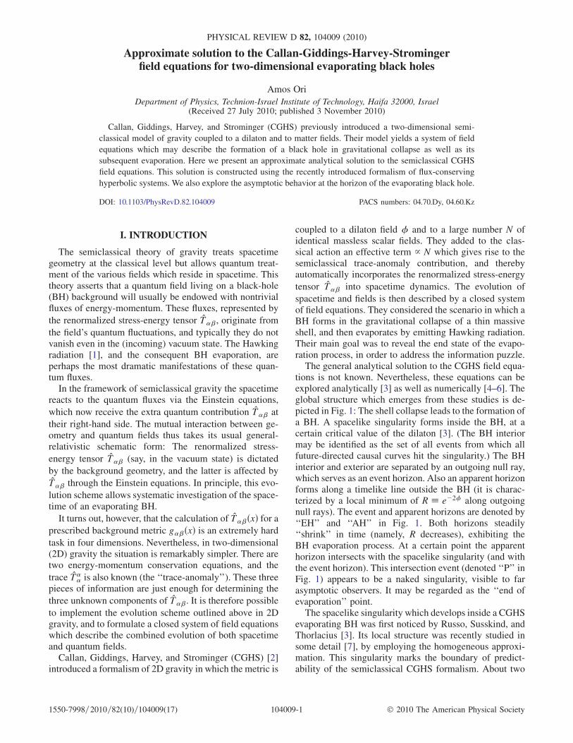


![Callan Teo Stage 02 Portuguese[1]](https://static.documents.pub/doc/80x56/55cf9de3550346d033afb5c7/callan-teo-stage-02-portuguese1.jpg)


