Approximate Voronoi Cell Computation on

Geometric Data Streams

Mehdi Sharifzadeh� and Cyrus Shahabi

Computer Science DepartmentUniversity of Southern California

Los Angeles, California 90089-0781[sharifza, shahabi]@usc.edu

Abstract. Several studies have exploited the properties of Voronoi di-agrams to improve variations of the nearest neighbor search on storeddatasets. However, the significance of Voronoi diagrams and their basicbuilding blocks, Voronoi cells, has been neglected when the geometry datais incrementally becoming available as a data stream. In this paper, westudy the problem of Voronoi cell computation for fixed 2-d site pointswhen the locations of the neighboring sites arrive as geometric data streams.We show that the non-streaming solution to the problem does not meetthe memory requirements of streaming applications over a sliding win-dow. Hence, we propose AVC and AVC-SW, two approximate streamingalgorithms that compute ε-approximations to the actual Voronoi cell inO(κ) using O(κ) space where κ is their sample size. With the sliding win-dow model, we prove both theoretically and experimentally that AVC-SWsignificantly reduces the average memory requirements of the classic al-gorithm, specially when the window size w is large, which is the case inreal-world scenarios.

1 Introduction

Different variations of the Voronoi diagrams have been theoretically studied in thefield of computational geometry. The Voronoi diagram of a set of points partitionthe space into a set of convex polygons so that each polygon contains exactly onepoint of the set. The polygon corresponding to each point p contains the pointsin the space that are closer to the point p than to any other point in the set. Thecomputational geometry literature refers to the polygons as Voronoi cells, Dirichletregions, Thiessen polytopes, or Voronoi polygons [5, 13].

In practice, different research areas in databases such as spatial databases,content-based image retrieval, and data mining have exploited the properties ofthe Voronoi diagrams to address variations of the nearest neighbor search in dif-ferent spaces [14]. The body of research in these areas is focused on improving theperformance of the nearest neighbor queries when the data tuples are stored asa massive dataset. However, the emerging trend of the data stream research ex-poses several fundamental challenges to this problem when the data in its entirety

� Contact author, phone: 1 (213) 740-2295, fax: 1 (213) 740-5807.

II

is not available to be processed. This radical change in the assumptions ariseswhen modern applications generate bulky fast-rate data streams. A large class ofthese applications continuously generate geometric data streams. Examples includeGPS equipments in today’s personal devices such as cell phones, PDAs, laptopsand cars that generate streams of geospatial data as well as more special-purposeapplications such as sensor networks [3] and immersive environments [15]1.

The adaption of the idea of Voronoi diagrams to various forms of the nearestneighbor search for geometric data streams requires reconsideration of the algo-rithmic aspects of building these data structures. Although a few research papershave been published recently to revisit classic computational geometry problemsin a data stream framework [6, 4, 10], to the best of our knowledge no study has re-considered the problem of building Voronoi diagrams or related data structures inthis framework. In this paper, we study the problem of computing Voronoi cells offixed points with respect to a sliding window over the data stream of 2-d site points.The cells can be used to solve different problems such as reverse nearest neigh-bor search [17]. As a real-world application, consider the sensor nodes in a sensornetwork deployed to monitor a physical phenomena such as soil temperature. Theaverage temperature of an area can be computed as the weighted average of thetemperature values recorded by each sensor node to provide a seamless average,independent of the density of the network. In this case, each node’s weight can bethe area of its Voronoi cell [16]. Each immobile node, knowing its fixed location,frequently receives the locations of other mobile/immobile nodes as a geometricdata stream and maintains its Voronoi cell with respect to these locations.

We show that with the general time series model [12], the classic algorithm forcomputing exact Voronoi cell of a point p simply drops any newly arrived pointwhich is not changing the cell. However, with the sliding window model, wherethe size of the window is w, the classic algorithm requires to store all the w points(i.e., O(w) space complexity) to continuously maintain the Voronoi cell given thew recent points. The reason is that even though an arriving point may not bechanging the cell at the time of the point’s arrival through the stream, it maycause a change in future due to the deletion of old points from the window. Tobe precise, with a fixed w, w insertions and w deletions occur during the lifetimeof a point inside the window. Any single deletion in the window may cause anypoint in the window to contribute to the cell while any insertion may end a point’scontribution (see the motivating example in Section 3).

Note that in real-world scenarios w is very large because its size is only limitedby the amount of available memory. A widely available 1GB of memory spacecan easily store w=100 million points of size 10 bytes each. From an applicationperspective, a time-based window of one day over 10 streams, with a rate of 100points/second per stream, contains the same number of points. To reduce the O(w)space complexity of the classic algorithm in sliding window model, we first proposeAVC, an approximation algorithm for the time series model which maintains onlya sample of the streamed points using the similar sampling technique describedfor building radial histograms in [4] and maintaining convex hull of data streams

1 See the related section in SQR: A Stream Query Repository, http://www-db.stanford.edu/stream/sqr/immersive.html.

III

in [10]. AVC employs the classic algorithm to build the Voronoi cell of the sampleas an approximation to the exact cell. The AVC’s time complexity of an updateper-point is O(κ) where κ is the sample size. The value of κ is determined based ona single parameter k that is independent of the distribution of the points. For thesliding window model, we propose an extension to AVC, AVC-SW, with the sametime and space complexities. However, the sample size of AVC-SW is dependenton both the parameter of the algorithm and the distribution of the points in thestream. We show that for a uniform site point distribution, the average size of thesample maintained by AVC-SW is far less than the window size w, specially forlarge w’s. Even though our simple experiments show 80% reduction in memoryusage by AVC-SW as compared to the classic algorithm (Section 7), we prove thatthis reduction is even more when w � k. For a uniform point distribution, wetheoretically compute the sample size of AVC-SW in terms of the window size andits single parameter. We show that the sample size grows very slowly as the ratio ofwindow size w over k increases. For instance, it is less than 20k for w/k ≤ 2.5×108.

Our main contribution resides in our analytical proofs and experimental results.We study the properties of our approximation algorithms (Section 5) and computetheir approximation error for a general nearest neighbor search through detailanalysis. More importantly, we theoretically prove that one can determine thesingle parameter of AVC (and AVC-SW) based on user’s tolerable error ε (Section6). We show that both AVCs compute an ε-approximation to the Voronoi cellin O(κ) per-point computation time and with O(κ) memory where κ is the sizeof their sample. Both AVCs can be incorporated within a general histogram-likesampling framework [4]. Moreover, the size of their approximate Voronoi cell isindependent from the complexity of the actual cell and the distributions of thepoints.

2 Definitions

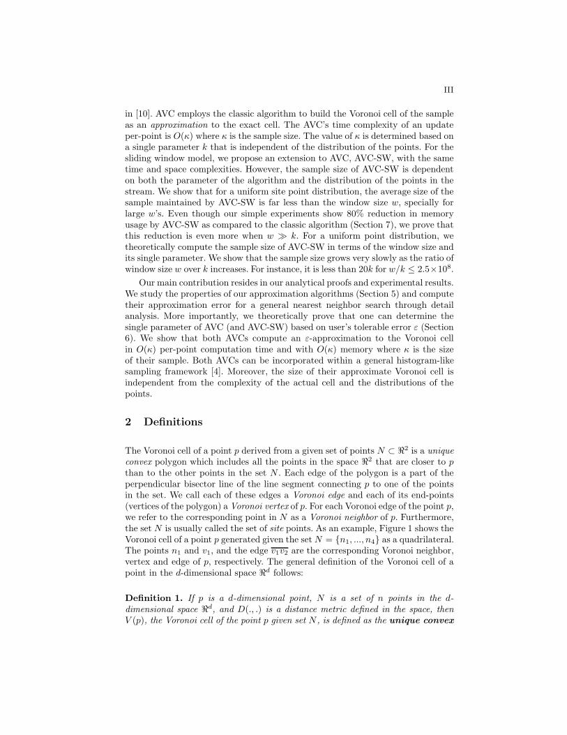
The Voronoi cell of a point p derived from a given set of points N ⊂ �2 is a uniqueconvex polygon which includes all the points in the space �2 that are closer to pthan to the other points in the set N . Each edge of the polygon is a part of theperpendicular bisector line of the line segment connecting p to one of the pointsin the set. We call each of these edges a Voronoi edge and each of its end-points(vertices of the polygon) a Voronoi vertex of p. For each Voronoi edge of the point p,we refer to the corresponding point in N as a Voronoi neighbor of p. Furthermore,the set N is usually called the set of site points. As an example, Figure 1 shows theVoronoi cell of a point p generated given the setN = {n1, ..., n4} as a quadrilateral.The points n1 and v1, and the edge v1v2 are the corresponding Voronoi neighbor,vertex and edge of p, respectively. The general definition of the Voronoi cell of apoint in the d-dimensional space �d follows:

Definition 1. If p is a d-dimensional point, N is a set of n points in the d-dimensional space �d, and D(., .) is a distance metric defined in the space, thenV (p), the Voronoi cell of the point p given set N , is defined as the unique convex

IV

n1

n2

x

n4

p

n3

V(p)

v1

v2

B(p,x)

H+(p,x)

H-(p,x)

Fig. 1. The Voronoi cell of the point p with respect to N = {n1, ..., n4}. The bisectorline corresponding to the new point x intersects with V (p) and excludes all the points inH−(p, x) from V (p).

polygon which contains all the points in the set Vn(p) 2:

Vn(p) = {q ∈ �d | ∀ n ∈ N,D(q, p) < D(q, n)}

Throughout this paper, we assume that the points are in 2-dimensional spaceand the distance metric is Euclidian. We use |pq|, pq, and B(p, q) to denote theEuclidian distance between the points p and q, the line segment connecting them,and the perpendicular bisector line of this segment, respectively. We use υ(p) torefer to the set of Voronoi neighbors of p. It is clear that the Voronoi cell V (p) canbe computed using υ(p) in O(1) time and vice versa. Hence, we use V (p) and υ(p)interchangeably throughout the paper.

3 The Problem

Assume that we need to compute V (p), the Voronoi cell of a given fixed point pwith respect to a set of n site points N . For each point q ∈ N , the line B(p, q)divides the space into two half-planes: H+(p, q) including p and H−(p, q) includingq. For any point in H−(p, q), we say that B(p, q) excludes the point from V (p) (seeFigure 1). The trivial way to find V (p) is to find the common intersection of all nhalf-planes H+(p, x) for all points x ∈ N . V (p) is the boundary of the intersection.If we use linear programming, the intersection is computed in O(n log n) time andlinear storage [5].

In this paper, we study two variations of the problem. First, consider the casewhen the points in N become incrementally available as a data stream. That is, ateach time instance t, only one point nt arrives, and we update N to N ∪{nt}. Thepoint p could be the fixed location of an immobile sensor node in the motivatingexample of Section 1. The node incrementally receives the locations of the othernodes (i.e., points in N) through a data stream. Here, the update scheme of Nis broadly referred as time series model in the data stream literature [12]. Nowthe problem is to update V (p) (or υ(p)) according to the updates to N (i.e, when

2 We assume that such a bounded polygon exists. Furthemore, we assume that p �∈ N .While this convention is different from the literature on Voronoi diagrams, the resultis the same.

V

p p p p

p p p p

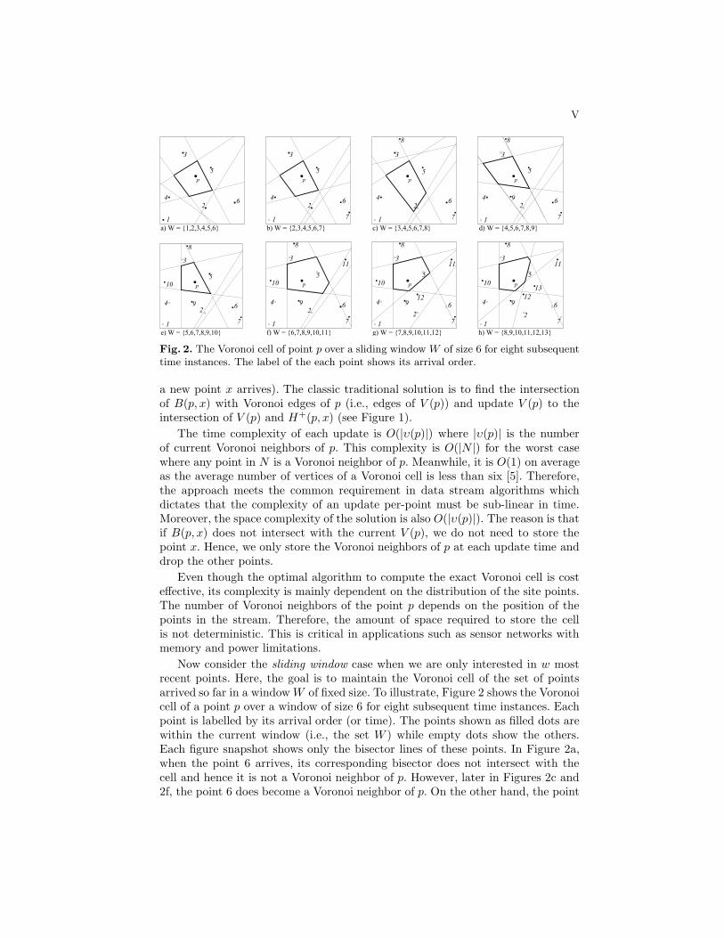
Fig. 2. The Voronoi cell of point p over a sliding window W of size 6 for eight subsequenttime instances. The label of the each point shows its arrival order.

a new point x arrives). The classic traditional solution is to find the intersectionof B(p, x) with Voronoi edges of p (i.e., edges of V (p)) and update V (p) to theintersection of V (p) and H+(p, x) (see Figure 1).

The time complexity of each update is O(|υ(p)|) where |υ(p)| is the numberof current Voronoi neighbors of p. This complexity is O(|N |) for the worst casewhere any point in N is a Voronoi neighbor of p. Meanwhile, it is O(1) on averageas the average number of vertices of a Voronoi cell is less than six [5]. Therefore,the approach meets the common requirement in data stream algorithms whichdictates that the complexity of an update per-point must be sub-linear in time.Moreover, the space complexity of the solution is also O(|υ(p)|). The reason is thatif B(p, x) does not intersect with the current V (p), we do not need to store thepoint x. Hence, we only store the Voronoi neighbors of p at each update time anddrop the other points.

Even though the optimal algorithm to compute the exact Voronoi cell is costeffective, its complexity is mainly dependent on the distribution of the site points.The number of Voronoi neighbors of the point p depends on the position of thepoints in the stream. Therefore, the amount of space required to store the cellis not deterministic. This is critical in applications such as sensor networks withmemory and power limitations.

Now consider the sliding window case when we are only interested in w mostrecent points. Here, the goal is to maintain the Voronoi cell of the set of pointsarrived so far in a windowW of fixed size. To illustrate, Figure 2 shows the Voronoicell of a point p over a window of size 6 for eight subsequent time instances. Eachpoint is labelled by its arrival order (or time). The points shown as filled dots arewithin the current window (i.e., the set W ) while empty dots show the others.Each figure snapshot shows only the bisector lines of these points. In Figure 2a,when the point 6 arrives, its corresponding bisector does not intersect with thecell and hence it is not a Voronoi neighbor of p. However, later in Figures 2c and2f, the point 6 does become a Voronoi neighbor of p. On the other hand, the point

VI

7 never become a Voronoi neighbor of p during any of the time instances whenthe point 7 is in the current window (Figures 2b-2g). This example shows thatthe traditional algorithm cannot drop a new point (e.g., point 6) even thoughits corresponding bisector does not intersect currently with the cell. That is, thespace complexity of the algorithm is O(|W |) where |W | is the size of the window3. Therefore, the traditional algorithm is not scalable as data stream rate andwindow size grow. Motivating by this observation, we first propose an algorithmto maintain an approximate Voronoi cell in the general time series model (Section4). In Section 7, we extend our algorithm to be applicable over a sliding window.

4 The Approximate Voronoi Cell Algorithm (AVC)

We want to maintain an approximation to the Voronoi cell of the point p whilethe site points in N are arriving as a data stream. The core idea behind our AVCalgorithm is to maintain a minimum subset of N including the closest site pointsto p and compute the Voronoi cell of p with respect to this subset instead of N .This cell is an approximation to the exact Voronoi cell given the entire N .

We divide the 2-d space using k vectors in k different directions. Each vectororiginates from the point p. Moreover, the angle between each pair of neighboringvectors is θ = 2π/k. We will show in Section 6 that the value of k can be determinedas a function of the user’s tolerance for error. As Figure 3a shows, the vectorspartition the space into k identical sectors. For each sector Si, we store a pointm(Si), the closest site point to the point p which is inside Si. We refer to thispoint as the minimum point of the sector Si. When a new point x arrives throughthe stream, first we find the sector Si containing x. Then, we replace the minimumpoint of the sector (m(Si)) with x if the point p is closer to the point x than tothe point m(Si).

Now the Voronoi cell of p derived from the set of k minimum points correspond-ing to k sectors (MN =

⋂1≤i≤k{m(Si)}) is an approximation of the actual Voronoi

cell of p using the set N . It is clear that the approximate Voronoi cell of p, containsits actual Voronoi cell. We can compute the approximation in O(k log k) time andspace at any time using the classic algorithm from the scratch. By incrementallyupdating this approximation on new point arrivals, the per-point computationcan be reduced to O(k). Furthermore, the time complexity of the per-point sam-ple update is also O(k) which can be improved to O(log k) using a searchable datastructure [10]. Hence, the per-point update time of AVC including the time for up-dating both the sample and the approximation is O(k). Therefore, AVC maintainsa sample of size κ = k to improve in terms of both time and space complexity overthe classic algorithm when k < |υ(p)|.

Throughout this paper, we use AVC(θ) to denote our algorithm with parameterθ in k = 2π/θ specifying the number of sectors. Furthermore, we use V ′(p) to referto AVC’s approximation to the Voronoi cell of the point p. Figure 3b shows theexact Voronoi cell of p with respect to the set N = {a, b, c, d, e, f, g, h}. Figure 3cshows V ′(p) created by AVC(θ = π/8). The filled dots in the figure are minimumpoints of the sectors while the empty dots are dropped by AVC.3 In fact, deciding to drop a new point is significantly expensive for the traditional

algorithm (i.e., O(|W |2)). Details are removed due to the lack of space.

VII

p

θ

a

b c

e

g

b

f

d

a

b c

e

g

b

f

d

Fig. 3. a) k = 16 vectors originating from p divide the space into k identical sectors, b)The Voronoi cell of the point p, and c) The approximate Voronoi cell of p.

5 Properties of AVCIn this section, we study different properties of the approximate Voronoi cell com-puted by the AVC algorithm. We use these properties to compute the approxima-tion error of the algorithm in terms of the parameter θ.

A primary property of the Voronoi cell of a point p is that it contains none ofthe site points4. We intend to maintain this property for the approximate Voronoicell. It is trivial that the output of AVC(θ) depends on both the value of θ andthe distribution of the site points in N . However, we show that specific values of θcan be used in AVC to make some properties of its output independent from thedistribution of the input points.

Lemma 1. For any point p, V ′(p) computed by AVC(θ) does not contain any ofthe site points in N for any arbitrary set N if and only if θ is less than π/3.

Proof. See Appendix A.

Another property of the Voronoi cell of p is that the distance of any pointinside (on) the cell to p is less than (equal to) its distance to any site point in N .We show that for any point inside (on) the approximate Voronoi cell of a point p,its distance to its closest site point in N is less than its distance to p by at mosta small factor. We define the function f(q) over the set of points q in 2-d space as

f(q) =|qp||qr| (1)

where r is the closest site point to q in N . The property indicates that f(q) isalways less than or equal to 1 for the set of points inside or on V (p). Over this set,the function f reaches its upper bound (one) on the points on the boundary ofV (p). To study the approximation error of the AVC algorithm, we need to find theupper bound of the function over the set of points inside or on V ′(p). In particular,if a point is inside or on V ′(p) we find how far its distance to p from its distanceto its actual closest point could be. Towards this end, we first locate the pointswhere the maximum of f(q) occurs.4 Note that p �∈ N .

VIII

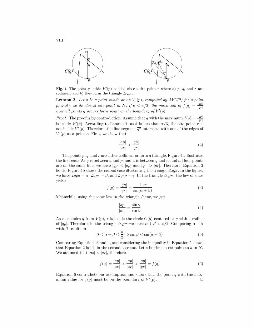
Fig. 4. The point q inside V ′(p) and its closest site point r where a) p, q, and r arecollinear, and b) they form the triangle �qpr.

Lemma 2. Let q be a point inside or on V ′(p), computed by AVC(θ) for a pointp, and r be its closest site point in N . If θ < π/3, the maximum of f(q) = |qp|

|qr|over all points q occurs for a point on the boundary of V ′(p).

Proof. The proof is by contradiction. Assume that q with the maximum f(q) = |qp||qr|

is inside V ′(p). According to Lemma 1, as θ is less than π/3, the site point r isnot inside V ′(p). Therefore, the line segment qr intersects with one of the edges ofV ′(p) at a point a. First, we show that

|ap||ar| >

|qp||qr| . (2)

The points p, q, and r are either collinear or form a triangle. Figure 4a illustratesthe first case. As q is between a and p, and a is between q and r, and all four pointsare on the same line, we have |qp| < |ap| and |qr| > |ar|. Therefore, Equation 2holds. Figure 4b shows the second case illustrating the triangle �qpr. In the figure,we have � qpa = α, � apr = β, and � qrp = γ. In the triangle �qpr, the law of sinesyields

f(q) =|qp||qr| =

sin γsin(α+ β)

(3)

Meanwhile, using the same law in the triangle �apr, we get

|ap||ar| =

sin γsinβ

(4)

As r excludes q from V (p), r is inside the circle C(q) centered at q with a radiusof |qp|. Therefore, in the triangle �qpr we have α + β < π/2. Comparing α + βwith β results in

β < α+ β <π

2⇒ sinβ < sin(α+ β) (5)

Comparing Equations 3 and 4, and considering the inequality in Equation 5 showsthat Equation 2 holds in the second case too. Let s be the closest point to a in N .We assumed that |as| < |ar|, therefore

f(a) =|ap||as| >

|ap||ar| >

|qp||qr| = f(q) (6)

Equation 6 contradicts our assumption and shows that the point q with the max-imum value for f(q) must be on the boundary of V ′(p). �

IX

6 Approximation Error

We prove that the Voronoi cell computed by the AVC algorithm is an ε-approximationto the actual Voronoi cell. More precisely, if a point q is inside the approximateVoronoi cell of a point p, its distance to its closest point in N is less than itsdistance to p by at most a factor of 1 + ε (i.e., f(q) ≤ 1 + ε). We show that thisdifference is bounded and find the upper bound of ε for a given θ. Moreover, weprove that for a given ε, one can compute the largest θ for which AVC(θ) resultsin an approximation of tolerable error ε. To provide a proof, we first showed inLemma 1 that the maximum of the function f occurs on the edges of the approx-imate Voronoi cell. In this section, for an arbitrary point q on the approximateVoronoi cell of p but outside its actual Voronoi cell, we consider the set of its pos-sible closest points in N which might have been dropped by the AVC algorithm.We find the maximum of f(q) over the set of all points such as q.

Theorem 1. If q is a point on the boundary of V ′(p) computed by the algorithmAVC(θ) and r is its closest site point in N , a certain ε can be found in terms ofθ which

f(q) =|qp||qr| ≤ 1 + ε (7)

Proof. Let q be a point on one of the edges of the approximate Voronoi cell of pand outside the actual Voronoi cell of p (i.e., inside H−(p, r)). That is, the closestpoint to q in N ∪ {p} is a point r other than p. The goal is to find the maximumof |qp|/|qr|. Towards this objective, we need to find the minimum of |qr| as |qp| isfixed for q. Hence, we locate the closest such a point r to q. It is clear that thispoint is not among k minimum points corresponding to the sectors (i.e., r �∈MN).The reason is that if it was one of these points, the bisector line corresponding topr, B(p, r), would have excluded q from the approximate Voronoi cell of p in theAVC algorithm. However, an exact Voronoi cell computation algorithm causes qto be outside V (p). The locus of the points such as r which their correspondingbisector lines, B(p, r), exclude the point q from V (p) is inside a circle centered atq with a radius of |pq|. We call this circle C(q). To illustrate, consider the Voronoicell of point p showed in Figure 5a. The figure shows a point q inside the Voronoicell of p and the points x and y inside and outside the circle C(q), respectively.The bisector line B(p, x) intersects with the Voronoi cell causing q to be excludedfrom the cell. This is while, y which is outside the circle C(q) has no effect on theinclusion of q in the cell.

Now consider all the sectors which intersect with the circle C(q), namelyS1, ..., S9 in Figure 5b. As q is on V ′(p) we can infer that for each of these sectorseither it includes none of the points in N or its corresponding minimum point isoutside the circle C(q). However, because q is outside V (p) the former case cannotbe true for all of such sectors. That is, there must be at least one sector containingr with a minimum point outside the circle C(q). This minimum point has causedthe point r to be removed from our set of minimum points. Therefore, its corre-sponding bisector line has not excluded q from V ′(p) in the AVC algorithm. Tofind the minimum value of |qr|, we show how this happens and find the closestpoint r which has been removed because of this minimum point.

X

q

px

y

C(q)p

q

s

mS2

S3

S4

S1

S5

S9

S6

S7

S8

v1

O

Fig. 5. a) The effect of the two points x and y on the inclusion of q in the Voronoi cellof p. b) The point q on one of the edges of V ′(p), the intersection of the sectors with thecircle C(q), the hidden point of the sector S3, the angle β based on the location of q inS5, and the angle α based on the location of S3 and S5.

Consider one of the sectors that intersect with C(q) (S3 in Figure 5b). Let uslocate the intersection point of the boundaries of the sector and the circumferenceof C(q) which is closer to p (m in Figure 5b). The point m is the closest possibleminimum point to p inside S3 and outside C(q). Each of the points inside thesector and the circle C(q) whose distance to p is more than |mp| has been removedbecause of m. The locus of these points is the intersection of 1) inside the sectorS3, 2) inside the circle C(q), and 3) outside the circle centered at p with a radiusof |mp| (C). Figure 5b marks this intersection as O. The closest point to q in Ois the point s. We refer to s as the hidden point of the sector S3 with respect to qand V ′(p).

Now consider the hidden point of S3. Let v1 be the closest vector to q betweenpq and ps. We use α and β to refer to the angles which ps and pq make with v1,respectively (see Figure 5b). Notice that the location of q determines the value ofβ while α depends on the location of S3 with reference to the sector containing q(i.e., S5). Using the law of cosines in the triangle �pqs we have

|qs|2 = |qp|2 + |ps|2 − 2 · |qp| · |ps| · cos(α+ β) (8)

We have |ps| = |pm| as both s and m reside on the circle C. Moreover, the triangle�pqm is an isosceles triangle as both points p and m are on the circle C(q)(|qm| = |qp|). The angle between pm and ps is equal to θ as they are boundariesof the same sector. Now in the triangle �pqm we have |pm| = 2·|qp|·cos(α+β+θ).If we replace |ps| with the value of |pm| in Equation 8, we get

|qs|2 = |qp|2 + 4 · |qp|2 · cos2(α+ β + θ) − 4 · |qp|2 · cos(α + β) · cos(α+ β + θ)(9)

XI

We define F (α, β, θ) as

F (α, β, θ) =√

1 + 4 · cos2(α+ β + θ) − 4 · cos(α+ β) · cos(α+ β + θ) (10)

and replace it in Equation 9 to get

|qs| = |qp| · F (α+ β + θ) (11)

As r is the closest point to q, the point q is closer to the hidden point of thesector containing r (i.e., s inside S3 in Figure 5b) than to the hidden points ofall of the sectors that intersect with the circle C(q). To be precise, for a givenpoint q (with a fixed angle β) the value of |qs| in the sector containing r must beminimum over all other sectors (with different values of α) that intersect with thecircle C(q). To exploit the domain of the angle α, observe that as both points mand p are on the circle C(q), the angle � qpm = α+ β + θ is not greater than π/2.Therefore we have

|qs| = min0 ≤ α ≤ π

2 − β − θα = iθ

(|qp| · F (α+ β + θ)) (12)

We replace the value of |qs| in f(q) = |qp|/|qs| to obtain

|qp||qs| =

1minα = iθ F (α+ β + θ)

(13)

Now as |qr| ≥ |qs| for the sector containing r, we have

f(q) =|qp||qr| ≤

|qp||qs| (14)

Therefore, the upper bound of f(q) is not greater than the upper bound of |qp|/|qs|.The latter is the maximum of Equation 13 over different points q (with differentβ angles). Hence, for any point such as q

f(q) ≤ max0 ≤ β ≤ θ

(1

minα = iθ F (α+ β + θ)) (15)

Equation 15 shows an upper bound for f(q) as a function of α, β, and θ. In theremainder of the proof, we show that this function is bounded by another functionin terms of θ. Let α0 = argmin(|qs|). Figure 6a plots α0/θ for different valuesof k = 2π/θ and β, and Figure 6b shows a slice of this diagram for k = 36. Asshown in both figures, the value of α0 that determines the location of the points depends on both θ and β. It means that if q (and β) changes in Figure 5b,the sector containing r might change to be S4 (not S3). In general, for a given θthe polar angle between the sector containing a point inside V ′(p) and its closestpossible point which can be removed by AVC is not fixed.

Figure 6c plots the maximum of f(q) for different values of θ. As the figureshows, f(q) is less than 2 if k is greater than 16 (i.e., θ < π/8). For any value of θ,

XII

/2k

0

0.02 0.04 0.06 0.08 0.1 0.12 0.14 0.160

1

2

3

4

5

6

7

0

50 100 150 2001

1.5

2

2.5

3

3.5

4

4.5

5

max(f(q))g(theta)

/2k

))(max( qf

)(g

Fig. 6. a) α0/θ shows the location of the sector containing the closest hidden point to qfor different values of β and k (β is in radians), b) α0/θ for different values of β wherek = 36 (i.e., θ = π/18), c) The upper bound of f(q) for different values of k.

one can extract a certain ε = max(f(q))−1 from the Figure 6c so that Equation 7holds. To find a maximum function in terms of θ we plotted the following functionin this diagram:

g(θ) =1√

3 − 2√

2 · cos(π/4 − θ)(16)

The figure shows that for the values of k > 24, g(θ = 2π/k) is always greaterthan but very close to f(q). Consequently, the approximation error of AVC(θ) isbounded by g(θ). It implies that Equation 7 holds for ε = g(θ) − 1. �

The immediate implication of the proof of Theorem 1 is that for a given ε, wecan use g(θ) to compute the smallest k (i.e., the largest θ) to use with the AVCalgorithm and result in an approximation of tolerable error ε.

Theorem 2. For a given error bound ε, the largest θ, using which AVC(θ) cancompute an approximate Voronoi cell with a maximum error of ε is computed fromthe equation g(θ) = 1 + ε.

7 AVC over Sliding WindowsIn this section, we extend the AVC algorithm to be applicable to the sliding windowmodel. With this model, the goal is to maintain the Voronoi cell of a point p withrespect to the set of w recent points. With a window of fixed size w, when the newpoint nt is arrived through the data stream, we update the set of site points N toexclude its oldest point and include nt. We say the oldest point has been expired.

In Section 2, we showed that a traditional Voronoi cell computation algorithmcannot be used over a sliding window. The algorithm is not scalable to data streamrate and window size as it costs O(w) memory. Likewise, the AVC algorithm isprone to the same problems. As an example, assume that AVC stores the minimumpoint m corresponding to the sector S at time t. Assume that according to thewindow size, m expires at time t′ > t (i.e., when we receive w points after t).Consider the set of site points that arrive during the time range (t, t′) and residein the sector S. If p is closer to m than to any of these points, AVC drops all ofthem and maintains m as the minimum point of S. However, as soon as m expires,the minimum point of S needs to be updated to the point m′, the closest point to

XIII

1

p

S

a)

M(S) = {1}

m(S) = 1

1

p

S

b)

M(S) = {1,2}

m(S) = 1

2 1

p

S

c)

M(S) = {1,2,3}

m(S) = 1

2

3

1

p

S

d)

M(S) = {1,4}

m(S) = 1

2

3

4

1

p

S

e)

M(S) = {5}

m(S) = 5

2

3

4

5

Fig. 7. AVC-SW updates the set M(S) and the minimum point m(S) for each of the5 arriving points in the sector S. Assume that none of these points expire during thisillustration.

p in NS . Hence, AVC must store m′. Applying the reasoning recursively rendersthat AVC must store all the points in the window. In the remainder of this section,we extend the AVC algorithm to overcome this shortcoming by storing only thepoints which might become a minimum point in a future window.

With the AVC algorithm, we require to maintain the minimum points of eachsector for the current window. The main idea behind our extension (AVC-SW)is that for each sector, any point arrived earlier than the sector’s current closestpoint to p could not be minimum in any of the future windows. Therefore, we candrop this point. Otherwise, we store it as it might be the minimum point in afuture window before it expires.

7.1 The AVC-SW AlgorithmLet w be the window size, and at each time instance t, only one point arrives. Weemploy the same vectors of AVC to divide the space into sectors (see Section 4).For each sector Si, we store the minimum point m(Si) and a set of points M(Si).This set includes all the points which are likely to be minimum points in the futurewindows. We initialize m(Si) and M(Si) to null for all sectors Si before we startprocessing the data stream.

For each new point x, first we find the expired point among members of allM(Si) sets and delete it. Second, we find the sector S containing x and add xto M(S). Third, we delete any point y in M(S) if |py| > |px|. These points willnever become minimum point of their sector in a future window. Finally, we setm(S) to the closest point to p in M(S). Similar to AVC, the Voronoi cell of pderived from the set of k minimum points (m(Si)) corresponding to k sectors isthe approximation of the actual Voronoi cell of p. The properties of V ′(p) and theapproximation error analysis discussed in Sections 5 and 6 also hold for the outputof AVC-SW. The sample size of AVC-SW is computed as κ =

∑ki=1 |M(Si)|, where

|M(Si)| is the cardinality of the set M(Si).Figure 7 illustrates how AVC-SW maintains the minimum points of the sector

S. The figure shows only the times when the new point is inside the sector S.Assume that none of these points expires during these time instances. As shownin Figure 7a, the point 1 is the current minimum point of S. When the point 2and 3 arrive in Figures 7b and 7c, respectively, AVC-SW adds them to M(S) asthey might become the minimum point of S when 1 expires. However, 1 is still the

XIV

0

80

160

240

320

400

480

7 17 27 37 47 57 67 77 87 97AVC-SW's Parameter (k)

AV

C-S

W's

Sam

ple

Siz

e

w = 80 w = 240 w = 400

0

100

200

300

400

500

600

700

800

1 51 101 151 201 251 301 351 401 451 501 551 601 651 701 751

Window Size (w)

Window Size

AVC-SW's Sample Size

Fig. 8. a) Average number of points stored by AVC-SW (i.e., AVC-SW’s sample size)for a) w = 80, 240, and 400 and different values of k, and b) different values of w whenk = 36.

current minimum point of S in the window. In Figure 7d, the point 4 arrives. As4 is in all future windows in which 2 or 3 exist and p is closer to 4 than to 2 and 3,we delete 2 and 3. Finally, the point 5 arrives in Figure 7e and causes the updateto the minimum point and deletion of all the points in M(S).

In general case, the space requirements of AVC-SW is less than O(w) as wedrop the portion of the points that are unlikely to be a minimum point. However,in the worst case, when the points of each sector arrive in the increasing order oftheir distance to p, AVC-SW stores all of them (see Figures 7a-7c). We conductedan experiment to evaluate the average space used by AVC-SW. We syntheticallygenerated data streams of 1000 points uniformly distributed inside a circle. Weapplied AVC-SW’s sampling algorithm on the stream and computed the averagenumber of stored points during 100 runs. Figure 8a illustrates the sample size (κ)of AVC-SW for different values of k when we vary the window size. It shows thatfor window sizes greater than k, the sample size is far less than w. Figure 8b showsup to 80% reduction in memory requirement for k = 36 and large windows.

7.2 Space Requirements Analysis

In this section, we theoretically find the average number of the points stored byAVC-SW. Let w and k be the window size and the number of sectors used by AVC-SW, respectively. For a uniform distribution of the points in the space, each sectorincludes w/k points. For now, we assume that n = w/k is an integer. Assumethat on average, AVC-SW stores A(i) points of i points contained in each sector.In other words, A(i) is the average size of the set M(Sj) for the sector Sj . Wecompute A(n), the average number of points in a window of size w which AVC-SWstores corresponding to each sector. Hence, the total number of points stored byAVC-SW will be κ = k.A(n).

AVC-SW uses the order of the points received in each sector and their distanceto the center point p to decide whether they must be stored or dropped. For a sectorS, assume that i points of the current window are inside S. We show these pointsas an i-tuple P = (p1, p2, . . . , pi). The point pj is the j-th arrived point whichis inside the sector S. We sort these points based on their increasing distance tothe point p and rank them accordingly. To break the ties, for two points with the

XV

a

p

S

b

c

d

e

i = 5

P = (a, b, c, d, e)

R = (2, 4, 5, 3, 1)

M(S) = {e}

N(R) = 1

Fig. 9. .

same distance to p, we insert the point with greater polar angle with the x-axisafter the one with the smaller angle. The i-tuple R = (R1, R2, . . . , Ri) includesthe ranks in which 1 ≤ Rj ≤ i is the rank of the point pj in P . As P includesno redundant point, R is clearly a permutation of positive integers less than orequal i. Depending on the order of the points in the i-tuple P and their distanceto the center point p, R could be any of i! permutations of these numbers. Assumethat for the sector S including the points in P ranked as R, AVC-SW stores N(R)points. To illustrate, Figure 9 shows the sector S including five points a, b, c, d,and e. The order of their arrival time is given as the 5-tuple P with a and e as theoldest and the most recent points, respectively. R shows their ranks consideringtheir distances to p. AVC-SW stores only the point e so the value of N(R) is one.

Let Ti be the set of all permutations of positive integers less than i+ 1. More-over, let S(i) be the sum of values of N(R) for all permutations R ∈ Ti. In otherwords,

S(i) =∑

R∈Ti

N(R) (17)

Therefore, out of i points inside each sector, the average number of pointsstored by AVC-SW will be

A(i) =S(i)i!

(18)

It is clear that A(1) = S(1) = 1. We try to find S(i) and A(i) in terms of S(i−1)and A(i − 1), respectively. First, notice how Ti is generated using the membersof Ti−1. Inserting i before each number of a permutation in Ti−1 or after its lastnumber generates a unique permutation in Ti. For example, for the permutation(2, 1) in T2 = {(1, 2), (2, 1)}, we can generate permutations (3, 2, 1), (2, 3, 1), and(2, 1, 3) of T3 by inserting 3 before 2, before 1 and after 1, respectively. In general,we generate i members of Ti from each permutation in Ti−1. We use ΓR,i to referto the set of all permutations generated from R by the above approach. The abovegeneration scheme dictates that ΓR,i ∩ ΓR′,i = ø where R,R′ ∈ Ti−1 and R �= R′.Furthermore, obviously we have Ti =

⋃R∈Ti−1

ΓR,i.

XVI

Now, we determine the value of N(R′) for each permutation R′ ∈ Ti generatedfrom a permutation R ∈ Ti−1 (i.e., R′ ∈ ΓR,i). Given R = (R1, R2, . . . , Ri−1),R′ is generated by inserting i either before an Rj in R or exactly after Ri−1.In the first case, when we insert i before Rj to generate R′, it means that thecorresponding point q with rank i has arrived before the jth point (i.e., pj). AllRk’s in R are less than i. Recall that each Rj shows how close the jth arrivedpoint of a sector is to the center point p; the smaller Rj the closer pj to p. Hence,as we have Rj < i, the arrival of pj causes deletion of the point q by AVC-SW.It means that in the first case adding q (i.e., adding i to R) does not change thenumber of points stored by AVC-SW (i.e., N(R′) = N(R)). In the second case,when R′ is (R1, R2, . . . , Ri−1, i), AVC-SW stores the point q with the rank i as itmight become the minimum point of the sector in future windows. Subsequently,we have N(R′) = N(R) + 1. Therefore, we get

∑R′∈ΓR,i

N(R′) = i.N(R) + 1 (19)

Using Equation 17 we have

S(i) =∑

R∈TiN(R)

=∑

R∈Ti−1

∑R′∈ΓR,i

N(R′)= i.

∑R∈Ti−1

N(R) +∑

R∈Ti−11

= i.S(i− 1) + (i− 1)!

(20)

Dividing both sides of this equation by i! and considering the definition of A(i)given in Equation 18, we get the following for i > 1:

A(i) = A(i− 1) +1i

(21)

As we have A(1) = 1, rewriting Equation 21 yields

A(i) =i∑

j=1

1i

(22)

The above is the partial sum of the first i terms of the harmonic series. The sumA(i) is given analytically by the ith harmonic number Hi:

Hi = γ + ψ0(i+ 1) (23)

where γ is the Euler-Mascheroni constant and ψ0(x) is the digamma function.Although the series diverges when i increases, Hn has proven to be increasingslowly. For i ≤ 2.5 × 108 terms, it is still less than 20. Furthermore, to get Hn

greater than 100, 1.509× 1043 terms of the series is needed [7].So far, we have computed the average number of points of each sector stored

by AVC-SW. Therefore, if the number of points in each sector n = w/k is aninteger, AVC-SW stores only κ = k.Hn points out of w points. If w/k is notan integer, we set n = �w/k� and m = w mod k. For a uniform distributionof points in a window of size w, k − m sectors include n points and m sectors

XVII

0

100

200

300

400

500

600

700

800

7 72 144 216 288 360 432 504 576 648 720 792

Window Size (w)

Window Size

AVC-SW's Analytical Sample Size

Fig. 10. Analytical average number of points stored by AVC-SW (i.e., AVC-SW’s samplesize κ) for different values of w when k = 36.

include n+ 1 points. Therefore, the sample size of AVC-SW for window size w isκ = (k −m).Hn +m.Hn+1. As we have Hn+1 = Hn + 1/(n+ 1), we simplify κ toget the following for the general case:

κ = k.Hn +m

n+ 1(24)

Considering the above equation, the sample size κ is less than 20k when w ≤2.5 × 108 × k. Figure 10 shows the value of κ computed using Equation 24 fork = 36 sectors and different window sizes. Notice that the number of sectors is thesame as that of results shown in Figure 8b. Comparing two figures proves that theanalytical sample size computed as Equation 24 completely supports the samplesize computed during our experimental results.

8 Related Work

The field of computational geometry (CG) is a rich area of investigation for thedata stream algorithms [12]. Recently, a few studies have been focused on CGproblems on data streams. In [6], Feigenbaum et al. find the diameter and con-vex hull of a geometric data stream over a sliding window. Their sample uses O(r)space with O(r) andO(log r) processing time per point to maintain a (1+O(1/r2))-approximation and (1+O(1/r))-approximation, respectively. In [4], Cormode et al.use the same sampling method as AVCs to build radial histograms and approx-imate a number of geometric aggregates such as diameter and furthest neighborsearch on 2-d point data streams. In [10], Hershberger et al. introduce adaptivesampling to maintain an approximate convex hull of geometric data streams witha distance of O(D/r2) from their accurate convex hull, where D is the diameter oftheir sample set. To the best of our knowledge, no study have considered buildingVoronoi-related data structures on geometric data streams.

Different variations of Voronoi diagrams have been used as index structures forthe nearest neighbor search. In [8], Hagedoorn introduces a directed acyclic graphbased on Voronoi diagrams. He uses the data structure to answer exact nearest-neighbor queries with respect to general distance functions in O(log2 n) time usingonly O(n) space. Stanoi et al. in [17] combine the properties of Voronoi cells(influence sets in their terminology) with the efficiency of R-trees to retrieve reversenearest neighbors of a query point from the database. As a more practical example,

XVIII

Kolahdouzan et al. [11] propose a Voronoi-based data structure to improve theperformance of exact k-nearest neighbor search in spatial network databases.

Arya et al. [1] focus on approximating the Voronoi diagrams globally to an-swer ε-nearest neighbor queries. They build cells with the shape of hypercubesor the difference of two hypercubes. Har-Peled [9] partitions the space with anapproximation of Voronoi diagrams. His space decomposition generates a com-pressed quadtree of size O(n log n

εd log nε ) that answers ε-nearest neighbor queries

in O(log(n/ε)) time. Arya et al. [2] have performed the only work on approxi-mating Voronoi cells in d-dimensional space. Their approach combines the shapeapproximation and adaptive sampling techniques to build an approximate cell ofsize O(1/

√ε) for d=2. They assume that the accurate cell to be approximated is

given. Then, they examine the Voronoi neighbors of the given point and the cor-responding Voronoi vertices to keep the minimum number of Voronoi neighborsusing which an ε-approximate cell for addressing nearest neighbor problem can becomputed. This approach is not applicable to sliding windows over data streamsas insertion/deletion of each single point might cause the sampling criteria to in-clude or exclude a neighbor from the cell. This non-deterministic change resultsinto storing all the points in the window.

9 Conclusion

We proposed AVC and AVC-SW algorithms for approximating a Voronoi cell ongeometric point streams in time series and sliding window models, respectively.We theoretically computed the approximation error of our algorithms in terms oftheir single parameter. Our main findings are as follows:– AVCs result ε-approximations to the Voronoi cell.– Using Theorem 2, the parameter k (or θ) of AVCs can be computed based on

the user’s tolerable error.– With the sliding window model, AVC-SW significantly improves the space

complexity of the classic algorithm when the window size is greater than itsparameter k.

References

1. S. Arya, T. Malamatos, and D. M. Mount. Space-efficient approximate voronoidiagrams. In Proceedings of the 34th ACM Symp. on Theory of Computing (STOC),pages 721–730, 2002.

2. S. Arya and A. Vigneron. Approximating a voronoi cell. Technical report, 2003.HKUST-TCSC-2003-10.

3. P. Bonnet, J. E. Gehrke, and P. Seshadri. Towards Sensor Database Systems. InProceedings of the Second International Conference on Mobile Data Management,pages 3–14, 2001.

4. G. Cormode and S. Muthukrishnan. Radial histograms for spatial streams. DIMACSTR 2003-11, 2003.

5. M. de Berg, M. van Kreveld, M. Overmars, and O. Schwarzkopf. ComputationalGeometry: Algorithms and Applications. Springer Verlag, 2nd edition, 2000.

6. J. Feigenbaum, S. Kannan, and J. Zhang. Computing diameter in the streaming andsliding-window models, 2002. Manuscript.

7. M. Gardner. The Sixth Book of Mathematical Games from Scientific American.University of Chicago Press, 1984.

XIX

8. M. Hagedoorn. Nearest neighbors can be found efficiently if the dimension is smallrelative to the input size. In Proceedings of the 9th International Conference onDatabase Theory - ICDT 2003, volume 2572 of Lecture Notes in Computer Science,pages 440–454. Springer, January 2003.

9. S. Har-Peled. A replacement for voronoi diagrams of near linear size. In Proc. 42ndAnnu. IEEE Sympos. Found. Comput. Sci., pages 94–103, 2001.

10. J. Hershberger and S. Suri. Adaptive sampling for geometric problems over datastreams. In Proceedings of the Twenty-third ACM SIGACT-SIGMOD-SIGART Sym-posium on Principles of Database Systems. ACM, 2004.

11. M. R. Kolahdouzan and C. Shahabi. Voronoi-based k nearest neighbor search forspatial network databases. In Proceedings of the 30th International Conference onVery Large Data Bases (VLDB’04), 2004.

12. S. Muthukrishnan. Data streams: Algorithms and applications. Technical report,Computer Science Department, Rutgers University, 2003.

13. A. Okabe, B. Boots, K. Sugihara, and S. N. Chiu. Spatial Tessellations, Conceptsand Applications of Voronoi Diagrams. John Wiley and Sons Ltd., 2nd edition, 2000.

14. H. Samet. Applications of Spatial Data Structures: Computer Graphics, Image Pro-cessing, and GIS. Addison-Wesley, 1990.

15. C. Shahabi. AIMS: An immersidata management system. In Proceedings of the firstConference on Innovative Data Systems Research (CIDR’03), January 2003.

16. M. Sharifzadeh and C. Shahabi. Supporting spatial aggregation in sensor networkdatabases. In Proceedings of the 12th ACM International Symposium on Advancesin Geographic Information Systems - ACM GIS’04, 2004. To Appear.

17. I. Stanoi, M. Riedewald, D. Agrawal, and A. E. Abbadi. Discovery of Influence Sets inFrequently Updated Databases. In Proceedings of the 27th International Conferenceon Very Large Data Bases (VLDB’01), pages 99–108. Morgan Kaufmann PublishersInc., 2001.

XX

Appendix

A The Proof of Lemma 1Proof. First, assume that θ < π/3 and the point q ∈ N is inside V ′(p). The proofis by contradiction. Let S be the sector containing q. It is clear that q cannotbe the minimum point of S as V ′(p) is the Voronoi cell of p with respect to theminimum points in N . Hence, suppose m is the minimum point corresponding toS (i.e., m = m(S)) as shown in Figure 11a. Therefore, we have |pq| > |pm|. As qand m are both inside the same sector S, the angle between pm and pq, α = � qpm,is less than θ. Therefore, α < π/3. In the triangle �pqm, |pq| > |pm| concludesthat γ > β. Moreover, as α, β, and γ are the angles of the same triangle, thusα + β + γ = π. At least one of the angles β or γ must be greater than π/3 asα < π/3. The fact that γ > β yields that γ > π/3 > α. That is, in the triangle�pqm, we have |pq| > |mq| and hence, q is closer to m than p. Therefore, thebisector of pm, B(p,m), would exclude q from V ′(p). This means that V ′(p) doesnot contain the point q which contradicts our assumption.

m

p

q

Sm

p

S

B(p,m)n

l2

l1

C

H (p,m)+

H (p,m)_

O

Fig. 11. The sector S and its minimum point m where a) θ < π/3, and b) θ > π/3

Now assume that the angle θ is greater than π/3. We show that there exist aset of potential points in N which are not excluded from V ′(p) by any of bisectorlines corresponding to the minimum points. Figure 11b shows a sector S and itsboundaries l1 and l2. Assume that the corresponding minimum point of S, m, is onl1. The locus of all the points in the sector S which are removed from N becauseof the minimum point m is outside the circle C centered at p with a radius of |pm|.The bisector line B(p,m) intersects with the circle C at point n. We show thatthis point is inside S. As n is on B(p,m) we have |mn| = |pn|. Besides, as n ison the circle C, thus |pn| = |pm|. Therefore, the triangle �pmn is an equilateraltriangle. Hence, the angle α = � mpn = π/3. This yields that α < θ. Therefore,the point n is inside the sector S. Now consider the intersection of the sector S,outside of the circle C, and H+(p,m) (marked as O in Figure 11b). As n is insideS, this intersection is not empty. The AVC algorithm removes any point in thisintersection because of the minimum point m. However, the bisector line B(m, p)does not exclude these points from the approximate Voronoi cell of p. For anypoint q in this area, if none of bisector lines corresponding to the minimum pointsof other sectors excludes q from V ′(p), q will be inside V ′(p).5 �5 When θ = π/3, n is the only point in O which reside on the edge of V ′(p) if no other

bisector line excludes it from V ′(p).