Approximation and visualization of Pareto frontier:

Interactive Decision Maps technique

Alexander V. Lotov

Dorodnicyn Computing Centre of Russian Academy of Sciences, and

Lomonosov Moscow State University, Russia

Part 1

Plan of the talk

1. Few words concerning multi-objective optimization 2. Pareto frontier methods 3. Visualization: why it is needed?4. Interactive Decision Maps (IDM) technique for visualization of Pareto frontier: software demo5. Mathematics of the IDM technique in convex case6. Real-life applications of the IDM 7. IDM in Web Participatory Decision Support8. IDM in the non-convex case9. Current studies

Detailed information on the IDM technique is given in the book

Lotov A.V., Bushenkov V.A., and Kamenev G.K.

Interactive Decision Maps. Approximation and Visualization

of Pareto Frontier. Kluwer Academic Publishers, 2004.

Notation

Z=f(X) = feasible set in criterion space

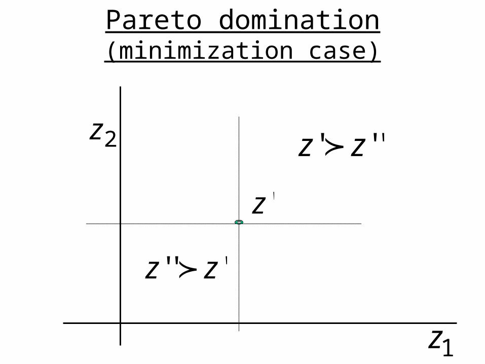
Pareto domination ''' ;,...,2,1 ,'''''' zzmizzzz ii

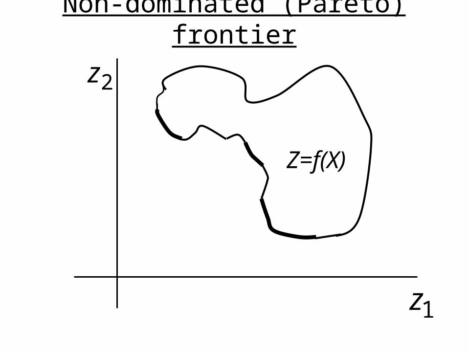
Non-dominated (efficient, Pareto) set

emptysetzzZzZzZP ':':)(

X = feasible set in decision space, mR

Z=f(X)

Feasible set in criterion space

1z

2z

''' zz

'z

Pareto domination (minimization case)

''' zz 2z

1z

1z

2z

Z=f(X)

Non-dominated (Pareto) frontier

Decision maker (DM) is needed to select a unique solution from the set

of Pareto-optimal solutions

Decision maker

Usually the DM is a convenient abstraction only since many different people (advisers, experts, analysts, various stakeholders) influence (or try to influence) the decision.

However, it has sense, and so the concept of the DM is permanently used in the MOO field.

Classification of MCDA methods according to the role of the Decision Maker

MCDA

no-preference methods

a priori preference methods

interactive methods

a posteriori preference

(Pareto frontier)methods

         

 

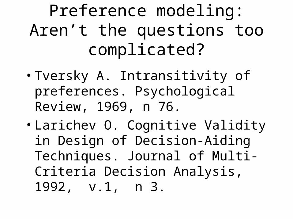
Preference modeling: Aren’t the questions too complicated?

• Tversky A. Intransitivity of preferences. Psychological Review, 1969, n 76.

• Larichev O. Cognitive Validity in Design of Decision-Aiding Techniques. Journal of Multi-Criteria Decision Analysis, 1992, v.1, n 3.

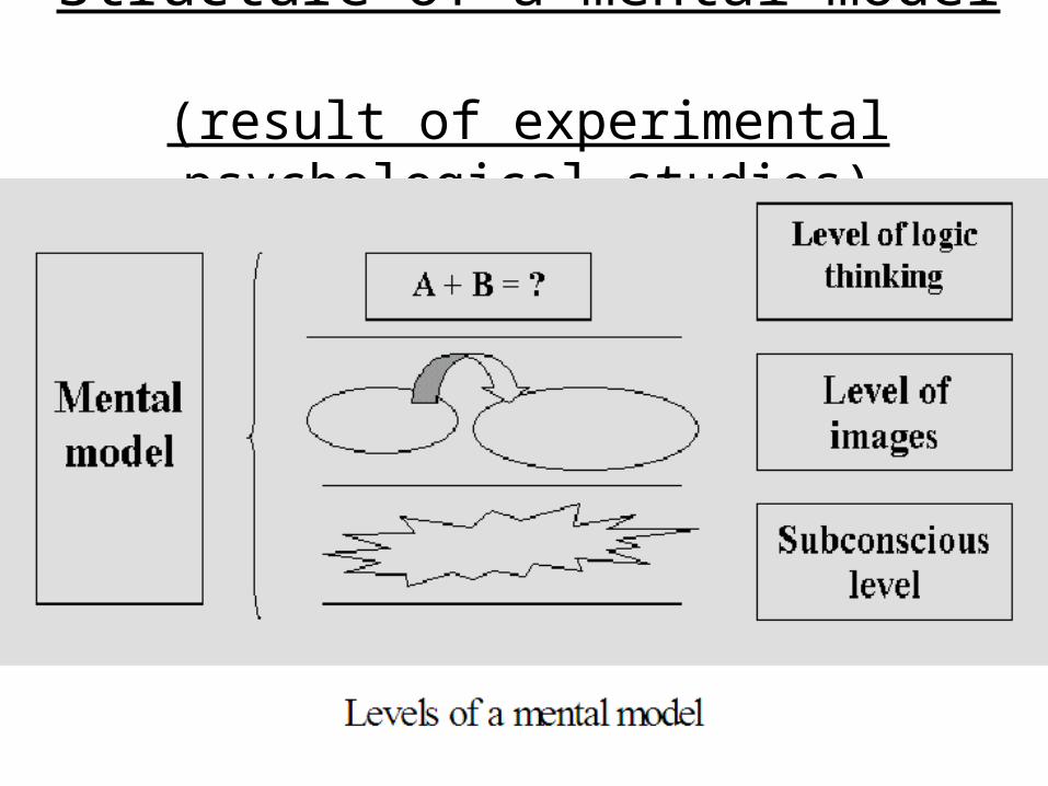
Structure of a mental model (result of experimental psychological studies)

Important feature of the three-levels of human mentality:

The three levels have different pictures of the reality, and much efforts of the human mental activity is related to

coordination of the levels. The conflict between mental levels may result in

non-transitive answers concerning their preference.

Coordinating the levels

A large part of human mental activities is related to the coordination of the levels. To settle the conflict between the levels, time is required.

Psychologists assure that sleeping is used by the brain to coordinate the mental levels. (Compare with the proverb: ``The morning is wiser than the evening'').

In his famous letter on making a tough decision, Benjamin Franklin advised to spend several days to make a choice. It is known that group decision and brainstorming sessions are more effective if they last at least two days.

Coordinating the levels in MOO problems

Thus, to settle the conflict between the levels of one’s mental model in finding a balance between different objectives in a multi-objective optimization problem, he/she needs to keep information on the problem in his/her brains for a sufficiently long time.

Such opportunity is provided by a posteriori (Pareto frontier) methods. The absence of method-related time pressure is an important advantage of them. In contrast, other approaches require fast answers to the questions on preferences.

Pareto frontier methods

Pareto frontier methods are devoted to approximation of the Pareto set and informing the DM concerning it.

In contrast to preference-oriented methods, Pareto frontier methods do not ask multiple questions concerning the preferences, but only inform the DM on the problem.

The first Pareto frontier method in MCO:

generating the Pareto frontier in linear bi-criterion problem (S.Gass and T.Saaty, 1955). Parametric LP methods may be used for solving

bAx Cx,z min)1( 21 zz

where changes from 0 to 1.

     

2z 

1z

Graph was provided to DM!

The feasible criterion values are provided along with the tradeoff rates, which are the most important decision information.

• How to approximate the Pareto frontier

• How to inform the stakeholders about the Pareto frontier

Two main problems must be solved in the framework of the Pareto frontier methods

in the case of m > 2

Two basic ways for informing a stakeholder about the Pareto frontier

• By providing a list of the criterion points that belong to the Pareto frontier

• By visualization of the Pareto frontier

Selecting from a large list of criterion points (more than a dozen) with more

than two criteria is too complicated for a human being, see

• Larichev O. Cognitive Validity in Design of Decision-Aiding Techniques. Journal of Multi-Criteria Decision Analysis, 1992, v.1, n 3.

VISUALIZATION — why it is needed?

Visualization is a transformation of symbolic data into geometric information.

About one half of human brain’s neurons is associated with vision, and this fact provides

a solid basis for successful application of visualization for transformation data into

knowledge.

”A picture is worth a thousand words”..

Visualization can influence all levels of human thinking and simplify by this the

process of coordination.

Requirements that must be satisfied by a visualization technique

To be effective, a visualization technique must satisfy some requirements, which include

(i) simplicity, that is, visualization must be immediately understandable,

(ii) persistence, that is, the graphs must linger in the mind of the beholder, and

(iii) completeness, that is, all relevant information must be depicted by the graphs.

Example: Goal identification with

visualization

Usual goal programming

Goal identification

• DM has to identify the goal (without information on the set Z=f(X)).

0

z*

What really happensThen, by using some distance function, the closest

point of the set Z=f(X) is found.

0

Z=f(X) z0

z*

Goal method based on visualization

1z

2z

Tradeoff information helps to specify the goal

1

2

z

z

f(x*)f(x1)

f(x2)

Goal identification at the Pareto frontier

Once again, criterion tradeoff information is important for decision

maker for identification of the preferable non-dominated feasible

criterion point (goal).

It can be done directly at the non-dominated frontier by using the

computer mouse.

1z

2z

Z=f(X)

Pareto frontier and the feasible goal

One quotation

In a general bi-criterion case, it has a sense to display all efficient decisions by

computing and depicting the associated criterion points; then, decision maker can be

invited to identify the best point at the compromise curve.

B.RoyDecisions avec criteres multiples.

Metra International, v.11(1), 121-151 (1972)

Thus, the question is: Is it possible and is it profitable to visualize the Pareto frontier in the

case of more than two-three criteria?

Interactive Decision Maps technique answers:

Yes, it is possible and profitable.

Interactive Decision Maps (IDM) technique

Edgeworth-Pareto Hull (EPH) of the feasible criterion set

mp RZZ

)()( ZPZP p

It holds

is

      

        

P(Z)

f(X) pZ

 

1z

2z

z*

Ideal point and Edgeworth-Pareto Hull

mp RZZ )()( ZPZP p

Two spaces in MOO problems

• Decision space:

• Feasible set

• Criterion space:

• Feasible set in criterion space

nR

nRX

mR

)(XfZ

The IDM technique is a tool for visualization of multi-objective (m>3) Pareto frontier. It is based on approximation of the EPH and subsequent interactive visualization of the Pareto frontier by using various collections of bi-objective slices of the EPH.

Decision map is a collection of bi-objective slices of the Pareto frontier (or EPH) in the case of three criteria.

Interactive Decision Maps technique provides interactive visualization and animation of the decision maps.

Thus, it is a tool for Pareto frontier visualization in the case of more than of three criteria.

An example problem for IDM software demonstration

The problem

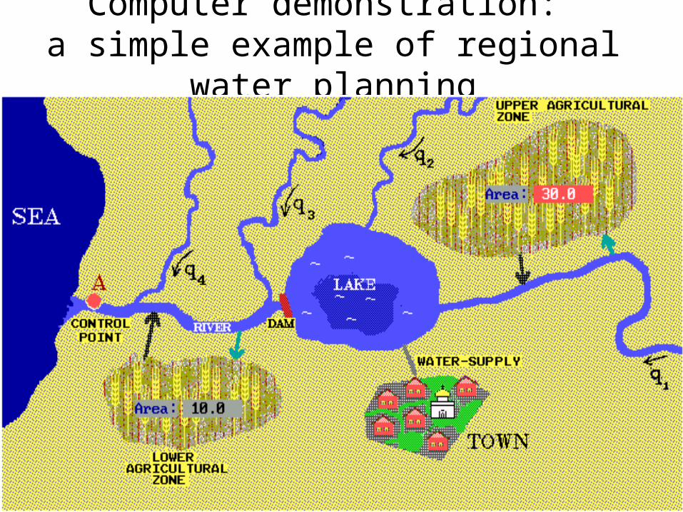
The problem of economic development of the region is studied. If the agricultural (to be precise, grain-crops) production would increase, it may spoil the environmental situation in the region. This is related to the fact that the increment in the grain-crops output requires irrigation and application of chemical fertilizers. It may result in negative environmental consequences, namely, a part of the fertilizers may find its way into the river and the lake with the withdrawal of water. Moreover, shortage of water in the lake may occur during the dry season.

Two agricultural zones are located in the region. Irrigation and fertilizer application in the upper zone (located higher than the lake) may result in a drop of the level of the lake and in the increment in water pollution. Irrigation and fertilizer application in the second zone that is located lower than the lake may also influence the lake. This influence is, however, not direct: irrigation and fertilizer application in the lower zone may require additional water release from the lake into the river (the release is regulated by a dam) to fulfill the requirements of pollution control at the monitoring station located in point A .

The model

The model consists of three sub-models: • model of agricultural production;• water balances and constraints;• pollution balances and constraints.

The production in an agricultural zone is described by a technological model, which includes N agricultural production technologies. Let xij, i=1,2...,N, j=1,2, be the area of the j-th zone where the i-th technology is applied.

The areas xij are non-negative and are restricted by the total areas of zones

N

ijij jbx

12,1 ,

The i-th agricultural production technology in the j-th zone is described by the parameters aij

k, k=1,2,3,4,5, given per unit area, where aij1 is

production, aij2 is water application during the dry period, aij

3 is fertilizers application during the dry period, aij

4 is volume of the withdrawal (return) flow during the dry period, aij

5 is amount of fertilizers brought to the river with the return flow during the dry period. Thus, one can relate the values of production, pollution, etc. to the distribution of the area among technologies in the zone

where zj1 is production, zj

2 is water application during the dry period, zj3

is fertilizers application during the dry period, zj4 is volume of the

withdrawal (return) flow during the dry period, zj5 is amount of

fertilizers brought to the river with the return flow during the dry period in the j-th zone.

N

iij

kij

kj kjxaz

15,...,1 ,2,1 ,

The water balances are fairly simple. They include changes in water flows and water volumes during the dry period. The deficit of the inflow into the lake due to the irrigation equals to z1

2 z14. The

additional water release through the dam during the dry period is denoted by d. It is supposed that the release d and water applications are constant during the dry season.

Let T be the length of the dry period. The level of the lake at the end of the dry period is approximately given by

L(T) = L (z12 z1

4 + d)/, where L is the level without irrigation and additional release, and is a

given parameter.

Flow in the mouth of the river near monitoring point A denoted by vA equals to vA

0+(d z22 + z2

4)/T, where vA0 is the normal flow at point A.

The constraint is imposed on the value of the flow vA vA*, where the value vA* is given. Thus, the following constraint is included into the model

vA0+(d z2

2 + z24)/T vA*.

The increment in pollution concentration in the lake denoted by wL is approximately equal to z1

5/ , where is a given parameter.

The pollution flow (per day) at the point A denoted by wA is given by z2

5 /T + qA0 , where qA

0 is the normal pollution flow. It means that we neglect the influence of fertilizers application in the upper zone on pollution concentration in the mouth.

Then, the value of wA equals to (z25 /T + qA

0 ) / vA .

The constraint wA≤wA* where wA* is given is transformed into the linear constraint (z2

5 /T + qA0 )

≤wA* vA or

z25 /T + qA

0 ≤wA*( vA0+(d z2

2 + z24)/T).

Decision variables and criteria

The decision variables are allocations of land between different technologies in the agricultural zones as well as the additional water release through the dam.

For the criteria, any collection of the variables of the model can be used. In the following demonstration, five economic and environmental criteria are used.

Computer demonstration: a simple example of regional water planning

Demonstration of software(IDM + Feasible Goals Method)

Summary of demonstration

The IDM technique applies the same kind of visualization as the topographical maps, which are used more than 300 years. This evidence (as well as psychological experiments) prove that the IDM technique is simple enough to be understood, uses to linger in the mind of the beholder and provides all relevant information.

Mathematics of the IDM technique

      

        

P(Y)

f(X) pY

 1y

2y

Illustration of the EPH

The EPH is approximated by a polytope plus the non-negative cone. We apply the Estimation Refinement (ER) method proposed by V.Bushenkov and A.Lotov in the beginning of the 1980s. It is now the main computational tool for polyhedral approximating the multidimensional convex sets (including the EPH).

We start with approximating of convex compact bodies.

Approximating the EPH the convex case

Non-adaptive approximation methodsPolyhedral approximating of convex compact bodies

is often based on computing the values of the support function of the approximated body C, i.e.

gC (u) = max {<u, x>: x C},

for a given finite system of directions {u1, u2, …, uL}. It is clear that such a grid neglects the actual shape of the body being approximated. For this reason, the approach based on the a priori directions is not the best one. G.Sonnewend (1983) proved that the methods using such directions are not optimal. They require too many evaluations of the support function; polytopes constructed by them have too many vertices and faces.

Adaptive approximation of convex bodies

The adaptive methods, which adapt the directions {u1, u2, …, uL} to the form of the approximated body, i.e. the directions identified in the approximation process. It was proven that the adaptive methods (that satisfy some conditions) are asymptotically optimal in the sense, which will be described a bit later.

The ER method is the first of the adaptive methods for polyhedral approximating the compact convex bodies for more than two dimensions.

The ER method

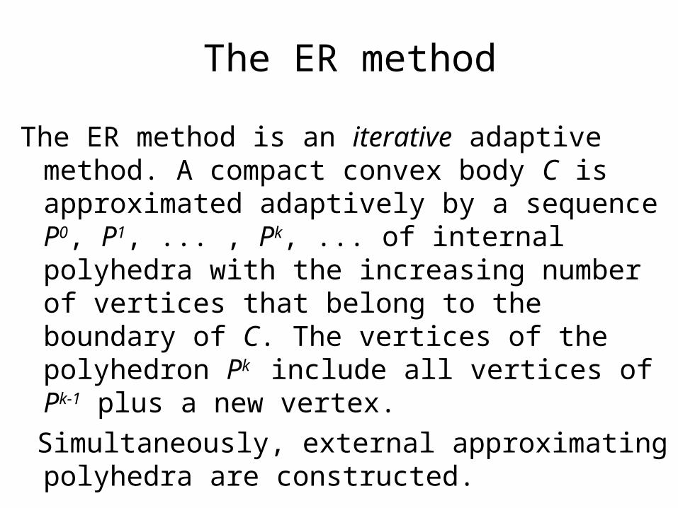
The ER method is an iterative adaptive method. A compact convex body C is approximated adaptively by a sequence P0, P1, ... , Pk, ... of internal polyhedra with the increasing number of vertices that belong to the boundary of C. The vertices of the polyhedron Pk include all vertices of Pk-1 plus a new vertex.

Simultaneously, external approximating polyhedra are constructed.

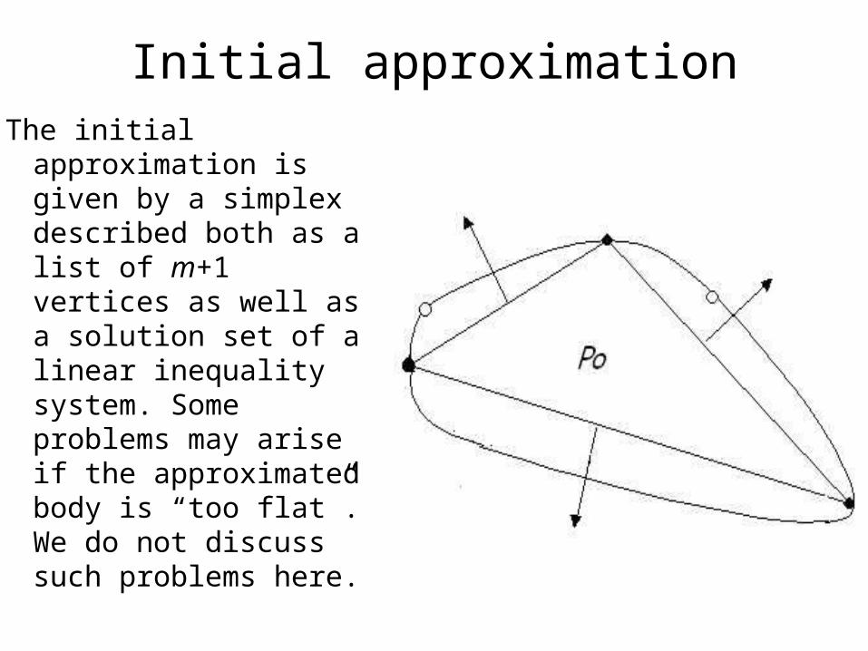
Initial approximationThe initial approximation

is given by a simplex described both as a list of m+1 vertices as well as a solution set of a linear inequality system. Some problems may arise if the approximated body is “too flat”. We do not discuss such problems here.

Math description of the ER method

Let U(P) denote the finite set of unit outer normals to the facets of the approximating internal polyhedron. The finite set U(P) is defined if the polyhedron P is given in the form of a solution set of a linear inequality system.

Let us describe the (k + 1)-th iteration of the method. Prior to the iteration, we should have constructed the internal polyhedron Pi

k in the form of a solution set of the linear inequality system Dk y≤dk and in the form of a list of its vertices; the external polyhedron Pe

k must be given in the form of a solution set of a linear inequality system.

Step 1

The direction u* from U(Pk) is found that solves

If then stop.

Else the point y* is selected such as

}; )( :))()(( max{ k

PC PUuugug k

*)(*)( ugug kPС

*).(**, ugyu С

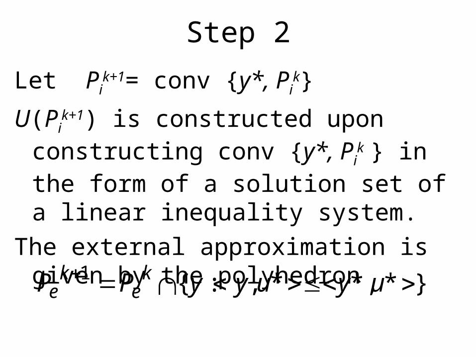
Step 2

Let Pik+1= conv {y*, Pi

k}

U(Pik+1) is constructed upon constructing conv

{y*, Pik } in the form of a solution set of a

linear inequality system.

The external approximation is given by the polyhedron

}**,*,:{1 uyuyyPP ke

ke

Constructing the convex hull of a polyhedron and a point

Stable variant of beneath-beyond methodParticular methods that implement the beneath-beyond

scheme differ in the way they solve the three following problems:

• How to determine whether a facet is visible from a point;• How to determine whether two facets are adjacent or not;

and• How to transform the representation of the polyhedron

into the convex hull.A stable form of the beneath-beyond method was developed

by O.Chernykh in 1986 and is based on the convolution of a linear inequality system. The convolution of such systems was proposed by Fourier in 1826 and modified in Russia in 60s by S.N.Chernikov.

Approximation precisionNote that both the internal and the external polyhedra are

constructed. By this, the approximation precision is controlled automatically by evaluating the value

as well as graphically, since

Moreover, the Hausdorff distance between sets C1 and C2 can be studies, i.e. the value δ(C1, C2) =

max { sup {d (x, C2): x C1 }, sup {d (x, C1): x C2 } }.It was proven that

for any convex compact body C.

0),(lim

CPk

k

*)(*)( ugug kPС

kk PCP ˆ

Theory of polyhedral approximation

Polyhedra of best approximation

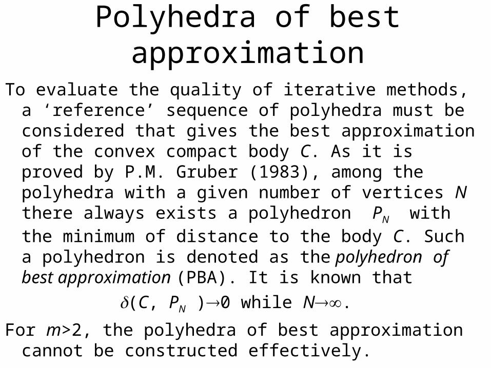
To evaluate the quality of iterative methods, a ‘reference’ sequence of polyhedra must be considered that gives the best approximation of the convex compact body C. As it is proved by P.M. Gruber (1983), among the polyhedra with a given number of vertices N there always exists a polyhedron PN with the minimum of distance to the body C. Such a polyhedron is denoted as the polyhedron of best approximation (PBA). It is known that

(C, PN )0 while N.

For m>2, the polyhedra of best approximation cannot be constructed effectively.

Known estimatesIf the body C has a sufficiently smooth boundary, there exist positive

constants kC and KC such that

kC / N 2/(m-1) (C, PN) KC / N 2/(m-1)

(Bronshtein and Ivanov, 1975, Schneider and Weacker, 1981, and Gruber and Kendrov, 1982).

Thus, the distance of the PBA from the approximated body C decreases with the order of convergence 2/(m-1).

Examples

• for m=2 one obtains 1/N2

• for m=3 one obtains 1/N

• for m=5 one obtains 1/N0.5

• for m=7 one obtains 1/N1/3

The PBA as an ideal sequence

The PBA cannot be found, but their sequence can be used as the ‘reference’ sequence of approximating polyhedron in a general case. Note that the PBA do not provide an iterative sequence at all, since the vertices of PN are not related to vertices of PN-1. Thus, one can not even dream concerning an iterative procedure that constructs the sequence of PBA.

However, it is important to remember that the PBA-based ‘reference’ sequence of polyhedra provides an ideal that is not feasible in reality.

Hausdorff class of methodsThus, any sequence of polyhedra generated by

approximation methods can be compared with the sequence of PBA. Note that the polytopes generated by an iterative method cannot approximate the body C better than PBA.

G.Kamenev (1992 and 1993) introduced the notion of the Hausdorff class of methods for iterative polyhedral approximating of compact convex bodies. A method is denoted as a Hausdorff method with a constant γ > 0 for a body C, if it results in a sequence of polyhedra {Pk}, k = 0, 1, ... for which it holds

(Pk, Pk+1) γ (Pk, C), k = 0, 1, ...

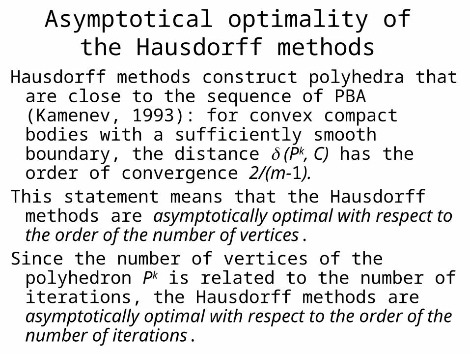
Asymptotical optimality of the Hausdorff methods

Hausdorff methods construct polyhedra that are close to the sequence of PBA (Kamenev, 1993): for convex compact bodies with a sufficiently smooth boundary, the distance (Pk, C) has the order of convergence 2/(m-1).

This statement means that the Hausdorff methods are asymptotically optimal with respect to the order of the number of vertices.

Since the number of vertices of the polyhedron Pk is related to the number of iterations, the Hausdorff methods are asymptotically optimal with respect to the order of the number of iterations.

Asymptotic efficiency of an optimal iterative method

Since the Hausdorff methods are optimal with respect to the order of the number of vertices, it is interesting to know about the ratio of distances (Pk, C) and (PN, C). Let us consider a sequence of polyhedra F = {Pk}, k = 0, 1, .... The value

is denoted as the asymptotic efficiency of the method that was used for generating the sequence F. Evidently, that h(F) = 1 can be achieved by the sequence of PBA. For a not optimal sequence it holds h(F) = 0. For an optimal sequence, it holds 0 ≤ h(F) < 1.

It was shown that for the sequence produced by a Hausdorff method for convex compact bodies with a sufficiently smooth boundary, it holds

),(

),( inflim)(

k

N

k PC

PCF k

4

11)(

2

F

Properties of the ER method

Main theoretical results concerning the ER method

Kamenev (1994) proved that, for any compact convex body with a sufficiently smooth boundary, the ER method is a

Hausdorff method with some constant γ and that

asymptotically (while N) the value of γ is close to 1.

Thus, for convex compact bodies with a sufficiently smooth boundary, the ER method provides the same (as PBA) order of asymptotical convergence, i.e.

(C, Pk) ~ Const / Nk 2/(m-1)

Moreover, it holds

.4

1)( F

Asymptotic optimality in respect to the order of calculation of the

support function

Recently Kamenev and Efremov proved that the ER method is asymptotically optimal in respect to the order of the number of computing the support function. Till now, it is the unique property of the ER method .

Application of the ER method for approximating the EPH

In the process of approximating the EPH in the convex case, the only special feature of the ER method consists in constructing the initial approximation. In contrast to approximating a compact body, the initial approximation is the nonnegative cone with the vertex in a Pareto optimal criterion point.

Real-life environmental applications

What is it real-life application?

Real-life application of a method is an application characterized by a relatively long-time use of the methods by decision makers for exploration of real-life decision problems without a direct support of the author of the method.

Methodology for decision screening

Remind that any decision process consists of the two main phases. The first one is the early decision screening, i.e. selecting a small number of decision alternatives from the whole variety of possible alternatives for further exploration. The second stage is related to the final choice among a small number of alternatives on the basis of their detailed exploration.

DSS for Water quality planning in the

Oka River (Russian Federal Programme

Revival the Volga River)

The Problem

The water quality problem studied here is related to the selection of an efficient strategy of investment into the wastewater treatment facilities that must be constructed in a large river basin to improve the water quality. Several regions are located in the river basin.

The problem is how much investment is needed and how to allocate the investment between regions, what kind of wastewater treatment technologies to apply, etc.

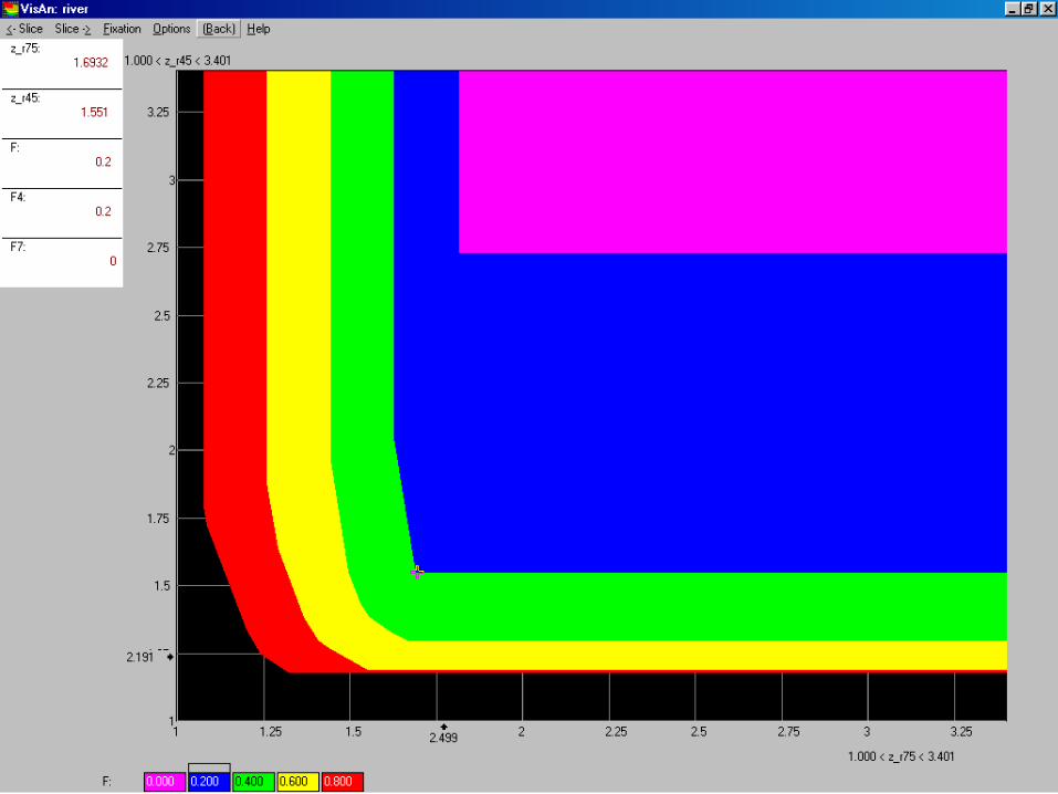
DSS allows user to specify two to seven performance indicators from the list to be the screening criteria. Constraints on the indicator values can be imposed.

Here the total cost of the project, the investment in the fourth region and the investment in the seventh region have been already specified to be screening criteria.

Once a feasible goal is specified, a strategy related to it is computed and displayed in the central column of the table.

Evolutionary study

Opportunity of evolutionary study of the problem is provided:

if decision maker is not satisfied with the strategy or loosely wants to search for additional strategies by playing with the system, he/she can return to the initial criteria specification table and specify a new set of criteria and/or impose new constraints on performance indicators.

Exploration of pollution abatement cost in the Electricity Sector – Israeli case study

(jointly with D. Soloveitchik and others fromMinistry of National Infrastructures, Israel)

Was used by Ministry of National Infrastructures of Israel during 2001-2005.

Several hundreds of pollution reduction alternatives for the electricity sector were developed for the period 2003 - 2013. The

criterion values were computed by application of a complicated non-linear mathematical

model. Then, the IDM-based screening was applied in the form of the Reasonable goals

method (RGM)

Few words concerning RGM

Example: real estate on sale

For illustrative purposes, let m=2 (criterion points are displayed in the plane). Non-dominated points are given by crosses.

Enveloping the criterion points

Approximating the Edgeworth-Pareto hull of the convex hull (the so-called CEPH)

Pareto frontier is analyzed by user and a preferred combination of criterion values

(reasonable goal) is identified

The alternatives that are close to the goal are selected

General case (from 3 to 8 criteria)

Visualization of the Pareto frontier

is based on approximation of the EPH of the convex hull of criterion points and application of the Interactive Decision

Maps technique for the interactive analysis of the frontiers of the slices.

Let us return to Israeli electricity production problem. Five selection criteria were used:

• percent of CO2 reduction (CO2_%);

• percent of NOx reduction (NOx_%);

• additional total cost (NPV_D);

• marginal abatement cost (NPV_DC($));

• percent of growing average cost of electricity (AV.C_%).

Decision map displays tradeoff between CO2% and NPV_D for several levels of NOx reduction as well as given levels of marginal abatement cost and percent of growing average cost

of electricity

Searching for trans-boundary air pollution control strategies

Acid rain in Finland, Estonia and a part of Russia is studied. In 1991 the government of Finland has decided to develop a program of environmental investment in areas that are the sources of trans-boundary air pollutants deposited in Finland. Finnish specialists expressed interest in using the FGM-based software to solve this kind of problems. Experts of the governments of the countries involved can study the feasibility frontiers of sulfur deposition rates and abatement costs in the individual countries as well as the tradeoffs among these criteria, develop appropriate feasible combinations of criterion values and associated abatement strategies.

DataIn 1988 the Finnish-Soviet Commission for Environmental Protection

established a joint program for estimating the flux of air pollutants emitted close to the border between the countries. It consists of the estimation of emissions, model computing of trans-boundary transport of pollutants, analysis of observational results from measurement stations and conclusions for emissions reductions.

The emissions inventory includes sulfur, nitrogen and heavy metals, but in this study only sulfur deposition is taken into account. Emission data approved by the Finnish-Soviet Commission were used as inputs of our model.

Depositions and transport of sulfur were calculated by applying the long-range transport model for sulfur developed at the Western Meteorological Center of the European Monitoring and Evaluation Program (Oslo, Norway).

The modelThe model consists of the sulfur transportation model and the sulfur

abatement costs functions.A sulfur transportation matrix indicates how the emission in one area is

transported in the atmosphere for deposition in another. The large numbers on the diagonal show that their own sources of

pollution play an important role in each region.

Let E and Q denote the vectors of annual emission and deposition of sulfur, respectively, and let A stand for the matrix given in the table and B for the vector of exogenous deposition. The sulfur transportation model can then be expressed in vector notation as

Q=AE+B.

Information about future regional emissions E, which depend on abatement cost, was developed by Finnish specialists, too.

Piecewise linear functions used for the annual sulfur abatement costs functions include both capital and

operating costs, measured in million of Finnish marks.

Decision variables and screening criteriaDecision variables are the emissions in seven regions under

consideration.A list of performance indicators was formulated. These

indicators can be used as possible screening criteria. User can apply several of indicators from the following six

groups: • sulfur abatement cost in each sub-region;• abatement cost in Finland, in the nearby region of

Russia, and in Estonia;• total abatement cost for the whole territory;• average sulfur deposition in each sub-region;• maximal average depositions in the sub-regions of

Finland, Russia, and Estonia;• maximal average depositions in the whole territory.

Exploration of the modelLet us consider an example. Suppose the user has specified

three criteria:• abatement cost in Finland (CF, in million Finnish mark);• total abatement cost (TC, in billion Finnish mark);• maximal deposition rate in Finland (PF, in gram per square

meter).

It is assumed that the decrement in the second and the third criteria values are preferable. The direction of improvement of the first criterion is not specified. Let us assume that the following constraints were imposed:

• the deposition rate in Northern Finland must be not greater than 0.4 gram per square meter;

• the deposition rate in Central Finland must not be greater than 0.5 gram per square meter.

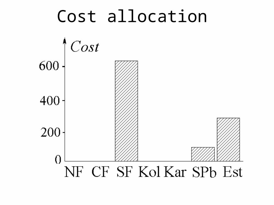
In Figure several frontiers of the variety of feasible criterion vectors are depicted in the plane of the criterion CF (investment in Finland) and the criterion PF (maximum deposition rate in Finland) for several values of total abatement cost.

The range of total costs in the whole region is between zero and 4.1 billion FIM. The following total cost values were selected: 0.25, 0.5, 0.75, 1.00, 1.25, 1.50, 1.75, and 2.00 billion FIM.

Cost allocation

Real-life application of the results

Inferences of our research, i.e. the potential profitability for Finland of an environmental investment in Russia, were discussed by us in the 1990s with officials in both countries. They expressed interest, but refused to use the software.

However, in September 2001, Presidents of Finland and Russia decided that Russian debt to Finland (about US$500 million) may be partially used for decreasing the emission of air pollutants in St. Petersburg area.

Could it happen that our research has influenced in some way the concepts of Finnish and Russian officials?

Web-based real-life application

Application server based on the IDM technique was developed(Web RGDM software)

http://www.ccas.ru/mmes/mmeda/rgdb/

index.htm

Scheme of the Web RGDB application server

The Web application server was used as a part of DSS developed by

Jörg Dietrich and Andreas H. Schumann, Ruhr University Bochum,

in the framework of the project

Participatory Decision Support for Integrated River Basin Planning

(2003-2004)

Funding: German Federal Ministry of Education and Research

DSS was applied in group decision support for planning the Werra River Basin

Weser

Rhein

Ems Elbe

Werra

Input of Decision Matrix

For the Participatory Decision Support System, a specialized form of the Web server was developed. It can support negotiations of people.

They can identify preferable reasonable goals and, may be, obtain associated alternatives. Then, they

can try to close the gap between their goals.

Architecture of the Web-based DSS

The plan of Werra basin management was developed. Unfortunately, ordinary people (lay stakeholders) were excluded from the

decision process.

Next German project (under preparation) is related to strategies of defending the sea shore in China (mouth of Yellow River).

Two main tasks to be solved in the framework of e-participation in

environmental decision problems

• a) informing lay stakeholders on environmental and other public decision problems (especially on possible strategies for solving the problems); and

• b) supporting negotiations.

Web tools based on the RGM/IDM technique (RGDB) can help lay

stakeholders better understand the feasibility frontiers and express

preferences by selecting one or several strategies that best fit their concerns.

Current Project: E-DEMOCRACIA-CM

(Madrid community).

A framework for participatory group decision support using Pareto

frontier visualization, goal identification and arbitration

R. Efremov, D. Rios Insua,(University of Rey Juan-Carlos, Madrid)

A. Lotov

(Dorodnicyn Computing Centre of Russian Academy of Sciences, Moscow)

A participatory decision making process is divided into two stages:

• At the first stage, stakeholders express their preferences in the form of feasible (or reasonable) goals

• At the second stage, the preference information is used in an arbitration procedure to construct the group decision.

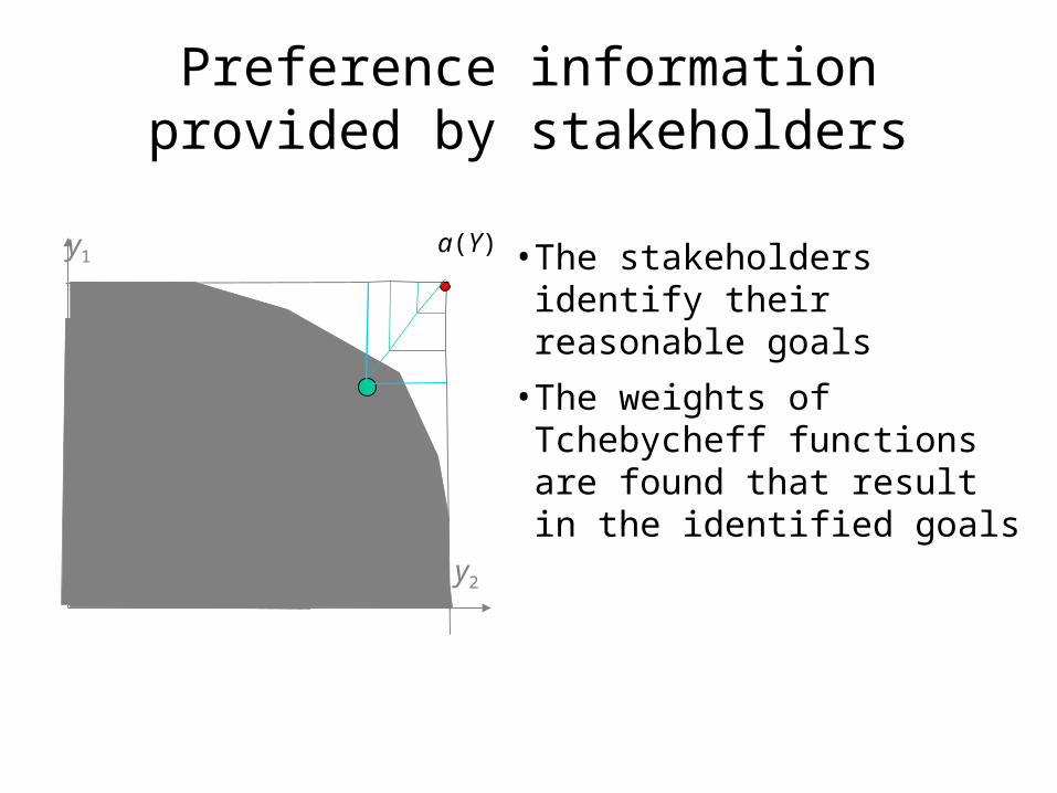
Preference information provided by stakeholders

a(Y)

y(1)

y1

y2

• The stakeholders identify their reasonable goals

• The weights of Tchebycheff functions are found that result in the identified goals

Goal-based arbitration scheme

a(Y)

y(1)

y1

y2

y(2)

The arbitration scheme is based on averaging the weights of Tchebycheff functions

Alternative forms of arbitration rules were developed and experiments

were carried out

Experimental application: group decision support tool for selecting a

hostel in London town

Criteria :

LocationLocation

SecuritySecurity

PricePrice

CleanlinessCleanliness

Staff (service)Staff (service)

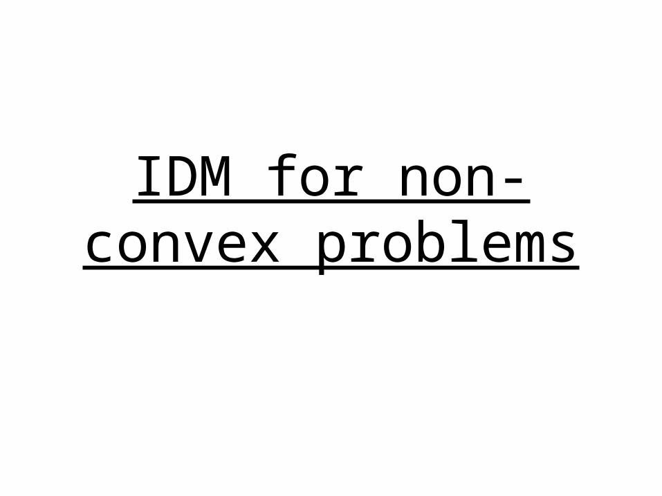
IDM for non-convex problems

The main problems that may arise in the non-linear

case:

1. non-convexity of the set Y=f(X); and

2. time-consuming algorithms for global scalar optimization.

Approximation for visualizationThe EPH is approximated by the set T* that is the union of the non-negative cones

with apexes in a finite number of points y of the set Y=f(X). The set of such points y is called the approximation base and is denoted by T.

Important! Multiple slices of such an approximation can be computed and displayed fairly fast.

mRy

Visualization example for 8 criteria

Goal identification

Any system of criterion points can be visualized in this way

(software is downloadable from our Web site).

Let us consider now the methods we

use for approximating the EPH in the non-linear non-convex case.

Group of Prof Yu. Evtushenko develops methods for approximating the EPH in the case of Lipschitz functions. In contrast, we approximate the EPH in the MOO problems with criterion functions given by black-box models (FEM/FDM modules and other simulation modules). Thus, the Lipschitz constants are unknown (or may not exist at all). The only feasible operation is variation of inputs and collecting the related outputs.

We apply hybrid methods that include:

1) global random search;2) adaptive local optimization;3) importance sampling;4) genetic algorithms.

Statistical tests of the approximation quality play the leading role in approximation process.

Statistical testsQuality of an approximation T* is studied

by using the concept of completeness hT = Pr {x X results in f(x)  T*}.

We estimate Pr { hT > h* } for a given reliability by using a random sample

HN = {x1, … ,  xN}. Let hT

(N)= n/N, where n=|f(xi)  T*|. Then, hT

(N) is a non-biased estimate of hT .Moreover, h *=hT

(N) – (– ln (1 – ) / (2N) )1/2

describes the confidence interval.

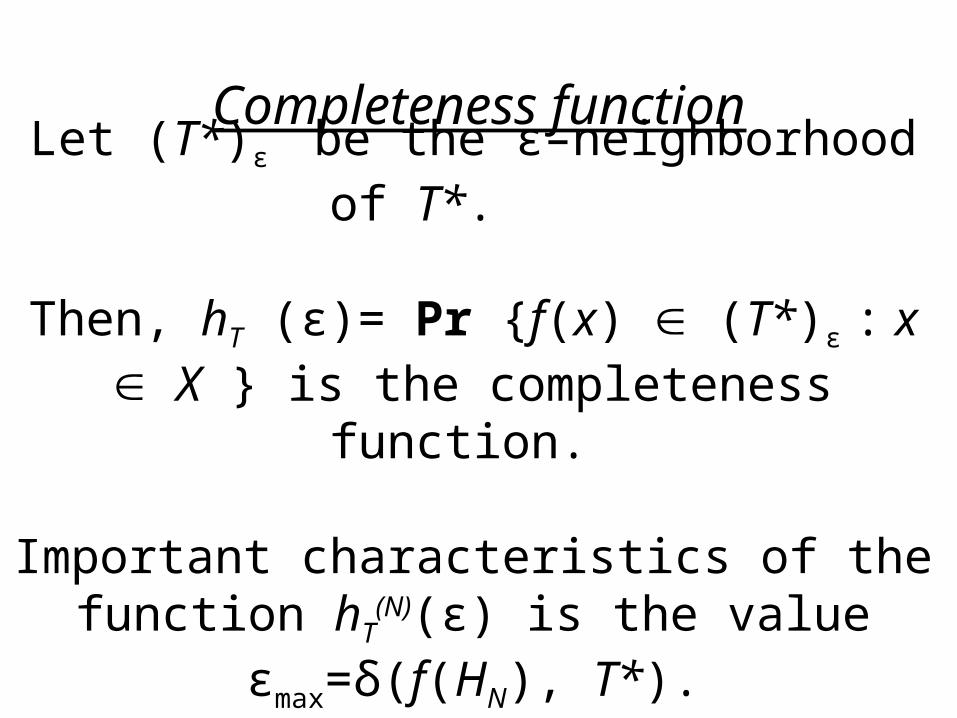
Completeness function

Let (T*)ε be the ε–neighborhood of T*.

Then, hT (ε)= Pr {f(x)  (T*)ε : x X } is the completeness function.

Important characteristics of the function hT(N)(ε)

is the value εmax=δ(f(HN), T*).

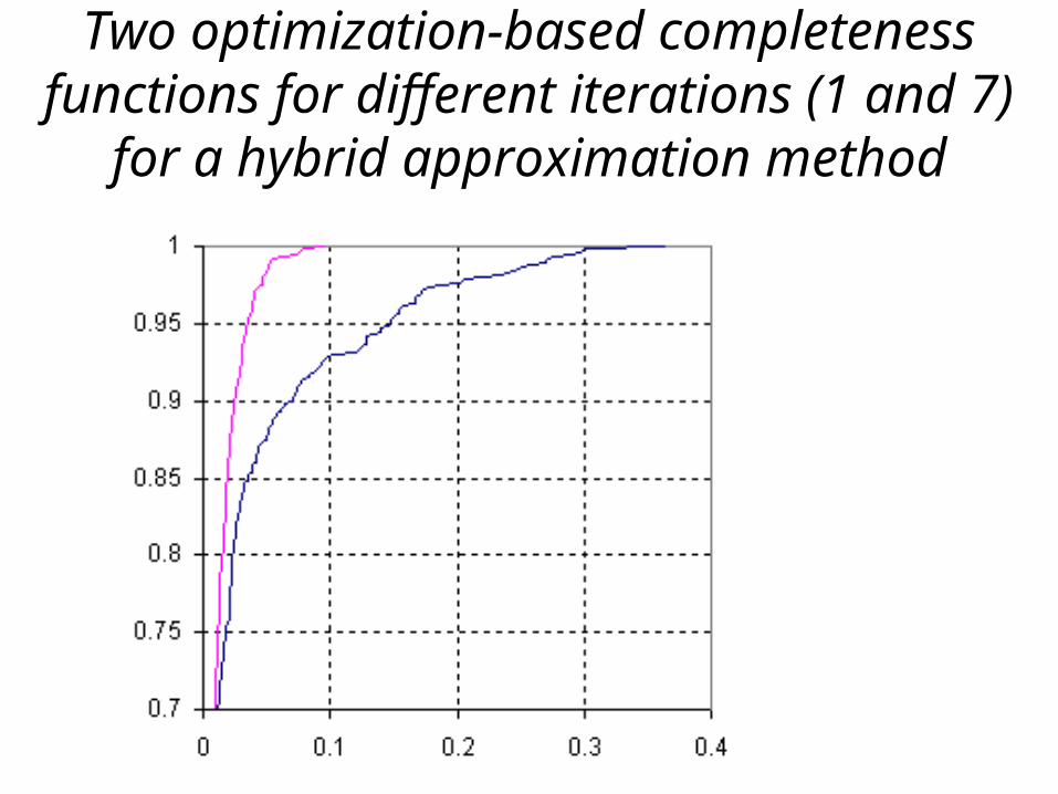
The optimization-based completeness

Optimization-based completeness function is hT (ε) = Pr{f(Φ(x0)) (T*)ε : x X }

where Φ:X → X is the “improvement” mapping,

which is based on local optimization of a scalar function of criteria. The mapping moves f(Φ(x0))

closer to the Pareto frontier. We generate a random sample HN {x1, … ,  xN} and compute

hT(N)(ε)=n(ε)/N, where n(ε)=|f(Φ(xi

0))  (T*)ε|.

Two optimization-based completeness functions for different iterations (1 and 7) for a hybrid

approximation method

One-phase method

An iteration. A current approximation base T is given. 1. Testing the base T. Generate a random sample HN X , compute hT

(N)(ε). If hT(N)(ε) (or some

values as hT(N)(0) and εmax=δ(f(HN),T*) in

automatic testing) satisfy your requirements, stop.

2. Forming new base. Form a list that includes points of T and sample points that not belong to T*, exclude dominated points. By this a new approximation base is found. Start next iteration.

Two-phase method

An iteration. A current approximation base T is given. 1. Testing the base T. Generate a random sample HN X , compute Φ(HN). If hT

(N)(ε) (or some values as hT

(N)(0) and εmax=δ(f(Φ(HN)),T*) in

automatic testing) satisfy your requirements, stop.

2. Forming new base.

Start next iteration.

Three-phase method

An iteration. Current base T and an approximation of P(X) denoted by B must be given 1. Testing the base T. Generate two random samples H1X and H2 B, compute Φ(H1) and Φ(H2). If hT

(N)(ε) satisfies your requirements,

stop.

2. Forming new base. 3. Forming new approximation of P(X) using extreme statistics in decision space. Start next iteration.

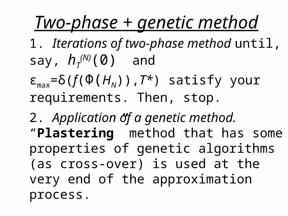
Two-phase + genetic method

1. Iterations of two-phase method until, say, hT(N)

(0) and εmax=δ(f(Φ(HN)),T*) satisfy your requirements. Then, stop.

2. Application of a genetic method. “Plastering” method that has some properties of genetic algorithms (as cross-over) is used at the very end of the approximation process.

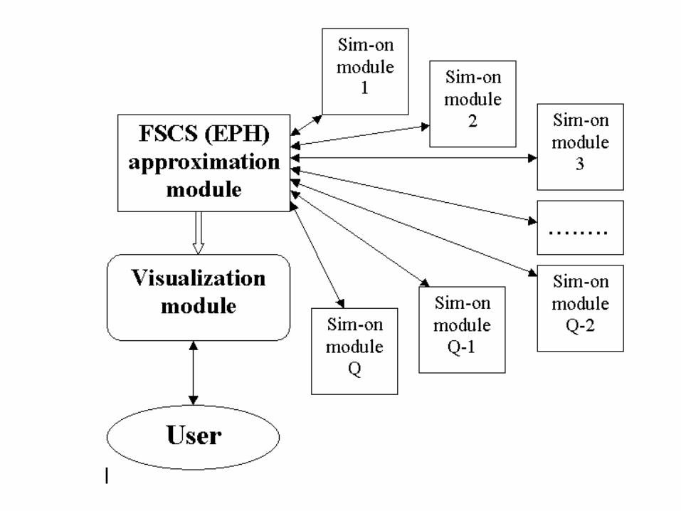
Parallel computing

The method has the form that can be used in parallel computing.

Thus, it can be easily implemented at parallel platforms including

processor clusters, supercomputers or grid networks. It is sufficient to separate data generation and data

analysis(Research in the framework of contract with Russian

Federal Agency for Science).

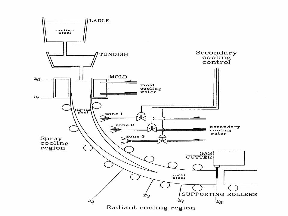
Methodological applications

Study of a cooling equipment in continuous casting of steel.

The research was carried out jointly with researchers from University of

Jyvaskyla, Finland.

CriteriaJ1 is the original single optimization criterion: deviation from the desired surface temperature of the steel strand must be minimized.J2 to J5 are the penalty criteria introduced to describe violation of constraints imposed on : J2 – surface temperature; J3 – gradient of surface temperature along the strand;

J4 – on the temperature after point z3; and J5 – on the temperature at point z5.

J2 to J5 were considered in this study.

Description of the module

FEM/FDM module was developed in Finland,by researchers from University of Jyvaskyla. Properties of the model: 325 control variables that describe intensity of water application.

Properties of local simulation-based optimization:one local optimization required about 11-12 calculations of the gradient and about 1000-2000 additional calculations of the value of f(x).

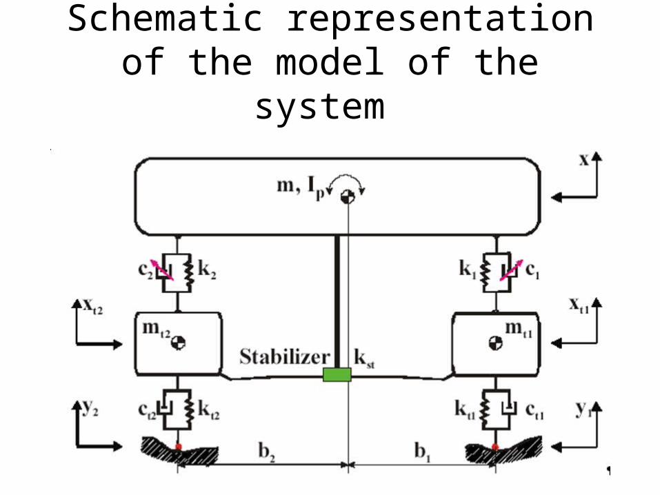
Designing controllers for semi-active suspension system with added stabilizer

for new generation of cars

Requested by STMicroelectronics, Italy-France, jointly with Moscow Research Lab of STMicroelectronics

Schematic representation of the model of the system

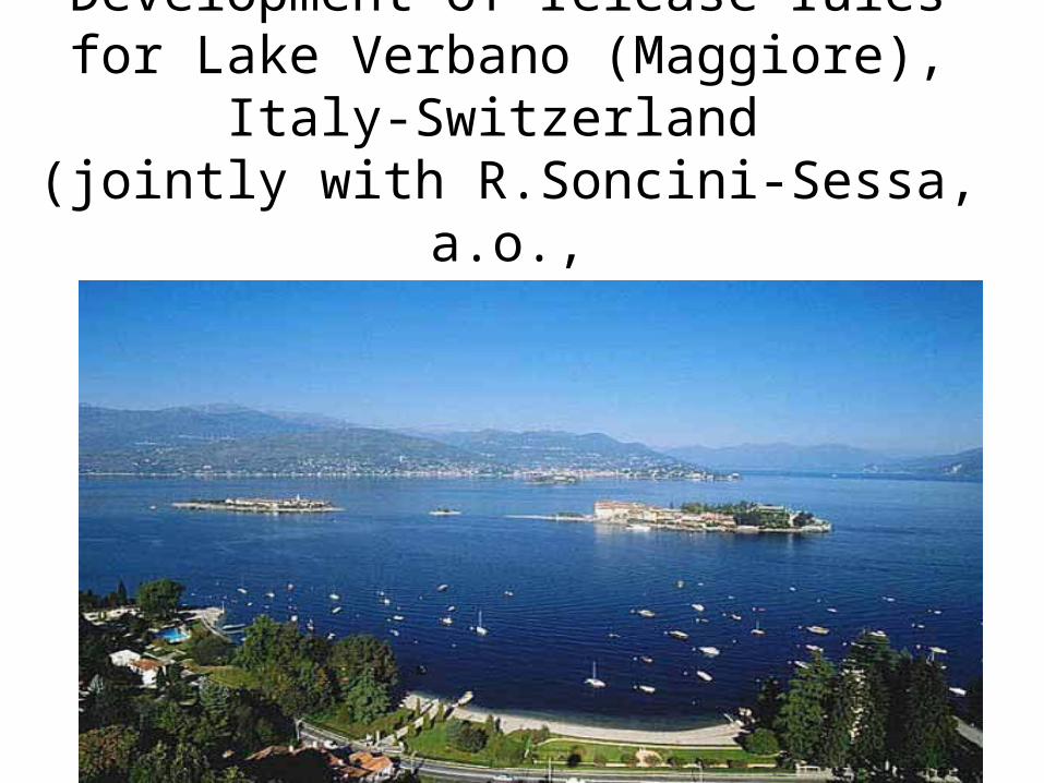
Real-life applications

Development of release rules for Lake Verbano (Maggiore), Italy-Switzerland

(jointly with R.Soncini-Sessa, a.o., Politecnico di Milano )

Scheme of the basin

Choice criteriaY 1 is level of the lake

Y 2 is deficit of water for irrigation

Y 3 is environmental damage

Y 4 is income of hydropower production

Criterion values for a particular variant of release rules were evaluated by simulating the rules for historical records of inflow (daily) into the Lake Verbano during 25 years.

An example of decision map

Current real-life studies

Development of release rules for Angara hydropower stations

Criteria:• Electricity production• Level of the Lake Baikal• Requirements of transportation • Level of the Angara near large cities, etc.Historical data on the inflow into the Baikal

Lake collected for about 25 years are used to evaluate the performance criteria.

MULTI-CRITERIA IMPROVEMENT OF LAKE WATER QUALITY BY USING LINEARIZATION OF RESPONSE

SURFACES WITH LARGE NON-LINEAR, PROCESS-BASED MODELS

Jointly with A.Castelletti and R.Sencini-Sessa from Politecnico di Milano

Water Quality Rehabilitation

Draft tube mixers

Surface pumps

Bottom pumps

INTERVENTIONS

Algal blooms Turbidity

Benthic metal release

……

High temperature

ISSUES

……

Decisions (Design parameters)

Design parameters: Thrust

Number

×

×

×

Position

e.g.

: number of mixers

: position of the mixers

feasibility set

decision vector

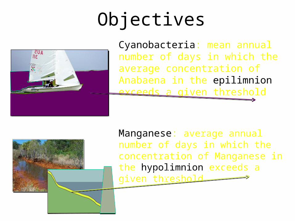
ObjectivesCyanobacteria: mean annual number of days in which the average concentration of Anabaena in the epilimnion exceeds a given threshold

Algal blooms

Benthic metal release Manganese: average annual number of days in which the concentration of Manganese in the hypolimnion exceeds a given threshold

Study Site: Googong reservoir (Australia)

• Volume 121 X 106 m3

• Maximum depth 50 m• Average depth 35 m• Max surface 3,5 km2

• Winter mixing and Summer stratification

Metal (Manganese) release in the benthic layer

PROBLEMS

Algal bloom of cyanobacteria (Anabaena)

SOLUTIONTwo draft tube mixers have been installed in 2007 to increase oxygenation in the hypolimnium and thus reduce release of metals and nutrients from the bottom

Current

Natural

Cyanobacteria concentration

Mangan

ese

con

centr

ati

on

?

Objectives

Cyanobacteria: average annual number of days in which the concentration of Anabaena in the epilimnion exceeds a given threshold

Manganese: average annual number of days in which the concentration of Manganese in the hypolimnion exceeds a given threshold

Costs: (linearly proportional to) the number of mixers installed

Decision variables3 macro-areas are considered

number of mixers (pairs) installed in each macro-area

decision variables:

with the configuration of the mixers assigned to each area a-priori defined