Journal of Machine Learning Research 20 (2019) 1-27 Submitted 07/17; Revised 01/18; Published 02/18 Approximation Hardness for A Class of Sparse Optimization Problems Yichen Chen [email protected]Department of Computer Science, Princeton University Princeton, NJ 08544, USA Yinyu Ye [email protected]Department of Management Science and Engineering, Stanford University Stanford, CA 94304, USA Mengdi Wang [email protected]Department of Operations Research and Financial Engineering, Princeton University Princeton, NJ 08544, USA Editor: David Wipf Abstract In this paper, we consider three typical optimization problems with a convex loss function and a nonconvex sparse penalty or constraint. For the sparse penalized problem, we prove that finding an O(n c1 d c2 )-optimal solution to an n × d problem is strongly NP-hard for any c 1 ,c 2 ∈ [0, 1) such that c 1 + c 2 < 1. For two constrained versions of the sparse optimization problem, we show that it is intractable to approximately compute a solution path associated with increasing values of some tuning parameter. The hardness results apply to a broad class of loss functions and sparse penalties. They suggest that one cannot even approximately solve these three problems in polynomial time, unless P = NP. Keywords: nonconvex optimization, computational complexity, variable selection, NP- hardness, sparsity 1. Introduction Sparsity is a prominent modeling tool for extracting useful information from high-dimensional data. A practical goal is to minimize the empirical loss using as few variables/features as possible. In this paper, we consider three typical optimization problems arising from sparse machine learning. The first problem takes the form of empirical risk minimization with an additive sparse penalty. Problem 1 Given the loss function ‘ : R × R 7→ R + , penalty function p : R 7→ R + , and regularization parameter λ> 0, consider the problem min x∈R d n X i=1 ‘ ( a T i x, b i ) + λ d X j =1 p (|x j |) , where A =(a 1 ,...,a n ) T ∈ R n×d , b =(b 1 ,...,b n ) T ∈ R n are input data. c 2019 Yichen Chen, Yinyu Ye, and Mengdi Wang. License: CC-BY 4.0, see https://creativecommons.org/licenses/by/4.0/. Attribution requirements are provided at http://jmlr.org/papers/v20/17-373.html.
Transcript
Journal of Machine Learning Research 20 (2019) 1-27 Submitted 07/17; Revised 01/18; Published 02/18
Approximation Hardness for A Class of Sparse OptimizationProblems
Yichen Chen [email protected] of Computer Science, Princeton UniversityPrinceton, NJ 08544, USA
Yinyu Ye [email protected] of Management Science and Engineering, Stanford UniversityStanford, CA 94304, USA
Department of Operations Research and Financial Engineering, Princeton University
Princeton, NJ 08544, USA
Editor: David Wipf
Abstract
In this paper, we consider three typical optimization problems with a convex loss functionand a nonconvex sparse penalty or constraint. For the sparse penalized problem, we provethat finding an O(nc1dc2)-optimal solution to an n × d problem is strongly NP-hard forany c1, c2 ∈ [0, 1) such that c1 + c2 < 1. For two constrained versions of the sparseoptimization problem, we show that it is intractable to approximately compute a solutionpath associated with increasing values of some tuning parameter. The hardness resultsapply to a broad class of loss functions and sparse penalties. They suggest that one cannoteven approximately solve these three problems in polynomial time, unless P = NP.
Sparsity is a prominent modeling tool for extracting useful information from high-dimensionaldata. A practical goal is to minimize the empirical loss using as few variables/features aspossible. In this paper, we consider three typical optimization problems arising from sparsemachine learning. The first problem takes the form of empirical risk minimization with anadditive sparse penalty.
Problem 1 Given the loss function ` : R×R 7→ R+, penalty function p : R 7→ R+, andregularization parameter λ > 0, consider the problem
minx∈Rd
n∑i=1
`(aTi x, bi
)+ λ
d∑j=1
p (|xj |) ,
where A = (a1, . . . , an)T ∈ Rn×d, b = (b1, . . . , bn)T ∈ Rn are input data.
We also consider two constrained versions of sparse optimization, which are given byProblems 2 and 3. Such problems arise from sparse estimation (Shen et al., 2012) andsparse recovery (Natarajan, 1995; Bruckstein et al., 2009).
Problem 2 Given the loss function ` : R × R 7→ R+, penalty function p : R 7→ R+,consider the problem
minx∈Rd
n∑i=1
`(aTi x, bi
)s.t.
d∑j=1
p (|xj |) ≤ K,
where A = (a1, . . . , an)T ∈ Rn×d, b = (b1, . . . , bn)T ∈ Rn and the sparsity parameter K areinput data.
Problem 3 Given the loss function ` : R × R 7→ R+, penalty function p : R 7→ R+,consider the problem
minx∈Rd
d∑j=1
p (|xj |) s.t.n∑i=1
`(aTi x, bi
)≤ η,
where A = (a1, . . . , an)T ∈ Rn×d, b = (b1, . . . , bn)T ∈ Rn and the error tolerance parameterη ≥ 0 are input data.
For a given sparsity level K, the optimal solution to Problem 2 is the best K-sparsesolution that fits the data set (A, b). To select the best sparsity level that fits the data,one usually needs to solve a sequence of instances of Problem 2, corresponding to differentvalues of K. Similarly for Problem 3, one often needs to compute the solution path that isassociated with a sequence of values of η.
We are interested in the computational complexity of Problems 1, 2 and 3 under generalconditions of the loss function ` and the sparse penalty p. In particular, we focus onthe case where ` is a convex loss function and p is a nonconvex function with a uniqueminimizer at 0. These problems naturally arise from feature selection, compressive sensing,and sparse approximation. For some special cases of Problem 1, it has been shown thatfinding an exact solution is strongly NP-hard (Huo and Chen, 2010; Chen et al., 2014).However, these results have not excluded the possibility of the existence of polynomial-timealgorithms with small approximation error. The technical note by Chen and Wang (2016)established the hardness of approximately solving Problems 1, 2 for the special case wherep is the L0 norm.
In this paper, we prove that it is strongly NP-hard to approximately solve Problems 1,2 and 3 within certain levels of suboptimality. For Problem 1, we show that there exists aworst-case lower bound on the suboptimality error that can be achieved by any tractabledeterministic algorithm. For Problems 2 and 3, we show that there does not exist anypseudo polynomial-time algorithm that can approximately compute a solution path whereK or η increases at a certain speed. Our results apply to a variety of optimization problemsin estimation and machine learning. Examples include sparse classification, sparse logisticregression and many more. The strong NP-hardness of approximation is one of the strongestforms of complexity result for continuous optimization. To our best knowledge, this is thefirst work that gives the proof of the approximation hardness for sparse optimization undergeneral conditions on ` and p. A preliminary conference version of this paper (Chen et al.,
2
Hardness for Sparse Optimization
2017) focused solely on Problem 1. The current journal version extends the analysis tosparse constrained optimization and establishes hardness results for Problems 2 and 3.
Our results on optimization complexity provide new insights into the complexity ofsparse feature selection (Zhang et al., 2014; Foster et al., 2015). In the case of sparse regres-sion for linear models, our result on Problem 1 shows that the lower bound of approximationerror is significantly larger than the desired small statistical error (although our lower boundis worst-case). In the case where practitioners wish to choose the best sparsity level, ourresult on Problem 2 shows that it is impossible to know how much the loss function wouldimprove when increasing the sparsity level. These observations provide strong evidences forthe hardness of variable selection.
Our main contributions are four-folded.
1. We prove the strong NP-hardness for Problems 1, 2 and 3 with a general loss function`(·), which are no longer limited to L2 or Lp functions. These are the first resultsthat apply to the broad class of problems including but not limited to: least squareregression, linear model with Laplacian noise, robust regression, Poisson regression,logistic regression, inverse Gaussian models and the generalized linear model underthe exponential distributions.
2. We present a general condition on the penalty function p(·) such that Problems 1,2 and 3 are strongly NP-hard. Our condition is a slightly weaker version of strictconcavity. It only requires the penalty function be concave while ruling out the pos-sibility of linear penalty function (i.e., the LASSO) which is concave but also convex.It is satisfied by typical penalty functions such as the Lp norm (p ∈ [0, 1)), clipped L1
norm, smoothly clipped absolute deviation, etc. To the best of our knowledge, this isthe most general condition on the penalty function in the literature.
3. We prove that finding an O (λnc1dc2)-optimal solution to Problem 1 is strongly NP-hard, for any c1, c2 ∈ [0, 1) such that c1 + c2 < 1. Here the O(·) hides parameters thatdepend on the penalty function p, which is to be specified later. Our proof providesa first unified analysis that deals with a broad class of problems taking the form ofProblem 1.
4. We prove that it is strongly NP-hard to distinguish the optimal values of instances ofProblem 2 (or Problem 3) that are associated with increasing values of the sparsityparameter K (or the error tolerance parameter η). This is the first hardness result forsparsity-constrained optimization with general loss and penalty functions. It impliesthat it is hard to approximately compute a solution path for the purpose of parametertuning.
Section 2 reviews the background of sparse optimization and related literatures in thecomplexity theory. Section 3 presents the key assumptions and illustrates examples of lossand penalty functions that satisfy the assumptions. Section 4 gives the main results. Section5 discusses the implications of our hardness results. The full proofs are given in Section 6.
3
Chen, Ye, and Wang
2. Background and Related Works
Sparse optimization problems are common in machine learning, estimation, and signal pro-cessing. The sparse penalty p plays the important role of variable/feature selection. Acommon technique of imposing sparsity is to penalize the objective with a penalty function,leading to Problem 1. A well known example is the LASSO where p is the L1 norm penaltyand ` is the regression objective (Tibshirani, 1996). Nonconvex choices of p have been exten-sively studied in order to provide stronger statistical guarantee to the optimal soluion. Fanand Li (2001) proposed the smoothly clipped absolute deviation (SCAD) penalty whichforces the solution of Problem 1 to be unbiased, sparse and stable in certain statisticalsense. Frank and Friedman (1993) proposed the bridge estimator which use the Lp norm(0 < p < 1) as its penalty function. Other related works include exact reconstruction ofsparse signals by Candes et al. (2008) and Chartrand (2007), high-dimensional variableselection by Fan and Lv (2010), sparse Ising model by Xue et al. (2012) and regularizedM-estimators by Loh and Wainwright (2013), etc.
Problem 2 finds applications in sparse estimation and feature selection. The work byShen et al. (2012) proposed a statistically optimal estimator as the solution to the maxim-imum likelihood problem with L0 sparsity constraint
minx∈Rd
−n∑i=1
log g(x; ai, bi) s.t.d∑i=1
‖xi‖0 ≤ K.
This is a special case of Problem 2. The work by Fang et al. (2015) proposed an L0
constrained optimization problem for sparse estimation of large-scale graphical models,which is also a special case of Problem 2. Another related problem is sparse recovery, whichis to find the sparsest solution to a system of equations within an error tolerance. Forexample, Natarajan (1995) considered the problem
minx∈Rd
d∑i=1
‖xi‖0 s.t.n∑i=1
(aTi x− bi)2 ≤ δ,
which is a special case of Problem 3. See the work by Bruckstein et al. (2009) for moreexamples of Problem 3.
Within the mathematical programming community, the complexity of Problem 1 hasbeen considered in a few works. Huo and Chen (2010) first proved the hardness result forproblems with a relaxed family of penalty functions minx∈Rd ‖Ax−b‖22+λ
∑di=1 p(|xi|). They
show that for the penalties in `0, hard-thresholded (Antoniadis and Fan, 2001) and SCAD(Fan and Li, 2001), the above optimization problem is NP-hard. Our result (Theorem 1)requires weaker conditions on p(·) than theirs. In particular, our results applies to theLp(0 < p < 1) penalization and the clipped L1 penalty function specified in Section 3.1which do not satisfy the conditions in their paper. Moreover, our result applies to a broadclass of ` functions and obtains strong NP-hardness. A problem is strongly NP-hard if everyproblem in NP can be polynomially reduced to it in a way such that input in the reducedinstance are written in unary (Vazirani, 2001). It is a stronger notion than NP-hardnesswhere NP-hard problems might still be fast to solve in practice using pseudo-polynomialalgorithms if the coding size is small (Garey and Johnson, 1978). On the contrary, a
4
Hardness for Sparse Optimization
strongly NP-hard problem doesn’t have such a pseudo-polynomial algorithm. Chen et al.(2014) showed that the L2-Lp minimization minx∈Rd ‖Ax − b‖22 + λ
∑di=1 |xi|p is strongly
NP-hard when p ∈ (0, 1). At the same time, Bian and Chen (2014) proved the strongNP-hardness for another class of penalty functions. Their result requires p(t) to be at leastlocally strictly concave, while ours does not. In particular, among the examples listed inSection 3.1, their results do not apply to L0 penalization and clipped L1 penalty function.To the best of our knowledge, our results are the most general ones up to today, whichcontains as special cases a broad class of penalty functions including `0, hard-thresholded,SCAD, Lp penalization (p ∈ (0, 1)), folded concave penalty family (Fan et al., 2014) etc.
Within the theoretical computer science community, there have been several early workson the complexity of sparse recovery, beginning with the work by Arora et al. (1993). Amaldiand Kann (1998) proved that the problem min‖x‖0 | Ax = b is not approximable within
a factor 2log1−ε d for any ε > 0. Natarajan (1995) showed that, given ε > 0, A and b, theproblem min‖x‖0 | ‖Ax− b‖2 ≤ ε is NP-hard. Davis et al. (1997) proved a similar resultthat for some given ε > 0 and M > 0, it is NP-complete to find a solution x such that‖x‖0 ≤ M and ‖Ax − b‖ ≤ ε. More recently, Foster et al. (2015) studied sparse linearrecovery and sparse linear regression with subgaussian noises. Assuming that the truesolution is K-sparse, it showed that no polynomial-time (randomized) algorithm can find
a K · 2log1−δ d-sparse solution x with ‖Ax − b‖22 ≤ dC1n1−C2 with high probability, whereδ, C1, C2 are arbitrary positive scalars. Another work (Zhang et al., 2014) showed thatunder the Gaussian linear model, there exists a gap between the mean square loss thatcan be achieved by polynomial-time algorithms and the statistically optimal mean squarederror. These two works focus on the estimation of linear models and impose distributionalassumptions regarding the input data. For comparison with our results, theirs are strongerin the sense that they exclude the existence of any tractable randomized algorithm thatsucceds with high probability, while ours apply to deterministic algorithms. In the meantime, their results are less general than ours in the sense that they assume specific datadistributions and specific loss functions, while ours are concerned with a much more generalsetting. In short, existing complexity results on sparse recovery are different in nature withour results on sparse computational optimization.
There remain several open questions. First, existing results do not apply to generalloss functions ` or sparse penalties p. Existing analyses rely on specific properties of theLq loss functions, such as the linear shift property ‖ax‖q = aq‖x‖q and the property thatLq has sufficiently large second-order derivative around its minimum. However, these niceproperties are lost in a majority of estimation problems, such as logistic regression andpoisson regression. Second, the existing results from mathematical programming communityapply only to the unconstrained Problem 1. The computational complexity of Problems 2and 3 remain under-investigated in the community of optimization. Third, the results fromcomputer science community apply to Problem 2 when the penalty function is L0. Theseresults work for specific loss functions and some of them impose distributional assumptionabout the input (Foster et al., 2015). In this paper, we focus on the worst-case complexitywithout making any distributional assumption regarding the input data. In this setting,the complexity of Problems 2 and 3 with penalty functions other than L0 is yet to beestablished.
5
Chen, Ye, and Wang
3. Assumptions
In this section, we state the two critical assumptions that lead to the strong NP-hardnessresults: one for the penalty function p, the other one for the loss function `. We arguethat these assumptions are essential and very general. They apply to a broad class of lossfunctions and penalty functions that are commonly used.
3.1. Assumption On The Sparse Penalty
Throughout this paper, we make the following assumption regarding the sparse penaltyfunction p(·).
Assumption 1 The penalty function p(·) satisfies the following conditions:
(i) (Monotonicity) p(·) is non-decreasing on [0,+∞).
(ii) (Concavity) There exists τ > 0 such that p(·) is concave but not linear on [0, τ ].
In words, condition (ii) means that the concave penalty p(·) is nonlinear. Assumption1 is the most general condition on penalty functions in the existing literature of sparseoptimization. Below we present a few such examples.
1. In variable selection problems, the L0 penalization p(t) = It6=0 arises naturally as apenalty for the number of factors selected.
2. A natural generalization of the L0 penalization is the Lp penalization p(t) = tp where(0 < p < 1). The corresponding minimization problem is called the bridge regressionproblem (Frank and Friedman, 1993).
3. To obtain a hard-thresholding estimator, Antoniadis and Fan (2001) use the penaltyfunctions pγ(t) = γ2 − ((γ − t)+)2 with γ > 0, where (x)+ := maxx, 0 denotes thepositive part of x.
4. Any penalty function that belongs to the folded concave penalty family (Fan et al.,2014) satisfies the conditions in Assumption 1. Examples include the SCAD (Fan andLi, 2001) and the MCP (Zhang, 2010a), whose derivatives on (0,+∞) are p′γ(t) =
γIt≤γ+ (aγ−t)+a−1 It>γ and p′γ(t) = (γ− t
b)+, respectively, where γ > 0, a > 2 and
b > 1.
5. The conditions in Assumption 1 are also satisfied by the clipped L1 penalty function(Antoniadis and Fan, 2001; Zhang, 2010b) pγ(t) = γ ·min(t, γ) with γ > 0. This is aspecial case of the piecewise linear penalty function:
p(t) =
k1t if 0 ≤ t ≤ ak2t+ (k1 − k2)a if t > a
where 0 ≤ k2 < k1 and a > 0.
6. Another family of penalty functions which bridges the L0 and L1 penalties are the
fraction penalty functions pγ(t) =(γ + 1)t
γ + twith γ > 0 (Lv and Fan, 2009).
6
Hardness for Sparse Optimization
7. The family of log-penalty functions:
pγ(t) =1
log(1 + γ)log(1 + γt)
with γ > 0, also bridges the L0 and L1 penalties (Candes et al., 2008).
3.2. Assumption On The Loss Function
We state our assumption about the loss function `.
Assumption 2 Let M be an arbitrary constant. For any interval [τ1, τ2] where 0 < τ1 <τ2 < M , there exists k ∈ Z+ and b ∈ Qk such that h(y) :=
∑ki=1 `(y, bi) has the following
properties:
(i) h(y) is convex and Lipschitz continuous on [τ1, τ2].
(ii) h(y) has a unique minimizer y∗ in (τ1, τ2).
(iii) There exists N ∈ Z+, δ ∈ Q+ and C ∈ Q+ such that when δ ∈ (0, δ), we have
h(y∗ ± δ)− h(y∗)
δN≥ C.
(iv) h(y∗), biki=1 can be represented in O(log 1τ2−τ1 ) bits.
Assumption 2 is a critical, but very general, assumption regarding the loss function`(y, b). Condition (i) requires convexity and Lipschitz continuity within a neighborhood.Conditions (ii), (iii) essentially require that, given an interval [τ1, τ2], one can artificiallypick b1, . . . , bk to construct a function h(y) :=
∑ki=1 `(y, bi) such that h has its unique
minimizer in [τ1, τ2] and has enough curvature near the minimizer. This property ensuresthat a bound on the minimal value of h(y) can be translated to a meaningful bound onthe distance to the minimizer y∗. The conditions (i), (ii), (iii) are typical properties thata loss function usually satisfies. Condition (iv) is a technical condition that is used toavoid dealing with infinitely-long irrational numbers. It can be easily verified for almost allcommon loss functions.
We will show that Assumptions 2 is satisfied by a variety of loss functions. An (incom-plete) list is given below.
1. In the least squares regression, the loss function has the form
n∑i=1
(aTi x− bi
)2.
Using our notation, the corresponding loss function is `(y, b) = (y− b)2. For all τ1, τ2,we choose an arbitrary b′ ∈ [τ1, τ2]. We can verify that h(y) = `(y, b′) satisfies all theconditions in Assumption 2.
7
Chen, Ye, and Wang
2. In the linear model with Laplacian noise, the negative log-likelihood function is
n∑i=1
∣∣aTi x− bi∣∣ .So the loss function is `(y, b) = |y − b|. As in the case of least squares regression, theloss function satisfy Assumption 2. Similar argument also holds when we consider theLq loss | · |q with q ≥ 1.
3. In robust regression, we consider the Huber loss (Huber, 1964) which is a mixture ofL1 and L2 norms. The loss function takes the form
Lδ(y, b) =
12 |y − b|
2 for |y − b| ≤ δ,δ(|y − b| − 1
2δ) otherwise.
for some δ > 0 where y = aTx. We then verify that Assumption 2 is satisfied. Forany interval [τ1, τ2], we pick an arbitrary b ∈ [τ1, τ2] and let h(y) = `(y, b). We cansee that h(y) satisfies all the conditions in Assumption 2.
4. In Poisson regression (Cameron and Trivedi, 2013), the negative log-likelihood mini-mization is
minx∈Rd− logL(x;A, b) = min
x∈Rd
n∑i=1
(exp(aTi x)− bi · aTi x).
We now show that `(y, b) = ey−b·y satisfies Assumption 2. For any interval [τ1, τ2], wechoose q and r such that q/r ∈ [eτ1 , eτ2 ]. Note that eτ2−eτ1 = eτ1+τ2−τ1−eτ1 ≥ τ2−τ1.Also, eτ2 is bounded by eM . Thus, q, r can be chosen to be polynomial in d1/(τ2−τ1)eby letting r = d1/(τ2 − τ1)e and q be some number less than r · eM . Then, we choosek = r and b ∈ Zk such that h(y) =
∑ki=1 `(y, bi) = r · ey − q · y. Let us verify
Assumption 2. (i), (iv) are straightforward by our construction. For (ii), note thath(y) take its minimum at ln(q/r) which is inside [τ1, τ2] by our construction. To verify(iii), consider the second order Taylor expansion of h(y) at ln(q/r),
h(y + δ)− h(y) =r · ey
2· δ2 + o(δ2) ≥ δ2
2+ o(δ2),
We can see that (iii) is satisfied. Therefore, Assumption 2 is satisfied.
5. In logistic regression, the negative log-likelihood function minimization is
minx∈Rd
n∑i=1
log(1 + exp(aTi x))−n∑i=1
bi · aTi x.
We claim that the loss function `(y, b) = log(1 + exp(y)) − b · y satisfies Assumption2. By a similar argument as the one in Poisson regression, we can verify that h(y) =∑r
i=1 `(y, bi) = r log(1+exp(y))−qy where q/r ∈ [ eτ11+eτ1 ,
eτ21+eτ2 ] and q, r are polynomial
in d1/(τ2−τ1)e satisfies all the conditions in Assumption 2. For (ii), observe that `(y, b)
8
Hardness for Sparse Optimization
take its minimum at y = ln q/r1−q/r . To verify (iii), we consider the second order Taylor
expansion at y = ln q/r1−q/r , which is
h(y + δ)− h(y) =q
2(1 + ey)δ2 + o(δ2)
where y ∈ [τ1, τ2]. Note that ey is bounded by eM , which can be computed beforehand.As a result, (iii) holds as well.
6. In the mean estimation of inverse Gaussian models (McCullagh, 1984), the negativelog-likelihood function minimization is
minx∈Rd
n∑i=1
(bi ·√aTi x− 1)2
bi.
Now we show that the loss function `(y, b) =(b·√y−1)2
b satisfies Assumption 2. Bysetting the derivative to be zero with regard to y, we can see that y take its minimumat y = 1/b2. Thus for any [τ1, τ2], we choose b′ = q/r ∈ [1/
√τ2, 1/
√τ1]. We can see
that h(y) = `(y, b′) satisfies all the conditions in Assumption 2.
7. In the estimation of generalized linear model under the exponential distribution (Mc-Cullagh, 1984), the negative log-likelihood function minimization is
minx∈Rd
− logL(x;A, b) = minx∈Rd
bi
aTi x+ log(aTi x).
By setting the derivative to 0 with regard to y, we can see that `(y, b) = by + log y
has a unique minimizer at y = b. Thus by choosing b′ ∈ [τ1, τ2] appropriately, we canreadily show that h(y) = `(y, b′) satisfies all the conditions in Assumption 2.
To sum up, the combination of any loss function given in Section 3.1 and any penaltyfunction given in Section 3.2 results in a strongly NP-hard sparse optimization problem.We will provide formal statements and proof of these results in subsequent sections.
4. Main Results
In this paper, we aim to clarify the complexity for a broader class of sparse optimiza-tion problems taking the form of Problems 1, 2 and 3. Given an optimization problemminx∈X f(x), we say that a solution x is ε-optimal if x ∈ X and f(x) ≤ infx∈X f(x) + ε.
Theorem 1 (Strong NP-Hardness of Problem 1) Let Assumptions 1 and 2 hold, andlet c1, c2 ∈ [0, 1) be arbitrary such that c1 + c2 < 1. Then it is strongly NP-hard to find aλ · κ · nc1dc2-optimal solution of Problem 1, where d is the dimension of variable space andκ = mint∈[τ/2,τ ]
2p(t/2)−p(t)t .
9
Chen, Ye, and Wang
The non-approximable error in Theorem 1 involves the constant κ which is determinedby the sparse penalty function p. In the case where p is the L0 norm function, we can takeκ = 1. In the case of piecewise linear L1 penalty, we have κ = (k1 − k2)/4. In the case ofSCAD penalty, we have κ = Θ(γ2).
According to Theorem 1, the non-approximable error λ · κ · nc1dc2 is determined bythree factors: (i) properties of the regularization penalty λ · κ; (ii) data size n; and (iii)dimension or number of variables d. This result illustrates a fundamental gap that can notbe closed by any polynomial-time deterministic algorithm. This gap scales up when eitherthe data size or the number of variables increases. In Section 5.1, we will see that this gapis substantially larger than the desired estimation precision in a special case of sparse linearregression.
Next we study the complexity of the sparsity-constrained Problem 2. We denote by`n(x) the normalized loss function:
`n(x) =1
n
n∑i=1
`(aTi x, bi
),
and denote by x∗K the best K-sparse solution:
x∗K ∈ argmin
`n(x)
∣∣∣∣∣d∑j=1
p(|xj |) ≤ K
.
We obtain the following result.
Theorem 2 (Strong NP-Hardness of Problem 2) Let Assumptions 1 and 2 hold, andlet c1, c2 ∈ [0, 1) be arbitrary such that c1 + c2 < 1. Let xK be the approximate solution toProblem 2 with sparsity parameter K. Then there does not exist a pseudo polynomial-timealgorithm that takes the input of Problem 2 and outputs a sequence of approximate solutionssatisfying
`n(xK+κnc1dc2 ) ≤ `n(x∗K),
for all K = 0, κnc1dc2 , 2κnc1dc2 , . . . , unless P=NP, where κ = mint∈[τ/2,τ ]2p(t/2)−p(t)
t .
Let us interpret the results of Theorem 2 in a practical setting. Suppose that we wantto solve a sequence of sparsity-constrained problems with different values of the sparsityparameter K. The aim is to compare the corresponding empirical losses `n(x∗K) and tunethe parameter K.
Theorem 2 suggests that we cannot decide whether and how much the objective valuewill change by increasing the sparsity level from K to K+κnc1dc2 . Even if `n(x∗K) is knownas a benchmark, we can not find a better approximation of `n(x∗K+κnc1dc2 ) in polynomialtime. In short, Theorem 2 tells us that it is computationally intractable to differentiatethe minimal empirical losses that correspond to different values of K, unless P=NP. Thisimplies that tuning the parameter K is computationally intractable.
Our last result concerns the error-constrained Problem 3.
10
Hardness for Sparse Optimization
Theorem 3 Let Assumptions 1 and 2 hold, and let c ∈ [0, 1) be arbitrary. Let xη be theapproximate solution to Problem 3 with error tolerance η and let x∗η be the correspondingoptimal solution. There does not exist a pseudo polynomial-time algorithm that takes theinput of Problem 3 and outputs a sequence of approximate solutions satisfying
d∑j=1
p(
(xη+κnc1dc2 )j
)≤
d∑j=1
p(
(x∗η)j
),
for all η = 0, κnc1dc2 , 2κnc1dc2 , . . . , unless P=NP. Here, (x)j is the j-th component of vector
x and κ = mint∈[τ/2,τ ]2p(t/2)−p(t)
t .
Theorems 1, 2 and 3 are closely related to one another. Recall that the goal of sparseoptimization is to make both the loss function and sparsity level small. Theorem 2 andTheorem 3 suggest that it is not possible to approximate the solution path, where eitherthe loss tolerance or the sparsity level varies, in polynomial time. In contrast, Theorem 1proves the approximation hardness for the sum between the loss tolerance and the sparsitylevel, when a fixed λ is used.
Theorems 1, 2 and 3 validate the long-lasting belief that optimization involving noncon-vex penalty is hard. They provide worst-case lower bounds for the optimization error thatcan be achieved by any polynomial-time algorithm. This is one of the strongest forms ofhardness result for continuous optimization.
5. Implications of The Hardness Results
In this section, we interpret the strong NP-hardness results in the contexts of linear re-gression with SCAD penalty (which is a special case of Problem 1) and sparsity parametertuning (which is related to Problem 2). We give a few remarks on the implication of ourhardness results.
5.1. Hardness of Regression with SCAD Penalty
Let us try to understand how significant is the non-approximable error of Problem 1. Weconsider the special case of linear models with SCAD penalty. Let the input data (A, b) begenerated by the linear model Ax+ ε = b, where x is the unknown true sparse coefficientsand ε is a zero-mean multivariate subgaussian noise. Given the data size n and variabledimension d, we follow the work by Fan and Li (2001) and obtain a special case of Problem1, given by
minx
1
2‖Ax− b‖22 + n
d∑j=1
pγ(|xj |), (1)
where γ =√
log d/n. Fan and Li (2001) showed that the optimal solution x∗ of problem (1)has a small statistical error, i.e., ‖x − x∗‖22 = O
(n−1/2 + an
), where an = maxp′λ(|x∗j |) :
x∗j 6= 0. Fan et al. (2015) further showed that we only need to find a√n log d-optimal
solution to (1) to achieve such a small estimation error.However, Theorem 2 tells us that it is not possible to compute an εd,n-optimal solution
for problem (1) in polynomial time, where εd,n = λκn1/2d1/3 (by letting c1 = 1/2, c2 = 1/3).
11
Chen, Ye, and Wang
In the special case of problem (1), we can verify that λ = n and κ = Ω(γ2) = Ω(log d/n).As a result, we see that
εd,n = Ω(n1/2d1/3)√n log d,
for high values of the dimension d. According to Theorem 2, it is strongly NP-hard toapproximately solve problem (1) within the required statistical precision
√n log d, where
there is no distributional assumption on the data.This gap is due to that the positive statistical properties of SCAD rely on strong distri-
butional assumptions, while our hardness result does not. This illustrates a sharp contrastbetween the desirable statistical properties of sparse optimization under distributional as-sumptions and the worst-case computational complexity. In short, there does not exist ageneral-purpose polynomial algorithm.
5.2. Hardness of Tuning the Sparsity Level with L0 Penalty
Suppose that we are given the input data set (A, b) with d variables/features and n samples.Now we want to find a sparse solution x that approximately minimize the empirical lossLn(x) = 1
n
∑ni=1 `(a
Ti x, bi). A practical problem is to find the right sparsity level for the
approximate solution. This is essentially a model selection problem.Finding the sparsity level requires computing the K-sparse solutions
x∗K ∈ argmin Ln(x) | ‖x‖0 ≤ K ,
for a range of values of K. This can be translated into solving a sequence of L0 constrainedproblems (of the form Problem 2) with K ranging from 1 to d. Regardless of the specificmodel selection procedure, it is inevitable to compute x∗K for many values of K’s, and tocompare their empirical losses such as Ln(x∗K) and Ln(x∗K+1).
Now let us interpret the results of Theorem 3 in the setting of tuning parameter K.Theorem 3 can be translated as follows. There exists some sparsity level K such that: evenif the exact K-sparse solution x∗K is known, the non-approximable optimization error forthe (K + 1)-sparse problem is at least
Ln(x∗K)− Ln(x∗K+1) > 0.
The minimal empirical loss using K features is the best possible approximation to theminimal loss using K+1 features. In other words, we cannot decide whether and how muchthe objective value will change by increasing the sparsity level from K to K + 1. Even ifLn(x∗K) is known as a benchmark, we can not find a better approximation of Ln(x∗K+1) inpolynomial-time. In summary, Theorem 2 tells us that it is computationally intractableto differentiate between the sparsity levels K and K + 1, unless P=NP. This implies thatselection of the sparsity level is computationally intractable.
5.3. Remarks on the NP-Hardness Results
As illustrated by the preceding analysis, the non-approximibility of Problems 1, 2 and 3suggests that computing the sparse estimator and tuning the sparsity parameter are hard inthe worst case. Although the results seem negative, they should not discourage researchersfrom studying computational perspectives of sparse optimization. We make the followingremarks:
12
Hardness for Sparse Optimization
1. Theorems 1, 2 and 3 are worst-case complexity results. They suggest that one cannotfind a tractable solution to the sparse optimization problems, without making anyadditional assumption to rule out the worst-case instances. It is possible that theworst-case instances are highly unlikely to occur in practical situations.
2. Our results do not exclude the possibility that, under more stringent modeling anddistributional assumptions, the problem would be tractable with high probability oron average.
In short, the sparse optimization Problems 1, 2 and 3 are fundamentally hard from a purelycomputational perspective. This paper together with the prior related works provide acomplete answer to the computational complexity of sparse optimization.
6. Technical Proofs
In this section, we prove the hardness of approximation of Problem 1, 2 and 3 for generalloss function ` and penalty function p. We develop the reduction proof through a series ofpreliminary lemmas.
6.1. Preliminary Lemmas
Our first lemma gives us a key fact about the nonconvex penalty function p. We use B(θ, δ)to denote the interval (θ − δ, θ + δ).
Lemma 4 For any penalty function p that satisfies Assumption 1, we have
(i) p(t) is continuous on (0, τ ].
(ii) For any t1, ..., tl ≥ 0, if∑n
i=1 ti ≤ τ , then∑l
i=1 p(ti) ≥ p(∑l
i=1 ti).
(iii) There exists a ∈ [1/2, 1) such that when∑l
i=1 ti ∈ [aτ, τ ], the above inequality holdsas equality if and only if ti = t∗ for some i while tj = 0 for j 6= i.
(iv) Denote κ = mint∈[aτ,τ ]2p(t/2)−p(t)
t . For the constant a given in (iii), we have that
∀δ > 0, t1, · · · , tl ∈ R, ∀ε ≤ κδ : if∑l
i=1 ti = t∗ ∈ [aτ, τ ] and p(∑l
i=1 ti) + ε ≥∑li=1 p(ti), then there is at most one i such that ti 6∈ B(0, δ).
Proof As (i), (ii) and (iii) are proved by Ge et al. (2015), we prove (iv) here. We first provethe lemma when t1, · · · , tl ≥ 0. We start by proving the case when l = 2. By (iii), thereexists a such that when t∗ ∈ [aτ, τ ] and p(t∗) ≥ p(t1) + p(t2), we have t1 = 0 or t2 = 0. Itfollow that when t1 6= 0, t2 6= 0 and t∗ ∈ [aτ, τ ], we have p(t1 + t2) < p(t1) + p(t2). Withoutloss of genearlity, we assume that t1 ≤ t2. Then, we have
p(t∗)− p(t∗ − t1)
t1<p(t1)
t1.
Notice that the right term is non-increasing with the increment of t1 as p is a concavefunction and the left term is non-decreasing with the increment of t1 when t∗ is fixed. As
13
Chen, Ye, and Wang
t1 ≤ t∗/2, we have p(t1)t1≥ k1(t∗) := p(t∗/2)
t∗/2 and p(t∗)−p(t∗−t1)t1
≤ k2(t∗) := p(t∗)−p(t∗/2)t∗/2 . As p
is not linear on [0, t∗], we have k1(t∗) > k2(t∗).On the other hand, we can see that when p(t1 + t2) + ε ≥ p(t1) + p(t2),
p(t1 + t2)− p(t2)
t1+
ε
t1≥ p(t1)
t1.
Assume t1 < t2, we have k2(t∗) + ε/t1 ≥ k1(t∗) 1. As a result t1 ≤ εk1(t∗)−k2(t∗) . Note that
k1 and k2 are defined on a closed interval [aτ, τ ] by (iii), giving us that mint∈[aτ,τ ](k1(t) −k2(t)) > 0. Therefore, ∃a ∈ (0, 1), ∀δ > 0, ∃ε0 = mint∈[aτ,τ ](k1(t) − k2(t)) · δ, ∀ε < ε0, ift1 + t2 = t∗ ∈ [aτ, τ ] and p(t1 + t2) + ε ≥ p(t1) +p(t2), then t1 ≤ ε
k1(t∗)−k2(t∗) ≤ δ. Therefore,
there is at most one i such that ti 6∈ B(0, δ).Now consider the case when l > 2 and t1, . . . , tl ≥ 0. If there are more than one i such
that ti 6∈ B(0, δ), assume t1 and t2 are two of them. By (ii), we have
l∑i=1
p(ti) ≥ p(t1) + p
(l∑
i=2
ti
).
If t1 +∑n
i=2 ti ∈ [aτ, τ ] and p(t1 +∑l
i=2 ti) + ε ≥∑l
i=1 p(ti) ≥ p(t1) + p(∑l
i=2 ti), either t1or∑n
i=2 ti should be inside B(0, δ). This is contradictory to our assumption that both t1and t2 are outside B(0, δ). To this point, we prove (iv) when t1, · · · , tl ≥ 0.
Next, we prove the lemma when t1, · · · , tl could be smaller than 0. Suppose t∗ =∑li=1 ti ∈ [aτ, τ ] and p(t∗) + ε ≥
∑li=1 p(ti). We consider two cases separately. In the first
case, assume that there is one ti ≤ −δ. Without loss of generality, we assume that t∗ > 0.Then we can choose α = δ, β = t∗ − α and get
p(α+ β) + ε = p(t∗) + ε ≥∑
i∈j:tj<0
p(ti) +∑
i∈j:tj>0
p(ti) ≥ p(α) + p(β),
which is a contradiction to the previous proof that only one of α, β could be outside ofB(0, δ) as δ is smaller than t∗/2 by our choice and
∑i∈j:tj>0 ti > t∗ > t∗ − α. We then
proceed to the case when there is one ti ≥ δ and one tj ≥ δ. Suppose that α = ti ≥ tj = β.If α + β > t∗, we set α′ = δ + t∗−2δ
α+β−2δ · (α− δ) and β′ = δ + t∗−2δα+β−2δ · (β − δ). It is easy to
verify that
p(α′ + β′) + ε = p(t∗) + ε ≥l∑
i=1
p(ti) ≥ p(α) + p(β) ≥ p(α′) + p(β′),
which is a contradiction. If α+ β < t∗, we can verify that
p(α+ β + t∗ − α− β) + ε = p(t∗) + ε ≥l∑
i=1
p(ti) ≥ p(α) + p(β) + p(t∗ − α− β),
which is also a contradiction. To this point, we prove the case that t1, · · · , tl could besmaller than 0, which completes the proof of the lemma.
1. For the case when t1 = 0, (iv) holds trivially.
14
Hardness for Sparse Optimization
Remark. In the proof of (iv), our choice of ε is linear to δ given δ. However, in thecase of L0, ε could be any constant smaller than 1 no matter what δ is. This property ofL0 has wide applications in statistical problems. Actually, suppose that penalty function isindexed by δ and pδ satisfies
pδ(δ)− pδ(aτ) + pδ(aτ − δ) ≥ C
for some constant C, then ∀δ > 0 and ε ≤ C, the proposition stated in (iv) holds. To provethis, just note that if p(t1 +t2)−p(t2)+ε > p(t1) and t1 > δ, then p(t1)−p(t1 +t2)+p(t2) >p(δ)−p(aτ) +p(aτ − δ) ≥ C which is a contradiction to that ε should be smaller than C.
Lemma 4 states the key properties of the penalty function p. Property (iv) is of specialinterest. It indicates that if we can manipulate the sum of non-negative variables to let it liewithin [aτ, τ ] while minimizing the penalty function, we can be sure that only one variablehas large absolute value.
Our second lemma explores the relationship between the penalty function p and the lossfunction `.
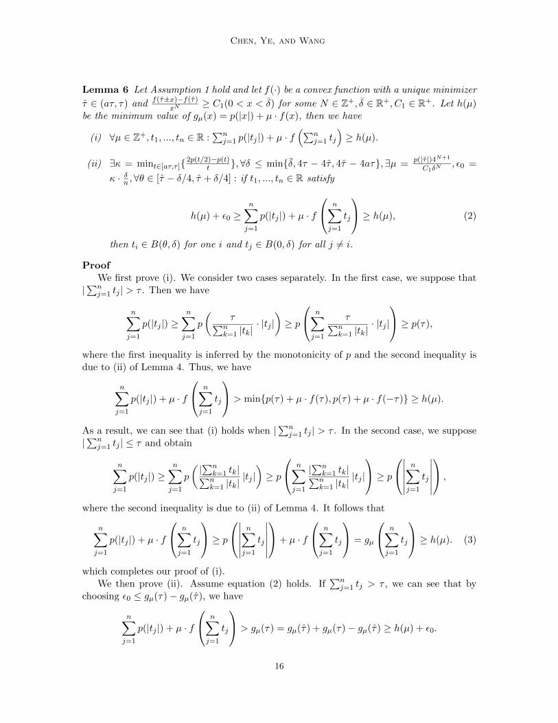
Lemma 5 Let Assumption 1 hold. Let f(·) be a convex function with a unique minimizer
τ ∈ (aτ, τ) and f(τ±x)−f(τ)xN
≥ C(0 < x < δ) for some N ∈ Z+, δ ∈ R+, C ∈ R+. Define
gµ(t) = p(|t|) + µ · f(t),
where µ > 0. Let h(µ) be the minimum value of gµ(·). We have ∀δ < δ, µδ >p(|τ |)2NCδN
, ∃ε0 =
µδ · C ·(δ2
)N − p(|τ |): if t satisfies h(µδ) + ε0 ≥ gµδ(t) ≥ h(µδ), then t ∈ [τ − δ/2, τ + δ/2].
Proof First, we can see that when t > τ + δ/2, we have
κ · δn ,∀θ ∈ [τ − δ/4, τ + δ/4] : if t1, ..., tn ∈ R satisfy
h(µ) + ε0 ≥n∑j=1
p(|tj |) + µ · f
n∑j=1
tj
≥ h(µ), (2)
then ti ∈ B(θ, δ) for one i and tj ∈ B(0, δ) for all j 6= i.
ProofWe first prove (i). We consider two cases separately. In the first case, we suppose that
|∑n
j=1 tj | > τ . Then we have
n∑j=1
p(|tj |) ≥n∑j=1
p
(τ∑n
k=1 |tk|· |tj |
)≥ p
n∑j=1
τ∑nk=1 |tk|
· |tj |
≥ p(τ),
where the first inequality is inferred by the monotonicity of p and the second inequality isdue to (ii) of Lemma 4. Thus, we have
n∑j=1
p(|tj |) + µ · f
n∑j=1
tj
> minp(τ) + µ · f(τ), p(τ) + µ · f(−τ) ≥ h(µ).
As a result, we can see that (i) holds when |∑n
j=1 tj | > τ . In the second case, we suppose|∑n
j=1 tj | ≤ τ and obtain
n∑j=1
p(|tj |) ≥n∑j=1
p
(|∑n
k=1 tk|∑nk=1 |tk|
|tj |)≥ p
n∑j=1
|∑n
k=1 tk|∑nk=1 |tk|
|tj |
≥ p∣∣∣∣∣∣
n∑j=1
tj
∣∣∣∣∣∣ ,
where the second inequality is due to (ii) of Lemma 4. It follows that
n∑j=1
p(|tj |) + µ · f
n∑j=1
tj
≥ p∣∣∣∣∣∣
n∑j=1
tj
∣∣∣∣∣∣+ µ · f
n∑j=1
tj
= gµ
n∑j=1
tj
≥ h(µ). (3)
which completes our proof of (i).We then prove (ii). Assume equation (2) holds. If
∑nj=1 tj > τ , we can see that by
choosing ε0 ≤ gµ(τ)− gµ(τ), we have
n∑j=1
p(|tj |) + µ · f
n∑j=1
tj
> gµ(τ) = gµ(τ) + gµ(τ)− gµ(τ) ≥ h(µ) + ε0.
16
Hardness for Sparse Optimization
We will show later that our choice of ε0 is indeed smaller than gµ(τ) − gµ(τ). We willalso show later that equation (2) cannot hold when
∑nj=1 tj < −τ under our choice of
parameters. Thus, if equation (2) holds, then |∑n
j=1 tj | ≤ τ , which implies that
p
∣∣∣∣∣∣n∑j=1
tj
∣∣∣∣∣∣+ µ · f
n∑j=1
tj
≤ h(µ) + ε0, (4)
by equation (2) and the first inequality of (3), and
n∑j=1
p(|tj |) ≤ p
∣∣∣∣∣∣n∑j=1
tj
∣∣∣∣∣∣+ ε0, (5)
due to equation (2) and equation (3). Note that we just need to prove the case whenδ is sufficiently small. Thus, we assume in the following paper that δ is smaller thanδ, 4τ − 4τ , 4τ − 4aτ .
Consider the case when equation (4) holds. By Lemma 6, if we choose µ = p(|τ |)4N+1
CδNand
ε1 = 3p(|τ |), then all of the points t such that h(µ)+ε1 ≥ gµ(t) ≥ h(µ) lie in [τ−δ/4, τ+δ/4].Thus, we have
∑nj=1 tj ∈ [aτ, τ ] and
∑nj=1 tj ∈ B(θ, δ2) for all θ ∈ [τ − δ/4, τ + δ/4]. Note
that gµ(t) is non-increasing when t < 0, meaning that equation (2) cannot hold under ourchoice of ε1 when
∑nj=1 tj ≤ −τ .
On the other hand, if equation (2) holds, equation (5) should also hold. By (iv) of Lemma4, for the same δ, ∃ε2 = mint∈[aτ,τ ](k1(t) − k2(t)) · δ
2n−2 , there is at most one i such that
ti 6∈ B(0, δ2n−2). As
∑nj=1 tj ∈ B(θ, δ2), we have ti ∈ B(θ, δ) for all i = 1, · · · , n. Observe
that gµ(τ) − gµ(τ) is always larger than ε1. Also, ε1 > ε2 if δ is sufficiently small. There-
j=1 ti), then ti ∈ B(θ, δ) for some i whiletj ∈ B(0, δ) for all j 6= i.
6.2. Proof of Theorem 1
Now we are ready to prove Theorem 1.Proof Suppose that we are given the input to the 3-partition problem, i.e., 3m positiveintegers s1, ..., s3m. Assume without loss of generality that all si’s are upper bounded bysome polynomial function M(m). This restriction on the input space does not weaken ourresult, because the 3-partition problem is strongly NP-hard.
In what follows, we construct a reduction from the 3-partition problem to Problem 1. Weassume without loss of generality that 1
4m
∑3mj=1 sj < si <
12m
∑3mj=1 sj for all i = 1, . . . , n.
Such condition can always be satisfied by adding a sufficiently large integer to all si’s.Step 1: The Reduction. The reduction is developed through the following steps.
1. For the interval [aτ, τ ], we choose b1ik1i=1 such that `1(y) = 1λ
∑k1i=1 `(y, b1i) satisfies
Assumption 1 with constants C,N, δ and has a unique minimizer τ inside the interval(aτ, τ). Let κ = mint∈[aτ,τ ]
2p(t/2)−p(t)t . Let δ ≤ aτ
9m·M(m) , δ, 4τ − 4τ , 4τ − 4aτ,
17
Chen, Ye, and Wang
µ ≥ p(|τ |)4N+1
C1δNand ε = κ · δ
3m such that Lemma 6 is satisfied. Note that ε ≥ C3m2·M(m)
for some constant C3 by our construction.
2. For the µ and ε chosen in the previous step, all the minimizers of gµ(x) = p(|x|) + µ ·`1(x) lie in [τ−δ/4, τ+δ/4] by Lemma 6. By the Lipschitz continuity of p(|x|), f(x) andthus gµ(x) on [aτ, τ ], there exists δε = ε
6mK (K is the Lipschitz constant) such that wecan find in polynomial time an interval [θ1, θ2] where θ2−θ1 = δε and gµ(x)−gµ(t∗) <ε
6m for x ∈ [θ1, θ2]. This interval can be find in polynomial time as gµ(x) is Lipschitzcontinuous.
3. By Assumption 2, for the interval [θ1, θ2], we choose b2ik2i=1 to construct a lossfunction `2 : R 7→ R in polynomial time with regard to 1/δε such that `2(y) =1λ
∑k2i=1 `(y, b2i) has a unique minimizer at t ∈ [θ1, θ2]. We choose
ν =⌈ε/max
(`2(t+ 2δm)− `2(t), `2(t− 2δm)− `2(t)
)⌉+ 1,
and construct function f : R3m×m 7→ R where
f(x) = λ ·3m∑i=1
m∑j=1
p (|xij |) + λµ ·3m∑i=1
`1
m∑j=1
xij
+ λν ·m∑j=1
`2
(3m∑i
si∑3mi′=1 si′/m
xij
).
(6)
Note that by (iii) of Assumption 2, ν is polynomial in max(d 1δεe, dθ2e). In the rest
of the paper, we ignore the dθ2e term in the bound as it can be upperbounded by τ ,which can be taken as a constant in the reduction.
4. Let Φ1 = 3m · p(|t|) + µ · 3m · `1(t)− ε2 and Φ2 = ν ·m · `2(t). We claim that
(i) If there exists z such that
Φ1 + Φ2 + ε ≥ 1
λf(z) ≥ Φ1 + Φ2,
then we obtain a feasible assignment for the 3-partition problem as follows: Ifzij ∈ B(t, δ), we assign number i to subset j.
(ii) If the 3-partition problem has a solution, we have 1λ minx f(x) ≤ Φ1 + Φ2 + ε
2 .
5. Choose r =
⌈(2(3m·λ·µ·k1+m·λ·ν·k2)c1 (3m2)
c2
ε/κ
)1/(1−c1−c2)⌉
where c1 and c2 are two arbi-
trary constants that c1 + c2 < 1. Construct the following instance of Problem 1:
minx(1),··· ,x(r)∈R3m×m
r∑q=1
f(x(q)) = minx(1),··· ,x(r)∈R3m×m
λ ·r∑q=1
3m∑i=1
m∑j=1
p(|x(q)ij |)+
λµr∑q=1
3m∑i=1
k1∑t=1
`
m∑j=1
x(q)ij , b1t
+ λνr∑q=1
m∑j=1
k2∑t=1
`
(3m∑i=1
si∑3mi′=1 si′/m
x(q)ij , b2t
),
(7)
18
Hardness for Sparse Optimization
where the input data are coefficients of x and the values b11, . . . , b1t, b21, . . . , b2t. Thevariable dimension d is r ·3m2 and the sample size n is λ ·µ · r ·3m ·k1 +λ ·ν · r ·m ·k2.The input size is polynomial with respect to m. Our choice of r is the solution toεr = 2κnc1dc2 where κ = mint∈[aτ,τ ]
2p(t/2)−p(t)t .
The parameters µ, ν, δ, r, d are bounded by polynomial functions of m. Computingtheir values also takes polynomial time. The parameter k1 and k2 is a constantdetermined by the loss function ` and is not related to m. As a result, the reductionis polynomial.
6. Let z(1), · · · z(r) ∈ R3m×m be a λ ·κ ·nc1dc2-optimal solution to problem (13) such that∑ri=1 f(z(i)) ≤ minx(1),··· ,x(r)
∑ri=1 f(x(i)) + λ · κ · nc1dc2 . We claim that
(iii) If the approximate solution z(1), · · · z(r) satisfies
1
λ
r∑i=1
f(z(i)) ≤ rΦ1 + rΦ2 + 2κnc1dc2 , (8)
we can choose one z(i) such that Φ1 + Φ2 + ε ≥ 1λf(z(i)) ≥ Φ1 + Φ2 and obtain
a feasible assignment: If z(i)ij ∈ B(t, δ), we assign number i to subset j. If the
λ · κ · nc1dc2-optimal solution z(1), · · · z(r) does not satisfy (8), the 3-partitionproblem has no feasible solution.
We have constructed a polynomial reduction from the 3-partition problem to finding anλ ·κ ·nc1dc2-optimal solution to problem (13). In what follows, we prove that the reductionworks.
Step 2: Proof of Claim (i). We begin with the proof (i). By our choice of µ and Lemma6(i), we can see that for all x ∈ R3m×m,
3m∑i=1
m∑j=1
p(|xij |) + µ ·3m∑i=1
`1
m∑j=1
xij
≥ 3m · p(|t∗|) + µ · 3m · `1(t∗) ≥ Φ1,
where the last inequality is due to that gµ(t)− gµ(t∗) < ε6m . By the fact t = argmint`2(t),
we have for all x ∈ R3m×m that
ν ·m∑j=1
h
(3m∑i=1
si∑3mi′=1 si′/m
xij
)≥ ν ·m · `2(t) = Φ2.
Thus we always have minz1λf(z) ≥ Φ1 + Φ2. Now if there exists z such that Φ1 + Φ2 + ε ≥
1λf(z) ≥ Φ1 + Φ2, we must have
Φ1 + ε ≥3m∑i=1
m∑j=1
p(|zij |) + µ ·3m∑i=1
h
m∑j=1
zij
≥ Φ1, (9)
and
Φ2 + ε ≥ ν ·m∑j=1
h
(3m∑i=1
si∑3mi′=1 si′/m
zij
)≥ Φ2. (10)
19
Chen, Ye, and Wang
In order for equation (9) to hold, we have that for all i,
p(|t|) + µ · `1(t) +ε
2≥
m∑j=1
p(|zij |) + µ · `1
m∑j=1
zij
≥ p(|t∗|) + µ · `1(t∗).
Consider an arbitrary i. By Lemma 6(ii) and gµ(t) − gµ(t∗) < ε6m , we have zij ∈ B(t, δ)
for one j while zik = 0 for all k 6= j. If zij ∈ B(t, δ), we assign number i to subset j.As δ < aτ/2 ≤ t/2, B(t, δ) and B(0, δ) are not overlapping. Thus each number index i isassigned to exactly one subset index j. Therefore the assignment is feasible.
We claim that every subset sum must equal to∑3m
i=1 si/m. Assume that the jth subsetsum is greater than or equal to
∑3mi=1 si/m + 1. Let Ij = i | zij ∈ B(t, δ). Thus,∑
i∈Ij si ≥∑3m
i=1 si/m+ 1. As a result, we have
3m∑i=1
si∑3mi′=1 si′/m
zij ≥∑i∈I1
si∑3mi′=1 si′/m
(t− δ) +∑i∈I2
si∑3mi′=1 si′/m
(−δ)
≥∑3m
i=1 si/m+ 1∑3mi=1 si/m
t− δm = t+t∑3m
i=1 si/m− δm.
Because si ≤M(m) for all i and δ = aτ9m·M(m) , we have
t∑3mi=1 si/m
− δm ≥ aτ
3m ·M(n)m− δm = 2δm > 0.
Since h is a convex function with minimizer y∗, we apply the preceding inequalities andfurther obtain
`2
(3m∑i=1
si∑3mi′=1 si′/m
zij
)≥ `2(t+ 2δm).
By our construction of ν and Assumption 1(iii), we further have
ν ·
(`2
(3m∑i=1
si∑3mi′=1 si′/m
zij
)− `2(t)
)≥ ν ·
(`2(t+ 2δm)− `2(t)
)> ε. (11)
However, in order for equation (10) to hold, we have that for all j,
ν · `2(t) + ε ≥ ν · `2
(3m∑i=1
si∑3mi′=1 si′/m
zij
)≥ ν · `2(t),
yielding a contradiction to (11). We could prove similarly that it is not possible for anysubset sum to be strictly smaller than 1
m
∑3mi=1 si. Therefore, the sum of every subset equals
to∑3m
i=1 si/m. Finally, using the assumption that 14m
∑3mi=1 si < si <
12m
∑3mi=1 si, each
subset has exactly three components. Therefore the assignment is indeed a solution to the3-partition problem.
Step 3: Proof of Claim (ii). Suppose we have a solution to the 3-partition problem.Now we construct z to the optimization problem such that f(z) ≤ Φ1 + Φ2 + ε
2 . For all
20
Hardness for Sparse Optimization
1 ≤ i ≤ 3m, if number i is assigned to subset j, let zij = t and zik = 0 for all k 6= j. Wecan easily verify that
3m∑i=1
m∑j=1
p (|zij |) + µ ·3m∑i=1
`1
m∑j=1
zij
= 3m ·(p(t) + µ · `1(t)
)= Φ1 +
ε
2,
Also, we have
ν ·m∑j=1
`2
(3m∑i=1
si∑3mi′=1 si′/m
zij
)= ν ·m · `2(t) = Φ2.
Therefore,1
λf(z) ≤ Φ1 + Φ2 +
ε
2. (12)
which completes the proof of (ii).
Step 4: Proof of Claim (iii). Suppose that the λ ·κ ·nc1dc2-optimal solution satisfies (8),i.e., 1
λ
∑ri=1 f(z(i)) ≤ rΦ1 + rΦ2 + 2κnc1dc2 . It follows that there exists at least one term
z(i) such that1
λf(z(i)) ≤ Φ1 + Φ2 +
2κnc1dc2
r≤ Φ1 + Φ2 + ε.
where the second inequality equality uses εr = 2κnc1dc2 . Therefore, by claim (ii), we canfind a solution to the 3-partition problem.
Suppose that the 3-partition problem has a solution. By claim (ii), there exists z suchthat 1
λf(z) ≤ Φ1 + Φ2 + ε2 . Thus we have
minx(1),··· ,x(r)
1
λ
r∑i=1
f(x(i)) ≤ r
λf(z) ≤ rΦ1 + rΦ2 + κnc1dc2 .
Thus if z(1), · · · z(r) is a λ · κ · nc1dc2-optimal solution to (13), we have
1
λ
r∑i=1
f(z(i)) ≤ minx(1),··· ,x(r)
1
λ
r∑i=1
f(x(i)) + κnc1dc2 ≤ rΦ1 + rΦ2 + 2κnc1dc2
implying that the relation (8) must hold. If (8) is not satisfied, the 3-partition problem hasno solution.
Remark. When the loss function is L2 loss, we can move λµ and λν of equation (13) intothe loss. Specifically, we have
minx(1),··· ,x(r)∈R3m×m
r∑q=1
f(x(q)) = minx(1),··· ,x(r)∈R3m×m
λ ·r∑q=1
3m∑i=1
m∑j=1
p(|x(q)ij |)+
r∑q=1
3m∑i=1
m∑j=1
√λµx
(q)ij −
√λµb1
2
+r∑q=1
m∑j=1
(3m∑i=1
√λνsi∑3m
i′=1 si′/mx
(q)ij −
√λνb2
)2
,
(13)
21
Chen, Ye, and Wang
where µ, ν is chosen such that√λµ,√λν are rational numbers. In this case, the variable
dimension is r · 3m2 and the sample size n is 4r · m. Our choice of r is the solution to
εr = 2κnc1dc2 which is r =
⌈(2(4m)c1 (3m2)
c2
ε/κ
)1/(1−c1−c2)⌉
. The value of r doesn’t depend on
λ and p, which means that we can plug in any λ, p and the reduction is still polynomial inm. It means that for any choice of λ and p, it is strongly NP hard to find a λκnc1dc2-optimalsolution.
6.3. Proof of Theorem 2
Next we study the complexity of Problem 2. The proof uses a basic duality between Problem1 and Problem 2.
Proof We will use a reduction from the 3-partition problem to prove the theorem. Thereduction is developed through the following steps. We first constructed a polynomialreduction from the 3-partition problem to finding an approximate solution to Problem 2.We then prove that the reduction works.
1. Given the input to the 3-partition problem, we conduct the first three steps of thereduction in Theorem 1 to compute µ, ν, t and ε with λ = 1. The nuance is that we pickδε = ε
12mK in step 2 so that gµ(t)−gµ(t∗) ≤ ε12m where gµ(x) = p(|x|)+µ·`1(x). Denote
f(x) = µ ·∑3m
i=1
∑k1t=1 `
(∑mj=1 xij , b1t
)+ ν ·
∑mj=1
∑k2t=1 `
(∑3mi=1
si∑3mi′=1 si′/m
xij , b2t
)and q(x) =
∑3mi=1
∑mj=1 p (|xij |).
2. Choose r =
⌈(4(3m·µ·k1+m·ν·k2)c1 (3m2)
c2
ε/κ
)1/(1−c1−c2)⌉
where c1 and c2 are two arbitrary
constants that c1 + c2 < 1. Note that κnc1dc2 = εr4 by our choice of r. Construct the
following instance of Problem 2:
minx(1),x(2),...,x(r)∈R3m×m
r∑i=1
f(x(i)) s.t.r∑i=1
q(x(i)) ≤ K, (14)
where K ∈ [3m · r · p(t), 3m · r · p(t) + εr/4). The coding size of K is bounded bya polynomial function of m because εr/4 and 3m · r · p(t) are both bounded by apolynomial functions of n. Denote the minimizer of the minimization problem (14)
to be x(1)
K, · · ·x(r)
K.
3. Let Φ1 = 3m · p(|t|) + µ · 3m · `1(t) − ε4 and Φ2 = ν ·m · `2(t). We claim that if the
3-partition problem has a solution, then
(i)∑r
i=1 f(x(i)
K) +
∑ri=1 q(x
(i)
K) ≤ rΦ1 + rΦ2 + εr
2 .
(ii)∑r
i=1 q(x(i)
K) ≥ 3m · r · p(t)− εr/4.
4. Suppose we have approximate solutions satisfying∑r
i=1 f(x(i)
K+κnc1dc2) ≤
∑ri=1 f(x
(i)
K),
we claim that
22
Hardness for Sparse Optimization
(iii) If the approximate solutions satisfy
r∑i=1
f(x(i)
K+κnc1dc2) +
r∑i=1
q(x(i)
K+κnc1dc2) ≤ rΦ1 + rΦ2 + 4κnc1dc2 , (15)
we can choose one index k such that Φ1 + Φ2 + ε ≥ f(x(k)
K+κnc1dc2) ≥ Φ1 + Φ2
and obtain a feasible assignment: If(x
(k)
K+κnc1dc2
)ij∈ B(t, δ), we assign number
i to subset j. If the approximate solutions do not satisfy (15), the 3-partitionproblem has no feasible solution.
We begin with the proof of (i). By the condition that the 3-partition problem has asolution, we construct x∗ ∈ R3m×m as follows. If number i is assigned to subset j, let x∗ij = t
and x∗ik = 0 otherwise. We can see that x(1) = · · · = x(r) = x∗ satisfy the constraint of (14)
with sparsity level K and∑r
i=1 q(x(i)
K) ≤ 3m · r · p(t) + εr/4. Thus,
r∑i=1
f(x(i)
K) +
r∑i=1
q(x(i)
K) ≤ r · f(x∗) + 3m · r · p(t) +
εr
4= r · 3m · gµ(t) + rΦ2 +
εr
4
= r · 3m ·(gµ(t)− ε
12m
)+ rΦ2 +
εr
2= rΦ1 + rΦ2 +
εr
2,
(16)
where gµ(x) = p(|x|) + µ · `1(x). To prove (ii), we just need to notice that if∑r
i=1 q(x(i)
K) <
3m · r · p(t) − εr/4, we would have∑r
i=1 f(x(i)
K) +
∑ri=1 q(x
(i)
K) < rΦ1 + rΦ2 by the same
reasoning of equation (16), yielding a contradiction as∑r
i=1 f(x(i)
K)+∑r
i=1 q(x(i)
K) will always
be greater than or equal to rΦ1 + rΦ2.Now we prove (iii). To prove the first half of the claim, we only need to use 4κnc1dc2 = rε
and apply the proof of Theorem 1 to get the result. To prove the second half of the claim,
assume that we have an algorithm that outputs xK+κnc1dc2 satisfying∑r
i=1 f(x(i)
K+κnc1dc2) ≤∑r
i=1 f(x(i)
K). Suppose that the 3-partition problem has a solution. Then we have
r∑i=1
f(x(i)
K+κnc1dc2) +
r∑i=1
q(x(i)
K+κnc1dc2) ≤
r∑i=1
f(x(i)
K) +
r∑i=1
q(x(i)
K) +
εr
2≤ rΦ1 + rΦ2 + εr,
where the first inequality is due to (ii) and the second inequality is due to (i). It meansthat the approximate solutions satisfy (15). To this point, we have finished the proof ofTheorem 2.
Remark. Note that K is the input of Problem 2, which means that for all ` and p, weonly need to find a K that makes Problem 2 hard to solve. A natural question to ask iswhether or not K could be the parameter of Problem 2 such that the hardness result stillholds. Unfortunately, we have the following counterexample. Assume p is L0 norm andK = 1. Then the constraint is
∑dj=1 L0(xj) ≤ 1, which means that there is at most one
component of x that is not equal to 0. In this case, we could solve the optimization problemin polynomial time by searching for the nonzero component of x.
23
Chen, Ye, and Wang
6.4. Proof of Theorem 3
Using a similar argument, we can prove the last part of our main result.Proof The proof is analogous to the proof of Theorem 2. We will use a reduction from the3-partition problem to prove the theorem. The reduction is developed through the followingsteps.
1. Given the input to the 3-partition problem, we conduct the first reduction step of The-
orem 2 to compute µ, ν, t and ε with λ = 1. Let f(x) = µ·∑3m
i=1
∑k1t=1 `
(∑mj=1 xij , b1t
)+
ν ·∑m
j=1
∑k2t=1 `
(∑3mi=1
si∑3mi′=1 si′/m
xij , b2t
)and q(x) =
∑3mi=1
∑mj=1 p (|xij |).
2. Choose r =
⌈(4(3m·µ·k1+m·ν·k2)c1 (3m2)
c2
ε/κ
)1/(1−c1−c2)⌉
where c1 and c2 are two arbitrary
constants that c1 + c2 < 1. Note that κnc1dc2 = εr4 by our choice of r. Construct the
following instance of Problem 3:
minx(1),x(2),...,x(r)∈R3m×m
r∑i=1
q(x(i)) s.t.
r∑i=1
f(x(i)) ≤ η, (17)
where η ∈ [µ · 3m · `1(t) + ν · m · `2(t), µ · 3m · `1(t) + ν · m · `2(t) + εr/4). Notethat the parameters µ, ν, δ,m, r, d and η are bounded by polynomial functions of n.Computing their values also takes polynomial time. Given the sparsity level η, denote
the minimizer of (17) to be x(1)η , · · ·x(r)
η .
3. Let Φ1 = 3m · p(|t|) + µ · 3m · `1(t) − ε4 and Φ2 = ν ·m · `2(t). We claim that if the
4. Suppose we have an approximate solution satisfying∑r
i=1 f(x(i)η+κnc1dc2 ) ≤
∑ri=1 f(x
(i)η ),
we claim that
(iii) If the approximate solution satisfies
r∑i=1
f(x(i)η+κnc1dc2 ) +
r∑i=1
q(x(i)η+κnc1dc2 ) ≤ rΦ1 + rΦ2 + 4κnc1dc2 , (18)
we can choose the index k such that Φ1 + Φ2 + ε ≥ f(x(k)η+κnc1dc2 ) ≥ Φ1 + Φ2
and obtain a feasible assignment: If(x
(k)η+κnc1dc2
)ij∈ B(t, δ), we assign number
i to subset j. If the approximate solutions do not satisfy (18), the 3-partitionproblem has no feasible solution.
We have constructed a polynomial reduction from the 3-partition problem to finding anapproximate solution to Problem 3. We then prove that the reduction works. We begin
24
Hardness for Sparse Optimization
with the proof of (i). By the condition that the 3-partition problem has a solution, weconstruct x∗ ∈ R3m×m as follows. If number i is assigned to subset j, let x∗ij = t and
x∗ik = 0 otherwise. We can see that x(1) = · · · = x(r) = x∗ satisfy the constraint of (14)
where gµ(x) = p(|x|) + µ · `1(x) and the last inequality is due to the choice of t in step 1 ofthe reduction.
To prove (ii), we just need to notice that if∑r
i=1 f(x(i)η ) ≤ µ·3m·`1(t)+ν ·m·`2(t)−εr/4,
we would have∑r
i=1 f(x(i)η ) +
∑ri=1 q(x
(i)η ) < rΦ1 + rΦ2 by the same reasoning of equation
(16), yielding a contradiction as∑r
i=1 f(x(i)η ) +
∑ri=1 q(x
(i)η ) will always be greater than or
equal to rΦ1 + rΦ2.Now we prove (iii). To prove the first half of the claim, we only need to use 4κnc1dc2 = rε
and apply the proof of Theorem 1 to get the result. To prove the second half of the
claim, assume that we have an algorithm that outputs xη satisfying∑r
i=1 f(x(i)η+κnc1dc2 ) ≤∑r
i=1 f(x(i)η ). Suppose that the 3-partition problem has a solution. Replacing η by η gives
usr∑i=1
f(x(i)η+κnc1dc2 ) +
r∑i=1
q(x(i)η+κnc1dc2 ) ≤
r∑i=1
f(x(i)η ) +
r∑i=1
q(x(i)η ) +
εr
2≤ rΦ1 + rΦ2 + εr,
where the first inequality is due to (ii) and the second inequality is due to (i). It meansthat the approximate solutions satisfy (18). To this point, we have finished the proof ofTheorem 3.
References
E. Amaldi and V. Kann. On the approximability of minimizing nonzero variables or unsat-isfied relations in linear systems. Theoretical Computer Science, 209(1):237–260, 1998.
A. Antoniadis and J. Fan. Regularization of wavelet approximations. Journal of the Amer-ican Statistical Association, 96(455):939–967, 2001.
S. Arora, L. Babai, J. Stern, and Z. Sweedy. The hardness of approximate optima inlattices, codes, and systems of linear equations. In Foundations of Computer Science,1993. Proceedings., 34th Annual Symposium on, pages 724–733. IEEE, 1993.
W. Bian and X. Chen. Optimality conditions and complexity for Non-Lipschitz constrainedoptimization problems. Preprint, 2014.
A. M. Bruckstein, D. L. Donoho, and M. Elad. From sparse solutions of systems of equationsto sparse modeling of signals and images. SIAM review, 51(1):34–81, 2009.
25
Chen, Ye, and Wang
A. C. Cameron and P. K. Trivedi. Regression analysis of count data, volume 53. Cambridgeuniversity press, 2013.
E. Candes, M. Wakin, and S. Boyd. Enhancing sparsity by reweighted L1 minimization.Journal of Fourier Analysis and Applications, 14(5-6):877–905, 2008.
R. Chartrand. Exact reconstruction of sparse signals via nonconvex minimization. SignalProcessing Letters, IEEE, 14(10):707–710, 2007.
X. Chen, D. Ge, Z. Wang, and Y. Ye. Complexity of unconstrained L2 − Lp minimization.Mathematical Programming, 143(1-2):371–383, 2014.
Y. Chen and M. Wang. Hardness of approximation for sparse optimization with L0 norm.Technical Report, 2016.
Y. Chen, D. Ge, M. Wang, Z. Wang, Y. Ye, and H. Yin. Strong NP-hardness for sparseoptimization with concave penalty functions. ICML, 2017.
G. Davis, S. Mallat, and M. Avellaneda. Adaptive greedy approximations. Constructiveapproximation, 13(1):57–98, 1997.
J. Fan and R. Li. Variable selection via nonconcave penalized likelihood and its oracleproperties. Journal of the American Statistical Association, 96(456):1348–1360, 2001.
J. Fan and J. Lv. A selective overview of variable selection in high dimensional featurespace. Statistica Sinica, 20(1):101–148, 2010.
J. Fan, L. Xue, and H. Zou. Strong oracle optimality of folded concave penalized estimation.The Annals of Statistics, 42(3):819–849, 2014.
J. Fan, H. Liu, Q. Sun, and T. Zhang. TAC for sparse learning: Simultaneous control ofalgorithmic complexity and statistical error. arXiv preprint arXiv:1507.01037, 2015.
E. X. Fang, H. Liu, and M. Wang. Blessing of massive scale: Spatial graphical modelinference with a total cardinality constraint. working paper, 2015.
D. Foster, H. Karloff, and J. Thaler. Variable selection is hard. In COLT, pages 696–709,2015.
L. E. Frank and J. H. Friedman. A statistical view of some chemometrics regression tools.Technometrics, 35(2):109–135, 1993.
M. R. Garey and D. S. Johnson. “Strong” NP-Completeness results: Motivation, examples,and implications. Journal of the ACM, 25(3):499–508, 1978.
D. Ge, Z. Wang, Y. Ye, and H. Yin. Strong NP-hardness result for regularized Lq-minimization problems with concave penalty functions. arXiv preprint arXiv:1501.00622,2015.
P. J. Huber. Robust estimation of a location parameter. The Annals of MathematicalStatistics, 35(1):73–101, 1964.
26
Hardness for Sparse Optimization
X. Huo and J. Chen. Complexity of penalized likelihood estimation. Journal of StatisticalComputation and Simulation, 80(7):747–759, 2010.
P.-L. Loh and M. J. Wainwright. Regularized M-estimators with nonconvexity: Statisticaland algorithmic theory for local optima. In Advances in Neural Information ProcessingSystems, pages 476–484, 2013.
J. Lv and Y. Fan. A unified approach to model selection and sparse recovery using regu-larized least squares. The Annals of Statistics, 37(6A):3498–3528, 2009.
P. McCullagh. Generalized linear models. European Journal of Operational Research, 16(3):285–292, 1984.
B. K. Natarajan. Sparse approximate solutions to linear systems. SIAM journal on com-puting, 24(2):227–234, 1995.
X. Shen, W. Pan, and Y. Zhu. Likelihood-based selection and sharp parameter estimation.Journal of the American Statistical Association, 107(497):223–232, 2012.
R. Tibshirani. Regression shrinkage and selection via the lasso. Journal of the RoyalStatistical Society. Series B (Methodological), pages 267–288, 1996.
V. V. Vazirani. Approximation Algorithms. Springer Science & Business Media, 2001.
L. Xue, H. Zou, T. Cai, et al. Nonconcave penalized composite conditional likelihoodestimation of sparse ising models. The Annals of Statistics, 40(3):1403–1429, 2012.
C.-H. Zhang. Nearly unbiased variable selection under minimax concave penalty. TheAnnals of Statistics, 38(2):894–942, 2010a.
T. Zhang. Analysis of multi-stage convex relaxation for sparse regularization. Journal ofMachine Learning Research, 11:1081–1107, 2010b.
Y. Zhang, M. J. Wainwright, and M. I. Jordan. Lower bounds on the performance ofpolynomial-time algorithms for sparse linear regression. In COLT, 2014.