Approximations of the lattice dynamics

Approximations of the lattice dynamics

APPROXIMATIONS OF THE LATTICE DYNAMICS

BY

AMJAD KHAN, M.Phill.

a thesis

submitted to the department of mathematics & statistics

and the school of graduate studies

of mcmaster university

in partial fulfilment of the requirements

for the degree of

Master of Science

c© Copyright by Amjad Khan, April, 2015

All Rights Reserved

Master of Science (2015) McMaster University

(Mathematics & Statistics) Hamilton, Ontario, Canada

TITLE: Approximations of the lattice dynamics

AUTHOR: Amjad Khan

M.Phill., (Mathematics)

National University of Sciences & Technology (NUST),

Islamabad, Pakistan.

SUPERVISOR: Dr. Dmitry Pelinovsky

NUMBER OF PAGES: viii, 51

ii

To my family.

Abstract

This investigation is devoted to the study of the Fermi-Pasta-Ulam (FPU) lattice dynamics.Approximations of the FPU lattice dynamics have been an old subject, it is believed thatthe stability of the FPU traveling waves depends on the stability of the KDV solitary waves.The key question is: Are the traveling waves of the FPU lattice stable if the traveling waves

of KDV type equation are stable?.

We consider the FPU lattice with the nonlinear potential which leads to the generalizedKorteweg-de Vries (gKDV) equation, which is known to have orbitally stable traveling wavesin a subcritical case and orbitally unstable traveling waves in critical and supercritical cases.In order to pursue the question asked above, we use the energy method.

We establish that the Hs(R) norm of the solution of the gKDV equation is bounded bya time-independent constant in the subcritical case, whereas the Hs(R) norm grows at mostexponentially in time in the critical and supercritical cases. With the help of these results,we extend the time scale for the approximation of the traveling waves of the FPU latticeby the traveling waves of the gKDV equation logarithmically in the subcritical case. In thecritical and supercritical cases, we extend the time scale by a double-logarithmic factor.

Our results show that the traveling waves of the FPU lattice are stable if the solitarywaves of the gKDV equation are stable in the subcritical case. On the other hand, in thecritical and supercritical cases, our results are restricted to small-norm initial data, whichexclude solitary waves.

iv

Acknowledgements

First and foremost, I would like to thank my supervisor, Dr. Dmitry Pelinovsky, for all of hissupport throughout this research endeavour and for having the con�dence to o�er me thisopportunity. His mentorship has allowed me to grow both academically and personally, andfor this I would like to extend my sincere gratitude. I very much look forward to our futurecollaboration! I would also like to thank the members of my examination committee, Dr.Bartosz Protas and Dr. Gail S. K. Wolkowicz, for all of their input and recommendationsabout my thesis. In addition, I would like to acknowledge the Mathematics and Statisticsdepartment at McMaster University which I consider to be a great work environment, full ofmany genuine and friendly people. Finally, I am deeply indebted to my family and friendsfor their continuous support.

v

Contents

Abstract iv

Acknowledgements v

1 Introduction 1

1.1 A one dimensional Fermi-Pasta-Ulam chain . . . . . . . . . . . . . . . . . . . 1

1.2 Some historical background . . . . . . . . . . . . . . . . . . . . . . . . . . . . 2

1.3 Formal derivation of the KDV type equation . . . . . . . . . . . . . . . . . . . 3

1.4 Problem statement and motivation . . . . . . . . . . . . . . . . . . . . . . . . 6

1.5 Organization of the Thesis . . . . . . . . . . . . . . . . . . . . . . . . . . . . . 8

2 Properties of the gKDV equation 10

2.1 Exact traveling wave solution to the gKDV equation . . . . . . . . . . . . . . 10

2.2 Global well posedness of the gKDV equation . . . . . . . . . . . . . . . . . . . 13

2.2.1 Global existence in H1(R) (p = 2, 3, 4, 5). . . . . . . . . . . . . . . . . 14

2.2.2 Integrable cases (p = 2, 3) . . . . . . . . . . . . . . . . . . . . . . . . . 18

2.2.3 Critical and supercritical cases (p ≥ 5) . . . . . . . . . . . . . . . . . . 21

3 Approximations of the Fermi-Pasta-Ulam lattice dynamics 27

3.1 Derivation of the gKDV equation and residual terms . . . . . . . . . . . . . . 31

3.2 Bounds on residual terms . . . . . . . . . . . . . . . . . . . . . . . . . . . . . 33

vi

3.3 Justi�cation of gKDV equation on the standard time scale . . . . . . . . . . . 37

3.4 Justi�cation of gKDV equation on the extended time scale . . . . . . . . . . . 39

4 Conclusion 46

vii

List of Figures

1.1 One dimensional spring mass system . . . . . . . . . . . . . . . . . . . . . . . 1

2.1 The solitary wave W for p = 2, 3, 4, 5, 6 and B = 0. . . . . . . . . . . . . . . . 13

viii

Chapter 1

Introduction

1.1 A one dimensional Fermi-Pasta-Ulam chain

To study the transfer of heat energy in solids, E. Fermi, J. Pasta, and S. Ulam carried out

a series of experiments at Los Alamos Laboratory in the middle of 1950s [1]. These exper-

iments are discussed in detail in subsequent publications [2, 3, 4]. The solid was modeled

by a one dimensional chain of particles of equal masses connected by nonlinear identical

springs (Figure 1.1). If the domain is unbounded, any particle can be selected as the ze-

roth particle, so that all other particles can be labeled with n ∈ Z. The equation of motion

governing the nth particle in the chain can be obtained by applying Newton's law of motion.

Figure 1.1: One dimensional spring mass system

Let us denote displacement produced in the nth particle by xn. The spring connecting

the nth and (n + 1)th particle is deformed by the displacement xn+1 − xn. Similarly, the

1

M.Sc. Thesis - Amjad Khan McMaster -Mathematics & Statistics

spring connecting the nth and (n−1)th particles is deformed by the displacement xn−xn−1.

Let V be the potential energy of each spring. The force exerted by each spring is −V ′ . Now

applying Newton's law of motion to the nth particle we get

xn = V ′(xn+1 − xn)− V ′(xn − xn−1), n ∈ Z. (1.1)

Let us now introduce variables for the relative displacement, un = xn+1 − xn, n ∈ Z.

Equations (1.1) become xn = V ′(un)−V ′(un−1), and xn+1 = V ′(un+1)−V ′(un). Subtracting

the former equation from the latter, we get

un = V ′(un+1)− 2V ′(un) + V ′(un−1), n ∈ Z. (1.2)

The lattice equation (1.2) is referred to as Fermi-Pasta-Ulam (FPU) lattice equation. The

sequence (un)n∈Z is a function of time t ∈ R, with values in RZ and the dot denotes the

time derivative.

1.2 Some historical background

In [1], E. Fermi, J. Pasta, and S. Ulam studied the heat conduction problem modeled by the

�nite spring-mass system (Figure 1.1). Fermi, Pasta and Ulam considered di�erent number

of masses in their experiments, e.g., 16, 32, 64. They were expecting that upon excitation

the nonlinear interactions would cause the equipartition of the energy. They carried out

computer simulations, which led to a completely di�erent outcome. The system did not

approach equipartition, rather the energy returned to the originally excited mode and a few

other nearby modes. This phenomenon is known as FPU recurrence.

2


The major development in the history of FPU system was made when N. J. Zabusky

and M. D. Kruskal in [2] approximated the FPU spring-mass system by the Korteweg�de

Vries (KDV) equation. They established a relation between the FPU recurrence and the

nondestructive collision of solitons of the KDV equation. The authors of [2] explained FPU

recurrence by decomposing the initial data into several solitons with di�erent velocities. The

lattice being of �nite length re�ects the solitons at the end points, which causes the solitons

to collide with each other. However, during the collision solitons preserve their shapes and

velocities. The authors of [2] conclude that at some later time, all the solitons arrive almost

in the same phase and almost reconstruct the initial state through the nonlinear interaction.

Not everyone was convinced with the computation of FPU [1], the popular conjecture

was that FPU had not run the simulations long enough and the time required to achieve

equipartition of energy may be too long to observe numerically. In 1972 Los Alamos physi-

cists J. L. Tuck and M. T. Menzel in [3] provided further insight into the FPU phenomenon

with numerical simulations that revealed recurrences on long time scales. A more detailed

overview of the FPU phenomenon is given by J. Ford in [4].

1.3 Formal derivation of the KDV type equation

For the class of an anharmonic potential, we will choose V (u) in the form

V (u) =1

2u2 +

ε2

p+ 1up+1, (1.3)

where ε is the strength of the anharmonicity and p ≥ 2, p ∈ N. The equation (1.2) can be

re-written as

un = un+1 − 2un + un−1 + ε2(upn+1 − 2upn + upn−1), n ∈ Z. (1.4)

3


The above FPU lattice (1.4) can be reduced to the generalized Koreweg-de Vries (gKDV)

equation by using the leading order solution

un(t) =W(ε(n− t), ε3t

)=W (ξ, τ) , ξ = ε(n− t), and τ = ε3t.

Using formal Taylor's series, we expand un+1 to get

un+1 = W(ε(n− t) + ε, ε3t

)=W (ξ + ε, τ)

= W + εWξ +ε2

2!Wξξ +

ε3

3!Wξξξ +

ε4

4!Wξξξξ +O(ε5), (1.5)

here partial derivatives are denoted by subscripts. Now using the Taylor's series expansion

for un−1 we obtain

un−1 = W(ε(n− t)− ε, ε3t

)=W (ξ − ε, τ)

= W − εWξ +ε2

2!Wξξ −

ε3

3!Wξξξ +

ε4

4!Wξξξξ −O(ε5). (1.6)

From (1.5) and (1.6) we obtain

un+1 − 2un + un−1 = ε2Wξξ +1

12ε4Wξξξξ +O(ε6) (1.7)

and

upn+1 − 2upn + upn−1 = ε2 (W p)ξξ +O(ε4). (1.8)

Next applying the chain rule to un =W (ξ, τ), where ξ = ε(n− t), τ = ε3t, we have

un =∂W

∂ξ

∂ξ

∂t+∂W

∂τ

∂τ

∂t= −εWξ + ε3Wτ

4


and

un = −ε(−εWξ + ε3Wτ

)ξ+ ε3

(−εWξ + ε3Wτ

)τ

= ε2Wξξ − 2 ε4Wξτ + ε6Wττ . (1.9)

Substituting (1.7), (1.8) and (1.9) in (1.4) we obtain

2 ε4Wξτ +1

12ε4Wξξξξ + ε4 (W p)ξξ +O(ε

6) = 0.

Comparing the coe�cients of ε4, we get at the leading order,

2Wξτ +1

12Wξξξξ + (W p)ξξ = 0. (1.10)

Integrating once with respect to ξ subject to the zero boundary conditions, we obtain

2Wτ +1

12Wξξξ + (W p)ξ = 0, ξ ∈ R. (1.11)

This equation (1.11) is called the generalized Korteweg�de Vries (gKDV) equation.

For p = 2, equation (1.11) reduces to the Korteweg�de Vries (KDV) equation derived

by Korteweg and de Vries [5] in the context of propagation of long waves in shallow water.

For p = 3, equation (1.11) reduces to the modi�ed Korteweg�de Vries (mKDV) equation.

The KDV and mKDV equations are studied extensively due to their relevance in a number

of physical systems. It was found that these models are integrable by the inverse scattering

transform method [6]. Equation (1.11) is called subcritical if 2 ≤ p ≤ 4, critical if p = 5 and

supercritical for p ≥ 6, with respect to how L2(R) changes under a dilation.

5


1.4 Problem statement and motivation

Justi�cation of the gKDV equation in the context of the FPU lattices has been a subject

of interest for many authors. G. Friesecke and R.L. Pego in the series of papers [7, 8, 9, 10]

justi�ed the KDV approximation for traveling waves and proved the nonlinear stability of

small amplitude solitary waves in generic FPU chains from analysis of the orbital and asymp-

totic stability of KDV solitons. T. Mizumachi [11, 12], A. Ho�man and C. E. Wayne [13],

and G. N. Benes, A. Ho�man and C. E. Wayne [14] extended these results to the proof of

asymptotic stability of several solitary waves in the FPU lattices. G. Schneider and C. E.

Wayne in [15] obtained the validity of the KDV equation for time-dependent solutions on

the time scale of O(ε−3). J. Gaison, and S. Moskow, and J.D. Wright, and Q. Zhang in [16]

generalized these results for polyatomic FPU lattices.

The approximation of the traveling waves in the FPU lattice by the KDV type equation

leads to a popular belief that The nonlinear stability of the FPU traveling waves resembles

the orbital stability of the KDV solitary waves. For the KDV equation, the positive traveling

waves are orbitally stable for all amplitudes and the FPU traveling waves are also stable

[7, 8, 9, 10]. On the other hand, there are some nonlinear potentials which may lead to the

KDV type equations whose traveling waves are not stable for all amplitudes. For example, if

we consider the nonlinear potential (1.3), we arrive at the generalized KDV equation (1.11),

which is known to have orbitally stable traveling waves for p = 2, 3, 4 (subcritical case) and

orbitally unstable traveling waves for p ≥ 5 (critical and supercritical case) [17]. This leads

to the question: Are the traveling waves of the FPU lattice (1.4) stable if the traveling waves

of the gKDV equation (1.11) are orbitally stable? This is the main question addressed in

this thesis.

Relevant results were obtained by E. Dumas and D. Pelinovsky in [18] on the validity of

6


the KDV type approximation for stability theory of traveling waves in FPU lattices. In [18]

an analytical technique was used to obtain the justi�cation of the log-KDV equation in the

context of FPU lattices. Nonlinear stability of all FPU traveling waves up to the time scale

of O(ε−3) was established, if the traveling waves satisfy the speci�c scaling leading to the

log-KDV approximation (see Theorem 2 in [18]). Theorem 3 in [18] showed that the non-

linear stability of the FPU traveling waves on the time scale of O(ε−3) may depend on the

orbital stability of the traveling waves in the KDV type equation. Authors of [18] say that

at �rst it appears that the results of Theorem 2 and Theorem 3 are in contradiction. They

further claim that no contradiction arises as a matter of fact, because the energy method

used in the proof of Theorems 2 and 3 gives the upper bound on the approximation errors

to be exponentially growing at the time scale of O(ε3). As a result, the unstable eigenvalues

of the linearized gKDV equation at the traveling waves lead to exponential divergence at

the time scale of O(ε3), which can not be detected by the approximation results provided

by Theorems 2 and 3.

The technique used in [18] is more general and is applicable to a large class of FPU

models, which results in the generalized KDV equation with possibly large-amplitude trav-

eling waves. One did not have to construct the two-dimensional manifold of traveling waves

or to use projections and modulation equations from the theory in [8, 9, 10]. The latter

theory gives a complete proof of nonlinear orbital stability of FPU traveling waves of small

amplitude, but it relies on the information about the spectral and asymptotic stability of

the KDV traveling waves, which is only available in the case of integrable KDV equation

(1.11) with p = 2. The result regarding the nonlinear stability of the FPU traveling waves

(Theorem 2 in [18]) does not depend on the nonlinear potential as long as some speci�c

scaling leading to the KDV type approximation is available.

7


1.5 Organization of the Thesis

We consider the nonlinear potential (1.3) and approximate the traveling waves of the FPU

lattice (1.4) by the traveling waves of the gKDV equation (1.11). Following the previous

work in [15, 18], we show that FPU traveling waves can be approximated by the gKDV

equation (1.11) up to the time scale O(ε3), even though the traveling waves of the gKDV

equation (1.11) are orbitally unstable if p ≥ 5.

We also give a partial answer to the question raised in the Section 1.4. We show that

the traveling waves of the FPU lattice (1.4) are stable up to an extended time scale for the

gKDV equation with p = 2, 3 (integrable subcritical cases) and for p ≥ 5 (critical and super-

critical cases), the latter results are proved under the small-norm assumption that exclude

solitary waves.

The thesis is organized as follow. In Chapter 2 we discuss some properties of the gKDV

equation, according to the following sections:

• In Section 2.1, the traveling solitary wave solution to the gKDV equation (1.11) is

derived.

• In Section 2.2, we discuss the local and global well posedness of the gKDV equa-

tion (1.11). The discussion of global existence is further divided into the following

subsections:

� In Subsection 2.2.1, globally well posedness is carried out for the subcritical and

critical gKDV equation (1.11) in H1(R).

� In Subsection 2.2.2, the integrable cases of the gKDV equation (1.11) are dis-

cussed. Using conserved quantities, it is shown that the solution is globally well

posed in Hs(R) and the upper bound on the Hs(R) norm of the solution does

8


not depend on time τ, for every s ∈ N.

� In Subsection 2.2.3, we review a result about the global well posedness of the

gKDV equation for p ≥ 5, p ∈ N, under the assumption of small initial data.

We show that for p = 5, the Hs(R) norm of the solution is growing at most

exponentially in time τ .

In Chapter 3, we control the approximation of the traveling waves of the FPU lattice (1.2)

by the traveling waves of the gKDV equation (1.11) up to the time scale of O(ε−3). We also

extend the time scale for the validity of KDV type approximation. Chapter 3 is further

subdivided into the following sections:

• In Section 3.1, we recover the derivation of the gKDV equation formally given in

Section 1.3.

• In Section 3.2, we develop some bounds on the residual terms of the KDV type ap-

proximation.

• In Section 3.3, justi�cation of the gKDV equation on the standard time scale O(ε−3)

is carried out.

• In Section 3.4, justi�cation of the gKDV equation on an extended time scale is carried

out. Here we show that in the integrable cases of gKDV equation (1.11) with p = 2, 3,

the time interval can be extended by a logarithmic factor. On the other hand, in

the critical and supercritical cases, the time interval can be extended to a smaller

double-logarithmic scale, under the assumption of small-norm initial data.

Chapter 4 concludes the thesis. We also discuss open problems left for further studies.

9

Chapter 2

Properties of the gKDV equation

2.1 Exact traveling wave solution to the gKDV equation

The generalized Korteweg�de Vries (gKDV) equation (1.11) has a traveling wave solution

called the solitary wave. This solution is of the form

W (ξ, τ) =W (η), (2.1)

where η = ξ − cτ and c > 0 is a speed parameter. Using

Wτ = −cW ′, Wξ =W ′, Wξξ =W ′′, Wξξξ =W ′′′,

where W ′ = dWdη , we write the equation (1.11) in the form

−2cW ′ + 1

12W ′′′ + (W p)′ = 0. (2.2)

If we integrate this equation, we �nd that

−2cW +1

12W ′′ +W p = A, (2.3)

10


where A is a constant of integration. Assuming that W along with all of its derivatives

approaches zero as ξ → ±∞, we set A = 0, so that the equation for W becomes

−2cW +1

12W ′′ +W p = 0. (2.4)

The equation (2.4) is an ordinary di�erential equation which can be solved explicitly. If we

use W ′ as an integrating factor, we �nd that

−2cWW ′ +1

12W ′′W ′ +W pW ′ = 0, (2.5)

which, when integrated again with zero boundary condition, yields

1

24W′2 +

1

p+ 1W p+1 − cW 2 = 0. (2.6)

Re-arranging this equation

W′2 = 24 cW 2 − 24

p+ 1W p+1 =W 2

(24 c− 24

p+ 1W p−1

). (2.7)

Since we require our solution to be real valued, it follows from the last equation that

(24 c− 24

p+ 1W p−1

)≥ 0,

and we have

dW

dη= ±W

√24 c− 24

p+ 1W p−1.

11


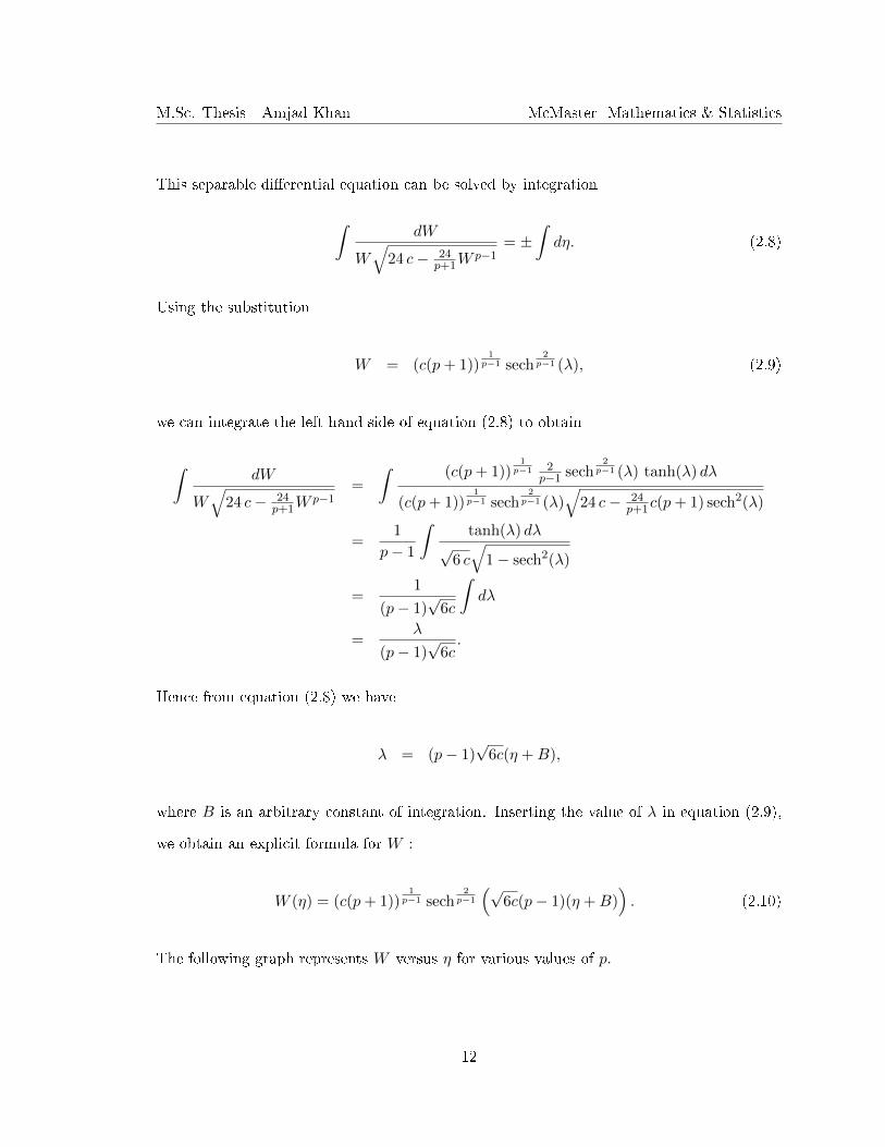
This separable di�erential equation can be solved by integration

∫dW

W√24 c− 24

p+1Wp−1

= ±∫dη. (2.8)

Using the substitution

W = (c(p+ 1))1p−1 sech

2p−1 (λ), (2.9)

we can integrate the left hand side of equation (2.8) to obtain

∫dW

W√24 c− 24

p+1Wp−1

=

∫ (c(p+ 1))1p−1 2

p−1 sech2p−1 (λ) tanh(λ) dλ

(c(p+ 1))1p−1 sech

2p−1 (λ)

√24 c− 24

p+1c(p+ 1) sech2(λ)

=1

p− 1

∫tanh(λ) dλ

√6 c√1− sech2(λ)

=1

(p− 1)√6c

∫dλ

=λ

(p− 1)√6c.

Hence from equation (2.8) we have

λ = (p− 1)√6c(η +B),

where B is an arbitrary constant of integration. Inserting the value of λ in equation (2.9),

we obtain an explicit formula for W :

W (η) = (c(p+ 1))1p−1 sech

2p−1

(√6c(p− 1)(η +B)

). (2.10)

The following graph represents W versus η for various values of p.

12


Figure 2.1: The solitary wave W for p = 2, 3, 4, 5, 6 and B = 0.

2.2 Global well posedness of the gKDV equation

In this section we discuss local and global well posedness for the gKDV equation

Wτ +Wξξξ + (W p)ξ = 0. (2.11)

This equation is called subcritical for p = 2, 3, 4, critical for p = 5 and supercritical for

p ≥ 6, p ∈ N. Local well posedness for the Cauchy problem associated with (2.11) has been

studied by many authors. Below we summarize the local well posedness results.

• It was established in the work of T. Kato [19] that the gKDV equation (2.11) for any

p ≥ 2 is locally well posed in Hs(R) with s > 32 .

• C. Kenig, G. Ponce and L. Vega in [20, 21] showed that the gKDV equation (2.11) is

locally well posed in Hs(R) with s ≥ 34 for p = 2, s ≥ 1

4 for p = 3, s ≥ 112 for p = 4,

and s ≥ p−52(p−1) for p ≥ 5.

The �rst result of global well posedness for the classical KDV equation with p = 2 can

be traced back to the work [22] by J. L. Bona and R. Smith in 1975. Global existence of the

13


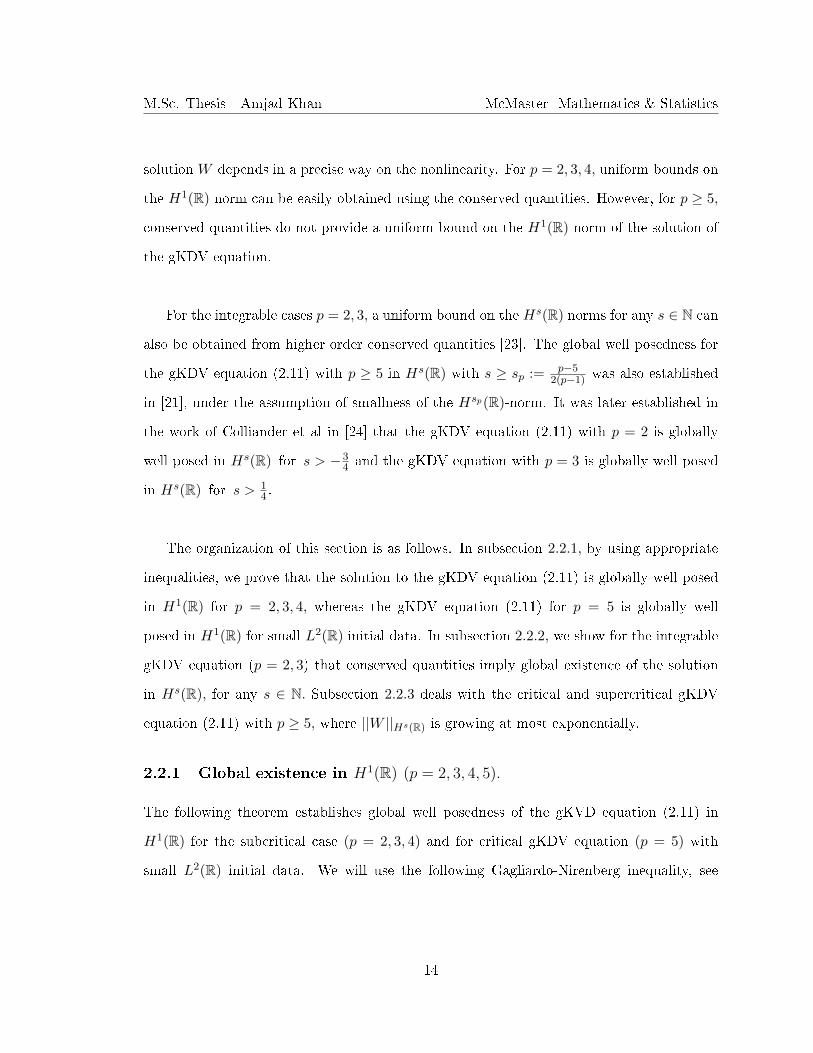
solution W depends in a precise way on the nonlinearity. For p = 2, 3, 4, uniform bounds on

the H1(R) norm can be easily obtained using the conserved quantities. However, for p ≥ 5,

conserved quantities do not provide a uniform bound on the H1(R) norm of the solution of

the gKDV equation.

For the integrable cases p = 2, 3, a uniform bound on the Hs(R) norms for any s ∈ N can

also be obtained from higher order conserved quantities [23]. The global well posedness for

the gKDV equation (2.11) with p ≥ 5 in Hs(R) with s ≥ sp :=p−5

2(p−1) was also established

in [21], under the assumption of smallness of the Hsp(R)-norm. It was later established in

the work of Colliander et al in [24] that the gKDV equation (2.11) with p = 2 is globally

well posed in Hs(R) for s > −34 and the gKDV equation with p = 3 is globally well posed

in Hs(R) for s > 14 .

The organization of this section is as follows. In subsection 2.2.1, by using appropriate

inequalities, we prove that the solution to the gKDV equation (2.11) is globally well posed

in H1(R) for p = 2, 3, 4, whereas the gKDV equation (2.11) for p = 5 is globally well

posed in H1(R) for small L2(R) initial data. In subsection 2.2.2, we show for the integrable

gKDV equation (p = 2, 3) that conserved quantities imply global existence of the solution

in Hs(R), for any s ∈ N. Subsection 2.2.3 deals with the critical and supercritical gKDV

equation (2.11) with p ≥ 5, where ||W ||Hs(R) is growing at most exponentially.

2.2.1 Global existence in H1(R) (p = 2, 3, 4, 5).

The following theorem establishes global well posedness of the gKVD equation (2.11) in

H1(R) for the subcritical case (p = 2, 3, 4) and for critical gKDV equation (p = 5) with

small L2(R) initial data. We will use the following Gagliardo-Nirenberg inequality, see

14


Appendix B.5 in [25]

||W ||p+1Lp+1 ≤ Cgn ||W ||

p+32

L2 ||Wξ||p−12

L2 , (2.12)

where Cgn > 0 is Gagliardo-Nirenberg constant.

Theorem 2.1. The Cauchy problem related to the generalized KDV equation (2.11) is glob-

ally well posed in H1(R), for 2 ≤ p ≤ 4. Furthermore for p = 5 the gKDV equation (2.11)

is well posed in H1(R), with small L2(R) initial data.

Proof. To establish the upper bound on the H1(R) norm, the conservation laws are used.

There are two conserved quantities related to the gKDV equation (2.11), which are given by

Mass: H0 =

∫W 2dξ,

Hamiltonian: H1 =

∫ (W 2ξ −

1

p+ 1W p+1

)dξ, (2.13)

From (2.13), we have

H1 ≥ ||Wξ||2L2 −1

p+ 1||W p+1||L1 . (2.14)

Next, we know that ||W p+1||L1 = ||W ||p+1Lp+1 . By using Gagliardo-Nirenberg inequality (2.12)

we get

H1 ≥ ||Wξ||2L2 −1

p+ 1Cgn||W ||

p+32

L2 ||Wξ||p−12

L2 . (2.15)

15


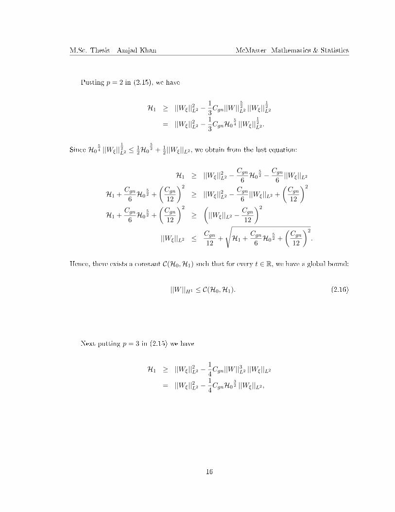
Putting p = 2 in (2.15), we have

H1 ≥ ||Wξ||2L2 −1

3Cgn||W ||

52

L2 ||Wξ||12

L2

= ||Wξ||2L2 −1

3CgnH0

54 ||Wξ||

12

L2 .

Since H054 ||Wξ||

12

L2 ≤ 12H0

52 + 1

2 ||Wξ||L2 , we obtain from the last equation:

H1 ≥ ||Wξ||2L2 −Cgn6H0

52 − Cgn

6||Wξ||L2

H1 +Cgn6H0

52 +

(Cgn12

)2

≥ ||Wξ||2L2 −Cgn6||Wξ||L2 +

(Cgn12

)2

H1 +Cgn6H0

52 +

(Cgn12

)2

≥(||Wξ||L2 −

Cgn12

)2

||Wξ||L2 ≤ Cgn12

+

√H1 +

Cgn6H0

52 +

(Cgn12

)2

.

Hence, there exists a constant C(H0,H1) such that for every t ∈ R, we have a global bound:

||W ||H1 ≤ C(H0,H1). (2.16)

Next putting p = 3 in (2.15) we have

H1 ≥ ||Wξ||2L2 −1

4Cgn||W ||3L2 ||Wξ||L2

= ||Wξ||2L2 −1

4CgnH0

32 ||Wξ||L2 ,

16


so that

H1 +

CgnH 320

8

2

≥ ||Wξ||2L2 − 2Cgn8H0

32 ||Wξ||L2 +

CgnH 320

8

2

H1 +

CgnH 320

8

2

≥

||Wξ||L2 −CgnH

320

8

2

||Wξ||L2 ≤ CgnH320

8+

√√√√√H1 +

CgnH 320

8

2

. (2.17)

Hence, there exists a constant C(H0,H1) such that for every t ∈ R, we have a global bound:

||W ||H1 ≤ C(H0,H1). (2.18)

Similarly for p = 4, equation (2.15) implies

H1 ≥ ||Wξ||2L2 −1

5Cgn||W ||

72

L2 ||Wξ||32

L2

= ||Wξ||2L2 −1

5CgnH0

74 ||Wξ||

32

L2 . (2.19)

Let us denote ||Wξ||12

L2 = x and 15CgnH0

72 = α, then from equation (2.19), we obtain

H1 ≥ x4 − αx3 = f(x). (2.20)

Now f ′(x) = 4x3 − 3αx2 = 0 admits a nonzero root x0 = 3α4 . The function f(x) is

monotonically increasing for x > x0. Hence, for any H0, H1 > 0, there exists a constant

17


C(H0,H1) such that for every t ∈ R, we have a global bound:

||W ||H1 ≤ C(H0,H1). (2.21)

For p = 5, the conserved quantities do not provide a uniform bound in the H1(R) norm.

Inserting p = 5, in equation (2.15), we obtain

H1 ≥ ||Wξ||2L2

(1− 1

6Cgn||W ||4L2

)= ||Wξ||2L2

(1− 1

6CgnH2

0

). (2.22)

Now if the initial L2(R) data is small enough, such that 1 > 16CgnH

20 then

||Wξ||2L2 ≤ H1(1− 1

6CgnH20

) . (2.23)

Hence, for small enough initial data in the L2(R) norm, there exists a constant C(H0,H1)

such that for every t ∈ R, we have a global bound:

||W ||H1 ≤ C(H0,H1). (2.24)

2.2.2 Integrable cases (p = 2, 3)

The generalized KDV equation (2.11) reduces to the integrable KDV equation for p = 2

and to the integrable mKDV equation for p = 3. The integrable KDV equations possess an

in�nite number of conserved quantities [23, 26]. To simplify computations, let us consider

18


the rescaled versions of the KDV (p = 2) and mKDV (p = 3) equations given by

Wτ +Wξξξ +WWξ = 0, (2.25)

and

Wτ +Wξξξ +W 2Wξ = 0, (2.26)

respectively. The following result establishes the global existence of gKDV equation for

p = 2, 3 in Hs(R) for every s ∈ N, such that the Hs(R) norm of the global solution is

bounded from above for all times.

Theorem 2.2. There exists a unique global solution to the KDV equation (2.25) and mKDV

equation (2.26) in Hs(R) for every s ∈ N. In particular, there exists a constant Cs such that

for every t ∈ R,

||W ||Hs(R) ≤ Cs.

Proof. It is well known, see [26], that the KDV equation (2.25) possess the following con-

served quantities in addition to the mass and Hamiltonian in (2.13):

H2 =

∫ (W 2ξξ −

5

3WW 2

ξ +5

36W 4

)dξ,

H3 =

∫ (W 2ξξξ −

7

3WW 2

ξξ +35

18W 2W 2

ξ −7

108W 5

)dξ,

H4 =

∫ (W 2ξξξξ +

15

17W 3ξξ − 3WW 2

ξξξ −35

36W 4ξ +

7

2W 2W 2

ξξ −35

18W 3W 2

ξ +7

216W 6

)dξ.

By using Sobolev inequality, we obtain for H2 :

H2 = ||Wξξ||2L2 −5

3

∫WW 2

ξ dξ +5

36||W ||4L4 ,

≥ ||Wξξ||2L2 −5

3C||W ||3H1 ,

19


so that

||Wξξ||2L2 ≤ H2 +5

3C||W ||3H1 .

Since ||W ||H1 is controlled by (2.16), there exists a constant C(H0,H1,H2) such that for

any t ∈ R, we have a global bound:

||W ||H2 ≤ C(H0,H1,H2). (2.27)

Similarly, we obtain for H3 with Sobolev inequality

H3 = ||Wξξξ||2L2 −7

3

∫WW 2

ξξdξ +35

18

∫W 2W 2

ξ dξ −7

108

∫W 5dξ

≥ ||Wξξξ||2L2 −7

3C1||W ||3H2 −

7

108C2||W ||5H1 ,

so that

||Wξξξ||2L2 ≤ H3 +7

3C1||W ||3H2 +

7

108C2||W ||5H1 .

Since ||W ||H2 is now controlled by (2.27), there exists a constant C(H0,H1,H2,H3) such

that for every t ∈ R, we have a global bound:

||W ||H3 ≤ C(H0,H1,H2,H3),

The method applies to H4, etc, to yield a global solution in H4(R), etc.

20


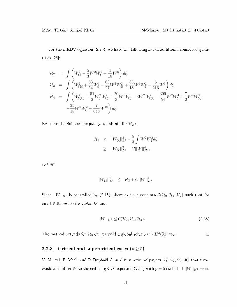
For the mKDV equation (2.26), we have the following list of additional conserved quan-

tities [26]:

H2 =

∫ (W 2ξξ −

5

3W 2W 2

ξ +1

18W 6

)dξ.

H3 =

∫ (W 2ξξξ +

63

54W 4ξ −

63

27W 2W 2

ξξ +35

18W 4W 2

ξ −5

216W 6

)dξ.

H4 =

∫ (W 2ξξξξ +

51

3W 2ξW

2ξξ +

20

3W W 3

ξξ − 3W 2W 2ξξξ −

399

54W 2W 4

ξ +7

2W 4W 2

ξξ

−35

18W 6W 2

ξ +7

648W 10

)dξ.

By using the Sobolev inequality, we obtain for H2 :

H2 ≥ ||Wξξ||2L2 −5

3

∫W 2W 2

ξ dξ

≥ ||Wξξ||2L2 − C||W ||4H1 ,

so that

||Wξξ||2L2 ≤ H2 + C||W ||4H1 .

Since ||W ||H1 is controlled by (2.18), there exists a constant C(H0,H1,H2) such that for

any t ∈ R, we have a global bound:

||W ||H2 ≤ C(H0,H1,H2). (2.28)

The method extends for H3 etc, to yield a global solution in H3(R), etc.

2.2.3 Critical and supercritical cases (p ≥ 5)

V. Martel, F. Merle and P. Raphael showed in a series of papers [27, 28, 29, 30] that there

exists a solution W to the critical gKDV equation (2.11) with p = 5 such that ||W ||H1 →∞

21


as τ ↑ T, where T < +∞. This indicates a possibility of a blow up in a �nite time . On the

other hand, Theorem 2.1 excludes blow up for p = 5 if the initial data is small in the L2(R)

norm. Further, numerical simulations by D. B. Dix and W. R. McKinney [31] suggest blow

up in a �nite time for the supercritical gKDV equation (2.11) with p ≥ 6.

The following result of C. Kenig, G. Ponce, and L. Vega [21] eliminates blow up in a

�nite time for small-norm initial data. First we introduce the following notations. Let

1 ≤ p, q ≤ ∞ and f : R× [−τ, τ ]→ R. De�ne

||f ||LpξLqτ ≡

(∫ ∞−∞

(∫ τ

−τ|f(ξ, τ)|qdτ

) pq

dξ

) 1p

and

||f ||LqτLpξ ≡

(∫ τ

−τ

(∫ ∞−∞|f(ξ, τ)|pdξ

) qp

dτ

) 1q

.

Theorem 2.3. Let p = 5. There exists δ > 0 such that for any initial W0 ∈ L2(R) with

||W0||L2 < δ,

there exists a unique strong solution W of the Cauchy problem related to the gKDV equation

(2.11) satisfying

W ∈ C(R;L2(R)) ∩ L∞(R;L2(R)),

and

∣∣∣∣∣∣∣∣∂W∂ξ∣∣∣∣∣∣∣∣L∞ξ L

2τ

≤ D <∞. (2.29)

Similar results also remain true for p ≥ 6, see [21]. Our next result shows that the upper

bound on the solution W in the Hs(R) norm depends on τ and grows as t → ∞. It is

22


important for justi�cation analysis to understand the growth rate of ||W ||Hs(R). First, we

note the following Gronwall's inequality, see Appendix B.6 in [25].

Lemma 2.1. Let C ≥ 0, k(t) be a given continuous non-negative function for all t ≥ 0,

and y(t) be a continuous function satisfying the integral inequality

0 ≤ y(t) ≤ C +

∫ t

0k(t′)y(t′)dt′.

Then

y(t) ≤ C e∫ t0 k(t

′)dt′ for all t ≥ 0. (2.30)

Theorem 2.4. For p = 5. Under the assumption of Theorem 2.3, the upper bound for the

Hs(R) norm of the solution W of the gKDV equation (2.11), depends on τ and grows at

most exponentially as τ →∞, that is, there exists a constant cs > 0 and ks > 0 such that

||W ||Hs(R) ≤ cseks∫ τ0 ||Wξ||L∞dτ ′ . (2.31)

Proof. For p = 5, we di�erentiate the gKDV equation (2.11) twice with respect to ξ,multiply

by Wξξ and then integrate with respect to ξ, to obtain

∫WτξξWξξdξ +

∫Wξ5Wξξdξ + 60

∫W 2W 3

ξWξξdξ + 60

∫W 3WξW

2ξξdξ

+5

∫W 4WξξξWξξdξ = 0. (2.32)

Using integration by parts and zero boundary conditions, it can be shown that the term∫Wξ5Wξξdξ = 0. Similarly, using integration by parts and zero boundary conditions, the

term 5∫W 4WξξξWξξdξ = −10

∫W 3WξW

2ξξdξ. Hence from (2.32), we have

1

2

d

dτ

∫W 2ξξdξ − 30

∫WW 5

ξ dξ + 50

∫W 3WξW

2ξξdξ = 0. (2.33)

23


Let Q2 = ||Wξξ||L2 . Using Holder inequality, we rewrite (2.33) as follows:

Q2dQ2

dτ≤ 30||W ||L∞ ||Wξ||L∞ ||Wξ||4L4 + 50||W ||3L∞ ||Wξ||L∞ Q2

2.

By Gagliardo-Nirenberg inequality (2.12), we have

||W ||4L4 ≤ Cgn||Wξ||3L2 ||Wξξ||2L2 ,

so that

dQ2

dτ≤ 30Cgn||W ||L∞ ||Wξ||3L2 ||Wξ||L∞ + 50||W ||3L∞ ||Wξ||L∞ Q2 (2.34)

Thanks to Theorem 2.1, there exists a constant k1, k2 > 0 such that

30Cgn||W ||L∞ ||Wξ||3L2 ≤ k1, 50||W ||3L∞ ≤ k2.

Therefore, we have

d

dτ

(e−k2

∫ τ0 ||Wξ||L∞dτ ′Q2(τ)

)≤ k1||Wξ||L∞e−k2

∫ τ0 ||Wξ||L∞dτ ′ . (2.35)

Now using Gronwall's inequality (2.30), we get

Q2(τ) ≤(k1k2

+Q2(0)

)ek2

∫ τ0 ||Wξ||L∞dτ ′

which yields the bound (2.31) for s = 2 and large τ.

Next we show that ||W ||H3(R) is also growing at the same rate. Again we di�erentiate

the gKDV equation (2.11) three times with respect to ξ, multiply byWξξξ and then integrate

24


with respect to ξ, to obtain

∫WτξξξWξξξdξ +

∫Wξ6Wξξξdξ + 120

∫WW 4

ξWξξξdξ + 360

∫W 2W 2

ξWξξWξξξdξ

+ 60

∫W 3W 2

ξξWξξξ + 80

∫W 3WξW

2ξξξdξ + 5

∫W 4Wξ4Wξξξdξ = 0. (2.36)

Using integration by parts and zero boundary condition, for W and all of its derivatives,

it can be shown that the term∫Wξ6Wξξξdξ = 0. Similarly, using integration by parts and

zero boundary conditions, we arrive at

60

∫W 3W 2

ξξWξξξdξ = −15∫WW 4

ξWξξξdξ + 60

∫W 2W 2

ξWξξWξξξdξ

5

∫W 4Wξ4Wξξξdξ = −10

∫W 3WξW

2ξξξdξ.

From (2.36), we have

1

2

d

dτ

∫W 2ξξξdξ ≤ 105

∫WW 4

ξWξξξdξ + 420

∫W 2W 2

ξWξξWξξξdξ

+ 70

∫W 3WξW

2ξξξdξ.

Hence

1

2

d

dτ||Wξξξ||2L2 ≤ 105||WW 3

ξ ||L∞ ||Wξ||L2 ||Wξξξ||L2 + 420||W 2W 2ξ ||L∞ ||Wξξ||L2 ||Wξξξ||L2

+ 70||W 3Wξ||L∞ ||Wξξξ||2L2 . (2.37)

Let Q3 = ||Wξξξ||L2 . Then, the di�erential inequality (2.37) can be written as

Q3dQ3

dτ≤ 105||WW 3

ξ ||L∞ ||Wξ||L2Q3 + 420||W 2W 2ξ ||L∞Q2Q3

+ 70||W 3Wξ||L∞Q23,

25


so that

dQ3

dτ≤ 105||WW 3

ξ ||L∞ ||Wξ||L2 + 420||W 2W 2ξ ||L∞Q2 + 70||W 3Wξ||L∞Q3

≤ Const1 + Const2||Wξ||L∞ Q22 + Const3||Wξ||L∞Q3, (2.38)

thanks to Sobolev's inequality and previous bounds. Using a similar technique as explained

above, we obtain (2.31) for s = 3. The same method applies to ||W ||H4(R), etc.

26

Chapter 3

Approximations of the

Fermi-Pasta-Ulam lattice dynamics

In this chapter, the relation between the FPU lattice equation (1.4) and the gKDV equation

(1.11) is established. The FPU equation (1.4) can be written as the FPU system,

un = qn+1 − qn,

qn = un − un−1 + ε2(upn − upn−1

),n ∈ Z. (3.1)

Any solution (u, q) ∈ C1(R, l2(Z)) of the FPU system (3.1) provides a C2(R, l2(Z)) solution

u to the FPU equation (1.4). The FPU lattice system (3.1) admits the conserved energy

H :=1

2

∑n∈Z

(q2n + u2n +

2ε2

p+ 1up+1n

). (3.2)

In the next result, we prove local (in time) well-posedness of the Cauchy problem associated

with the FPU system (3.1) in the sequence space l2(Z). In what follows, the sequences

{un(t)}n∈Z, {qn(t)}n∈Z in the space l2(Z) are denoted by u(t) and q(t) respectively. To

prove the local existence result, we recall the statement of the Banach �xed point theorem.

27


De�nition 3.1. Let M be a closed non-empty set in Banach space X. The operator A :

M →M is called a contraction if there is 0 ≤ q < 1 such that

∀x, y ∈M : ||Ax−Ay||X ≤ q||x− y||X .

Theorem 3.1. (Banach �xed point theorem) Let M be a closed non-empty set in a

Banach space X and let A :M →M be a contraction operator. Then, there exists a unique

�xed point of A in M , that is, there exists a unique x ∈M such that A(x) = x.

By using Banach �xed point theorem, we establish local well-posedness of the Cauchy

problem for the FPU system (3.1).

Theorem 3.2. There exists a local solution (u(t), q(t)) ∈ C1([−t0, t0], l2(Z)

)for some

t0 > 0, to the Cauchy problem associated with the FPU system (3.1) for initial data (u0, q0) ∈

l2(Z) such that u(0) = u0 and q(0) = q0.

Proof. To prove the local well-posedness of the FPU system (3.1), we write the system in

the integral form as

u(t) = u(0) +∫ t0 ∇+ q(s)ds,

q(t) = q(0) +∫ t0 ∇− u(s)ds+ ε2

∫ t0 ∇− u

p(s)ds,t ∈ [−t0, t0], (3.3)

where (∇+ q)n = qn+1 − qn and (∇− u)n = un − un−1. The space X = L∞([−t0, t0], l2(Z))

is a Banach space. We consider an open ball Bδ(0) ⊂ X, with radius δ > 0 and centered at

0. It is obvious that ||∇± q||l2 ≤ 2||q||l2 .

First we show that the right hand side of the integral equation (3.3) de�nes a Lipschitz

28


continuous map in the ball Bδ(0) with δ > 0. Indeed, we have

||u(0) +∫ t

0∇+q(s)ds||X = sup

t∈[−t0,t0]

∣∣∣∣∣∣∣∣u(0) + ∫ t

0∇+ q(s)ds

∣∣∣∣∣∣∣∣l2

≤ ||u(0)||l2 + supt∈[−t0,t0]

∣∣∣∣∣∣∣∣∫ t

0∇+ q(s)ds

∣∣∣∣∣∣∣∣l2

≤ ||u(0)||l2 + 2

∫ t0

0||q(s)||l2 ds

≤ ||u(0)||l2 + 2t0 ||q(t)||X , (3.4)

and

|| q(0) +∫ t

0∇− u(s)ds+ ε2

∫ t

0∇−up(s)ds

∣∣∣∣∣∣∣∣X

≤ ||q(0)||l2 + supt∈[−t0,t0]

∣∣∣∣∣∣∣∣∫ t

0∇−u(s)ds

∣∣∣∣∣∣∣∣l2+ ε2 sup

t∈[−t0,t0]

∣∣∣∣∣∣∣∣∫ t

0∇− up(s)ds

∣∣∣∣∣∣∣∣l2

≤ ||q(0)||l2 + 2

∫ t0

0||u(s)||l2 ds+ 2ε2

∫ t0

0||up(s)||l2 ds

≤ ||q(0)||l2 + 2t0||u(t)||X + 2ε2t0||u(t)||pX . (3.5)

In the last inequality we used the Banach algebra property of X = L∞([−t0, t0], l∞(Z)).

From the bounds (3.4) and (3.5) we conclude that for every δ > 0 there is a su�ciently

small t0 > 0 such that the operator A maps Bδ(0) to itself, where A represents the right

hand side of the integral equation (3.3).

Next we show that by choosing su�ciently small t0 > 0, the Lipzchitz constant corre-

sponding to the map A : Bδ(0) → Bδ(0) can be made smaller then unity, which results in

29


a contraction of A in Bδ(0). We obtain

∣∣∣∣Au′ −Au′′∣∣∣∣X

= supt∈[−t0,t0]

∣∣∣∣∣∣∣∣∫ t

0∇+ q

′(s)ds−∫ t

0∇+q

′′(s)ds

∣∣∣∣∣∣∣∣l2

= supt∈[−t0,t0]

∣∣∣∣∣∣∣∣∫ t

0∇+

(q′ − q′′

)(s)ds

∣∣∣∣∣∣∣∣l2

≤ 2

∫ t0

0

∣∣∣∣(q′ − q′′) (s)∣∣∣∣l2ds

≤ 2t0∣∣∣∣q′ − q′′∣∣∣∣

X

= k1∣∣∣∣q′ − q′′∣∣∣∣

X, (3.6)

where k1 = 2t0, so that if t0 <12 then k1 < 1. Also we have

∣∣∣∣Aq′ −Aq′′∣∣∣∣X

= supt∈[−t0,t0]

∣∣∣∣∣∣∣∣∫ t

0∇−

(u′ − u′′

)(s)ds+ ε2

∫ t

0∇−(u′p − u′′p)(s)ds

∣∣∣∣∣∣∣∣l2

≤ 2

∫ t0

0

∣∣∣∣(u′ − u′′) (s)∣∣∣∣l2ds+ 2ε2

∫ t0

0

∣∣∣∣(u′p − u′′p)(s)∣∣∣∣l2ds

≤ 2t0∣∣∣∣(u′ − u′′) (s)∣∣∣∣

X+ 2ε2t0

∣∣∣∣(u′p − u′′p)(s)∣∣∣∣X

≤ 2t0(1 + ε2

∣∣∣∣(u′p−1 + ...+ u′′p−1)∣∣∣∣X

) ∣∣∣∣u′ − u′′∣∣∣∣X

≤ k2∣∣∣∣u′ − u′′∣∣∣∣

X, (3.7)

where k2 = 2t0(1 + ε2pδp−1

), so that if t0 <

12(1+ε2pδp−1)

then k2 < 1. From (3.6) and (3.7)

we conclude that if

t0 ≤ min

(1

2,

1

2 (1 + ε2pδp−1)

)then k = max(k1, k2) < 1, showing that A : Bδ(0)→ Bδ(0) is a contraction. By the Banach

�xed point theorem, there exists a unique �xed point (u,q) in Bδ(0) such that

A(u,q) = (u,q).

Since ∇± are bounded operators, the integral of a continuous function gives a continuously

30


di�erentiable function. Hence, (u(t),q(t)) ∈ C1([−t0, t0], l2(Z)).

Remark 3.1. If p is an odd integer, then the local solution (u(t), q(t)) ∈ C([−t0, t0], l2(Z)

)can be continued globally in time by using the energy conservation (3.2).

3.1 Derivation of the gKDV equation and residual terms

We shall recover the derivation of the gKDV equation (1.11). In our present treatment, we

work with the FPU lattice system (3.1). Let us consider the decomposition

un(t) =W (ε(n− t), ε3t) + Un(t), qn = Pε(ε(n− t), ε3t) + Pn(t), n ∈ Z, (3.8)

where W (ξ, τ) is a smooth solution to the gKDV equation (1.11). Therefore, W is indepen-

dent of ε. On the other hand, Pε(ξ, τ) depends on ε. This function can be found from the

�rst equation of system (3.1), which is rewritten as

Pε(ξ + ε, τ)− Pε(ξ, τ) = −ε∂ξW (ξ, τ) + ε3∂τW (ξ, τ). (3.9)

We look for an approximate solution Pε to this equation, under the form

Pε := P 0 + εP 1 + ε2P 2 + ε3P 3, (3.10)

with functions P j decaying to zero as ξ →∞. Inserting (3.10) into (3.9), we get

ε∂ξPε(ξ, τ) +ε2

2!∂ξξPε(ξ, τ) +

ε3

3!∂ξξξPε(ξ, τ) +

ε4

4!∂ξξξξPε(ξ, τ) + ...

= −ε∂ξW (ξ, τ) + ε3∂τW (ξ, τ). (3.11)

31


Collecting the terms in powers of ε, we get

O(ε) : ∂ξP0 = −∂ξW

O(ε2) : ∂ξP1 +

1

2∂ξξP

0 = 0

O(ε3) : ∂ξP2 +

1

2∂ξξP

1 +1

6∂ξξξP

0 =−124∂ξξξW −

1

2∂ξW

p

O(ε4) : ∂ξP3 +

1

2∂ξξP

2 +1

6∂ξξξP

1 +1

24∂ξξξξP

0 = 0.

These equations are satis�ed when

P 0 = −W

P 1 =1

2∂ξW

P 2 =−18∂ξξW −

1

2W p

P 3 =1

48∂ξξξW +

1

4∂ξW

p.

When a solution W to the gKDV equation (1.11) is given, we can de�ne

Pε = −W +ε

2Wξ −

ε2

8Wξξ −

ε2

2W p +

ε3

48Wξξξ +

ε3

4pW p−1Wξ. (3.12)

By construction, the pair of functions (W,Pε) solves the �rst equation in system (3.1) up

to the O(ε4) terms. Substituting the decomposition (3.8) into the FPU lattice system (3.1),

we obtain the evolutionary problem for the error terms

Un = Pn+1 − Pn +Res1n,

Pn = Un − Un−1 + pε2(W (ε(n− t), ε3t))p−1Un −W (ε(n− 1− t), ε3t)p−1Un−1

)+Rn(W,U)(t) +Res2n(t),

(3.13)

32


where

Rn(W,U)(t) := ε2[{W (ε(n− t), ε3t) + Un(t)}p −W (ε(n− t), ε3t)p − pW (ε(n− t), ε3t)p−1Un

]− ε2[{W (ε(n− 1− t), ε3t) + Un−1(t)}p −W (ε(n− 1− t), ε3t)p

− pW (ε(n− 1− t), ε3t)p−1Un−1],

and

Res1n = Pε(ε(n+ 1− t), ε3t)− Pε(ε(n− t), ε3t) + ε∂ξW (ε(n− t), ε3t)− ε3∂τW (ε(n− t), ε3t),

Res2n = ε∂ξPε(ε(n− t), ε3t)− ε3∂τPε(ε(n− t), ε3t) +W (ε(n− t), ε3t)−W (ε(n− 1− t), ε3t)

+ε2[W (ε(n− t), ε3t)p −W (ε(n− 1− t), ε3t)p].

3.2 Bounds on residual terms

In this section we will develop bounds on the residual terms. To establish these bounds we

recall the following result, proved in Lemma 5.1 in [18].

Lemma 3.1. There exists C > 0 such that for all X ∈ H1 and ε ∈ (0, 1],

||x||l2 ≤ Cε−12 ||X||H1 (3.14)

where xn := X(εn), n ∈ Z.

We also use the following result from Chapter 4 [32],

Lemma 3.2. Suppose f : [a, b]→ R is of class Cn, and f (n+1) is integrable. Then ∀x ∈ [a, b]

we have f(x) = Pn(x) +Rn(x) where

Pn(x) =

n∑k=0

f (k)(a)(x− a)k

k!(3.15)

33


and

Rn(x) =(x− a)n+1

n!

∫ 1

0(1− r)nf (n+1)(a+ r(x− a))dr. (3.16)

The next result provide bounds on R, Res1 and Res2 in the time evolutionary system

(3.13).

Lemma 3.3. Let W ∈ C([−τ0, τ0], H6(R)

)be a solution to the gKDV equation (1.11)

for some τ0 > 0. Then, there exist positive constants CW and CW,U , such that for all t ∈

[−τ0ε−3, τ0ε−3] and ε ∈ (0, 1],

∣∣∣∣Res1∣∣∣∣l2+∣∣∣∣Res2∣∣∣∣

l2≤ CW ε

92 , (3.17)

and

||R(W,U)||l2 ≤ ε2CW,U ||U||2l2 , (3.18)

where CW and CW,U are constant proportional to ||W ||H6 + ||W ||pH6 and ||W ||p−2

H6 + ||U||p−2l2

respectively.

Proof. To prove the bound (3.17), we use (3.12) in

Res1n = Pε(ε(n+ 1− t), ε3t)− Pε(ε(n− t), ε3t) + ε∂ξW (ε(n− t), ε3t)− ε3∂τW (ε(n− t), ε3t).

By expanding the resulting expression with Taylor's theorem, we obtain

Res1n = ε5(

1

480Wξ5(ξ, τ) +

1

24p(p− 1)(p− 2)W (ξ, τ)p−3Wξ(ξ, τ)

3

+1

8p(p− 1)W (ξ, τ)p−2Wξ(ξ, τ)Wξξ(ξ, τ) +

1

24pW (ξ, τ)p−1Wξξξ(ξ, τ)

)+O(ε6),

34


which can be written in the closed form (3.16) as follows:

Res1n =1

480ε5∫ 1

0(1− r)4∂ξξξξξW

(ε(n− t+ r), ε3t

)dr

+1

24ε5∫ 1

0(1− r)2∂ξξξW p

(ε(n− t+ r), ε3t

)dr.

Now using the bound (3.14) we get

∣∣∣∣Res1∣∣∣∣l2≤ 1

480ε5∫ 1

0(1− r)4||∂ξξξξξW ||l2dr +

1

24ε5∫ 1

0(1− r)2||∂ξξξW p||l2dr

≤ C

2400ε92 ||∂ξξξξξW ||H1 +

C

72ε92 ||∂ξξξW p||H1

≤ C1ε92(||W ||H6 + ||W ||pH6

).

Next, we expand the expression

Res2n = ε∂ξPε(ε(n− t), ε3t)− ε3∂τPε(ε(n− t), ε3t) +W (ε(n− t), ε3t)−W (ε(n− 1− t), ε3t)

+ε2(W (ε(n− t), ε3t)p −W (ε(n− 1− t), ε3t)p),

in Taylor's series. The coe�cients of ε0, ε1, ε2 vanish, whereas the coe�cient of ε3 also

vanishes by using the fact thatW is a solution to the gKDV equation (1.11). The coe�cient

of ε4 also vanishes in the following computation:

1

48Wξξξξ +

1

4p(p− 1)W p−2Wξξ +

1

4pW p−1W 2

ξ −1

2pW p−1Wξξ −

1

2p(p− 1)W p−2W 2

ξ −1

2Wξτ

=−148Wξξξξ −

1

4p(p− 1)W p−2Wξξ −

1

4pW p−1W 2

ξ −1

2Wξτ

=−14∂ξ

(2Wτ +

1

12Wξξξ + pW p−1Wξ

)= 0.

35


Finally, the coe�cient of O(ε5) is given by

1

5!Wξ5(ξ, τ) +

p

3!W (ξ, τ)p−1Wξξξ(ξ, τ) +

p(p− 1)

2Wξ(ξ, τ)Wξξ(ξ, τ)W (ξ, τ)p−2

+p(p− 1)(p− 2)

3!W (ξ, τ)p−3Wξ(ξ, τ)

3 +1

8∂τ (Wξξ(ξ, τ)) +

1

2∂τ (W (ξ, τ)p) .

Now using the bound (3.14), and following the same lines as for Res1n, we get

∣∣∣∣Res2∣∣∣∣l2≤ C2ε

92(||W ||H6 + ||W ||pH6

).

IfW ∈ C([−τ0, τ0], H6(R)), then there exists a positive constant CW = C3

(||W ||H6 + ||W ||pH6

),

with C3 = max(C1, C2), such that the bound (3.17) holds.

Next, we prove the bound (3.18). To do so, we write Rn(W,U)(t) in the form

Rn(W,U)(t) = ε2

(p∑

k=2

(p

k

)W (ε(n− t), ε3t)p−kUn(t)k

)

−ε2(

p∑k=2

(p

k

)W (ε(n− 1− t), ε3t)p−kUn−1(t)k

). (3.19)

Interpolating between the end point terms, we obtain for some C > 0:

||R(W,U)(t)||l2 ≤ C ε2(||W (ε(n− t), ε3t)p−2U2

n(t)||2l2 + ||Up||l2

)≤ C ε2||W (ε(.− t), ε3t)||p−2L∞ ||U(t)||

2l2 + C ε2||U||p−2l∞ ||U||

2l2

≤ C ε2(||W ||p−2

H6 + ||U||p−2l2

)||U||2l2 ,

which proves the bound (3.18) with CW,U = C(||W ||p−2

H6 + ||U||p−2l2

).

36


3.3 Justi�cation of gKDV equation on the standard time scale

We now formulate the main justi�cation result. It is proved by using the estimates developed

in Section 3.2 and the energy method.

Theorem 3.3. Let W ∈ C([−τ0, τ0], H6(R)) be a solution to the gKDV equation (1.11) for

any τ0 > 0. Then there exists positive constants ε0 and C0 such that, for all ε ∈ (0, ε0), when

initial data (uin,ε, qin,ε) ∈ l2(Z) are given such that

||uin,ε −W (ε·, 0)||l2 + ||qin,ε − Pε(ε·, 0)||l2 ≤ ε32 , (3.20)

the unique solution (uε, qε) to the FPU lattice equation (3.1) with initial data (uin,ε, qin,ε)

belongs to C1([−τ0ε−3, τ0ε−3], l2(Z)) and satisfy for every t ∈ [−τ0ε−3, τ0ε−3] :

||uε(t)−W (ε(· − t), ε3t)||l2 + ||qε(t)− Pε(ε(· − t), ε3t)||l2 ≤ C0ε32 . (3.21)

Proof. For ε0 small enough and for the initial data (uin, qin) satisfying the bound (3.20), we

can de�ne a local in time solution (u, q) to the FPU lattice system (3.1), which is decomposed

according to (3.8). Let us de�ne for a �xed C > 0 :

TC := sup{T ∈ [0, τ0ε

−3] : Q(t) ≤ C ε, t ∈ [−T, T ]}, (3.22)

where Q = E12 and E is the energy like quantity given by

E(t) :=1

2

∑n∈Z

[P2n + U2

n + ε2pW (ε(n− t), ε3t)p−1U2n(t)

]. (3.23)

We prove that for �xed C > 0 and ε0 small enough, we have TC = τ0ε−3. From (3.23), we

37


can write

2E(t) =

(||P(t)||2l2 + ||U(t)||

2l2 + ε2

∑n∈Z

pW (ε(n− t), ε3t)p−1Un(t)2)

≥ ||P(t)||2l2 + ||U(t)||2l2(1− ε2||pW (ε(· − t), ε3t)p−1||L∞

),

hence for ε0 < min

(1, ||2pW (ε(· − t))p−1||−

12

L∞

), and ε ∈ (0, ε0), we have

||P||2l2 + ||U||2l2 ≤ 4E(t), t ∈ (0, TC). (3.24)

Taking the derivative of E with respect to t, we obtain

dE

dt=∑n∈Z

[PnRn(W,U) + PnRes2n(t) + Un(t)Res1n(t) + ε2pW p−1(ε(n− t), ε3t)Un(t)Res1n(t)

+ ε2

2 p(p− 1)W p−2(ε(n− t), ε3t)(−ε∂ξ + ε3∂τ )W (ε(n− t), ε3t)U2n(t)].

Then using Cauchy-Schwartz inequality, we estimate

∣∣∣∣dEdt∣∣∣∣ ≤ ||P||l2 ||R(W,U)||l2 + ||P||l2 ||Res2(t)||l2 + 3

2||U(t)||l2 ||Res1(t)||l2 + ε3CW ||U(t)||2l2 ,

where CW = C||W ||p−2H6

(||W ||H6 + ||W ||p

H6

). Using Lemma 3.2 and inequality (3.24), we

can write

∣∣∣∣dEdt∣∣∣∣ ≤ 8CW,Uε

2E32 + 5CW ε

92E

12 + 4CW ε

3E, (3.25)

≤ 2 CW,UE12

(ε92 + ε3E

12 + ε2E

).

where CW,U = max(4CW,U ,

52CW , 2CW

). Choosing Q = E

12 , the energy balance equation

38


can be written in the form

∣∣∣∣dQdt∣∣∣∣ ≤ CW,U

(ε92 + ε3Q+ ε2Q2

),

≤ CW,U

(ε92 + (1 + C)ε3Q

).

The latter inequality remains true as long as TC is de�ned by (3.22) so that ||U||l2 ≤ Cε,

for some C > 0. Next, Q(t) can be written for t > 0 as

Q(t) = Q(0) +∫ t

0Q′(s)ds,

≤ Q(0) + CW,U

∫ t

0

(ε92 + (1 + C)ε3Q(s)

)ds,

= Q(0) + CW,Uε92 t+ CW,U (1 + C)

∫ t

0ε3Q(s)ds.

By using Gronwall's inequality (2.30), we obtain

Q(t) ≤(Q(0) + CW,Uε

92 |t|)e(1+C)ε3CW,U |t|.

The initial bound (3.20) ensures that Q(0) ≤ C0ε32 . Hence

Q(t) ≤(C0 + CW,Uτ0

)ε32 e(1+C)CW,Uτ0 , t ∈ (−TC , TC). (3.26)

Finally, choosing ε0 su�ciently small such that the bound ||U(t)||l2 ≤ C ε is preserved, which

is always possible because ε32 << ε, we obtain a continuation of the local solution to the

time scale TC = τ0ε−3.

3.4 Justi�cation of gKDV equation on the extended time scale

In this section, we extend the justi�cation analysis to a longer time interval for solution of

the gKDV equation (1.11). We consider two cases here: the integrable case with p = 2, 3 and

39


the critical and supercritical case with p ≥ 5. In the �rst case, we show that the time interval

of the solution of the gKDV equation (1.11) can be extended by a logarithmic factor. In the

second case, we show that the time interval can only be extended by a double logarithmic

factor. In both the cases, the time τ0 used in Section 3.3 becomes ε-dependent.

Case 1: Integrable gKDV (p = 2, 3)

Recall from Chapter 2 (Theorem 2.2) that the upper bound on the H6(R) norm of the

solution to the gKDV equation (1.11) with p = 2, 3 can be bounded by a time-independent

constant. Therefore,

δ = supτ∈[−τ0,τ0]

||W (t)||H6 (3.27)

is independent of τ0. The following theorem speci�es the extension of the time scale by a

logarithmic factor, where the gKDV equation (1.11) with p = 2, 3 can be justi�ed.

Theorem 3.4. Let W ∈ C(R, H6(R)) be a global solution to the gKDV equation (1.11) with

p = 2, 3. For �xed r ∈(0, 1

2

), there exists positive constants ε0 and C0 such that, for all

ε ∈ (0, ε0), when initial data (uin,ε, qin,ε) ∈ l2(Z) are given such that


the unique solution (uε, qε) to the FPU lattice equation (3.1) with initial data (uin,ε, qin,ε)

belongs to C1([− r| log(ε)|

k0ε−3, r| log(ε)|k0

ε−3], l2(Z)

), where an ε-independent ko is de�ned by

(3.33) below and (uε, qε) satisfy

||uε(t)−W (ε(· − t), ε3t)||l2 + ||qε(t)− Pε(ε(· − t), ε3t)||l2 ≤ C0ε32−r, (3.29)

for every t ∈[− r| log(ε)|

k0ε−3, r| log(ε)|k0

ε−3].

40


Proof. By Theorem 3.2, for ε0 small enough and for the initial data (uin,ε, qin,ε) satisfying

the bound (3.28), we can de�ne local in time solution of the FPU system (3.1), which is

decomposed according to equation (3.8). Let us de�ne for C > 0 and r ∈(0, 1

2

)TC,r := sup

{T ∈ [0, τ0(ε)ε

−3] : Q(t) ≤ Cε32−r, t ∈ [−T, T ]

}, (3.30)

where τ0(ε) is de�ned by (3.36) below. By de�ning an energy like quantity (3.23) and

following the same agrement as in the proof of Theorem 3.3, see the estimate (3.25), we

arrive at the following equation

∣∣∣∣dQdt∣∣∣∣ = CW,Uε

2Q2 + CW ε3Q+ CW ε

92 , (3.31)

whereQ = E12 . From Lemma 3.2, we know that the constants CW and CW,U are proportional

to ||W ||H6 + ||W ||pH6 and ||W ||p−2

H6 + ||U||p−2l2

, respectively. It was also established in the

proof of Theorem 3.3 that the constant CW is proportional to ||W ||p−1H6 + ||W ||2p−2

H6 . Using

equation (3.27) and the estimate ||U||l2 ≤ 2Q in equation (3.31), we obtain

∣∣∣∣dQdt∣∣∣∣ ≤ C1

(δp−1 + δ2p−2 +

1

ε(δp−2 +Qp−2)Q

)ε3Q+ C2 (δ + δp) ε

92 , (3.32)

where C1 and C2 are positive constants. Since δ is independent of τ, there exists an ε-

independent k0 > 0 such that

C1

(δp−1 + δp−2 +

1

ε(δp−2 +Qp−2)Q

)≤ k0, (3.33)

as long as t ∈ [−TC,r(ε), TC,r(ε)]. Using inequality (3.33) in the inequality (3.32), we obtain

∣∣∣∣dQdt∣∣∣∣ ≤ ε3k0Q+ Cδε

92 , (3.34)

41


where Cδ depends on δ. From (3.34), we obtain

d

dt

(e−ε

3k0tQ(t))≤ Cδε

92 e−ε

3k0t.

Integrating this inequality from 0 to t, we arrive at

Q(t) ≤(Q(0) + Cδ

k0ε32

)ek0τ0(ε), (3.35)

where we used the restriction ε3t ≤ τ0(ε). To achieve the required extension of the time

interval, we assume that

ek0τ0(ε) =µ

εr, (3.36)

where µ is a �xed constant and so is r ∈(0, 12). Hence, we obtain

τ0(ε) =r| log(ε)|

k0+O(1) as ε→ 0. (3.37)

The initial condition (3.28) ensures that Q(0) ≤ C0ε32 for some constant C0. Using the

bound (3.35) and equation (3.36), we arrive at

Q(t) ≤ Cε32−r, (3.38)

where C = C0+Cδk0, which provides the required bound (3.29) for the time span (3.30) with

TC,r = τ0ε−3.

Remark 3.2. Since k0 is ε-independent, equation (3.37) implies that

τ0(ε)→∞ as ε→ 0.

42


Case 2: Critical and supercritical gKDV (p ≥ 5)

From Theorem 2.3 in Chapter 2, we recall that the gKDV equation (1.11) with p = 5 is

globally well posed under the assumption of L2(R) small initial data. From Theorem 2.4,

we recall that the norm ||W ||H6(R) of the solution W to the gKDV equation (1.11) grows

exponentially in∫ τ0 ||Wξ||L∞dτ ′. The same results also remain true for p ≥ 6 [20, 21]. The

following theorem speci�es the extension of the time scale by a double-logarithmic factor,

where the gKDV equation (1.11) with p ≥ 5 can be justi�ed. We assume that there exist

Cs and ks such that

δ(τ0) = supτ∈[−τ0,τ0]

||W (·, τ)||H6 ≤ Cseksτ0 . (3.39)

Theorem 3.5. Let W ∈ C(R, H6(R)) be a global solution to the gKDV equation (1.11) for

p = 5 satisfying the bound (3.39). For �xed r ∈(0, 12)there exist positive constants ε0 and

C0 such that, for all ε ∈ (0, ε0), when initial data (uin,ε, qin,ε) ∈ l2(Z) are given such that


the unique solution (uε, qε) to the FPU lattice equation (3.1) with initial data (uin,ε, qin,ε) be-

longs to C1([− 1

2ks(p−1) log(| log(ε)|)ε−3, 1

2ks(p−1) log(| log(ε)|)ε−3], l2(Z)

), where ε-independent

ks is de�ned by (3.39), and satisfy

||uε(t)−W (ε(· − t), ε3t)||l2 + ||qε(t)− Pε(ε(· − t), ε3t)||l2 ≤ C0ε32−r, (3.41)

for every t ∈[− 1

2ks(p−1) log(| log(ε)|)ε−3, 1

2ks(p−1) log(| log(ε)|].

Proof. By Theorem 3.2, for ε0 small enough and for the initial data (uin,ε, qin,ε) satisfying

the bound (3.40), we can de�ne local in time solution of the FPU system (3.1), which is

43


decomposed according to equation (3.8). Let us de�ne for �xed C > 0 and r ∈(0, 12):

TC,r := sup{T ∈ [0, τ0(ε)ε

−3] : Q(t) ≤ Cε32−r, t ∈ [−T, T ]

}, (3.42)

where τ0(ε) is de�ned by (3.47) below. By de�ning an energy like quantity (3.23) and

following the same lines as in the proof of the Theorem 3.4, we arrive at the equation (3.32).

Inequality (3.39) ensures that there exists a constant Cs > 0 such that

C1

(δp−1 + δ2p−2 +

1

ε

(δp−2 +Qp−2

)Q)≤ Cse2(p−1)ksτ , (3.43)

as long as t ∈ [−TC,r(ε), TC,r(ε)] . Using inequality (3.43) into the inequality (3.32), we

obtain

∣∣∣∣dQdt∣∣∣∣ ≤ Csε3e2(p−1)ksε

3tQ(t) + Cε92 epksε

3t. (3.44)

From (3.44), we obtain

d

dt

(e− Cs

2(p−1)ks(e2(p−1)ksε

3t−1)Q(t))≤ Cε

92

(epksε

3t)e− Cs


3t−1).

Integrating this inequality from 0 to t, we obtain

Q(t) ≤(Q(0) + Cε

92

∫ t

0e− Cs


3t−1)dt

)e

Cs2(p−1)ks

(e2(p−1)ksτ0−1). (3.45)

After integration, this bound can be further simpli�ed as

Q(t) ≤(Q(0) + ˜Cε

32

)e

Cs2(p−1)ks

(e2(p−1)ksτ0−1), (3.46)

where we used the restriction ε3t ≤ τ0(ε). To achieve the required extension of the time

44


interval, we assume that

eCs

2(p−1)ks(e2(p−1)ksτ0−1)

=µ

εr, (3.47)

where µ is �xed and so is r ∈(0, 12). The above equation can be solved by taking log of

both sides and then simplifying as

e2(p−1)ksτ0 =2r(p− 1)ksCs

| log(ε)|+O(1) as ε→ 0,

so that

τ0(ε) =1

2ks(p− 1)log | log(ε)|+O(1) as ε→ 0. (3.48)

The initial condition (3.40) ensures that Q(0) ≤ C0ε32 for some constant C0. Using (3.46)

and (3.47), we arrive at

Q(t) ≤ C ε32−q, (3.49)

where C = C0 +˜C, which provides the required bound (3.41) for the time interval (3.42)

with TC,r = τ0(ε)ε−3.

Remark 3.3. Since ks is ε-independent, equation (3.48) implies that

τ0 →∞ as ε→ 0.

45

Chapter 4

Conclusion

In this thesis, we established the following results.

• In Theorem 2.2, we showed that the upper bound on the Hs(R) norm of the solution

of the gKDV equation (2.11) with p = 2, 3 does not depend on time for any s ∈ N.

• In Theorem 2.4, we showed that the upper bound on the Hs(R) norm of the solution

of the gKDV equation (2.11) with p = 5 grows at most exponentially, for any s ≥

2, s ∈ N.

• In Theorem 3.5, we approximated dynamics of the FPU lattice (3.1) with solutions of

the gKDV equation (1.11) for p = 2, 3 on the logarithmically extended time scale.

• In Theorem 3.6, we approximated dynamics of the FPU lattice (3.1) with solutions

of the gKDV equation (1.11) for p = 5 on the double-logarithmically extended time

scale.

We expect that our results will help in better understanding the approximations of the

lattice dynamics. Based on our results we claim the following dynamical properties:

• Solitary waves of the FPU lattice (3.1) with p = 2, 3 can be approximated by the

stable solitary waves of the gKDV equation (1.11) with p = 2, 3 on an extended time

46


interval up to O(| log(ε)|ε−3).

• Dynamics of small-norm solutions to the FPU lattice (3.1) with p = 5 can be approxi-

mated by the global small-norm solutions to the gKDV equation (1.11) with p = 5 on

an extended time interval up to O(log | log(ε)|ε−3).

Finally we present open problems, which are left for further studies:

• We are not able to extend the time scale of the gKDV equation (1.11) with p = 4

by a logarithmic factor. The di�culty is that we are unable to �nd a suitable energy

estimate on the growth of ||W ||H6 .

• We are not able to show that the exponential growth (3.39) can be deduced from the

bound (2.31) in Theorem 2.4.

• Another problem is that the result of Theorem 3.6 for p = 5 excludes solitary waves,

because the initial data has small L2(R) norm.

47

Bibliography

[1] J. Pasta E. Fermi and S. Ulam. Studies of nonlinear problems I. Lectures in Applied

Mathematics, Report LA-1940. Los Alamos: Los Alamos Scienti�c Laboratory, pages

15�143, (1955).

[2] N. J. Zabusky and M. D. Kruskal. Interaction of solitons in a collisionless plasma and

the recurrence of initial states. Physical Review Letters, 15:240�243, (1965).

[3] J. L. Tuck and M. T. Menzel. The superperiod of the nonlinear weighted string (FPU)

problem. Advances in Mathematics, 9:399�407, (1972).

[4] J. Ford. The Fermi-Pasta-Ulam problem: paradox turns discovery. Physics Reports,

213:271�310, (1992).

[5] D. J. Korteweg and G. de Vries. On the change of form of long waves advancing in a

canal, and on a new type of long stationary waves. Philosophical Magazine, 39:422�443,

(1895).

[6] R. M. Miura. The Korteweg-de Vries equations: A survey of results. SIAM review,

18:412�459, (1976).

[7] G. Friesecke and R.L. Pego. Solitary waves on FPU lattices : I. qualitative properties,

renormalization and continuum limit. Nonlinearity, 12:1601�1627, (1999).

48


[8] G. Friesecke and R.L. Pego. Solitary waves on FPU lattices : II. linear implies nonlinear

stability. Nonlinearity, 15:1343�1359, (2002).

[9] G. Friesecke and R.L. Pego. Solitary waves on FPU lattices : III. howland-type �oquet

theory. Nonlinearity, 17:207�227, (2004).

[10] G. Friesecke and R.L. Pego. Solitary waves on FPU lattices : IV. proof of stability at

low energy. Nonlinearity, 17:229�251, (2004).

[11] T. Mizumachi. Asymptotic stability of lattice solitons in the energy space. Communi-

cations in Mathematical Physics, 288:125�144, (2009).

[12] T. Mizumachi. Asymptotic stability of N-solitary waves of the FPU lattices. Archive

for Rational Mechanics and Analysis, 207:393�457, (2013).

[13] A. Ho�man and C.E. Wayne. Asymptotic two-soliton solutions in the Fermi-Pasta-

Ulam model. J. Dynam. Di�erential Equations, 21:343�351, (2009).

[14] G.N. Benes, A. Ho�man, and C.E. Wayne. Asymptotic stability of the Toda m-soliton.

Journal of Mathematical Analysis and Applications, 386:445�460, (2012).

[15] G. Schneider and C.E. Wayne. Counter-propagating waves on �uid surfaces and the

continuum limit of the Fermi-Pasta-Ulam model. International Conference on Di�er-

ential Equations (Berlin, 1999), 1:555�568, (2000).

[16] J. Gaison, S. Moskow, J.D. Wright, and Q. Zhang. Approximation of polyatomic FPU

lattices by KDV equations. Multiscale Modeling and Simulation, 12:953�995, (2014).

[17] J. Angulo Pava. Nonlinear dispersive equations. Existence and stability of solitary and

periodic travelling wave solutions. Mathematical Surveys and Monographs, 156, (2009).

49


[18] E. Dumas and D. Pelinovsky. Justi�cation of the log-KdV equation in granular chains:

the case of precompression. SIAM Journal on Mathematical Analysis, 46:4075�4103,

(2014).

[19] T. Kato. On the Cauchy problem for the (generalized) Korteweg-de Vries equation.

Studies in Applied Mathematics, 8:93�128, (1983).

[20] C. Kenig, G. Ponce, and L. Vega. Well-posedness of the initial value problem for the

Korteweg-de Vries equation. Journal of the American Mathematical Society, 4:323�347,

(1991).

[21] C. Kenig, G. Ponce, and L. Vega. Well-posedness and scattering results for the gener-

alized Korteweg-de Vries equation via the contraction principle. Communications on

Pure and Applied Mathematics, 46:527�620, (1993).

[22] J.L. Bona and R. Smith. The initial value problem for the Korteweg-de Vries equation.

Royal Society of London, 278:555�601, (1975).

[23] J. Bona, Y. Liu, and N. V. Nguyen. Stability of solitary waves in higher-order Sobolev

spaces. Communications in Mathematical Sciences, 2:35�52, (2004).

[24] J. Colliander, M. Keel, G. Sta�lani, H. Takota, and T. Tao. Sharp global well posedness

for KDV and modi�ed KDV on R and T. J. Amer. Math. Soc., 16:705�749, (2003).

[25] D. Pelinovsky. Localization in periodic potentials : from Schrödinger operators to the

Gross-Pitaevskii equation. London Mathematical Society Lecture Note Series, Cam-

bridge University press, (2011).

[26] R.M. Miura, C.S. Gardner, and M.D. Kruskal. Korteweg-de Vries equation and gener-

alizations II. existence of conservation laws and constants of motion. J. Math. Phys.,

9:1204�1209, (1968).

50


[27] F. Merle. Existence of blow-up solutions in the energy space for the critical generalized

KdV equation. J. Amer. Math. Soc, 14:555�578, (2001).

[28] V. Martel and F. Merle. Blow up in �nite time and dynamics of blow up solutions for

the L2-critical generalized KdV equation. J. Amer. Math. Soc, 15:617�664, (2002).

[29] V. Martel and F. Merle. Nonexistence of blow-up solution with minimal L2-mass for

the critical gKdV equation. Duke Mathematical Journal, 115:385�408, (2002).

[30] V. Martel, F. Merle, and P. Raphaël. Blow up for the critical generalized

Korteweg-de Vries equation. I: Dynamics near the soliton. Acta Mathematica, 212:59�

140, (2014).

[31] D. B. Dix and W. R. McKinney. Numerical computations of self-similar blow-up so-

lutions of the generalized Korteweg-de Vries equation. Di�erential Integral Equations,

11:679�723, (1998).

[32] M. Lovric. Vector calculus. John Wiley And Sons, (1997).

51

Date post:	24-Mar-2022
Category:	Documents
Upload:	others
View:	4 times
Download:	0 times

Approximations of the lattice dynamics

Documents