A practitioners’ guide to gravity models of international migration Michel Beine a , Simone Bertoli b , and Jes´ us Fern´ andez-Huertas Moraga c a CREA ∗ , University of Luxembourg and CES-Ifo, Munich. b CERDI † , University of Auvergne and CNRS c FEDEA ‡ and IAE, CSIC Abstract The use of bilateral data for the analysis of international migration is at the same time a blessing and a curse. It is a blessing since the dyadic dimension of the data allows researchers to analyze many previously unaddressed questions in the literature. This paper reviews some of the recent studies using this type of data in a gravity frame- work in order to identify important factors affecting international migration flows. Our review demonstrates that considerable efforts have been conducted by many scholars and that overall we have a much better knowledge of the relevant determinants. Still, the use of bilateral data is also a curse. The methodological challenges that are implied by the use of this type of data are numerous and our paper covers some of the most sig- nificant ones. These include sound theoretical foundations, accounting for multilateral resistance to migration as well the choice of appropriate estimation techniques dealing with the nature of the migration data and with endogeneity concerns. Keywords: gravity equation; discrete choice models; international migration. JEL classification codes: F22; C23. ∗ Avenue de la Fa¨ ıencerie, 148, L-1511, Luxembourg; email: [email protected]. † Bd. F. Mitterrand, 65, F-63000, Clermont-Ferrand; email: [email protected]. ‡ Jorge Juan, 46, E-28001, Madrid; email: [email protected] (corresponding author). 1
Transcript
A practitioners’ guide to
gravity models of international migration
Michel Beinea, Simone Bertolib, and Jesus Fernandez-Huertas Moragac
aCREA∗, University of Luxembourg and CES-Ifo, Munich.bCERDI†, University of Auvergne and CNRS
cFEDEA‡ and IAE, CSIC
Abstract
The use of bilateral data for the analysis of international migration is at the same
time a blessing and a curse. It is a blessing since the dyadic dimension of the data
allows researchers to analyze many previously unaddressed questions in the literature.
This paper reviews some of the recent studies using this type of data in a gravity frame-
work in order to identify important factors affecting international migration flows. Our
review demonstrates that considerable efforts have been conducted by many scholars
and that overall we have a much better knowledge of the relevant determinants. Still,
the use of bilateral data is also a curse. The methodological challenges that are implied
by the use of this type of data are numerous and our paper covers some of the most sig-
nificant ones. These include sound theoretical foundations, accounting for multilateral
resistance to migration as well the choice of appropriate estimation techniques dealing
with the nature of the migration data and with endogeneity concerns.
Keywords: gravity equation; discrete choice models; international migration.
JEL classification codes: F22; C23.
∗Avenue de la Faıencerie, 148, L-1511, Luxembourg; email: [email protected].†Bd. F. Mitterrand, 65, F-63000, Clermont-Ferrand; email: [email protected].‡Jorge Juan, 46, E-28001, Madrid; email: [email protected] (corresponding author).
1
1 Introduction
The review of the gravity model by Anderson (2011) credits Ravenstein (1885, 1889) for
pioneering the use of gravity to model migration patterns,1 long before the seminal contri-
bution of Tinbergen (1962) who estimated a gravity equation of international trade flows.
Trade economists have explored since then, albeit in a discontinuous way (Head and Mayer,
2013), the theoretical foundations of gravity models of trade, while the interest towards
gravity models of migration has only recently regained momentum because of an enhanced
availability of migration data.
This paper is meant to represent a practitioners’ guide to gravity models of migration,
with three distinct but closely interconnected objectives. First, to analyze where the litera-
ture stands with respect to the effort to lay out the theoretical basis for the reliance on gravity
models of migration, and which are the implications of the different micro-foundations for
the specification of the equation that is brought to the data. Second, to review the evidence
that has been produced by the estimation of gravity equations with respect to the determi-
nants of international migration flows. Third, to provide an overview of the main challenges
connected to the estimation of gravity equations and to the interpretations of the results.
Sections 2 to 4 represent our attempt to reach each of the three objectives that we have
just described, while Section 5 draws the main conclusions of our paper.
2 Micro-foundations
2.1 Bilateral migration gross flows
Let sjt represent the stock of the population residing in country j at time t; we can write
the scale mjkt of the migration flow from country j to country k at time t as:
mjkt = pjktsjt (1)
where pjkt ∈ [0, 1] represents the actual share of individuals residing in j who move to k
at time t. The migration literature has relied on random utility maximization models that
1Niedercorn and Bechdolt (1969) quote Carey (1858) as an even earlier source.
2
describe the location decision problem that individuals face to derive the expected value of
pjkt.
2.2 A RUM model of migration
The canonical RUM model of migration describes the utility that that individual i who was
located in country j at time t− 1 derives from opting for country k belonging to the choice
set D at time t as:
Uijkt = wjkt − cjkt + ijkt (2)
where wjkt represents a deterministic component of utility that can be modeled as a func-
tion of variables that are observed by the econometrician, cjkt represents the time-specific
cost of moving from j to k, and ijkt is an individual-specific stochastic component of util-
ity. The distributional assumptions on the stochastic term in (2) determine the expected
probability that opting for country k represents the utility-maximizing choice of individual
i. If we assume that ijkt follows an independent and identically distributed Extreme Value
Type-1 distribution (McFadden, 1974), then we have that:
E(pjkt) =ewjkt−cjkt
l∈D ewjlt−cjlt
(3)
This allows us to rewrite the expected gross migration flow from country j to country k
as follows:
E(mjkt) =ewjkt−cjkt
l∈D ewjlt−cjlt
sjt (4)
If we assume that the deterministic component of utility does not vary with the origin j,
then we can rewrite (4) in a way that makes evident why this closely resembles a gravity
equation:
E(mjkt) = φjktyktΩjt
sjt (5)
where ykt = ewkt , φjkt = e−cjkt and Ωjt =
l∈D φjltylt. The expected migration flow in
(5) depends in a multiplicative way on (i) the ability sjt of the origin j to send out migrants,
(ii) the attractiveness ykt of destination k, (iii) on the accessibility φjkt ≤ 1 of destination
3
k for potential migrants from j, and it is inversely related to (iv) Ωjt, which captures the
expected utility of prospective migrants from the choice situation (Small and Rosen, 1981).2
We can immediately observe that ∂Ωjt/∂φjlt = ylt > 0, so that a reduction in the
accessibility of an alternative destination l invariably leads to an increase in the expected
bilateral migration flow from j to k in (5). This, in turn, implies that we can extend to
migration flows the thought experiment about trade flows proposed by Krugman (1995): if
we imagine to move two European countries to Mars while keeping their attractiveness and
bilateral accessibility unchanged, then the migration flows between the two countries would
definitely increase.
Notice that this choice model, as observed by Head and Mayer (2013) with respect to
trade, is fully consistent with the presence of zeros in observed bilateral migration flows; for
instance, if E(pjkt) = 1/sjt so that E(mjkt) = 1, then the probability that mjkt is equal to
zero is given by 36.6 percent, i.e., (1− 1/sjt)sjt = 0.366.
If we take the ratio between E(mjkt) and the corresponding expression for the expected
number of stayers, normalizing φjjt to one, we have that:
E(mjkt)
E(mjjt)= φjkt
yktyjt
(6)
This ratio depends only on the attractiveness of destination k and of the origin j, and on
the accessibility φjkt, while both Ωjt and sjt cancel out. This represents a manifestation of
the well-known property of the independence from irrelevant alternatives that follows from
the distributional assumptions a la McFadden (1974) on the stochastic component of utility
in (2): a variation in the attractiveness or in the accessibility of an alternative destination
induces an identical proportional change in both E(mjkt) and E(mjjt), thus leaving their
ratio in (6) unchanged.
Bringing (5) to the data requires adding a well-behaved error term ηjkt, with E(ηjkt) = 1,
to it, so that:
mjkt = φjktyktΩjt
sjtηjkt (7)
The elegance and tractability of this model has made it the canonical reference in the
migration literature, but it might be exposed to problems related to (i) the adequacy of the
2Ωjt also captures the deterministic component of utility of not migrating, i.e., opting for the origin j.
4
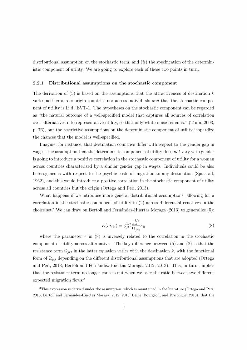
distributional assumption on the stochastic term, and (ii) the specification of the determin-
istic component of utility. We are going to explore each of these two points in turn.
2.2.1 Distributional assumptions on the stochastic component
The derivation of (5) is based on the assumptions that the attractiveness of destination k
varies neither across origin countries nor across individuals and that the stochastic compo-
nent of utility is i.i.d. EVT-1. The hypotheses on the stochastic component can be regarded
as “the natural outcome of a well-specified model that captures all sources of correlation
over alternatives into representative utility, so that only white noise remains.” (Train, 2003,
p. 76), but the restrictive assumptions on the deterministic component of utility jeopardize
the chances that the model is well-specified.
Imagine, for instance, that destination countries differ with respect to the gender gap in
wages: the assumption that the deterministic component of utility does not vary with gender
is going to introduce a positive correlation in the stochastic component of utility for a woman
across countries characterized by a similar gender gap in wages. Individuals could be also
heterogeneous with respect to the psychic costs of migration to any destination (Sjaastad,
1962), and this would introduce a positive correlation in the stochastic component of utility
across all countries but the origin (Ortega and Peri, 2013).
What happens if we introduce more general distributional assumptions, allowing for a
correlation in the stochastic component of utility in (2) across different alternatives in the
choice set? We can draw on Bertoli and Fernandez-Huertas Moraga (2013) to generalize (5):
E(mjkt) = φ1/τjkt
y1/τkt
Ωjktsjt (8)
where the parameter τ in (8) is inversely related to the correlation in the stochastic
component of utility across alternatives. The key difference between (5) and (8) is that the
resistance term Ωjkt in the latter equation varies with the destination k, with the functional
form of Ωjkt depending on the different distributional assumptions that are adopted (Ortega
and Peri, 2013; Bertoli and Fernandez-Huertas Moraga, 2012, 2013). This, in turn, implies
that the resistance term no longer cancels out when we take the ratio between two different
expected migration flows:3
3This expression is derived under the assumption, which is maintained in the literature (Ortega and Peri,
2013; Bertoli and Fernandez-Huertas Moraga, 2012, 2013; Beine, Bourgeon, and Bricongne, 2013), that the
5
E(mjkt)
E(mjjt)= φ1/τ
jkt
y1/τkt
yjt
Ωjjt
Ωjkt(9)
More general distributional assumptions, which are more consistent with the constraints
imposed on the specification of the deterministic component of utility, are no longer consis-
tent with the independence from irrelevant alternatives property: specifically, an increase in
the attractiveness of a destination that is perceived as a close substitute to k, will reduce
E(mjkt) more than E(mjjt) (Bertoli, Fernandez-Huertas Moraga, and Ortega, 2013), thus
inducing a decline in (9). This, in turn, questions the long-standing tradition in the migra-
tion literature of estimating the determinants of bilateral migration rates as a function of
the attractiveness of j and k only (Hanson, 2010).
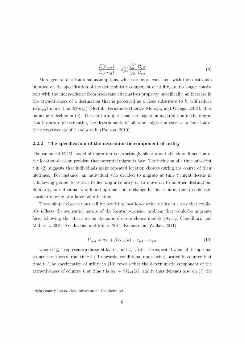
2.2.2 The specification of the deterministic component of utility
The canonical RUM model of migration is surprisingly silent about the time dimension of
the location-decision problem that potential migrants face. The inclusion of a time subscript
t in (2) suggests that individuals make repeated location choices during the course of their
lifetimes. For instance, an individual who decided to migrate at time t might decide in
a following period to return to her origin country or to move on to another destination.
Similarly, an individual who found optimal not to change her location at time t could still
consider moving at a later point in time.
These simple observations call for rewriting location-specific utility in a way that explic-
itly reflects the sequential nature of the location-decision problem that would-be migrants
face, following the literature on dynamic discrete choice models (Artuc, Chaudhuri, and
McLaren, 2010; Arcidiacono and Miller, 2011; Kennan and Walker, 2011):
Uijkt = wkt + βVt+1(k)− cjkt + ijkt (10)
where β ≤ 1 represents a discount factor, and Vt+1(k) is the expected value of the optimal
sequence of moves from time t+ 1 onwards, conditional upon being located in country k at
time t. The specification of utility in (10) reveals that the deterministic component of the
attractiveness of country k at time t is wkt + βVt+1(k), and it thus depends also on (i) the
origin country has no close substitute in the choice set.
6
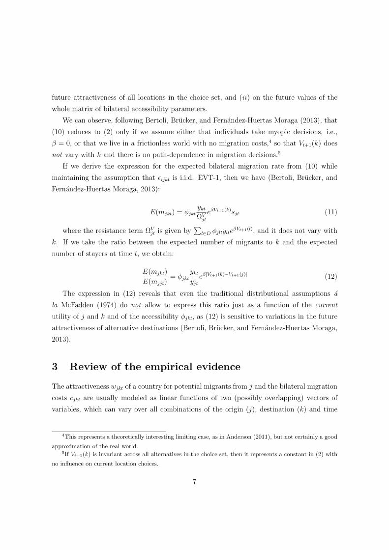
future attractiveness of all locations in the choice set, and (ii) on the future values of the
whole matrix of bilateral accessibility parameters.
We can observe, following Bertoli, Brucker, and Fernandez-Huertas Moraga (2013), that
(10) reduces to (2) only if we assume either that individuals take myopic decisions, i.e.,
β = 0, or that we live in a frictionless world with no migration costs,4 so that Vt+1(k) does
not vary with k and there is no path-dependence in migration decisions.5
If we derive the expression for the expected bilateral migration rate from (10) while
maintaining the assumption that ijkt is i.i.d. EVT-1, then we have (Bertoli, Brucker, and
Fernandez-Huertas Moraga, 2013):
E(mjkt) = φjktyktΩV
jt
eβVt+1(k)sjt (11)
where the resistance term ΩVjt is given by
l∈D φjltylteβVt+1(l), and it does not vary with
k. If we take the ratio between the expected number of migrants to k and the expected
number of stayers at time t, we obtain:
E(mjkt)
E(mjjt)= φjkt
yktyjt
eβ[Vt+1(k)−Vt+1(j)] (12)
The expression in (12) reveals that even the traditional distributional assumptions a
la McFadden (1974) do not allow to express this ratio just as a function of the current
utility of j and k and of the accessibility φjkt, as (12) is sensitive to variations in the future
attractiveness of alternative destinations (Bertoli, Brucker, and Fernandez-Huertas Moraga,
2013).
3 Review of the empirical evidence
The attractiveness wjkt of a country for potential migrants from j and the bilateral migration
costs cjkt are usually modeled as linear functions of two (possibly overlapping) vectors of
variables, which can vary over all combinations of the origin (j), destination (k) and time
4This represents a theoretically interesting limiting case, as in Anderson (2011), but not certainly a good
approximation of the real world.5If Vt+1(k) is invariant across all alternatives in the choice set, then it represents a constant in (2) with
no influence on current location choices.
7
(t) dimension. We provide a review of the existing empirical evidence on the determinants
of international migration flows derived from the estimation of gravity models.
3.1 Origin or destination-specific factors
3.1.1 Income
A key determinant of the attractiveness wkt of each location is represented by the level of
income per capita that characterizes each potential destination. A RUM-based model of
migration does not impose any constraint on the functional form of the relationship be-
tween income per capita and the deterministic component of location-specific utility in (2).
Grogger and Hanson (2011) favor a specification where wkt depends linearly on income per
capita, while other papers in the literature opt for a logarithmic specification (Mayda, 2010;
McKenzie, Theoharides, and Yang, 2013; Bertoli, Fernandez-Huertas Moraga, and Ortega,
2013; Bertoli and Fernandez-Huertas Moraga, 2013; Ortega and Peri, 2013). The literature
generally assumes that the income prospects of potential migrants from all origins can be
measured through GDP per capita at destination,6 thus mostly imposing the assumption of a
common trend in migrants’ earnings at destination, with Bertoli and Fernandez-Huertas Mor-
aga (2013) representing an exception in this respect, and also minimizing the concerns about
reverse causality. Refinements have been proposed by Grogger and Hanson (2011), which ap-
ply country-specific income tax schedules to obtain measures of post-tax earnings, Grogger
and Hanson (2011) and Belot and Hatton (2012), which recover education-specific earn-
ings, and by Beine, Bourgeon, and Bricongne (2013), which focus on wages rather than on
earnings. The empirical evidence points to a robust positive relationship between income
per capita and location-specific utility, with variations in earnings at destination that exert
a stronger influence on the bilateral migration rate than identical proportional variations
at origin in estimates that are consistent with departures from the standard distributional
assumptions (Bertoli, Fernandez-Huertas Moraga, and Ortega, 2013).
3.1.2 Credit constraints
The canonical RUM model of migration with distributional assumptions a la McFadden
(1974) implies that a simultaneous variation in the (logarithm of) income per capita at
6We have relied on this common practice for the derivation of (5).
8
origin and at destination that leaves the differential between the two countries unchanged
does not influence the bilateral migration rate. Such a perfect symmetry can disappear if
we consider that potential migrants might face credit constraints that hinder their location
choices. Credit constraints can be accommodated into the model by assuming that bilateral
migration costs cjkt are negatively correlated with income at origin, and hence with wjjt. If
the dependency of bilateral migration costs on economic conditions at origin is not properly
controlled for, then an increase in incomes at origin would reduce the bilateral migration rate
less than an identical decrease at destination, and it might even expand the scale of bilateral
migration flows. The role of credit constraints has thus been captured either through the
inclusion higher-order terms of income at origin (Vogler and Rotte, 2000; Clark, Hatton, and
Williamson, 2007; Mayda, 2010), controlling for the incidence of poverty at origin (Belot
and Hatton, 2012) or splitting the sample as a function of income at origin (Ortega and
Peri, 2013). The econometric evidence provided by Vogler and Rotte (2000), Clark, Hatton,
and Williamson (2007) and Belot and Hatton (2012) suggests that credit constraints do
hinder observed international migration flows, blurring the effect of income if not properly
controlled for (Belot and Hatton, 2012).
3.1.3 Expectations
The sequential model of migration that we summarized in Section 2.2.2 implies that the cur-
rent bilateral migration rate depends on the expectations about the evolution of economic
conditions in all countries belonging to the choice set. Bertoli, Brucker, and Fernandez-
Huertas Moraga (2013) have recently provided econometric evidence on the role of expecta-
tions in driving bilateral migration flows. Specifically, they have shown that the fluctuations
in the yields on 10-year government bonds in European countries are significantly associated
with the country-specific share of respondents that are concerned about the evolution of per-
sonal job prospects in the Eurobarometer surveys. The analysis of the bilateral migration
flows to Germany between 2006 and 2012 conducted by Bertoli, Brucker, and Fernandez-
Huertas Moraga (2013) reveals that the elasticity of the migration rate with respect to the
yields of 10-year bonds at origin stands at 0.14, so that changes in expectations can influ-
ence current migration decisions even after controlling for traditional determinants of the
attractiveness of a country. Furthermore, when changes in the future attractiveness of alter-
native destinations are not controlled for, the estimates of the effect of current labor market
9
conditions at origin are significantly biased.
3.1.4 General immigration policies
Migration costs cjkt can be, at least partly, policy-induced. The immigration policies adopted
by the country of destination can be either general, i.e., addressed to all countries of origin,
or bilateral. We analyze here the existing evidence on general immigration policies, while
bilateral policies are dealt with in Section 3.2.2. Limited progress has been made on the
measurement of policy-induced migration costs compared to the existing data sources on
tariff and non-tariff barriers to trade (see Anderson and van Wincoop, 2004). Early at-
tempts have been provided by Clark, Hatton, and Williamson (2007), Mayda (2010) and
Ortega and Peri (2013). In particular, Ortega and Peri (2013) analyze the role of general
immigration policies in a micro-founded gravity model as in (8). The key policy measure,
which represents an extension of Mayda (2010), refers to an index of entry tightness over
the period 1980-2006 for 15 OECD countries. This index, which is not comparable across
destinations, is negatively associated with the scale of incoming migration flows in estimates
where between-destination variability is not used for identification. An attempt to build
measures of immigration policies that are comparable both between countries and over time
is represented by the on-going IMPALA project, which aims at building a database based on
immigration laws in the 26 most important destination countries.7 While progress has been
made on this front, we are nevertheless very far away from a full-fledged database usable in
the estimation of gravity models. In the absence of satisfying measures on immigration, one
can nevertheless make use of the panel dimension and include dkt fixed effects that control
for the influence of general immigration policies, as in Beine, Docquier, and Ozden (2011),
Bertoli and Fernandez-Huertas Moraga (2012) and Beine and Parsons (2012).
3.1.5 Unemployment rate
The unemployment rate figures prominently in the seminal analysis of internal migration
decisions by Harris and Todaro (1970), but little evidence on its impact on international mi-
gration flows has been, to date, gathered, with Beine, Bourgeon, and Bricongne (2013) and
Bertoli, Brucker, and Fernandez-Huertas Moraga (2013) representing two recent exceptions.
7The general presentation of the project and an analysis of preliminary data are exposed in Burgoon,
An increase in the unemployment rate can reduce the attractiveness wkt of a potential des-
tination, and supportive evidence in this direction has been provided by Beine, Bourgeon,
and Bricongne (2013) and Bertoli, Brucker, and Fernandez-Huertas Moraga (2013). The
effect of an increase in the unemployment rate on the decision to migrate can be mitigated
by the existence of unemployment benefits: as recently arrived immigrants are not eligible
for these benefits, then the bilateral migration flow mjkt could be more sensitive to varia-
tions in unemployment in the destination k rather than in the origin j. This differential
sensitivity could be reinforced if an increase in unemployment at origin tightens the credit
constraints discussed in Section 3.1.2. Beine, Bourgeon, and Bricongne (2013) find support
for a negative impact of unemployment at origin on top of its direct migration-enhancing
role.8
3.1.6 Environmental factors
There is a very substantial empirical literature on the impact of environmental factors on
international migration. Environmental factors include a large set of natural factors in which
pure climatic factors represent only a subset. Environmental factors include pure climatic
factors such as rainfalls and temperatures. They also include natural disasters whose climatic
origin might be subject to discussion. Hurricanes or extreme floods are supposed to be related
to climate since their frequencies and magnitudes have clearly increased along with climate
change. The connection is much less obvious for other events such as earthquakes or insect
invasion.
The channels through which climatic factors spur emigration are many-fold, with four of
them mostly considered in the literature. First, negative climatic shocks decrease income at
origin, which influences wjt, through a decline in wages or a rise in the employment rate.
Second, the shocks might increase bilateral migration costs cjkt if they destroy assets, thus
making credit constraints more binding. Third, detrimental climatic shocks tend to decrease
attractiveness at origin independently from income (for instance, because of an increase in
morbidity), which in turn leads to emigration. A fourth channel can be called the volatility
channel: if climatic conditions become more volatile, then this can increase the volatility of
8Nevertheless, as the authors emphasized, the results should be taken with caution, since they are
obtained from a specification that departs from the theory, as it does not include origin-time dummies (see
Section 4.5 on this).
11
wjt, inducing risk-averse people to opt for migration.
Most of the empirical literature linking climatic factors and migration has operated in
models of monodic migration flows, as opposed to dyadic flows which is the basic unit
of analysis in gravity frameworks. The main bulk of papers have also focused on South-
North migration, i.e., emigration from less developed countries in the face of adverse climatic
disturbances. Lilleor and Van den Broeck (2011) and Millock (2013) provide good surveys of
this extensive literature. In general, the literature finds much evidence in favor of a strong
labor market channel but also finds compelling evidence that in some cases the liquidity
channel is at work. In contrast with this extensive literature on climatic shocks, there is
much less work relying on gravity models of migration. Beine and Parsons (2012) represent a
noticeable exception. Their use of a longitudinal multiple-origin multiple-destination dataset
allows to include a rich combination of fixed effects for capturing unobservable factors. In
particular, the inclusion of dkt fixed effects allows to control for general immigration policies.
This is particularly important since the main effects of climatic factors are supposed to
operate in South-North (and South-South) international migration. Immigration policies
in developed countries are expected to be quite restrictive for prospective migrants coming
from less developed countries, the areas that are the most adversely affected by climatic
shocks. Beine and Parsons (2012) find support in favour of a strong labour market channel
in South-North migration, but reject the so-called amenity channel.
3.2 Dyadic factors
The dyadic factors that influence migration costs cjkt can be both time-invariant, such as lin-
guistic and cultural proximity, and time-varying factors, such as bilateral migration policies
and networks. We cover these factors in reverse order.
3.2.1 Networks
An extensive literature has been devoted to the role of migration networks on the magnitude
and the shape of bilateral migration flows.9 The role of networks have been analyzed in micro-
founded gravity models such as (4); while there are obviously econometric challenges to be
overcome in order to correctly estimate that effect, the few existing papers based on structural
9For classical examples of a microeconomic analyses of the role of migrants’ networks, which are not
covered here, see Munshi (2003) and McKenzie and Rapoport (2010).
12
gravity models (Beine, Docquier, and Ozden, 2011; Bertoli and Fernandez-Huertas Moraga,
2012; Beine and Parsons, 2012) come up with quite consensual results: a 10 percent increase
in the bilateral migration stock leads to a four percent increase in the bilateral migration
flow over the next ten years. This elasticity increases to 0.7 when we restrict our attention
to migration to OECD destinations, and it is higher for low-educated than for high-educated
migrants, thus lowering the average level of education of the migrants.10 We can also notice
that the share of explained variability by structural gravity models of migration is in the
range of 50 to 70 percent, and at least one third of that proportion can be ascribed to the
network effect. Failure to account for networks can lead to some an omitted variable bias.
This is well illustrated by the role of colonial links. Once accounted for the network effect,
regressions based on micro-founded gravity models such as (4) fail to find any remaining role
for colonial links.
3.2.2 Bilateral immigration policies
Two broad types of measures capturing bilateral policies have been used in the literature.
First, one can capture the prevalence of bilateral agreements between countries: for instance,
Grogger and Hanson (2011) and Beine, Bourgeon, and Bricongne (2013) find larger bilateral
migration flows when both the origin and the destination country are signatories of the
Schengen agreement,11 and Beine, Bourgeon, and Bricongne (2013) provide similar evidence
for the bilateral agreements between OECD countries and collected by the IOM. The second
main measure relates to bilateral visa policies. Visa waivers, which do not belong de jure
to the legal framework that regulates immigrants’ admission at destination, can facilitate
the legal entry of migrants, thus reducing the bilateral migration costs cjkt, and also reflect
a preferential treatment at the dyadic level. Bertoli and Fernandez-Huertas Moraga (2013)
provide evidence on the impact of visa waivers on bilateral migration flows to Spain in a
specification that uses high-frequency migration data and controls for time-varying bilateral
unobservables, including cultural proximity, through a rich structure of fixed effects. Similar
evidence in provided by Bertoli and Fernandez-Huertas Moraga (2012) and Beine and Parsons
10This aggregate effect can be decomposed into an assimilation channel, e.g., decrease in policy unrelated
migration costs such as information and adaptation costs, and into a policy-related effect, with Beine, Ragot,
and Noel (2013) proposing an identification strategy to disentangle the two channels.11Ortega and Peri (2013) provide similar evidence, but the Schengen dummy is not bilateral, as it is based
only on the signatory status of the destination country.
13
(2012), with this latter paper using longitudinal data on bilateral visa policies collected by
the DEMIG project at Oxford University.
3.2.3 Linguistic and cultural proximity
As in the trade literature, the most important time-invariant dyadic components of bilateral
migration costs cjkt are bilateral distance, colonial links, linguistic and cultural proximity.
Bilateral distance does not require much explanation. As discussed above, the influence of
colonial links can be indirectly captured through the network effect. This is in contrast
with linguistic proximity that exerts some additional effect beyond its influence through
networks. Most of the analyzes based on gravity equations and covered here capture the role
of languages either through the use of dummies for the existence of a common (official or
spoken) language between j and k, or through some simple measures of linguistic proximity.
More elaborated indicators of linguistic proximity have been nevertheless used in gravity
equations: Belot and Ederveen (2012) and Adsera and Plytikova (2012) employ proximity
indicators based on family trees established by linguists. This captures the fact that Italian
prospective migrants can (more) easily become proficient in the local language in either
Spain or France than in Japan, although Italy does not share a common language with none
of these three destinations. Cultural proximity is a more elusive concept than linguistic
proximity. Belot and Ederveen (2012) use particular measures capturing, at least partly,
this dimension: these are variables describing bilateral religious distance and survey-based
measures capturing the cultural orientation of countries, both fostering bilateral migration
flows.
4 Challenges for the estimation
4.1 What is the origin of the migrant?
An international migrant can be defined as “any person who changes his or her country of
usual residence” (United Nations, 1998), but the measures of the bilateral gross migration
flows mjkt often departs from this definition. Specifically, the origin j can be defined as (i)
the country of birth, (ii) the country of citizenship, or (iii) the country of last residence of the
migrant. These three criteria partly overlap, but do not coincide, because of naturalizations
14
and of the possibility of repeated migration episodes. Existing data sources rarely provide
information on more than one of the criteria (i)-(iii), so that, say, data on bilateral migration
flows based on the country of birth j aggregate the migration decisions of individuals who
are citizens and that resided in countries other than j. The adoption of one of these three
criteria, which are often data-driven, presents some advantages and limitations. For instance,
some dyadic determinants of migration costs, such as visa waivers, depends on citizenship,
while linguistic proximity could depend more closely on the country of birth and economic
conditions in the country of last residence could shape the incentives to move.
4.2 The empirical counterpart for the log odds
The RUM model analyzed in Section 2 implies that the logarithm of the odds of migrating to
country k over staying in country j can be expressed as a linear function of the differential in
the deterministic component of utility associated to the two countries. Ideally, the empirical
counterpart of the log odds would be represented by the ratio between the gross flow of
migrants from j to k observed on a certain time period12 over the number of individuals who
remained in j throughout the period.
As far as the numerator of this ratio is concerned, gross flows have been used by Mayda
(2010), Ortega and Peri (2013), Bertoli and Fernandez-Huertas Moraga (2013), McKenzie,
Theoharides, and Yang (2013) and Bertoli, Brucker, and Fernandez-Huertas Moraga (2013).
Other papers have used a proxy for the gross flows represented by the variations in migra-
tion stocks (Beine, Docquier, and Ozden, 2011; Bertoli and Fernandez-Huertas Moraga, 2012;
Beine and Parsons, 2012). A limitation is that variations in stocks differ from gross flows as
they are also influenced return migration, migration to third countries, deaths, and natural-
izations (if the definition of immigrants is based on citizenship) and births (if the country of
destination adopts the jus sanguinis). Furthermore, while mjkt is by definition nonnegative,
variations in stocks can take negative values, which have been excluded from the sample
(Beine, Docquier, and Ozden, 2011), set to zero (Bertoli and Fernandez-Huertas Moraga,
2012), or added to the proxy for the flow from k to j (Beine and Parsons, 2012). Grogger
and Hanson (2011) and Llull (2011) have used stocks for the numerator, but this choice
12The length of the time period also represents a crucial analytical choice: longer time periods, such as a
decade, create problems for the (implicit) assumption in the RUM model that the deterministic component
of location-specific utility in (2) does not vary within the period.
15
creates a tension with the underlying micro-foundation of the gravity equation.
For the denominator, the size of population at origin has been used (Bertoli and Fernandez-
Huertas Moraga, 2012), possibly restricted to certain age cohorts (Bertoli, Brucker, and
Fernandez-Huertas Moraga, 2013), but this also includes immigrants, or the number of na-
tives at origin (Beine and Parsons, 2012), which represents a superior alternative as it only
includes stayers and returnees. A convenient alternative, for datasets that include multiple
destinations, is represented by the inclusion of origin-time dummies djt that control for the
denominator of the dependent variable, although this choice comes at a cost that is discussed
in Section 4.4 below.
4.3 Multilateral resistance to migration
Bertoli and Fernandez-Huertas Moraga (2013) define multilateral resistance to migration as
the confounding influence that the attractiveness of alternative destinations exerts on the
determinants of bilateral migration rates. Section 2 follows Bertoli, Brucker, and Fernandez-
Huertas Moraga (2013) and shows how multilateral resistance to migration can arise either
from more general distributional assumptions on the stochastic component in (2), or from
explicitly accounting for the sequential nature of migration decisions.
Ignoring the term Ωjkt in (9) generates biases in the estimation of relevant coefficients
of the determinants of migration. For example, both Bertoli and Fernandez-Huertas Mor-
aga (2013) and Bertoli, Brucker, and Fernandez-Huertas Moraga (2013) find that the effect
of economic conditions at origin on migration rates is overestimated when the influence of
alternative destinations is ignored. The reason is that economic conditions are correlated be-
tween origins and alternative destinations, both over time and space. Thus, when alternative
destinations are disregarded, the origin term wjt picks up both its own effect and the effect
of these alternative destinations that goes through Ωjkt. If, say, migration between Ecuador
and Spain increased because of worsening economic conditions in Ecuador and worsening
economic conditions in Ecuador were correlated with worsening economic conditions in, say,
Chile, then estimates that disregard Ωjkt would attribute all of the increase in the bilateral
migration rate to Spain to the worsening of economic conditions in Ecuador. The scope for
large biases is even more pronounced when migration policies are considered. Given that
migration policies tend to be coordinated among destination countries, e.g., the European
Union, it is not surprising that studies controlling for multilateral resistance to migration
16
tend to find much larger policy effects than studies that do not control at all (Bertoli and
Fernandez-Huertas Moraga, 2012, 2013). This happens even in the case of empirical strate-
gies that only control for Ωjkt under less general distributional assumptions (Ortega and
Peri, 2013; Beine and Parsons, 2012).
Different authors have proposed different strategies to control for Ωjkt. When the panel
and longitudinal dimension of the dataset are large enough, the resistance term nicely con-
forms with the structure of the CCE estimator proposed by Pesaran (2006). This is the
methodology used by Bertoli and Fernandez-Huertas Moraga (2013) and Bertoli, Brucker,
and Fernandez-Huertas Moraga (2013) and it has the additional advantage of being robust
even in the presence of residual cross-sectional dependence in the data (Pesaran and Tosetti,
2011). Using less data-demanding approaches, Ortega and Peri (2013) control for the mul-
tilateral resistance to migration that is induced by an heterogeneity in the preference for
migration, so that Ωjkt does not vary across destinations k except the origin j itself. This
empirically corresponds to estimating the gravity equation with origin-year dummies djt.
Bertoli and Fernandez-Huertas Moraga (2012) go one step further, and assume that poten-
tial migrants are heterogeneous in their preferences towards subsets (nests) of destination.
With their cross-sectional data, this specific Ωjkt can be controlled for with origin-nest dum-
mies. Finally, Beine and Parsons (2012) use destination-year dummies dkt, which allows
them to partly control for the dynamic resistance terms introduced in Section 2.2.2.
Whether any of these alternative approaches or even the classical one that ignores mul-
tilateral resistance to migration altogether is enough to generate unbiased estimates is ulti-
mately an empirical question. Following the theory, one necessary condition for the estimates
to be RUM-consistent is to make sure that their residuals are cross-sectionally independent.
In this sense, Bertoli and Fernandez-Huertas Moraga (2012) propose adapting the CD test by
Pesaran (2004) to make sure there are no remaining signs of correlation across destinations
for different origins so that Ωjkt is properly controlled for.
4.4 Estimates and structural parameters of the RUM model
Using a micro-founded model to estimate the determinants of aggregate migration rates can
have some costs in terms of the interpretation of the coefficients. Whenever the existence
of multilateral resistance to migration forces the researcher to depart from the classical
framework, the parameters of the different distributions that can be used to model the
17
dependence of bilateral decisions on unobserved factors can impede the exact identification
of the relevant elasticities of migration flows with respect to their determinants.
Bertoli and Fernandez-Huertas Moraga (2012) provide a very simple example. In their
model, individual utility in each location depends on origin-destination factors plus an
individual-specific error term that is allowed to be correlated within different nests of desti-
nations. This correlation is the one that generates multilateral resistance to migration when
individual decisions are aggregated at the origin-level for estimation purposes. In particular,
Bertoli and Fernandez-Huertas Moraga (2012) write the bilateral migration flow between
two countries as a function of bilateral factors, origin country fixed effects and an origin-nest
fixed effect, which embodies the effect of the characteristics of countries that are perceived
as close substitutes to the destination by origin-country individuals. The problem is that the
bilateral factors also belong to this origin-nest term and they belong to it with a particular
functional form. In the simple case of a nested logit model, this means that the elasticity of
migration flows with respect to bilateral factors will depend on the dissimilarity parameter
τ in (8).
The type of variability that Bertoli and Fernandez-Huertas Moraga (2012) exploit for
identification does not allow them to separately identify τ . The only thing they can do is
to take advantage from the fact that τ ∈ (0, 1]. and that the elasticities are monotonic
functions of τ . This allows them to construct upper and lower bounds for the elasticities
of interest. These bounds are bilateral since the elasticities do not only depend on fixed
parameters but also on the shares of the population who migrate or not between countries
and on the substitutability of the destination countries with alternative destinations for each
origin. Due to this dependence, the tightness of the bounds will hinge on the particular
origin-destination pair. In general, bounds will be tighter whenever a given destination does
not have many alternatives that are considered substitutable.
The inclusion of origin-time dummies djt among the regressors13 implies that the esti-
mates are consistent with a RUM model that is not based on distributional assumptions a la
McFadden (1974), so that the fundamental uncertainty in the estimated elasticities should
always be considered.
13See, for instance, Beine, Docquier, and Ozden (2011), McKenzie, Theoharides, and Yang (2013) and
Ortega and Peri (2013) for different justifications for the inclusion of these dummies.
18
4.5 Estimation in logs or in levels
The pseudo-gravity model of migration derived from the underlying RUM model can be
estimated using as the dependent variable either the level of the bilateral gross migration
flow in (7), or the empirical counterpart qjkt of the ratio of choice probabilities in (6). This
second option requires estimating, through OLS, the following equation:
qjkt = ln(φjkt) + ln(ykt)− ln(yjt) + ln
ηjktηjjt
(13)
Santos Silva and Tenreyro (2006) made the point that the assumption that E(ηjkt) = 1
does not imply that E [ln (ηjkt/ηjjt)] = 0, and that the heteroskedasticity of ηjkt entails that
the expected value of ln (ηjkt/ηjjt) in (13) will be a function of the value of the regressors,
thus making OLS estimates biased and inconsistent. This, in turn, calls for relying on the
bilateral gross migration flow as the dependent variable as in (7), and estimating the model
with Poisson Pseudo-Maximum Likelihood, PPML. This choice requires to always include
origin-time dummies among the regressors, to control for the resistance term Ωjt and for the
number of potential migrants sjt, while the inclusion of these dummies is, as discussed in
Section 2.2, not strictly necessary when estimating (13).14
The choice of the estimation technique for the gravity model of migration confronts the
researcher with an important trade-off: the reliance on linear models through the logarith-
mic transformation widens the menu of estimators that can be adopted, as discussed in
Section 4.2, to deal with multilateral resistance to migration, while Bertoli and Fernandez-
Huertas Moraga (2012) represents, to date, the only paper that deals with multilateral resis-
tance to migration with PPML under more general distributional assumptions than Ortega
and Peri (2013)15 through a richer structure of fixed effects.
4.5.1 Presence of zeros in the data
The case for relying on PPML is strengthened when the dependent variable takes zero values,
as Santos Silva and Tenreyro (2011) have shown that this estimator performs well even in
the presence of a large share of zeros in the data. An alternative with linear models is
14The estimation of (13) with the CCE estimator proposed by Bertoli and Fernandez-Huertas Moraga
(2013) allows to deal with heteroskedastic disturbances in (7).15PPML estimates are always consistent with heterogeneity in the propensity to migrate when origin-time
dummies are included.
19
represented by a two-stage selection model a la Heckman adopted by Beine, Docquier, and
Ozden (2011). Identification is improved by the availability of a variable that can be excluded
from the second stage equation, but credible exclusion restrictions are hard to find with data
that have a longitudinal dimension.
4.6 Omitted variables and instrumentation
The existence of omitted variables drives a wedge between the deterministic component of
utility wkt − cjkt in (2) and its empirical counterpart. This calls for estimation approaches
that are consistent with more general distributional assumptions on ijkt in (2), as omitted
variables end up in the error term and can give rise to a correlation in the stochastic com-
ponent of utility across destinations. Controlling for multilateral resistance to migration can
make instrumentation unnecessary as long as the endogeneity problem is not due to reverse
causality or as long as the resistance terms capture a big part of the omitted factors.
Second, if the two above conditions do not apply, instrumentation of some of the key
variables might be needed. Three issues arise in that respect. The first issue is of course
to find an instrument that is correlated with the key variable of interest and not correlated
with the bilateral flows. The existence of such an instrument is subject to discussion. The
presence of serial correlation in the error term of specification (4) invalidates the use of
internal instruments, i.e., past bilateral flows in a panel set-up. This means that external
instruments should be favored. For instance, networks are clearly endogenous in equation
(4). Endogeneity might come from omitted variables, e.g., networks are correlated with
unobserved cultural proximity, but in some cases also from some kind of reverse causality,
e.g., flows are computed from stocks which is the macro proxy of networks. To that purpose,
Beine, Docquier, and Ozden (2011) use the existence of guest worker programs at destination
(that came to an end in the late 1960s) to instrument for networks. Another example is
provided by Beine, Ragot, and Noel (2013), who instrument education fees affecting the
migration of international students with the share of public universities in the destination
country.
The second issue is that instrumentation preferably needs to take place in a Poisson re-
gression set-up, as discussed in Section 4.5 above. To that purpose, Tenreyro (2007) proposes
to combine PPML estimation and instrumentation using a GMM-type of estimator. Beine,
Ragot, and Noel (2013) implement that approach in the context of international migration
20
of students. Nevertheless, the estimation might face in practice important problems of con-
vergence towards the optimal values of the estimates and one cannot rule out the existence
of local maxima in the support of admissible values for the key parameters. Finally, if multi-
lateral resistance to migration is still an issue, the instrumentation procedure should ideally
account for it, both in the first and in the second stage.
5 Conclusions
The use of bilateral data for the analysis of international migration is at the same time a
blessing and a curse. It is a blessing since the dyadic dimension of the data allows to analyze
many previously unaddressed questions of the literature. The development and the use of
country-pair flows and stocks of international migration allow to identify many important
determinants such as the network effect, the role of poverty constraints or the impact of
cultural links between countries. This paper reviews some of the recent studies using this
type of data in order to identify the important factors affecting international migration flows.
Our review demonstrates that significant efforts have been conducted by many scholars and
that overall we have a much better knowledge of the important determinants.
Still, the use of bilateral data is also a curse. The methodological challenges that are
implied by the use of this type of data are numerous and our paper covers some of the most
important ones. We show that a good connection with the underlying micro foundations
is desirable, something very much in line with the literature on trade. The reference to
the underlying theoretical frameworks such as the RUM model clarifies the need to account
for important issues such as multilateral resistance to migration. In turns this has strong
implications for the econometric estimation methods that need to be used. Additional issues
such as the presence of many zero observations or endogeneity concerns due to ommitted
factors have also strong implications for the choice of the appropriate econometric techniques.
Fortunately, the recent evolution of the literature suggests that scholars are increasingly
aware of these challenges.
21
References
Adsera, A., and M. Plytikova (2012): “The role of language in shaping international
migration,” Norface Discussion Paper Series No. 2012014, London.
Anderson, J. (2011): “The Gravity Model,” Annual Review in Economics, 3(1), 133–160.
Arcidiacono, P., and R. A. Miller (2011): “Conditional Choice Probability Estima-
tion of Dynamic Discrete Choice Models With Unobserved Heterogeneity,” Econometrica,
79(6), 1823–1867.
Artuc, E., S. Chaudhuri, and J. McLaren (2010): “Trade Shocks and Labor Adjust-
ment: A Structural Empirical Approach,” American Economic Review, 100(3), 1008–1045.
Beine, M., P. Bourgeon, and J.-C. Bricongne (2013): “Aggregate Fluctuations and
International Migration,” CESifo Working Paper No. 4379, Munich.
Beine, M., F. Docquier, and C. Ozden (2011): “Diasporas,” Journal of Development
Economics, 95(1), 30–41.
Beine, M., and C. Parsons (2012): “Climatic factors as determinants of International
Migration,” CESifo Working Paper No. 3747, Munich.
Beine, M., L. Ragot, and R. Noel (2013): “The Determinants of International Mobility
of Students,” Economics of Education Review, forthcoming.
Belot, M., and S. Ederveen (2012): “Cultural barriers in migration between OECD
countries,” Journal of Population Economics, 25(3), 1077–1105.
Belot, M., and T. Hatton (2012): “Skill Selection and Immigration in OECD Coun-
tries,” Scandinavian Journal of Economics, 114(4), 1105–1128.
Bertoli, S., H. Brucker, and J. Fernandez-Huertas Moraga (2013): “The Eu-
ropean Crisis and Migration to Germany: Expectations and the Diversion of Migration
Flows,” Working Paper No. 2013/21, CERDI, University of Auvergne.
Bertoli, S., and J. Fernandez-Huertas Moraga (2012): “Visa Policies, Networks
and the Cliff at the Border,” IZA Discussion Paper No. 7094, Bonn.
22
(2013): “Multilateral Resistance to Migration,” Journal of Development Economics,
102, 79–100.
Bertoli, S., J. Fernandez-Huertas Moraga, and F. Ortega (2013): “Crossing the
Border: Self-Selection, Earnings and Individual Migration Decisions,” Journal of Devel-
opment Economics, 101(1), 75–91.
Burgoon, B., M. Beine, A. Boucher, M. Crock, J. Gest, M. Hiscox, P. McGov-
ern, H. Rapoport, J. Schaper, and E. Thielemann (2013): “Comparing immigra-
tion policies: An overview from the IMPALA database,” Paper presented at the MAFE
meeting, San Diego.
Carey, H. C. (1858): Principles of Social Science. Philadelphia: Lippincott.
Clark, X., T. Hatton, and J. Williamson (2007): “Explaining U.S. immigration,
1971-1998,” Review of Economics and Statistics, 89(2), 359–373.
Grogger, J., and G. H. Hanson (2011): “Income maximization and the selection and
sorting of international migrants,” Journal of Development Economics, 95(1), 42–57.
Hanson, G. H. (2010): “International Migration and the Developing World,” in Hand-
book of Development Economics, ed. by D. Rodrik, and M. Rosenzweig, pp. 4363–4414.
Amsterdam: North-Holland, Volume 5.
Harris, J. R., and M. P. Todaro (1970): “Migration, Unemployment and Development:
A Two-Sector Analysis,” American Economic Review, 60(1), 126–142.
Head, K., and T. Mayer (2013): “Gravity Equations: Workhorse,Toolkit, and Cook-
book,” in Handbook of International Economics, ed. by G. Gopinath, E. Helpman, and
K. Rogoff. Elsevier, Volume 4.
Kennan, J., and J. R. Walker (2011): “The Effect of Expected Income on Individual