53
April 2009 The Method of Fundamental Solutions applied to eigenproblems in partial differential equations Pedro R. S. Antunes - CEMAT (joint work with C. Alves)
| Date post: | 19-Dec-2015 |
| Category: |
Documents |
| View: | 215 times |
| Download: | 1 times |

April 2009
The Method of Fundamental Solutions applied
to eigenproblems in partial differential equations
Pedro R. S. Antunes - CEMAT
(joint work with C. Alves)

Experimental results of resonance
Eigenvalue problem for the Laplacian
- some results and questions
Numerical solution using the Method of Fundamental Solutions (MFS)
- eigenfrequency calculation
- eigenfunction calculation
- numerical simulations with 2D and 3D domains
Hybrid method for domains with corners or cracks
Shape optimization problem
Extension to the Bilaplacian eigenvalue problem and to the eigenvalue in elastodynamics
Conclusions and future work
• Outline

Experimental results of resonance
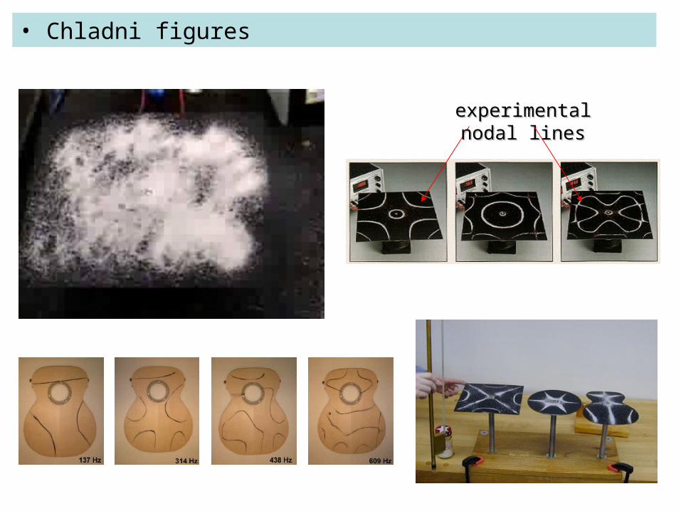
experimental nodal linesexperimental nodal lines
• Chladni figures
Eigenvalue problem for the Laplacian

Search for k (eigenfrequencies) such that there exists non null function u (eigenmodes) :
on 0uor 0
2,3d ,in 0
n
2
uRuku d
An application: Calculate the resonance frequencies and eigenmodes associated to a drum (2D) or a room (3D)
n 0
• Eigenvalue problem for the Laplacian
General results: Countable number of eigenvalues The sequence goes to infinity 1>0 1=0

Numerical methods – eigenfrequency calculation

Finite Elements, Finite Differences, Boundary Elements
Meshless Methods
Consider the rigidity matrix Ah(k).(h – discretization parameter, k – frequency)
Fixed h, search k : matrix is not invertible (eg: det(Ah(k)) = 0 )
- particular solutions - angle Green’s functions (Moler&Payne, 1968, Trefethen&Betcke, 2004)
- radial basis functions (JT Chen et al., 2002, 2003)
- method of fundamental solutions (Karageorghis, 2001; JT Chen et al., 2004; Alves&Antunes, 2005)
• Numerical methods - eigenfrequency calculation

~1
m
jjkj yxxuxu
y j
• The Method of Fundamental Solution (MFS)
Fundamental solution:
Consider the approximation
The coefficients j are calculated such that fits the boundary conditionsu~
an admissible curve

Given an open set Rd, different points and kC,
are linearly independent on .
The set is dense in L2(),
when is an admissible curve.
c
myy ,...,
1
yyxSpanxk :
)}(),...,({ 1 mkk yxyx
• Theoretical results
is not an eigenfrequency

Consider m points x1 ,…, xm collocation points (almost equally spaced)
Define m points y1 ,…, ym source points
),(2
1~ ,~/~ 1,,1 jjjjjjjjj xy nnnnn
xi yi
• Algorithm for the source points (2D)

1 2 3 4 5 6
-40
-35
-30
BesselJ zeros (exact values)
Circle:Plot of Log[g(k)]
Search for local minimum using the Golden Ratio Search
Due to the ill conditioning of the matrix g(k) is too small
• Algorithm for the eigenfrequency calculation
)()(
jy
ix
kkAm Build the matrices
Consider g(k)=|det(Am(k))| and look for the minima

m
jjkjm yxxuxu
0
)()()(~
To calculate j solve the system
0)(~, ... ,0)(~,1)(~
1
0
mxuxu
xu
Given the approximate eigenfrequency k, define
- non null solution,- null at boundary points
The extra point x0 is not on a nodal line
• Algorithm for the eigenmode calculation
x0y0
Define extra points { Cy 0
0x
{
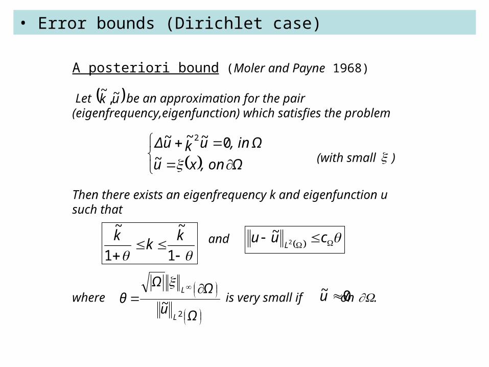
• Error bounds (Dirichlet case)
Let be an approximation for the pair (eigenfrequency,eigenfunction) which satisfies the problem
(with small )
Then there exists an eigenfrequency k and eigenfunction u such that
and
where is very small if on .
1
~
1
~k
kk
A posteriori bound (Moler and Payne 1968)
Ωu
ΩΩθ
L
L
2~
Ω, on xu
, in ΩukuΔ
~0~~~ 2
uk ~,~
cuu
L2~
0~ u

Numerical Tests (algorithm validation)

m=dimension of the matrix
m abs. error (k1) m abs. error (k2) m abs. error (k3)
30 5.7210-6 30 1.3610-6 30 1.8110-5
40 8.4210-8 40 1.6710-7 40 2.1710-7
50 7.7610-8 50 1.1110-8 50 6.9410-8
60 1.4610-9 60 1.4410-9 60 3.1710-9
m abs. error (k1) m abs. error (k2) m abs. error (k3)
30 2.3110-6 30 4.9410-6 30 5.2110-6
40 5.9110-8 40 1.2110-8 40 1.2610-7
50 1.6410-9 50 3.0110-10 50 3.2710-9
60 8.2310-11 60 9.3110-12 60 9.3510-11
m abs. error (k5) m abs. error (k5) m abs. error (k5)
20 2.1110-4 30 1.4610-5 40 1.2310-6
50 3.0610-7 60 2.5210-8 70 5.0510-9
80 3.1910-9 90 6.1910-10 100 1.8710-10
• Numerical tests (Dirichlet case) – 2D

m abs. error (k1) m abs. error (k2) m abs. error (k3)
112 1.2510-8 112 9.2110-7 112 8.5710-6
158 8.6110-12 158 1.9710-9 158 6.5310-8
212 2.1810-14 212 1.6110-13 212 9.4610-11
m abs. error (k1) m abs. error (k2) m abs. error (k3)
218 6.1310-10 218 9.2710-7 218 1.5510-6
296 3.1110-10 296 7.3110-8 296 7.0910-8
386 9.1510-12 386 5.2510-9 386 1.9510-10
m abs. error (k5) m abs. error (k5) m abs. error (k5)
226 1.3610-5 304 5.8710-6 374 7.2110-8
• Numerical tests (Dirichlet case) – 3D
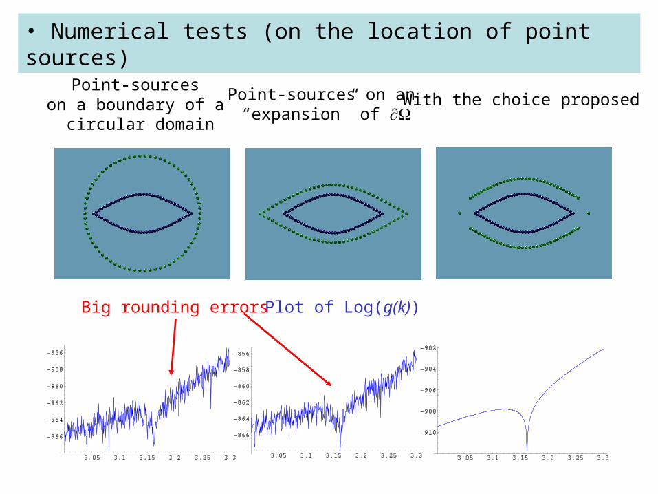
Plot of Log(g(k))
Point-sources on a boundary of a
circular domain
Point-sources on an “expansion” of
With the choice proposed
Big rounding errors
• Numerical tests (on the location of point sources)

m abs. error (k2) abs. error (k3)
60 1.1510-10 1.2510-10
70 4.1610-11 6.8310-12
80 3.3310-12 5.0310-12
1
1+10-8
k3-k2≈4.2110-8
Plot of Log(g(k)) with n=60
7.02481 7.02481 7.02481 7.02481 7.02481 7.02481 7.02481-631
-630
-629
-628
-627
-626
• Numerical tests (almost double eigenvalues)

Numerical Simulations (non trivial domains)

Plots of eigenfunctions associated to the 21th,…,24th eigenfrequencies
• Numerical Simulations

(Dirichlet and Mixed boundary conditions)
Dirichlet problem
Mixed problemDirichlet - external boundaryNeumann - internal boundary
nodal lines plot eigenmode
• Numerical Simulations

3D plots of eigenfunctions associated to three resonance frequencies
• Numerical simulations – non trivial domains 3D
Domains with corners or cracks Hybrid method
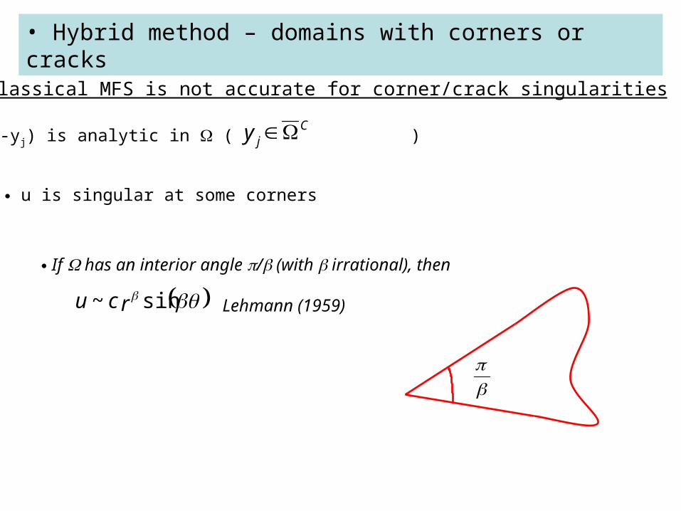
• Hybrid method – domains with corners or cracks
k(x-yj) is analytic in ( )Cjy
If has an interior angle / (with irrational), then
Lehmann (1959)
sin~ rcu
u is singular at some corners
The classical MFS is not accurate for corner/crack singularities
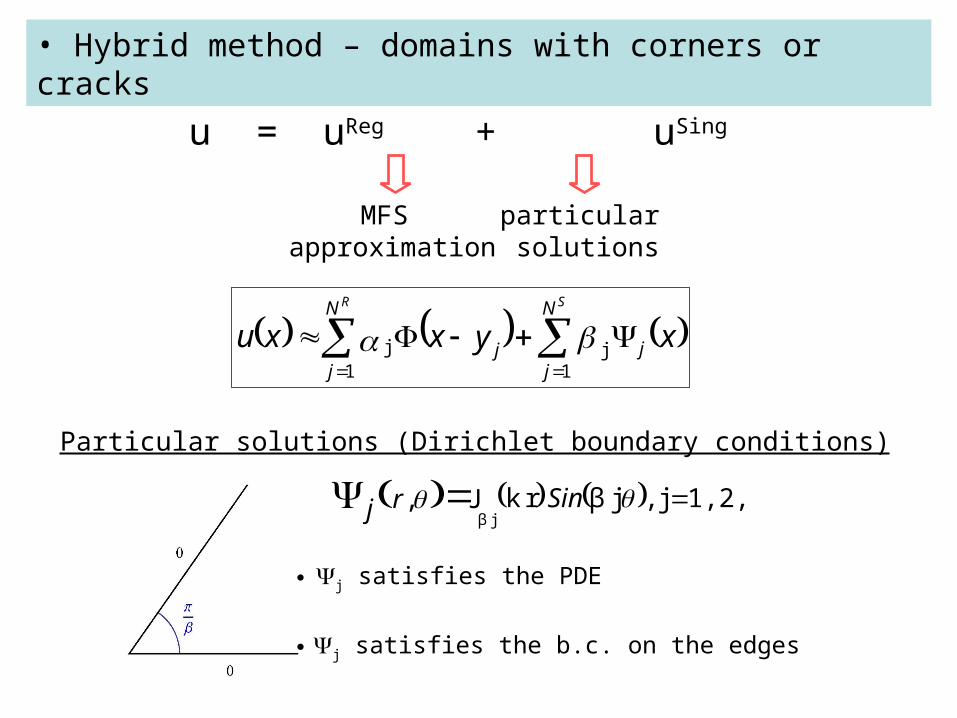
u = uReg + uSing
MFS approximation
particular solutions
1,2,...j , j β rk J,j β
Sinrj
xyxxu j
N
jj
N
j
SR
1
j1
j
• Hybrid method – domains with corners or cracks
Particular solutions (Dirichlet boundary conditions)
j satisfies the PDE
j satisfies the b.c. on the edges

(Betcke-Trefethen subspace angle technique)
xiyi
zi
Eigenfrequencies
Choose randomly MI points zi
Build the matrices
Calculate A=QR factorization where
Calculate , the smallest singular value of QB(k) Look for the minima
)()(
)()( )(
ijik
ijik
zyz
xyxkA
MI
MB
NR NS
)(
)( )(
kQ
kQkQ
I
B
)(1 k
)(1
k
k
• Hybrid method – eigenfrequency calculation

NR=80, MB=180NS=10, MI=30
1st eigenfrequency
2nd eigenfrequency 5th eigenfrequency
• Hybrid method – Dirichlet problem with cracks
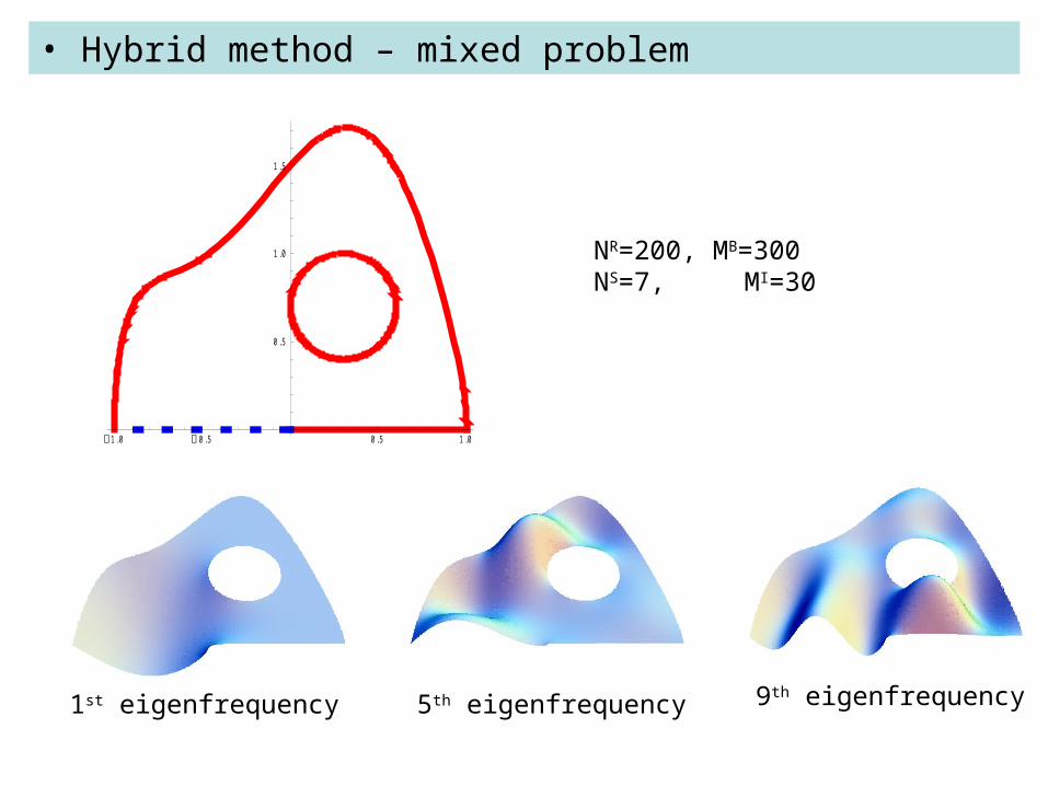
• Hybrid method – mixed problem
1.0 0.5 0.5 1.0
0.5
1.0
1.5
1st eigenfrequency 5th eigenfrequency 9th eigenfrequency
NR=200, MB=300NS=7, MI=30

Shape optimization problems

Given a quantity depending on some eigenvalues, we want to find a domain which optimizes
NQ ,...,1
Q
Direct setting
0
Inverse setting
• Shape optimization problems

Payne & Pölya & Weinberger (1956)
Ashbaugh & Benguria (1991) j
j2
1,0
2
1,1
1
2
There are some restrictions to the admissible sets of eigenvalues, eg.
n1n
3
• Inverse eigenvalue problems
Existence issue: The inverse problem may not have a solution.
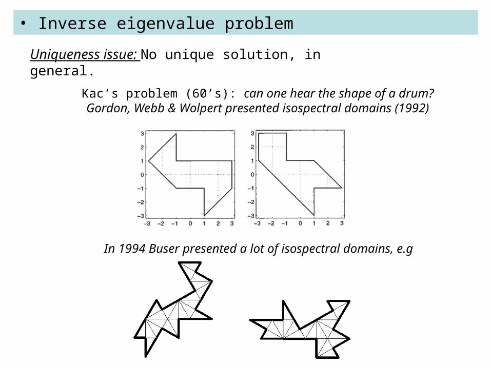
Kac’s problem (60’s): can one hear the shape of a drum?Gordon, Webb & Wolpert presented isospectral domains (1992)
In 1994 Buser presented a lot of isospectral domains, e.g
• Inverse eigenvalue problem
Uniqueness issue: No unique solution, in general.
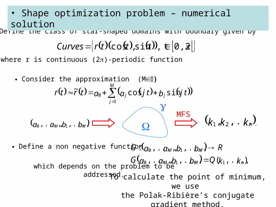
Define the class of star-shaped domains with boundary given by
0,2 t,sin,cos tttrCurveswhere r is continuous (2)-periodic function
M
jjj tjbtjaatrtr
10 sin cos~
Define a non negative function
which depends on the problem to be addressed.To calculate the point of minimum, we
use the Polak-Ribière’s conjugate gradient
method.
),...,(,...,,,...,
,...,,,...,:
110
10
kkQbbaaG
RbbaaG
nMM
MM
bbaa MM ,...,,,..., 10 kkk n,...,, 21
MFS
• Shape optimization problem – numerical solution
Consider the approximation (M)
Numerical resultsshape optimization problems

Which is the shape that maximizes and which is its maximum value?
In 2003 Levitin did a numerical study to find the optimal shape.
2
3
131,
k
kkkQ
1
3
We obtained 3.201999331
3 C
• Numerical results - shape optimization problems
.1
2
The ball maximizes Ashbaugh & Benguria (1991)
Optimal shape
L&Y = 3.202...

Is it possible to build a drum with an almost well defined pitch (fifth and the octave):
2 ;2
3
1
4
1
3
1
2 kk
kk
kk
1,999521,93272,07602k4 / k1
1,500931,52291,67641,5k3 / k1
1,500411,41731,56211,5k2 / k1
Our approach
Kane-Shoenauer 2
(1995)
Kane-Shoenauer 1
(1995)
“Harmonic
drum”
• Numerical results - shape optimization problem
Optimal shape
Can one hear the sound of Riemann Hypothesis?
A drum with the first 12 eigenfrequencies~ 12 first Im(zeros) of Zeta function
Is there a drum playing all the non trivial zeros of the Zeta function?
(modulo asymptotic behaviour)

shapes that minimize the eigenvalues 1 - the circle is the minimizer
2 - two circles minimize, … but the convex minimizer is unknown1973- Troesch - conjectured the stadium2002- Henrot&Oudet - reffuted - no circular parts
• Optimization problem (Dirichlet)
Numerical counterexample (Alves & A., 2005): Elliptical stadium
37.9875443 < 38.0021483 (stadium)
(3D)
• Numerical results - shape optimization problems

Other PDEs:Bilaplacian
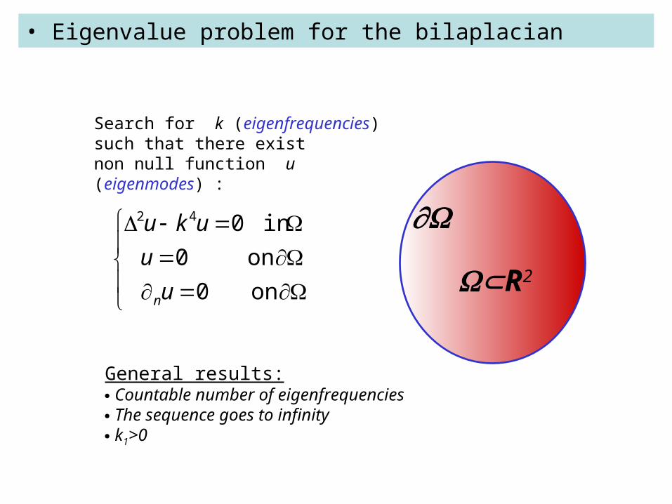
Search for k (eigenfrequencies) such that there exist non null function u (eigenmodes) :
on 0
on 0
in 0
42
u
u
uku
n
R2
• Eigenvalue problem for the bilaplacian
General results: Countable number of eigenfrequencies The sequence goes to infinity k1>0

~11
m
jjj
m
jjj yxnyxxuxu
y j
xHxiHi
x
2
01
028)(
• The MFS application to the bilaplacian problem
y j
Consider the approximation (m)
an admissible curve
Fundamental solution:
is analytic in satisfies the PDE
u~ u~

Given an open set 2, different points and kC,
are linearly independent on .
c
myy ,...,
1
)}(),...,(),(),...,({ 111
mm yxnyxnyxyxymy
• Theoretical results
If γ is the boundary of a domain which contains , the set
is dense in H3/2().
: :
yyxnyyxSpanxyx
Theorem (density result)
is not an eigenfrequency

DC
BAM Build the matrix M
di,j=xi-yj
,dA ji
,dnC jii
,dnB jij
,dnnD jiji
with the four blocks mm
• Eigenfrequency/eigenmode calculation
Eigenfrequency calculation
Define g(k)=|det(M(k))| and calculate the minima
Eigenmode calculation
Extra collocation point
12
22~
~
k
kk
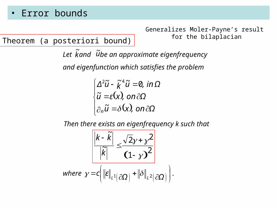
Let and be an approximate eigenfrequency
and eigenfunction which satisfies the problem
Then there exists an eigenfrequency k such that
Ω, on xu
Ω, on xεu
, in ΩukuΔ
n ~
~0~~~ 42
.21
ΩΩεc
LL
k~ u~
• Error bounds
Theorem (a posteriori bound)
where
Generalizes Moler-Payne’s result for the bilaplacian

m abs. error (k1) m abs. error (k2) m abs. error (k3)
20 4.2310-6 20 7.88 10-5 20 5.54 10-3
25 4.17 10-8 25 8.80 10-7 25 7.58 10-5
30 3.66 10-10 30 3.85 10-8 30 3.57 10-6
40 1.96 10-11 40 7.90 10-10 40 1.23 10-7
• Numerical results - bilaplacian

Plot of Log(g(k))Big rounding errors
• Numerical results – location of point sources
The proposed algorithm for the source points again presents more stable results

The eigenfunction associated to the first eigenvalue of the plate problem changes the sign “near” each corner
• Numerical simulations – equilateral triangle

3D plots and nodal domains for the 3rd,7th,10th and 11th resonance frequencies
• Numerical simulations – non trivial domains

Other PDEs:Elastodynamics (2D)

on 0
in 0)(
2
u
uu
R2
• Eigenvalue problem for elastodynamics
Fundamental solution: Kupradze’s tensor
MFS: Invertibility of the matrix

• Eigenvalue problem for elastodynamics - numerics
Test for the disk (6th eigenfrequency) with Poisson ratio =3/8
The choice of source points- same conclusions -
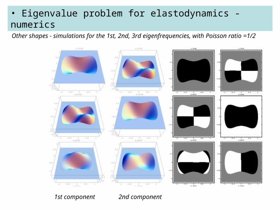
• Eigenvalue problem for elastodynamics - numerics
Other shapes - simulations for the 1st, 2nd, 3rd eigenfrequencies, with Poisson ratio =1/2
1st component 2nd component
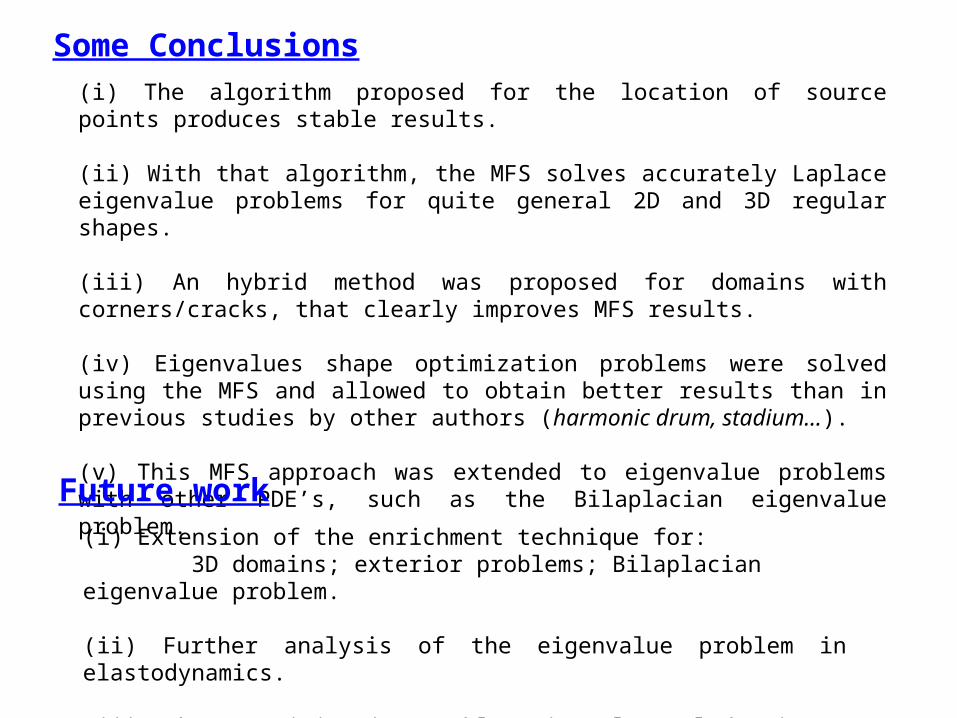
(i) The algorithm proposed for the location of source points produces stable results.
(ii) With that algorithm, the MFS solves accurately Laplace eigenvalue problems for quite general 2D and 3D regular shapes.
(iii) An hybrid method was proposed for domains with corners/cracks, that clearly improves MFS results.
(iv) Eigenvalues shape optimization problems were solved using the MFS and allowed to obtain better results than in previous studies by other authors (harmonic drum, stadium…).
(v) This MFS approach was extended to eigenvalue problems with other PDE’s, such as the Bilaplacian eigenvalue problem.
Some Conclusions
Future work(i) Extension of the enrichment technique for: 3D domains; exterior problems; Bilaplacian eigenvalue problem.
(ii) Further analysis of the eigenvalue problem in elastodynamics.
(iii) Shape optimization problems in polygonal domains


![ANTÓNIO LOBO ANTUNES: ORIGAMI ESPÁCIO-TEMPORAL“NIO LOBO ANTUNES: ORIGAMI ESPÁCIO-TEMPORAL [ANTÓNIO LOBO ANTUNES: SPATIOTEMPORAL ORIGAMI] by BRUNO GONÇALO NOGUEIRA SALES (Under](https://static.documents.pub/doc/80x56/5ae2d33b7f8b9ae74a8cf0db/antnio-lobo-antunes-origami-espcio-temporal-lobo-antunes-origami-espcio-temporal.jpg)


