Apriori • How to generate candidates? • Step 1: self-joining L k • Step 2: pruning • Example of Candidate-generation 1. L 3 = {abc, abd, acd, ace, bcd} 2. Self-joining L 3 ⨂ L 3 : abcd from abc and abd; acde from acd and ace 3. Pruning: acde is removed because ade is not in L 3 4. C 4 = {abcd}
Transcript
Apriori• How to generate candidates?
• Step 1: self-joining Lk
• Step 2: pruning
• Example of Candidate-generation
1. L3 = {abc, abd, acd, ace, bcd}
2. Self-joining L3 ⨂ L3: abcd from abc and abd; acde from acd and ace
3. Pruning: acde is removed because ade is not in L3
4. C4 = {abcd}
AprioriTid Items10 A, C, D20 B, C, E
30 A, B, C, E
40 B, E
Itemset sup{A} 2{B} 3
{C} 3
{D} 1
{E} 3
min_sup = 2C1
scan database for count of each
candidate
Itemset sup{A} 2{B} 3
{C} 3
{E} 3
Itemset{A, B}{A, C}
{A, E}
{B, C}
{B, E}
{C, E}
Itemset sup{A, B} 1{A, C} 2
{A, E} 1
{B, C} 2
{B, E} 3
{C, E} 2
Itemset sup{A, C} 2{B, C} 2
{B, E} 3
{C, E} 2
Itemset{B, C, E}
Itemset sup{B, C, E} 2
C2
scan database for count of
each candidatejoin and prune
scan database
C3/L3
join and prune
L1
compare candidate
support count with min_sup
L2
compare candidate
support count with min_sup
AprioriCk: Candidate itemset of size kLk: Frequent itemset of size k
L1 = {1-frequent items};for (k = 1; Lk !=∅; k++) do begin Ck+1 = candidates generated from Lk; for each transaction t in database do
increment the count of all candidates in Ck+1 that are contained in t
end Lk+1 = candidates in Ck+1 with min_supendreturn ⋃k Lk;
Apriori• How to count supports of each candidate?
• The total number of candidates can be huge
• One transaction may contain many candidates
• Support Counting Method:
• store candidate itemsets in a hash-tree
• leaf node of hash-tree contains a list of itemsets and counts
• interior node contains a hash table
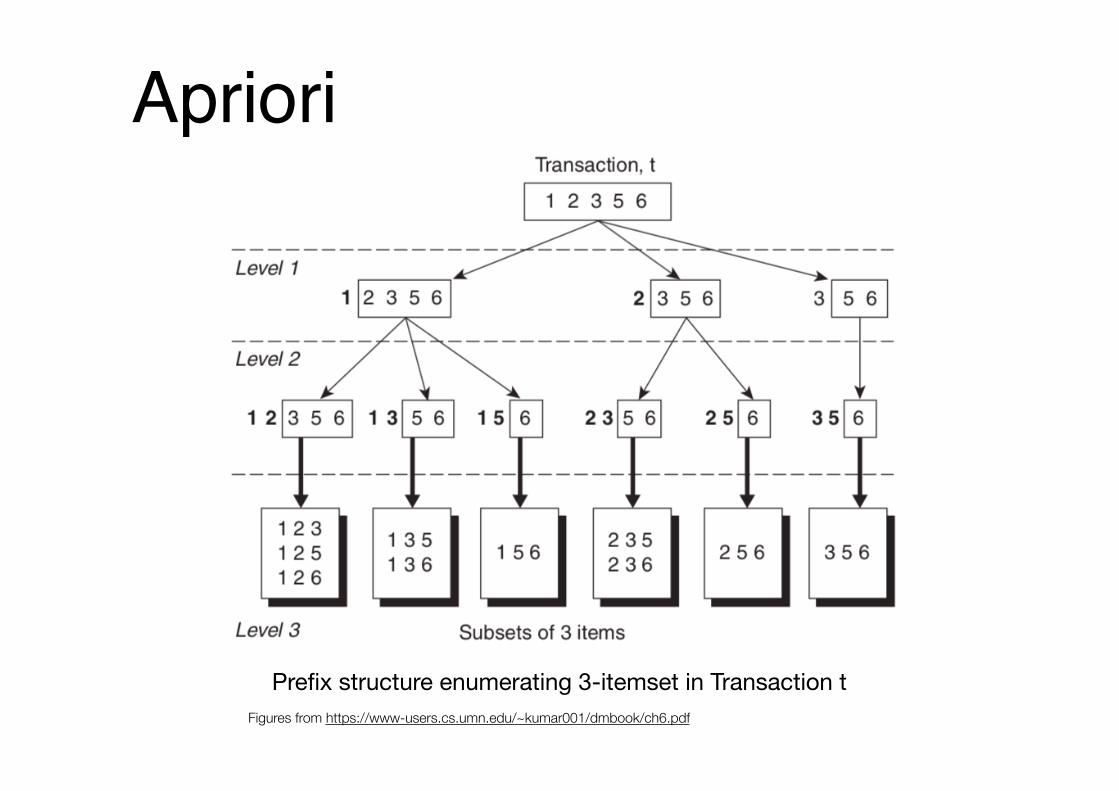
Apriori
Prefix structure enumerating 3-itemset in Transaction tFigures from https://www-users.cs.umn.edu/~kumar001/dmbook/ch6.pdf
Apriori
2 3 45 6 7
1 4 5 1 3 6
1 2 44 5 7 1 2 5
4 5 81 5 9
3 4 5 3 5 63 5 76 8 9
3 6 73 6 8
Transaction: 1 2 3 5 6
1 + 2 3 5 6
1 3 + 5 6
1 2 + 3 5 6
1,4,72,5,8
3,6,9
Hash functionh ( p ) = p mod 3
1 5 + 6
Improving the Efficiency of Apriori• Challenges:
• Multiple scans of transaction database
• Huge number of candidates
• Support counting for candidates
• Improving the Efficiency of Apriori
• Reduce passes of transaction database scans
• Shrink number of candidates
• Facilitate support counting of candidates
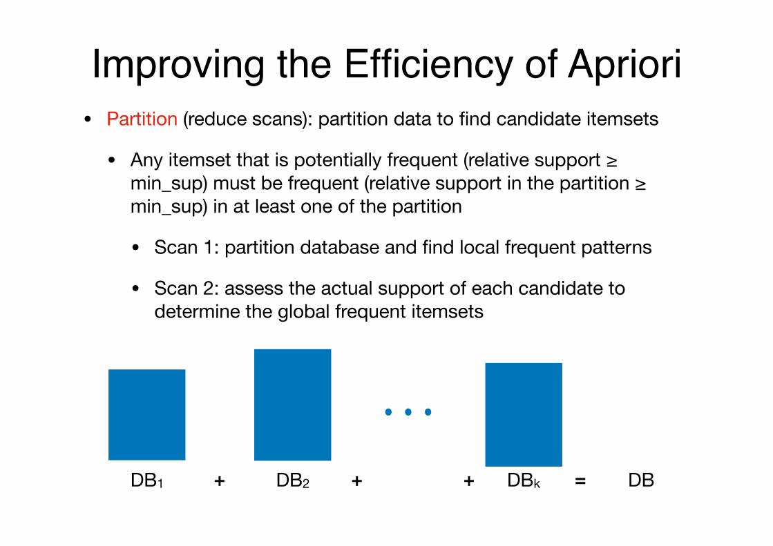
Improving the Efficiency of Apriori• Partition (reduce scans): partition data to find candidate itemsets
• Any itemset that is potentially frequent (relative support ≥ min_sup) must be frequent (relative support in the partition ≥ min_sup) in at least one of the partition
• Scan 1: partition database and find local frequent patterns
• Scan 2: assess the actual support of each candidate to determine the global frequent itemsets
DB1 DB2 DBk+ + + = DB
Improving the Efficiency of Apriori• Dynamic itemset counting (reduce
scans): adding candidate itemsets at different points during a scan
• new candidate itemsets can be added at any start point (rather than determined only before scan)
ABCD
ABC ABD ACD BCD
AB AC BC AD BD CD
A B C D
{}1-itemsets2-itemsets
…
1-itemsets2-items
3-items
Transactions
Apriori
DIC
• once both A and D are determined frequent, the counting of AD begins
• Once all length 2 subsets of BCD are determined frequent, the counting of BCD begins
Improving the Efficiency of Apriori• Hash-based Technique (shrink number of candidates): hashing
itemsets into corresponding buckets
• A k-itemset whose corresponding hashing bucket count is below min_sup cannot be frequent
Improving the Efficiency of Apriori• Sampling: mining on a subset of the given data
• Trade off some degree of accuracy against efficiency
• Select sample S of original database, mine frequent patterns within S (a lower support threshold) instead of the entire database —> the set of frequent itemsets local to S = LS
• Scan the rest of database once to compute the actual frequencies of each itemset in LS
• If LS actually contains all the frequent itemsets, stop; otherwise
• Scan database again for possible missing frequent itemsets
A Frequent-Pattern Growth Approach• Bottlenecks of Apriori
• Breadth-first (i.e., level-wise) search
• Candidate generation and test, often generates a huge number of candidates
• FP-Growth
• Depth-first search
• Avoid explicit candidate generation
• Grow long patterns from short ones using local frequent items
• “abc” is a frequent pattern
• Get all transactions having “abc,” i.e., project database D on abc: D | abc
• “d” is a local frequent item in D | abc —> abcd is a frequent pattern
A Frequent-Pattern Growth Approach
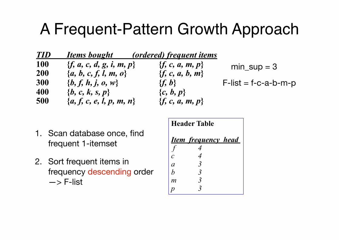
1. Scan database once, find frequent 1-itemset
2. Sort frequent items in frequency descending order —> F-list
TID Items bought (ordered) frequent items100 {f, a, c, d, g, i, m, p} {f, c, a, m, p}200 {a, b, c, f, l, m, o} {f, c, a, b, m}300 {b, f, h, j, o, w} {f, b}400 {b, c, k, s, p} {c, b, p}500 {a, f, c, e, l, p, m, n} {f, c, a, m, p}
min_sup = 3
F-list = f-c-a-b-m-p
Header Table
Item frequency head f 4c 4a 3b 3m 3p 3
A Frequent-Pattern Growth Approach
1. Scan database once, find frequent 1-itemset
2. Sort frequent items in frequency descending order —> F-list
3. Scan database again, construct FP-tree
4. Mine FP-tree
TID Items bought (ordered) frequent items100 {f, a, c, d, g, i, m, p} {f, c, a, m, p}200 {a, b, c, f, l, m, o} {f, c, a, b, m}300 {b, f, h, j, o, w} {f, b}400 {b, c, k, s, p} {c, b, p}500 {a, f, c, e, l, p, m, n} {f, c, a, m, p}
min_sup = 3
{}
f:4 c:1
b:1
p:1
b:1c:3
a:3
b:1m:2
p:2 m:1
Header Table
Item frequency head f 4c 4a 3b 3m 3p 3
F-list = f-c-a-b-m-p
How to Construct FP-tree?
{}
f:4 c:1
b:1
p:1
b:1c:3
a:3
b:1m:2
p:2 m:1
Header Table
Item frequency head f 4c 4a 3b 3m 3p 3
FP-tree: a compressed representation of database.It retains the itemset association information.
1. Start from each frequent length-1 pattern (suffix pattern, usually the last item in F-list) to construct its conditional pattern base (prefix paths co-occurring with the suffix)
How to Mine FP-tree?1. Start from each frequent length-1 pattern (suffix pattern, usually
the last item in F-list) to construct its conditional pattern base2. Construct the conditional FP-tree based on the conditional
pattern base
{}
f:3
c:3
a:3m-conditional FP-tree
m-conditional pattern base:fca:2, fcab:1
{}
f:4 c:1
b:1
p:1
b:1c:3
a:3
b:1m:2
p:2 m:1
Header TableItem frequency head f 4c 4a 3b 3m 3p 3
How to Mine FP-tree?1. Start from each frequent length-1 pattern (suffix pattern, usually
the last item in F-list) to construct its conditional pattern base2. Construct the conditional FP-tree based on the conditional
pattern base3. Mining recursively on each conditional FP-tree until the resulting
FP-tree is empty, or it contains only a single path — which will generate frequent patterns out of all combinations of its sub-paths
{}
f:3
c:3
a:3m-conditional FP-tree
m-conditional pattern base:fca:2, fcab:1
{}
f:3
c:3am-conditional FP-tree
fc: 3
{}
f:3cm-conditional FP-tree
f: 3
{}
f:3cam-conditional FP-tree
f: 3
All frequent patterns
relating to m: m, fm, cm, am, fcm, fam, cam,
fcam
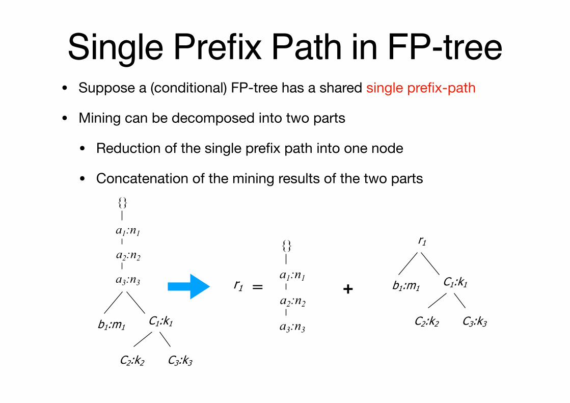
Single Prefix Path in FP-tree• Suppose a (conditional) FP-tree has a shared single prefix-path
• Mining can be decomposed into two parts
• Reduction of the single prefix path into one node
• Concatenation of the mining results of the two parts
a2:n2
a3:n3
a1:n1
{}
b1:m1 C1:k1
C2:k2 C3:k3
a2:n2
a3:n3
a1:n1
{}
r1 = b1:m1 C1:k1
C2:k2 C3:k3
r1
+
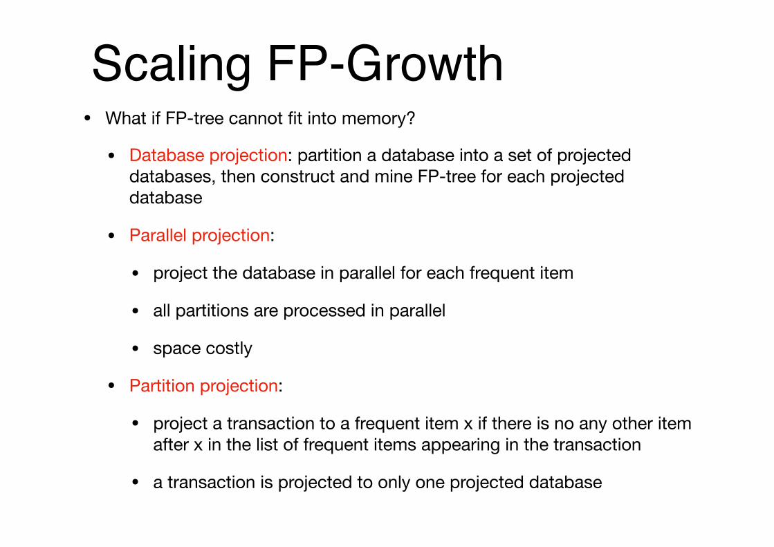
Scaling FP-Growth• What if FP-tree cannot fit into memory?
• Database projection: partition a database into a set of projected databases, then construct and mine FP-tree for each projected database
• Parallel projection:
• project the database in parallel for each frequent item
• all partitions are processed in parallel
• space costly
• Partition projection:
• project a transaction to a frequent item x if there is no any other item after x in the list of frequent items appearing in the transaction
• a transaction is projected to only one projected database
Benefits of FP-tree• Completeness
• Preserve complete information for frequent pattern mining
• Never break a long pattern of any transaction
• Compactness
• Reduce irrelevant info — infrequent items are gone
• Items in frequency descending order: occurs more frequently, the more likely to be shared
• Never be larger than the original database (not including node-links and the count fields)
Benefits of FP-Growth• Divide-and-conquer:
• Decompose both the mining task and database according to the frequent patterns obtained so far
• Lead to focused search of smaller databases
• Other factors:
• No candidate generation, no candidate test
• Compressed database: FP-tree
• No repeated scan of the entire database
• Basic operations: count local frequent items and build sub FP-tree, no pattern search and matching
Performance of FP-Growth in Large Datasets
0
10
20
30
40
50
60
70
80
90
100
0 0.5 1 1.5 2 2.5 3Support threshold(%)
Run
time(
sec.
)D1 FP-grow th runtime
D1 Apriori runtime
FP-Growth vs. Apriori
ECLAT: Frequent Pattern Mining with Vertical Data Format• Vertical data format: itemset — transID_set
• transID_set: a set of transaction IDs containing the itemset
• Derive frequent patterns based on the intersections of transID_set
ECLAT: Frequent Pattern Mining with Vertical Data Format• Vertical data format: itemset — transID_set
• transID_set: a set of transaction IDs containing the itemset
• Derive frequent patterns based on the intersections of transID_set
• Use diffset to reduce the cost of storing long transID_set