Computational Study of Three Numerical Methods for Some Linear and Non-Linear Advection-Diffusion-Reaction Problems A.R. Appadu 1 , J.M.-S Lubuma 2 and N. Mphephu 3 1,2,3 Department of Mathematics and Applied Mathematics, University of Pretoria, Pretoria, 0002, South Africa. Corresponding author: 1 Email: [email protected] or [email protected], 2 Email: [email protected], 3 Email: [email protected]. Abstract In this paper, we use three existing schemes namely, Upwind Forward Euler, Non-Standard Finite Dif- ference (NSFD) and Unconditionally Positive Finite Difference (UPFD) schemes to solve two numerical experiments described by a linear and a non-linear advection-diffusion-reaction equation with constant coefficients. These equations model exponential travelling waves and biofilm growth on a medical im- plant respectively. We study the exact and numerical dissipative and dispersive properties of the three schemes for both problems. Moreover, L 1 error, dispersion and dissipation errors, at some values of temporal and spatial step sizes have been computed for the three schemes for both problems. Keywords: advection-diffusion-reaction, stability, dispersion, dissipation, finite difference. 1 Introduction The advection-diffusion-reaction partial differential equation provides a very useful and important math- ematical model in a wide range of applications in natural sciences and engineering [10]. These applica- tions include the transport of air, adsorption of pollutants in soil, diffusion of neutrons, food processing, modelling of biological systems, modelling of semiconductors, oil reservoir flow transport and reaction of chemical species etc. In hydrology, equations of this type govern the fate and transport of reactive pollutants and biofilm-forming microbes in porous media. These equations are often used to predict and control the extent of contamination in ground water systems [7]. In many of these applications, the unknown variables in the governing partial differential equation represent physical quantities that cannot take negative values such as pollutants, population, concentration of chemical compounds [6]. The application of advection-diffusion-reaction (ADR) equation is classified into three processes [9]. The first process is called convection and is due to movement of materials from one region to another. The second process is called diffusion and is due to movement of materials from a region of high con- centration to a region of lower concentration. The last process is called reaction and is due to decay, adsorption and reaction of substances with other components. Qualitatively all the three processes form the ADR model that describe how the disturbed quantity being studied in the medium changes under the influence of these processes [9]. In many applications, the governing partial differential equation is non-linear elliptic and the analytical solution is not easy to find [10]. The difficulties in obtaining analytical solution lead many researchers and engineers to resort to numerical methods for approximating the solution to the problem. These numerical methods have been active for about fifty years now and the development of new techniques still attracts more attention [9]. However, there are also some challenges when applying these numer- ical methods to approximate the solution to problems that are non-linear. One of the challenges is numerical instabilities [10]. For the ADR model dominated with diffusion, the standard finite difference methods (SFDM) and finite element method (FEM) produce satisfactory results while for problems dominated by convection, numerical instabilities like oscillations and numerical dispersion appear in the solution approximated by these methods [9]. These numerical instabilities can be overcomed for instance 1
Transcript
Computational Study of Three Numerical Methods for Some Linear and Non-LinearAdvection-Diffusion-Reaction Problems
A.R. Appadu1, J.M.-S Lubuma2 and N. Mphephu3
1,2,3 Department of Mathematics and Applied Mathematics, University of Pretoria, Pretoria, 0002,South Africa.
AbstractIn this paper, we use three existing schemes namely, Upwind Forward Euler, Non-Standard Finite Dif-ference (NSFD) and Unconditionally Positive Finite Difference (UPFD) schemes to solve two numericalexperiments described by a linear and a non-linear advection-diffusion-reaction equation with constantcoefficients. These equations model exponential travelling waves and biofilm growth on a medical im-plant respectively. We study the exact and numerical dissipative and dispersive properties of the threeschemes for both problems. Moreover, L1 error, dispersion and dissipation errors, at some values oftemporal and spatial step sizes have been computed for the three schemes for both problems.
The advection-diffusion-reaction partial differential equation provides a very useful and important math-ematical model in a wide range of applications in natural sciences and engineering [10]. These applica-tions include the transport of air, adsorption of pollutants in soil, diffusion of neutrons, food processing,modelling of biological systems, modelling of semiconductors, oil reservoir flow transport and reactionof chemical species etc. In hydrology, equations of this type govern the fate and transport of reactivepollutants and biofilm-forming microbes in porous media. These equations are often used to predictand control the extent of contamination in ground water systems [7]. In many of these applications,the unknown variables in the governing partial differential equation represent physical quantities thatcannot take negative values such as pollutants, population, concentration of chemical compounds [6].The application of advection-diffusion-reaction (ADR) equation is classified into three processes [9].The first process is called convection and is due to movement of materials from one region to another.The second process is called diffusion and is due to movement of materials from a region of high con-centration to a region of lower concentration. The last process is called reaction and is due to decay,adsorption and reaction of substances with other components. Qualitatively all the three processes formthe ADR model that describe how the disturbed quantity being studied in the medium changes underthe influence of these processes [9].
In many applications, the governing partial differential equation is non-linear elliptic and the analyticalsolution is not easy to find [10]. The difficulties in obtaining analytical solution lead many researchersand engineers to resort to numerical methods for approximating the solution to the problem. Thesenumerical methods have been active for about fifty years now and the development of new techniquesstill attracts more attention [9]. However, there are also some challenges when applying these numer-ical methods to approximate the solution to problems that are non-linear. One of the challenges isnumerical instabilities [10]. For the ADR model dominated with diffusion, the standard finite differencemethods (SFDM) and finite element method (FEM) produce satisfactory results while for problemsdominated by convection, numerical instabilities like oscillations and numerical dispersion appear in thesolution approximated by these methods [9]. These numerical instabilities can be overcomed for instance
1
by applying the Non-Standard Finite Difference methods (NSFD). These methods are now playing animportant role in the design of reliable numerical schemes in several areas of science and engineering [12].
In this paper, we focus on the application of standard and Non-Standard Finite Difference methodsto solve the one dimensional advection-diffusion-reaction equation. This equation takes the form
∂u
∂t+
∂
∂x(au) =
∂
∂x
(D∂u
∂x
)+ f(u),
where u(x, t) is the unknown quantity being investigated, a(x, t) is the velocity of the medium (alsocalled convective velocity), D(x, t) is the diffusion coefficient and f(u) is the reaction source. Thenovelty in this work in regard to work in [6] is that the stability of the schemes have been obtainedand hence it allows a more effective way of comparing the performance of the three schemes. Also,dissipation and dispersion properties of the schemes are studied.The paper is organised as follows. In sections 2 and 3, we describe the numerical experiments consideredand how the quantification of errors is implemented. In section 4, we study the stability, consistency,spectral analysis of three schemes when used to discretise ut+ux−uxx = −u and present the numericalresults in section 5. Sections 6 and 7 discuss the stability, consistency, spectral analysis of the threemethods when applied to ut − (Dux)x = ru(1 − u) and numerical results are presented. Section 8highlights the salient features of the paper.
2 Numerical Experiments
We consider two problems. First, we consider the advection-diffusion-reaction equation for modellingthe exponential travelling waves [6]. This equation is given by
∂u
∂t+
∂u
∂x− ∂2u
∂x2= −u, (x, t) ∈ [0, 10]× [0, 0.85], (1)
subject to the following initial condition and boundary conditions :
u(x, 0) = e−x, 0 ≤ x ≤ 10,
u(0, t) = et, 0 ≤ t ≤ 0.85, and
ux(10, t) = −u(10, t), 0 ≤ t ≤ 0.85.
Eq.(1) together with its initial and boundary conditions has the exact solution given by
u(x, t) = e(t−x). (2)
The most realistic applications involving equation Eq.(1) are for complex systems and as a result therewill be grid spacing limitation on the numerical method. Thus, if the grid spacing is not fine enough, thenumerical scheme will not compute stable solutions. Different methods have been proposed increasinglocal grid refinement only in those regions where the solution is changing rapidly [15].
Secondly, we consider the advection-diffusion-reaction equation for modelling biofilm growth on a med-ical implant [6]. This equation is given by
∂u
∂t− ∂
∂x
(D∂u
∂x
)= ru (1− u) , (x, t) ∈ [0, 1]× [0, 13], (3)
2
with initial and boundary conditions given by
u(x, 0) =
{0.7 e−σ(x−x0)2 , |x− x0| ≤ 0.060, otherwise
and
u(0, t) = 0 , 0 ≤ t ≤ 13,
u(1, t) = 0 , 0 ≤ t ≤ 13.
Eq.(3) together with the initial and boundary conditions have its exact solution described by a travellingwave like solution [13] which is given by
u(x, t) =1[
1 +
(1−√
u(x,0)√u(x,0) exp( 1
6D
√6Drx)
)exp
(−5
6rt+16D
√6Drx
)]2 . (4)
We solve problem 2 described by Eq.(3) using the same parameters as in [6], namely D = 0.0002,x0 = 0.5, r = 0.05 and σ = 80.
3 Quantification of Errors
To quantify the errors from numerical results into dispersion and dissipation errors, we follow the workof Takacs [18]. We let um represent the analytical solution and vm represent the numerical solution, atgrid point, m. Then, the absolute error is given by
E = |um − vm|.
The Total Mean Square Error is calculated as
ETMS =1
N
N∑m=1
(um − vm
)2, or
ETMS =1
N
N∑m=1
u2m − 2
N
N∑m=1
umvm +1
N
N∑m=1
v2m,
where N is the number of grid points.
The sample variances for the analytical and numerical solutions are respectively given by
δ2(u) =1
N
N∑m=1
(um − u
)2, and
δ2(v) =1
N
N∑m=1
(vm − v
)2, where u and v are the means of u and v respectively.
h2 , k and h are the temporal and spatial step sizes respectively.
Stability
To obtain the region of stability of the finite difference scheme, we use the Fourier series analysis. Theamplification factor is given by
ξ = 1− k − (λ+ 2β)(1− cosω)− Iλ sinω, (9)
where ω is the phase angle, ω = θh where θ is the wavenumber and h is the spatial step size.
The scheme is stable whenever the Von-Neumann condition, |ξ| ≤ 1 is satisfied. The modulus ofamplification factor is given by
|ξ| =√
[ℜ(ξ)]2 + [ℑ(ξ)]2,
where ℜ(ξ) and ℑ(ξ) are the real and imaginary parts of ξ respectively. The modulus of the amplificationfactor of the scheme given by Eq. (8) is obtained as
|ξ| =
√[1− k −
(k
h+
2k
h2
)[1− cos(ω)]
]2+
[k sin(ω)
h
]2, (10)
with −π ≤ ω ≤ π.
We choose h = 0.1 as in the numerical experiment we have worked with h = 0.1. We thus get
|ξ|2 = [1− k − 210k(1− cos(ω))]2 + (10 k sin(ω))2. (11)
We then use maple software to solve for |ξ|2 ≤ 1 for ω ∈ [−π, π] and we obtain the region of stabilityas 0 < k ≤ 0.00475.
5
Consistency
To study the consistency of the Upwind Forward Euler finite difference scheme, we need to first obtainthe Taylor expansion of the terms in Eq.(8) about the point (m,n). We assume that u is continuousand that the derivatives of u are bounded. The Taylor series expansion of un+1
m , unm+1 and unm−1 aboutthe point (m,n) are respectively given by
un+1m = unm + k
∂u
∂t+
k2
2!
∂2u
∂t2+
k3
3!
∂3u
∂t3+ · · · (12)
unm+1 = unm + h∂u
∂x+
h2
2!
∂2u
∂x2+
h3
3!
∂3u
∂x3+ · · · (13)
unm−1 = unm − h∂u
∂x+
h2
2!
∂2u
∂x2− h3
3!
∂3u
∂x3+ · · · (14)
Substituting Eqs.(12)-(14) in Eq.(8) and simplifying, we obtain
∂u
∂t+
∂u
∂x− ∂2u
∂x2= −u− k
2
∂2u
∂t2− k2
6
∂3u
∂t3+
h
2
∂2u
∂x2− h2
6
∂3u
∂x3+ · · · (15)
As k → 0 and h → 0 , Eq.(15) reduces to Eq.(1) and therefore, the Upwind Forward Euler finitedifference scheme is consistent.
Spectral Analysis
We study the dissipative and dispersive behaviour of the Upwind Forward Euler finite difference schemewhen h = 0.1 at some different values of k. The values of k were chosen such that they are less than orequal to the upper bound of the region of stability.
We let the elementary solution to Eq.(1) be [14]
u(x, t) = eαt eIθx. (16)
where α is the dispersion relation and θ is the wave number.
Using Eq.(16) and Eq.(1) and solving for the dispersion relation, α we obtain
α = −1− θ2 − Iθ. (17)
As a result of Eq.(17), the elementary solution is now expressed as
u(x, t) = e(−1−θ2)t e−Iθt eIθx. (18)
The term e(−1−θ2)t e−Iθt shows that the amplitude of the solution is decaying exponentially and hencethe exact amplification factor is given by
ξexact =e(−1−θ2)(n+1)k e−Iθ(n+1)k
e(−1−θ2)nk e−Iθnk,
= e(−1−θ2)k e−Iθk. (19)
Equivalently, the exact amplification factor can be expressed as
ξexact = (cos(θk)− I sin(θk)) e−(1+θ2)k. (20)
6
The relative phase error, is given by
RPE =arg(ξnum)
arg(ξexact), (21)
=arg(ξnum)
tan−1(− tan(θk)),
= − 1
kθarg(ξnum),
= − 1
kθtan−1
(ℜ(ξnum)ℑ(ξnum)
).
where ξnum is the numerical amplification factor obtained from the Fourier series analysis. Thus therelative phase error for the Upwind Forward Euler scheme is given by
RPE =1
kθtan−1
(λ sinω
1− k − (λ+ β)(1− cosω)
). (22)
We next obtain plots of the variation of the modulus of exact amplification factor (exact AFM) andmodulus of the numerical amplification factor (numerical AFM), both versus phase angle at h = 0.1and at some different values of k in Fig. (1).
Figure 1: Plots of the exact AFM and AFM for Upwind Forward Euler scheme for Eq.(1), at somevalues of k with h = 0.1.
8
0 0.5 1 1.5 2 2.5 3 3.50
0.2
0.4
0.6
0.8
1
1.2
1.4
ω
RP
E
k = 0.001k = 0.85/527k = 0.002
(a)
0 0.5 1 1.5 2 2.5 30
1
2
3
4
5
6
7
8
9
10
k = 0.85/180 → ← k = 0.85/212
ω
RP
E
(b)
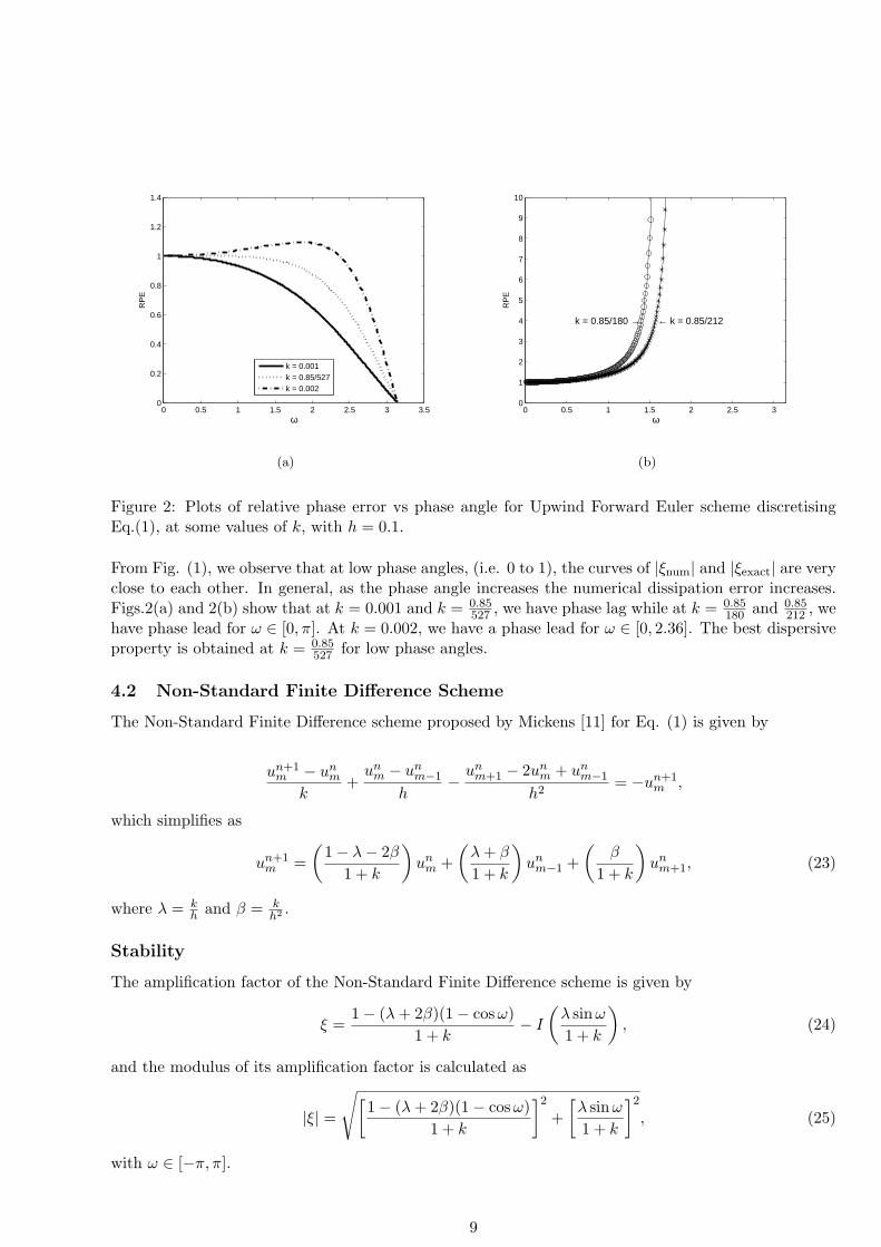
Figure 2: Plots of relative phase error vs phase angle for Upwind Forward Euler scheme discretisingEq.(1), at some values of k, with h = 0.1.
From Fig. (1), we observe that at low phase angles, (i.e. 0 to 1), the curves of |ξnum| and |ξexact| are veryclose to each other. In general, as the phase angle increases the numerical dissipation error increases.Figs.2(a) and 2(b) show that at k = 0.001 and k = 0.85
527 , we have phase lag while at k = 0.85180 and 0.85
212 , wehave phase lead for ω ∈ [0, π]. At k = 0.002, we have a phase lead for ω ∈ [0, 2.36]. The best dispersiveproperty is obtained at k = 0.85
527 for low phase angles.
4.2 Non-Standard Finite Difference Scheme
The Non-Standard Finite Difference scheme proposed by Mickens [11] for Eq. (1) is given by
un+1m − unm
k+
unm − unm−1
h−
unm+1 − 2unm + unm−1
h2= −un+1
m ,
which simplifies as
un+1m =
(1− λ− 2β
1 + k
)unm +
(λ+ β
1 + k
)unm−1 +
(β
1 + k
)unm+1, (23)
where λ = kh and β = k
h2 .
Stability
The amplification factor of the Non-Standard Finite Difference scheme is given by
ξ =1− (λ+ 2β)(1− cosω)
1 + k− I
(λ sinω
1 + k
), (24)
and the modulus of its amplification factor is calculated as
|ξ| =
√[1− (λ+ 2β)(1− cosω)
1 + k
]2+
[λ sinω
1 + k
]2, (25)
with ω ∈ [−π, π].
9
On plugging h = 0.1, we get
|ξ|2 = (1− 210 k (1− cos(ω))2 + (10 k sin(ω))2
(1 + k)2. (26)
Solving |ξ|2 ≤ 1 for ω ∈ [−π, π] gives the region of stability as 0 < k ≤ 0.00477.
Consistency
To study the consistency of the Non-Standard Finite Difference scheme, we substitute Eqs.(12)-(14) inEq. (23). Substituting these equations and simplifying, we obtain
∂u
∂t+
∂u
∂x− ∂2u
∂x2= −u− k
∂u
∂t+
(k2
2− k
2
)∂2u
∂t2+
(k3
6− k2
6
)∂3u
∂t3+
h
2
∂2u
∂x2
− h2
2
∂3u
∂x3+ · · · (27)
As k → 0 and h → 0, Eq.(27) reduces to Eq.(1), hence the scheme is consistent.
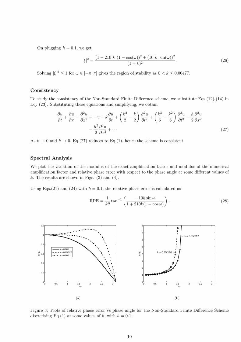
Spectral Analysis
We plot the variation of the modulus of the exact amplification factor and modulus of the numericalamplification factor and relative phase error with respect to the phase angle at some different values ofk. The results are shown in Figs. (3) and (4).
Using Eqs.(21) and (24) with h = 0.1, the relative phase error is calculated as
RPE =1
kθtan−1
(−10k sinω
1 + 210k(1− cosω)
). (28)
0 0.5 1 1.5 2 2.5 30
0.2
0.4
0.6
0.8
1
1.2
ω
RP
E
k = 0.001k = 0.85/527k = 0.002
(a)
0 0.5 1 1.5 2 2.5 30
1
2
3
4
5
6
7
8
k = 0.85/180 →
← k = 0.85/212
ω
RP
E
(b)
Figure 3: Plots of relative phase error vs phase angle for the Non-Standard Finite Difference Schemediscretising Eq.(1) at some values of k, with h = 0.1.
Figure 4: Plot of the exact AFM and AFM of the Non-Standard Finite Difference scheme for Eq. (1),at some values of k, with h = 0.1.
Based on Figs.(2) and (3), we observed that the dispersive behaviours of Non-Standard Finite Differencescheme is better than that of the Upwind Forward Euler scheme.
When discretised by the Unconditionally Positive Finite Difference Scheme [6], Eq.(1) gives
un+1m − unm
k+
un+1m − unm−1
h−
unm+1 − 2un+1m + unm−1
h2= −un+1
m ,
which simplifies as
un+1m =
unm + (λ+ β)unm−1 + βunm+1
1 + k + λ+ 2β, (29)
11
where λ = kh and β = k
h2 .
Stability
The amplification factor of the UPFD scheme is given by
ξ =1 + (λ+ 2β) cosω
1 + k + λ+ 2β− I
[λ sinω
1 + k + λ+ 2β
]. (30)
The scheme is positive definite for all k, h > 0. Hence, the scheme is unconditionally stable for allh, k > 0.
Consistency
To obtain the truncation errors for the Unconditionally Positive Finite Difference method, we substi-tute Eqs.(12)-(14) in the finite difference scheme given by Eq.(29). Substituting these equations andsimplifying, we obtain
∂u
∂t+
∂u
∂x− ∂2u
∂x2= −u−
(k +
k
h+
2k
h2
)∂u
∂t−(k
2+
k2
2+
k2
2h+
k2
h2
)∂2u
∂t2
−(k2
6+
k3
6+
k3
6h+
k3
3h2
)∂3u
∂t3+
h
2
∂2u
∂x2− h2
6
∂3u
∂x3+ · · · (31)
For the scheme to be consistent, we require k = h3 which gives
∂u
∂t+
∂u
∂x− ∂2u
∂x2= −u−
(h3 + h2 + 2h
)∂u
∂t− h3
2
(1 + h2 + 2h+ h3
)∂2u
∂t2
− h6
6
(1 + h2 + 2h+ h3
)∂3u
∂t3+
h
2
∂2u
∂x2− h2
6
∂3u
∂x3+ · · · (32)
When h → 0 we can see that Eq.(32) reduces to Eq.(1), hence the Unconditionally Positive FiniteDifference Scheme is consistent when k = h3.
Spectral Analysis
Using Eqs. (17) and (30) with h = 0.1, the relative phase error is given by
RPE =1
kθtan−1
(−10k sinω
1 + 210k cosω
). (33)
12
0 0.5 1 1.5 2 2.5 30
0.2
0.4
0.6
0.8
1
ω
|ξ|
ExactNumerical
Figure 5: Plot of the exact AFM and AFM of the Unconditionally Positive Finite Difference scheme forEq.(1) with k = 0.001 and h = 0.1.
0 0.5 1 1.5 2 2.5 30
0.2
0.4
0.6
0.8
1
1.2
ω
RP
E
Figure 6: Plot of relative phase error vs phase angle for Unconditionally Positive Finite DifferenceScheme discretising Eq.(1) with k = 0.001 and h = 0.1.
The plots of the modulus of amplification factor and relative phase error are shown in Figs. (5) and(6). We note that the relative phase error for the scheme is not one when ω = 0. This could be due tothe presence of extra truncation error terms resulting from the approximation of first and second order
derivative terms∂u
∂x,∂2u
∂x2at different time levels. Also, we observe that the scheme is less dissipative
than the partial differential equation as the phase angle increases.
5 Numerical Results for Experiment 1
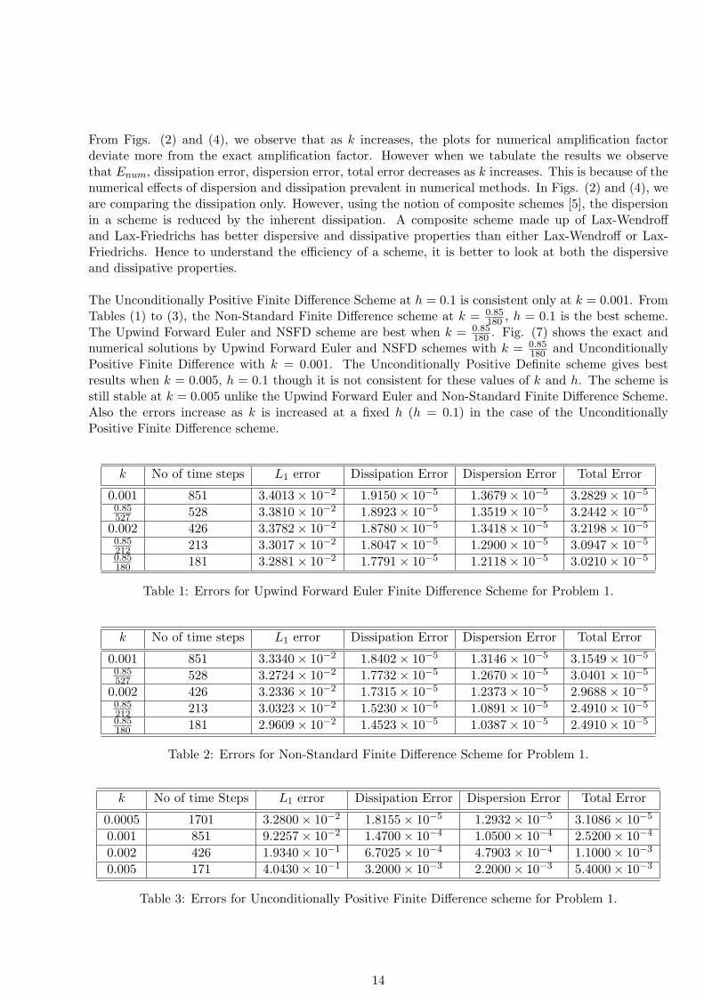
We tabulate the error rate with respect to L1 norm, dissipation, dispersion, and total errors in Tables(1) to (3) for the three numerical schemes.We observe that for the Upwind Forward Euler and NSFD schemes, the errors are dependent on thetemporal step size when h is chosen as 0.1. The errors decrease as k is increased, at a fixed h whichis 0.1. Also, the dissipation error is slightly greater than the dispersion error for the five values of kchosen for both schemes.
13
From Figs. (2) and (4), we observe that as k increases, the plots for numerical amplification factordeviate more from the exact amplification factor. However when we tabulate the results we observethat Enum, dissipation error, dispersion error, total error decreases as k increases. This is because of thenumerical effects of dispersion and dissipation prevalent in numerical methods. In Figs. (2) and (4), weare comparing the dissipation only. However, using the notion of composite schemes [5], the dispersionin a scheme is reduced by the inherent dissipation. A composite scheme made up of Lax-Wendroffand Lax-Friedrichs has better dispersive and dissipative properties than either Lax-Wendroff or Lax-Friedrichs. Hence to understand the efficiency of a scheme, it is better to look at both the dispersiveand dissipative properties.
The Unconditionally Positive Finite Difference Scheme at h = 0.1 is consistent only at k = 0.001. FromTables (1) to (3), the Non-Standard Finite Difference scheme at k = 0.85
180 , h = 0.1 is the best scheme.The Upwind Forward Euler and NSFD scheme are best when k = 0.85
180 . Fig. (7) shows the exact andnumerical solutions by Upwind Forward Euler and NSFD schemes with k = 0.85
180 and UnconditionallyPositive Finite Difference with k = 0.001. The Unconditionally Positive Definite scheme gives bestresults when k = 0.005, h = 0.1 though it is not consistent for these values of k and h. The scheme isstill stable at k = 0.005 unlike the Upwind Forward Euler and Non-Standard Finite Difference Scheme.Also the errors increase as k is increased at a fixed h (h = 0.1) in the case of the UnconditionallyPositive Finite Difference scheme.
k No of time steps L1 error Dissipation Error Dispersion Error Total Error
Figure 7: Plots of numerical solution from Upwind Forward Euler, Non-Standard Finite Difference andUnconditionally Positive Finite Difference schemes at time, T = 0.85.
0 2 4 6 8 100
0.005
0.01
0.015
0.02
0.025
0.03
0.035
0.04
x
Abs
olut
e er
ror
UpwindNSFDUPFD
(a) k = 0.001
0 2 4 6 8 100
0.005
0.01
0.015
0.02
0.025
0.03
0.035
0.04
x
Abs
olut
e er
ror
UpwindNSFDUPFD
(b) k = 0.85180
Figure 8: Plots of absolute errors from Upwind Forward Euler, Non-Standard Finite Difference andUnconditionally Positive Finite Difference schemes at time, T = 0.85.
15
(a) Upwind Forward Euler scheme with k = 0.85180
. (b) NSFD scheme with k = 0.85180
.
(c) UPFD scheme with k = 0.001.
Figure 9: Numerical solutions using Upwind Forward Euler, NSFD and UPFD schemes plotted vst ∈ [0, 0.85] vs x ∈ [0, 10].
6 Numerical Solution of ut − (Dux)x = ru(1− u)
In this section, we use the three methods discussed in section 5 in order to solve ut−(Dux)x = ru(1−u),subject to specified initial and boundary conditions.
The Fourier series analysis can only be applied directly to linear problems with constant coefficients.Since our problem is non-linear, the method will have a drawback. To overcome this drawback, welinearise the problem and freeze the coefficients[8]. The Fourier series analysis can then be applied todetermine the region of stability thereafter.
Taha and Ablowitz [16] have obtained the stability of a scheme proposed by Zabusky and Kruskal [17]for the KdV equation using the method of freezing coefficients. The scheme derived by Zabusky andKruskal for the KdV equation, ut + 6 u ux + uxxx = 0 is
un+1m = un−1
m − 2k
h(unm+1 + unm + unm−1) (u
nm+1 − unm−1)−
k
h3(unm+2 − 2unm+1 + 2unm−1 − unm−2).
Using the method of freezing coefficients and Fourier analysis, they write uux as umax ux and substitutethe ansatz unm = ξn exp(Imω) where ω is the phase angle.The amplification polynomial is given by
ξ = ξ−1 − 2k
humax(2I sin(ω))−
k
h3
(exp(2Iω)− 2 exp(Iω) + 2 exp(−Iω)− exp(−2Iω)
),
and the region of stability is obtained as
k
h≤ 2
3√3(2 umax − 1
h2 ).
We use the same approach used by Taha and Ablowitz to obtain the stability of schemes discretisingut − (Dux)x = ru(1− u).
Using Eq.(34), we have
un+1m = unm +
Dk
h2(unm+1 − 2unm + unm−1
)+ krunm − (krunm)umax, (35)
where umax is the frozen coefficient.Applying Fourier series analysis to Eq.(35), we obtain the amplification factor as
ξ = 1 +2Dk
h2(cosω − 1) + kr(1− umax). (36)
Using the trigonometric identity, 1− cosω ≡ 2 sin2(ω2 ), we obtain
ξ = 1− 4Dk
h2sin2
(ω2
)+ kr(1− umax). (37)
When ω = 0, we must have ξ = 1. Hence we choose umax = 1.0. Also, we choose D = 0.0002, h = 0.01and r = 0.05. We thus have
ξ = 1− 8k sin2(ω2
), (38)
where −π ≤ ω ≤ π.and for stability, we have
0 < k ≤ 0.25. (39)
17
Consistency
To obtain the truncation errors for the Upwind Forward Euler finite difference scheme, we need to firstdetermine the Taylor expansion of the terms in Eq.(34) about the grid point (m,n). Substituting Eqs.(12)-(14) in (34) and simplifying, we have
∂u
∂t−D
∂2u
∂x2= ru(1− u)− k
2
∂2u
∂t2− k2
6
∂3u
∂t3+ · · · (40)
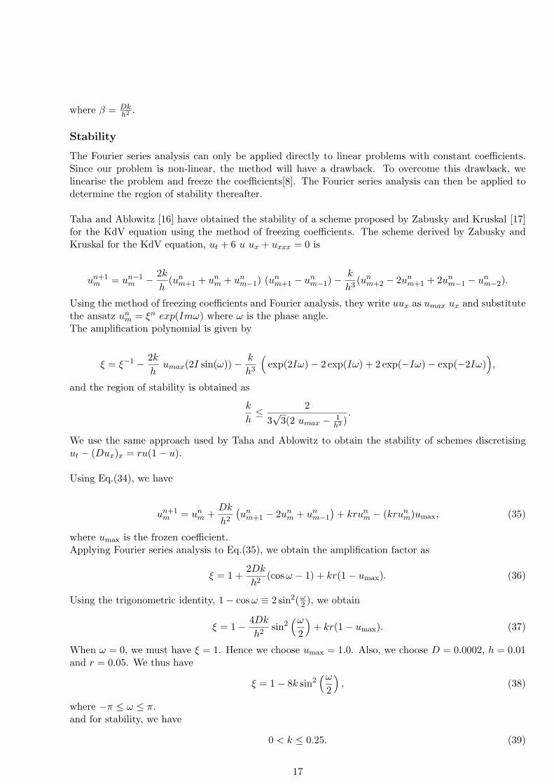
As k → 0 , Eq. (40) reduces to Eq.(3) and so the Upwind Forward Euler finite difference scheme isconsistent.Fig. (10) shows the variation of the modulus of amplification factor for the Upwind Forward Eulerscheme vs phase angle at h = 0.01, with some different values of k. As k increases, for a given angle,the numerical dissipation increases.
0 0.5 1 1.5 2 2.5 30
0.2
0.4
0.6
0.8
1
ω
|ξ|
k = 0.025k = 0.050k = 0.075k = 0.100k = 0.125
(a)
0 0.5 1 1.5 2 2.5 30
0.2
0.4
0.6
0.8
1
ω
|ξ|
k = 0.150k = 0.175k = 0.200k = 0.225k = 0.250
(b)
Figure 10: Plot of modulus of amplification factor for Upwind forward Euler scheme for some values ofk, with h = 0.01, when umax = 1.0.
Spectral Analysis
To study the dispersion of numerical schemes discretising the partial differential equation,
∂u
∂t= 2 α u
∂u
∂x+ γ
∂u
∂x+ ν
∂3u
∂x3, (41)
Asher and McLachlan [4] considered the linearised version of Eq.(41) which is
∂u
∂t= γ
∂u
∂x+ ν
∂3u
∂x3. (42)
We use the same approach that they used. The linearised form of Eq.(3) is given by
∂u
∂t−D
∂2u
∂x2= ru. (43)
We then consider the perturbation
u(x, t) = eαt eIθx. (44)
18
Substituting Eq.(44) in (43) and solving for the dispersion relation, α, we obtain
α = r −Dθ2. (45)
Since the dispersion relation does not have an imaginary part, the relative phase error cannot becomputed using the formula in Eq.(21).
6.2 Non-Standard Finite Difference Scheme
Eq. (3) is approximated by [11]
un+1m − unm
k−D
(unm+1 − 2unm + unm−1
h2
)= runm − r
(unm+1 + unm + unm−1
3
)un+1m ,
which simplifies to
un+1m =
(1 + kr − 2β)unm + β(unm+1 + unm−1)
1 + kr(unm+1+un
m+unm−1
3
) , (46)
where β = Dkh2 .
Stability
Applying the Fourier series analysis and the method of freezing coefficients to Eq.(46), we obtain theamplification factor for the NSFD scheme as
ξ =1 + kr + 2Dk
h2 (cosω − 1)
1 + krumax. (47)
Using the trigonometric identity, 1− cosω ≡ 2 sin2(ω2 ) we have
ξ =1 + kr − 4Dk
h2 sin2(ω2 )
1 + krumax. (48)
When ω = 0, we must have ξ = 1, hence umax is chosen as 1.0.Setting D = 0.0002, r = 0.05, h = 0.01 and umax = 1.0, the amplification factor is given as
ξ =1 + 0.05k − 8k sin2(ω2 )
1 + 0.05k.
For stability, we have
−1 ≤1 + 0.05k − 8k sin2(ω2 )
1 + 0.05k≤ 1.
Since this condition must hold for every phase angle, ω ∈ [−π, π] we have 8k ≤ 2 + 0.1k which givesk ≤ 0.253. Hence the region of stability is given by
0 < k ≤ 0.253.
We note that in [6], they have used k = 0.26 when h is chosen as 0.01. However, from our stabilityanalysis, we observe that the Upwind Forward Euler and NSFD schemes are not stable for k > 0.25and k > 0.253 respectively.
19
Consistency
To obtain the truncation errors of the NSFD scheme, we need to first determine the Taylor expansionof the terms in Eq. (46) about (m,n). Substituting Eqs.(12)-(14) in (46) and simplifying, we have
∂u
∂t−D
∂2u
∂x2= ru(1− u)− rh
3u2 −
(rku+
rkh
3u
)∂u
∂t−(k
2+
k2r
2u+
rk2h
6u
)∂2u
∂t2
−(k2
6+
rk3
6u+
rhk3
18u
)∂3u
∂t3+ · · · (49)
As k → 0 and h → 0, Eq.(49) reduces to Eq. (3) and hence the NSFD scheme is consistent.
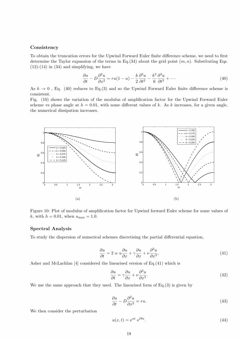
Fig.(11) shows the modulus of amplification factor vs phase angle for the Non-Standard Finite Differencescheme for some values of k, with h = 0.01. It is seen that the scheme is stable for 0 < k ≤ 0.253.
0 0.5 1 1.5 2 2.5 30
0.2
0.4
0.6
0.8
1
ω
|ξ|
k = 0.025k = 0.050k = 0.075k = 0.100k = 0.125
(a)
0 0.5 1 1.5 2 2.5 30
0.2
0.4
0.6
0.8
1
ω
|ξ|
k = 0.150k = 0.175k = 0.200k = 0.225k = 0.250
(b)
Figure 11: Plot of modulus of amplification factor vs ω ∈ [0, π] for Non-Standard Finite Differencescheme for some values of k, with h = 0.01, with umax = 1.0.
The UPFD scheme when used to approximate Eq.(3) is given by [6]
un+1m − unm
k−D
(unm+1 − 2un+1
m + unm−1
h2
)= runm − runmun+1
m ,
which simplifies to
un+1m =
(1 + kr)unm + β(unm+1 + unm−1)
1 + 2β + krunm, where β =
Dk
h2. (50)
Stability
Applying the Fourier series analysis and method of freezing coefficients to Eq.(50), we obtain theamplification factor for the Unconditionally Positive Finite Difference scheme given as
ξ =1 + kr + 2β cosω
1 + 2β + krumax.
20
where β = Dkh2 .
When ω = 0, we must have ξ = 1. Hence umax = 1.0Setting D = 0.0002, r = 0.05, h = 0.01 and umax = 1.0, we have amplification factor given by
ξ =1 + 4k cosω + 0.05k
1 + 4.05k. (51)
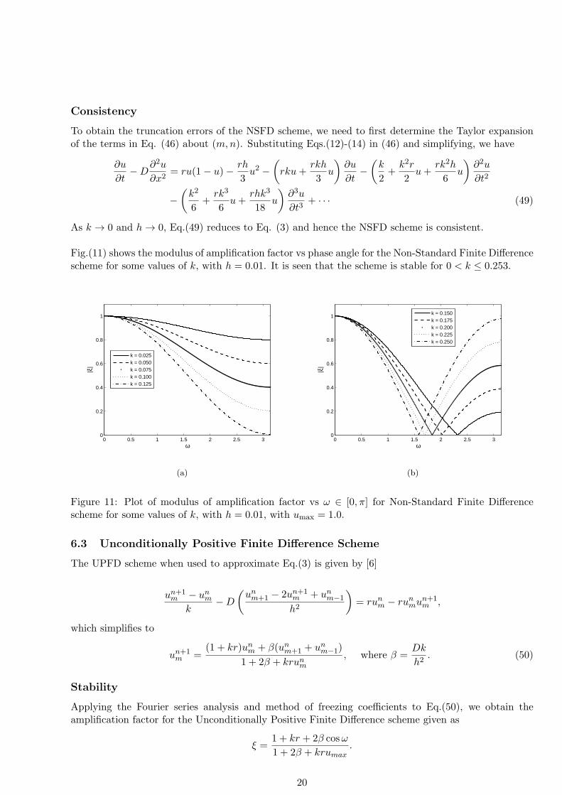
The scheme is unconditionally stable.We note that the UPFD scheme is unconditionally stable while the NSFD and Upwind Forward Eulermethods have almost the same region of stability.
0 0.5 1 1.5 2 2.5 30
0.2
0.4
0.6
0.8
1
ω
|ξ|
Figure 12: Plots of modulus of amplification factor for Unconditionally Positive Finite Difference schemefor k = h3, with h = 0.01.
6.4 Consistency
To obtain the truncation errors for the Unconditionally Positive Finite difference scheme we need tofirst determine the Taylor expansion of the terms in Eq.(50) about (m,n). Substituting Eqs.(12)-(14)in (50) and simplifying we have
∂u
∂t−D
∂2u
∂x2= ru(1− u)−
(kru+
2Dk
h2
)∂u
∂t−(k
2+
Dk2
h2+
k2r
2u
)∂2u
∂t2
−(k2
6+
Dk3
3h2− k3r
6u
)∂3u
∂t3+ · · · (52)
To ensure that the UPFD scheme is consistent, we choose the time step that depends on the spatialstep such that the truncation error reduces to zero. For this reason we let k = h3. Hence, we have
∂u
∂t−D
∂2u
∂x2= ru(1− u)−
(h3ru+ 2Dh
)∂u
∂t− h3
2
(1 + 2Dh+ rh3u
)∂2u
∂t2
− h6
6
(1 + 2Dh+ rh3u
)∂3u
∂t3+ · · · (53)
As h → 0, Eq. (53) reduces to Eq.(3) and so the scheme is consistent.
21
7 Numerical Results for Experiment 2
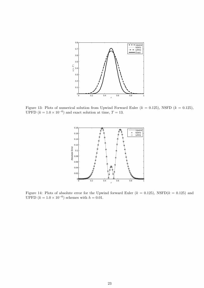
We tabulate the error rate with respect to L1 norm, dissipation, dispersion and total error in Tables (4)to Table (6) for the three numerical schemes. Based on Tables (4) to (6), we observe that dispersionerror is greater than dissipation error at a given value of k for all the three schemes. As k increases,dissipation, dispersion error and total errors are not very much affected.In the case of Upwind Forward Euler finite difference scheme, Enum is smallest when k = 0.125 and thetotal error is least when k = 0.050. In the case of Non-Standard Finite Difference scheme, errors eitherincrease or decrease as k is increased i.e there is no general behaviour. The NSFD scheme performs bestat k = 0.125 with Enum and total error being 5.5968 × 10⁻² and 6.8480 × 10⁻³. The values for Enum
and Total error are 5.6085×10⁻² and 6.8630×10⁻³ respectively for the Unconditionally Positive FiniteDifference scheme when it is consistent with k = 10−6 and h = 0.01 and consequently it took severalhours to obtain the results from the code in Matlab using this scheme.
k No of time steps L1 error Dissipation Error Dispersion Error Total Error
Table 6: Errors for Unconditionally Positive Finite Difference scheme for Problem 2.
22
0 0.2 0.4 0.6 0.8 10
0.1
0.2
0.3
0.4
0.5
0.6
0.7
0.8
x
u(x
,T)
UpwindNSFDUPFDExact
Figure 13: Plots of numerical solution from Upwind Forward Euler (k = 0.125), NSFD (k = 0.125),UPFD (k = 1.0× 10⁻⁶) and exact solution at time, T = 13.
0 0.2 0.4 0.6 0.8 10
0.02
0.04
0.06
0.08
0.1
0.12
0.14
0.16
0.18
x
Abs
olut
e E
rror
UpwindNSFDUPFD
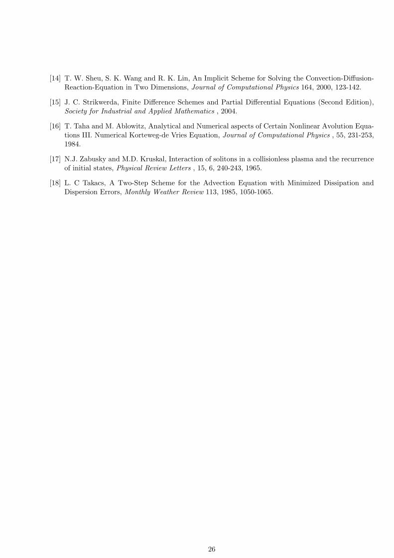
Figure 14: Plots of absolute error for the Upwind forward Euler (k = 0.125), NSFD(k = 0.125) andUPFD (k = 1.0× 10⁻⁶) schemes with h = 0.01.
23
(a) Upwind Forward Euler scheme with k =0.125
(b) NSFD scheme with k = 0.250
(c) UPFD scheme with k = 1.0× 10⁻⁶
Figure 15: Numerical solutions using Upwind Forward Euler, NSFD and UPFD schemes plotted vstime, t ∈ [0, 13] vs space, x ∈ [0, 1].
8 Conclusion
In this paper, three finite difference schemes have been used to solve a linear and a non-linear advection-diffusion-reaction equation, both with constant convective velocity and diffusion. The errors from theNon-Standard Finite Difference scheme are less than that for the Upwind Forward Euler scheme andUnconditionally Positive Finite Difference scheme for the first experiment. For the second experimentwhich models a non-linear diffusion reaction, the errors for the three schemes are not very different ata given value of h and k.The Unconditionally Positive Finite Difference scheme suffers a drawback when it comes to consistency.When spatial step becomes smaller, the computations requires more CPU time and power. This draw-back was experienced in experiment 2 where the number of time steps required was 1.3× 10⁷.In the two cases considered, the velocity was constant, i.e we have a steady fluid flow. However we canalso have transient fluid flow where the velocity can be dependent on time. The analysis of dispersiveand dissipative properties of numerical methods in the case of transient fluid flow can be very compli-cated as we have additional parameters involved. One way to handle transient fluid flow problems is toconsider higher order Nonstandard finite difference schemes such as those used in Anguelov et al. [1] asfirst order methods cannot handle such problems.
24
Acknowledgements
The authors acknowledge the financial support of DST/NRF SARChI chair in Mathematical Modelsand Methods in Bioengineering and BioSciences of the University of Pretoria and would like to thankthe three anonymous reviewers for their very constructive comments and suggestions which have helpedto improve the paper considerably. Dr Appadu is also grateful to the Research Development Programmeof the University of Pretoria for funding.
References
[1] R. Anguelov, P. Kama and J. M. S. Lubuma, On non-standard finite difference models of reaction-diffusion equations, Journal of Computational and Applied Mathematics 175, 2005, 11-29.
[2] A. R. Appadu, Numerical solution of the 1-D advection-diffusion equation using standard andnonstandard finite difference schemes, Journal of Applied Mathematics 15, 2013, 201-215.
[3] A. R. Appadu and M. Z. Dauhoo, The concept of minimized integrated exponential error for lowdispersion and low dissipation, International Journal for Numerical Methods in Fluids 65, 2011,578-601.
[4] M. Ascher and R. McLachlan, On Symplectic and Multisympletic Schemes for the KDV Equation,Journal of Scientific Computing 25, 2005.
[5] R. Liska and B. Wendroff, Composite schemes for Conservation Laws, SIAM Journal on NumericalAnalysis 35, 6, 2250-2271.
[6] B. M. Chen-Charpentier and H. V. Kojouharov, Unconditionally positivity preserving scheme foradvection-diffusion-reaction equations, Mathematical and Computer Modelling 57, 2013, 2177-1285.
[7] B. M. Chen-Charpentier and H. V. Kojouharov, Non-standard Numerical Methods Applied toSubsurface Biobarrier Formation Models in Porous Media, Bulletin of Mathematical Biology 61, 4,1999, 779-798.
[8] D. R. Durran, Numerical Methods for Fluid Dynamics with Applications to Geophysics(SecondEdition), Springer , 2010.
[9] J. M. Makungu, H. Haario and W. C. Mahera, A generalised 1-dimensional particle trans-port method for convection-diffusion-reaction model, African Mathematical Union and Springer-Verlag 23, 2011, 21-39.
[10] R. E. Mickens, Nonstandard finite difference schemes for reaction-diffusion equations, NumericalMethods for Partial Differential Equations 15, 1999, 201-215.
[11] R. E. Mickens, Nonstandard finite difference schemes for reaction-diffusion equations having linearadvection, Numerical Methods for Partial Differential Equations 15, 4, 2000, 361-364.
[12] K. C. Patidar, On the use of nonstandard finite difference methods, Journal of Difference Equationsand Application 11, 2005, 735-758.
[13] A. D. Polyanin and V. F. Zaitsev, Handbook of Nonlinear Partial Differential Equations, Chapman& Hall/CRC , 2004.
25
[14] T. W. Sheu, S. K. Wang and R. K. Lin, An Implicit Scheme for Solving the Convection-Diffusion-Reaction-Equation in Two Dimensions, Journal of Computational Physics 164, 2000, 123-142.
[15] J. C. Strikwerda, Finite Difference Schemes and Partial Differential Equations (Second Edition),Society for Industrial and Applied Mathematics , 2004.
[16] T. Taha and M. Ablowitz, Analytical and Numerical aspects of Certain Nonlinear Avolution Equa-tions III. Numerical Korteweg-de Vries Equation, Journal of Computational Physics , 55, 231-253,1984.
[17] N.J. Zabusky and M.D. Kruskal, Interaction of solitons in a collisionless plasma and the recurrenceof initial states, Physical Review Letters , 15, 6, 240-243, 1965.
[18] L. C Takacs, A Two-Step Scheme for the Advection Equation with Minimized Dissipation andDispersion Errors, Monthly Weather Review 113, 1985, 1050-1065.