Arbitrage-Free Pricing in Nonlinear Market Models (or, Cooking … · 2018-06-19 · Arbitrage-Free...

Arbitrage-Free Pricing in Nonlinear Market

Models

(or, Cooking with Adjustments)

Tomasz R. BieleckiDepartment of Applied MathematicsIllinois Institute of Technology

[email protected]

Joint work with Igor Cialenco and Marek Rutkowski

Modeling, Stochastic Control, Optimization, and Related

Applications

Financial and Economic Applications

IMA

June 11-15, 2018

[email protected]

Outline of the talk:

Motivation

Trading adjustments: a unified approach

No arbitrage for trading desk: elimination of bad market models

Regular market models

Fair prices and other prices

Valuation in regular models through BSDEs

T.R. Bielecki Illinois Tech June 14, 2018 Slide 2

Motivation and Preliminaries

Motivations

Major changes in the operations of financial markets:Defaultability of the counterparties became one of the key problemsof financial management.The classical ‘discounting of future cash flows using the risk-free rate’is no longer accepted; differential funding costs.

In the presence of funding costs, counterparty credit risk, and other

adjustments, the classical arbitrage pricing theory no longer applies.

Non-uniqueness and non-linearity of one-sided prices: asymmetric

pricing rules may fail to yield a mutually acceptable price for

counterparties.

Aggregation of pricing rules: non-linear effects of netting of

exposures and/or margin accounts between two (or more)

counterparties.

Arbitrage opportunities: an OTC contract may introduce arbitrage

opportunities to an arbitrage-free model.

...


Main Goal

To develop a comprehensive no-arbitrage framework for valuation of

contracts in the presence of salient features of real-world trades such as

trading constraints, differential funding costs, collateralization,

counterparty credit risk and capital requirements.

T.R. Bielecki, Igor Cialenco, and M. Rutkowski, Arbitrage-Free Pricing of

Derivatives in Nonlinear Market Models, Probability, Uncertainty and

Quantitative Risk, 2018 vol 3, no. 2


Related works

N. El Karoui and M. C. Quenez (1996). Non-linear pricing theory and BSDEs.

In Financial Mathematics, Lecture Notes in Mathematics 1656, pages 191–246. eds. B.

Biais et al., Springer, Berlin.

Piterbarg, V. (2010) Funding beyond discounting: collateral agreements and

derivatives pricing. Risk Magazine, February, 97–102.

Piterbarg, V. (2012) Cooking with collateral, Risk Magazine, August (2012), 58-63.

T. R. Bielecki and M. Rutkowski (2015) Valuation and hedging of contracts

with funding costs and collateralization, SIAM Fin Math, 6:594–655.

T. Nie and M. Rutkowski (2015) Fair bilateral prices in Bergman’s model. IJTAF,

18:1550048.


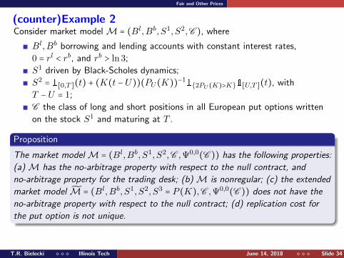
(counter)Example 1

Consider the Black-Scholes model (B,S1) with zero interest rate in which,borrowing of cash is prohibited, and hedger’s initial endowment is 0.

Obviously, the model is arbitrage-free in the classical sense.

The hedger can replicate (without borrowing cash) a short position in aput option maturing at T written on S1. Denote by Pt(K) the fair(Black-Scholes) price of this put option.

The hedger can replicate (without borrowing cash) the contract C that pays

PU(K) at time U , for some fixed U < T and−PT (K) = −(K − S1

T )+, at time T .

The price of this contract is zero.

Extend the market model by introducing the second risky asset

S2t = 1[0,T ](t) + 2K(t −U)(PU(K))

−11[U,T ](t).


Easy to check that (B,S1, S2) is still arbitrage-free if the borrowing

of cash is not allowed; the only way of investing in the second asset

is to sell short the first one.

The price of the contract C based on the concept of replication is

still equal to 0.

However, the hedger who enters into the contract C at time 0 at

zero price has now an arbitrage opportunity. She may now use the

cash amount PU(K) received at time U to buy the asset S2, that

yields the amount 2K(T −U) at time T , which strictly dominates

the hedger’s liability PT (K), assuming that T −U ≥ 0.5.

Similar example can be provided with no trading constrains.

What did go wrong and how to avoid this?


Easy to check that (B,S1, S2) is still arbitrage-free if the borrowing

of cash is not allowed; the only way of investing in the second asset

is to sell short the first one.

The price of the contract C based on the concept of replication is

still equal to 0.

However, the hedger who enters into the contract C at time 0 at

zero price has now an arbitrage opportunity. She may now use the

cash amount PU(K) received at time U to buy the asset S2, that

yields the amount 2K(T −U) at time T , which strictly dominates

the hedger’s liability PT (K), assuming that T −U ≥ 0.5.

Similar example can be provided with no trading constrains.

What did go wrong and how to avoid this?


Notations and main setup Underlying Assets

(Ω,G,G = (Gt)t∈[0,T ],P) a filtered probability space, with a fixed time

horizon T > 0. As usual, all processes are assumed to be G-adapted, and

all semimartingales, to be cadlag.

Risky assets. We denote by S = (S1, . . . , Sd) the ex-dividend prices of

d risky assets with the corresponding cumulative dividend streams

D = (D1, . . . ,Dd).

Examples of ‘Risky Assets’: stocks, sovereign or corporate bonds, stock options,

interest rate swaps, currency options, CDS, CDO ...

Funding accounts. Bi,l will stand for the lending funding account

associated with the ith risky asset. Respectively, Bi,b will be used to

denote the borrowing funding account.

Cash accounts. The riskless lending/borrowing cash account B0,l/b

is used for unsecured lending/borrowing of cash.

If Bi,l = Bi,b, i = 0,1, . . . , d, then we simply write Bi.T.R. Bielecki Illinois Tech June 14, 2018 Slide 8

Financial Contract

We consider financial contracts between two parties - the hedger and

the counterparty. All the cash flows will be viewed from the perspective

of the hedger.

Definition

A bilateral financial contract is a pair C = (A,X ), with A representing

the cumulative (promised) cash flows from time 0 till maturity T , and

X the trading adjustments associated to this contract.


Financial Contract Contractual Cash Flows

The process A models all contractual cash flows of the contract,

either paid out from the wealth or added to the hedger’s wealth.

For example, if the contract stipulates that the hedger will ‘receive’ the

cash flows a1, a2, . . . , am at times t1, t2, . . . , tm ∈ (0, T ], then A is given

by

At =m

∑l=1

1[tl,∞)(t)al.

The price of the contract C exchanged at its initiation is not included in

A, and it is to be determined.

If the contract is initiated at time t, then the remaining cumulative cash

flow is Atu ∶= Au −At.

Example: Hedger sells at time t the European call Si, strike K, maturity T . Then

m = 1, t1 = T , a1 = −(SiT −K)+, and At

u = −(SiT −K)+1[T,∞)(u) for u ∈ [t, T ].


Financial Contract Trading Adjustments

Process X represents the additional features or clauses of a contract, and

is formally given by

X = (X1, . . . ,Xn;α1, . . . , αn;β1, . . . , βn).

Xk is an adjustment (stochastic) process. It may depend on A, the

hedger’s trading strategy, the price of C (to be determined), etc and

vise versa; hence, possible feedback effect.

αkXk is an additional cash flow for the hedger either stipulated in

the clauses of the contract or imposed by a third party (for instance,

the regulator),

remuneration process βk used to determine the net interest

payments associated with Xk.

With proper choice of X , we reconcile: short-selling of risky assets,

repo market trading, collateralization, counterparty credit risk,

regulatory capital, etc.



Example of Adjustment process: CollateralizationThe hedger either receives or pledges collateral with value denoted by C,

and represents the value of the margin account. We take

Ct =X1t +X

2t ∶= C

+

t −C−

t = Ct1Ct≥0 +Ct1Ct<0.

Rehypothecated collateral (the amount received can be used by the

hedger for trading). We set α1t = α

2t = 1, and take β1, β2 to be the

value of banking account with the interest rate paid/recieved on

collateral. Consequently, the ‘cash adjustment’ to the wealth is

Ct − ∫t

0C+

u /β1udβ

1u + ∫

t

0C−

u /β2udβ

2u.

For segregated collateral: α1t = 0, α2

t = 1, and the cash adjustment is

−C−

t − ∫

t

0C+

u /β1udβ

1u + ∫

t

0C−

u /β2udβ

2u.



Composite Contract with Adjustments: Counterparty Risk I

We denote by τh and τ c the default times of the hedger and his

counterparty, respectively.

τ ∶= τh ∧ τ c is the moment of the first default.

We define the random variable Υ as

Υ = Qτ +∆Aτ −Cτ , (5.1)

where Q is the Credit Support Annex (CSA) closeout valuation

process of the contract A, ∆Aτ = Aτ −Aτ− is the jump of A at τ

corresponding to a (possibly null) promised bullet dividend at τ , and

Cτ is the value of the collateral process C at time τ .

In the financial interpretation, Υ+ is the amount the counterparty

owes to the hedger at time τ , whereas Υ− is the amount the hedger

owes to the counterparty at time τ .



Composite Contract with Adjustments: Counterparty Risk II

Definition

The CSA closeout payoff K is defined as

K ∶= Cτ + 1τc<τh(RcΥ

+−Υ−

) + 1τh<τc(Υ

+−RhΥ−

)

+ 1τh=τc(RcΥ

+−RhΥ−

). (5.2)

The counterparty risky cumulative cash flows process A♯ is given by

A♯

t = 1t<τAt + 1t≥τ(Aτ− +K), t ∈ [0, T ]. (5.3)



Composite Contract with Adjustments: Counterparty Risk III

Definition

By the CCR processes, we mean the processes CL,CG and RP where

the credit loss CL equals

CLt = −1t≥τ1τ=τc(1 −Rc)Υ+,

the credit gain CG equals

CGt = 1t≥τ1τ=τh(1 −Rh)Υ

−,

and the replacement process is given by

CRt = 1t≥τ(Aτ −At +Qτ).

The CCR cash flow is given by ACCR = CL +CG +CR.



Composite Contract with Adjustments: Counterparty Risk IV

Let X = (X1,X2) = (C+,−C−).

Proposition

The counterparty risky and collateralized contract (A♯,X ) admits the

following formal decompositions

(A♯,X ) = (A,X ) + (ACCR,0)

and

(A♯,X ) = (A,0) + (ACCR,X ).



Composite Contract with Adjustments: Counterparty Risk V

Remark

We may interpret the counterparty risky contract as the clean contract

A, which is complemented by the following adjustment processes:

the collateral adjustment processes: X1 = C+ and X2 = −C−,

the CCR adjustment processes: X3 = CL, X4 = CG and X5 = CR.

Specifically, we have that

A♯

t = At +5

∑k=3

Xkt , t ∈ [0, T ].


Self Financing Condition

Portfolios

Definition

An portfolio on the time interval [t, T ] is an R3d+2-valued, G-adapted

process

ϕt = ( ξ1, . . . , ξd

´¹¹¹¹¹¹¹¹¹¹¹¹¹¹¹¹¸¹¹¹¹¹¹¹¹¹¹¹¹¹¹¹¹¹¶risky assets

; ψ0,l, ψ0,b

´¹¹¹¹¹¹¹¹¹¹¹¹¹¹¸¹¹¹¹¹¹¹¹¹¹¹¹¹¹¶cash account

, ψ1,l, ψ1,b, . . . , ψd,l, ψd,b

´¹¹¹¹¹¹¹¹¹¹¹¹¹¹¹¹¹¹¹¹¹¹¹¹¹¹¹¹¹¹¹¹¹¹¹¹¹¹¹¹¹¹¹¹¹¹¹¹¹¹¹¹¹¹¹¹¹¹¹¹¹¹¹¹¹¹¸¹¹¹¹¹¹¹¹¹¹¹¹¹¹¹¹¹¹¹¹¹¹¹¹¹¹¹¹¹¹¹¹¹¹¹¹¹¹¹¹¹¹¹¹¹¹¹¹¹¹¹¹¹¹¹¹¹¹¹¹¹¹¹¹¹¹¶funding accounts

),

where the components represent the positions in risky assets

(Si,Di), i = 1, . . . , d, cash accounts B0,l, B0,b, and funding accounts

Bi,l,Bi,b, i = 1, . . . , d for risky assets.

Throughout we assume that ψi,lt ≥ 0, ψi,b

t ≤ 0 and ψi,lt ψ

i,bt = 0, for all

i = 0,1, . . . , d and t ∈ [0, T ].

Portfolio may have some explicit constrains.



xt represents the hedger’s endowment of at time t ∈ [0, T )

pt stands for the price at time t of Ct = (At,X t)

Definition

The portfolio value corresponding to the trading strategy ϕ is defined as

V pu (xt, pt, ϕ

t,Ct) ∶=d

∑i=1

ξiuSiu +

d

∑j=0

(ψj,lu Bj,lu + ψj,bu Bj,b

u ) .

Correspondingly, the adjusted gains process is given by

Gu(xt, pt, ϕt,Ct) ∶=

d

∑i=1∫

u

tξiv (dS

iv + dD

iv) +

d

∑j=0∫

u

t(ψj,lv dBj,l

v + ψj,bv dBj,bv )

+n

∑k=1

αkuXku −

n

∑k=1∫

u

tXkv (β

kv )

−1 dβkv +Atu.



Definition

(xt, pt, ϕt,Ct) is a self-financing trading strategy on [t, T ] if

V pu (xt, pt, ϕ

t,Ct) = xt + pt +Gu(xt, pt, ϕt,Ct), u ∈ [t, T ].

Note that

V p0 (x, p,ϕ,C) =

d

∑i=1

ξi0Si0 +

d

∑j=0

(ψj,l0 Bj,l0 + ψj,b0 Bj,b

0 ) = x + p +n

∑k=1

αk0Xk0 .

In contrast to classical theory, in nonlinear market models, the initial

endowment x, the initial price p and the adjustment cash flows of a

contract may all affect the dynamics of the gains process.



Definition

The market model is the quintuplet M = (S,D,B,C ,Φ(C )) where

Φ(C ) stands for the set of all self-financing trading strategies associated

with the class C of contracts.



Discount Factor: for any x ∈ R, we denote by

Bt(x) ∶= 1x≥0B0,lt + 1

x<0B0,bt .

The symbol will be used for discounting, e.g. V = V /B.

Assumption:

(i) for any initial endowment x ∈ R of the hedger, the null contract

N = (0,0) belongs to C .

(ii) for any x ∈ R, the trading strategy (x,0, ϕ,N ), where all

components of ϕ vanish except for either ψ0,l, if x ≥ 0, or ψ0,b, if

x < 0, is ‘feasible’ and

V pt (x,0, ϕ,N ) = Vt(x,0, ϕ,N ) = xBt(x), t ∈ [0, T ].

This assumption is needed: to insure that the zero contract has zero fair

price; serves as a benchmark to assess the gains/losses.


Arbitrage-free property Primary Arbitrage

Definition

An arbitrage opportunity with respect to the null contract in market

model M, or a primary arbitrage opportunity, for the hedger with an

initial endowment x is a strategy (x,0, ϕ,N ) such that

P(VT (x,0, ϕ,N ) ≥ x) = 1, P(VT (x,0, ϕ,N ) > x) > 0.

If no primary arbitrage opportunity exists in M, then M is arbitrage free

with respect to the null contract.

This no-arbitrage property is not strong enough for developing

reasonable pricing frameworks.



Definition

For a contract C = (A,X ) and an initial endowment x, the combined

wealth is defined as

V com(x1, x2, ϕ, ϕ,A,X ,Y) ∶= V (x1,0, ϕ,A,X ) + V (x2,0, ϕ,−A,Y),

(7.1)

where x1 + x2 = x.

Definition

A pair (x1, ϕ;x2, ϕ) is an arbitrage opportunity for the trading desk

with respect to a contract (A,X ) if

P(V comT (x1, x2, ϕ, ϕ,A,X ,Y) ≥ x) = 1, P(V com

T (x1, x2, ϕ, ϕ,A,X ,Y) > x) > 0.

Market model M = (S,D,B,C ) has the no-arbitrage property for the

trading desk if there are no arbitrage opportunities for the trading desk

with respect to any contract C from C .



No-arbitrage for trading desk is stronger than no-arbitrage with

respect to the null contract.

These definitions of arbitrage are meant to eliminate bad market

models.

The market model (B,S1, S2,C) from (counter)Example 1 is

arbitrage free with respect to the null contract, and admits arbitrage

opportunity for the trading desk.

One can derive interesting dynamics for V com, and provide sufficient

conditions for the trading-desk no arbitrage, in particular expressed

in terms of the existence of a (super-)martingale measure.


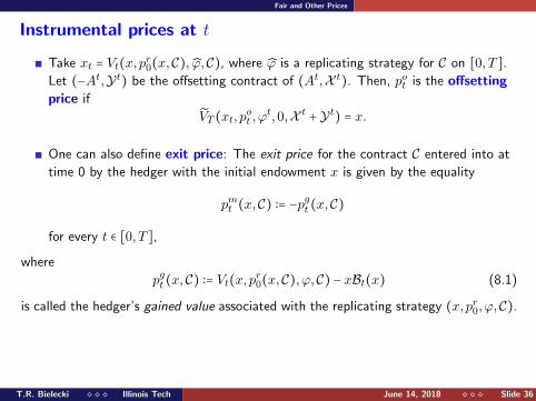
Fair and Other Prices

Part II: Fair and Other Pricing



Ct will denote a class of contracts, and Ψt,xt(Ct) the set of all ‘feasible’

trading strategies.

Definition

A trading strategy (xt, pt, ϕt,Ct) ∈ Ψt,xt(C ) is a hedger’s pricing

arbitrage opportunity on [t, T ] associated with a contract Ct traded at

pt at time t if

P(VT (xt, pt, ϕt,Ct) ≥ xt) = 1´¹¹¹¹¹¹¹¹¹¹¹¹¹¹¹¹¹¹¹¹¹¹¹¹¹¹¹¹¹¹¹¹¹¹¹¹¹¹¹¹¹¹¹¹¹¹¹¹¹¹¹¹¹¹¹¹¹¹¹¹¹¹¹¹¹¹¹¹¹¹¹¹¹¹¹¹¹¹¹¹¹¹¹¹¹¹¹¹¸¹¹¹¹¹¹¹¹¹¹¹¹¹¹¹¹¹¹¹¹¹¹¹¹¹¹¹¹¹¹¹¹¹¹¹¹¹¹¹¹¹¹¹¹¹¹¹¹¹¹¹¹¹¹¹¹¹¹¹¹¹¹¹¹¹¹¹¹¹¹¹¹¹¹¹¹¹¹¹¹¹¹¹¹¹¹¹¹¹¶

superhedging

and P(VT (xt, pt, ϕt,Ct) > xt) > 0

´¹¹¹¹¹¹¹¹¹¹¹¹¹¹¹¹¹¹¹¹¹¹¹¹¹¹¹¹¹¹¹¹¹¹¹¹¹¹¹¹¹¹¹¹¹¹¹¹¹¹¹¹¹¹¹¹¹¹¹¹¹¹¹¹¹¹¹¹¹¹¹¹¹¹¹¹¹¹¹¹¹¹¹¹¹¹¹¹¹¹¹¹¹¹¹¹¹¹¹¹¹¹¹¹¹¹¹¹¹¹¹¹¹¹¹¹¹¹¹¹¹¹¹¹¹¹¹¹¹¹¹¹¹¹¹¹¹¹¹¹¹¹¹¹¹¹¹¹¹¹¹¹¹¹¹¹¹¹¹¹¹¹¹¹¹¹¹¹¹¹¹¹¹¹¹¹¹¹¹¹¹¹¹¹¹¹¹¹¹¹¹¹¹¹¹¹¹¹¹¹¹¹¹¹¹¹¹¹¹¹¹¹¹¹¹¹¹¹¹¹¹¹¹¹¹¹¹¹¹¹¸¹¹¹¹¹¹¹¹¹¹¹¹¹¹¹¹¹¹¹¹¹¹¹¹¹¹¹¹¹¹¹¹¹¹¹¹¹¹¹¹¹¹¹¹¹¹¹¹¹¹¹¹¹¹¹¹¹¹¹¹¹¹¹¹¹¹¹¹¹¹¹¹¹¹¹¹¹¹¹¹¹¹¹¹¹¹¹¹¹¹¹¹¹¹¹¹¹¹¹¹¹¹¹¹¹¹¹¹¹¹¹¹¹¹¹¹¹¹¹¹¹¹¹¹¹¹¹¹¹¹¹¹¹¹¹¹¹¹¹¹¹¹¹¹¹¹¹¹¹¹¹¹¹¹¹¹¹¹¹¹¹¹¹¹¹¹¹¹¹¹¹¹¹¹¹¹¹¹¹¹¹¹¹¹¹¹¹¹¹¹¹¹¹¹¹¹¹¹¹¹¹¹¹¹¹¹¹¹¹¹¹¹¹¹¹¹¹¹¹¹¹¹¹¹¹¹¹¹¹¹¹¶strict superhedging

.

(xt, pt, ϕt,Ct) ∈ Ψt,xt(C ) is not a hedger’s pricing arbitrage opportunity

if either

P(VT (xt, pt, ϕt,Ct) = xt) = 1 or P(VT (xt, pt, ϕt,Ct) < xt) > 0´¹¹¹¹¹¹¹¹¹¹¹¹¹¹¹¹¹¹¹¹¹¹¹¹¹¹¹¹¹¹¹¹¹¹¹¹¹¹¹¹¹¹¹¹¹¹¹¹¹¹¹¹¹¹¹¹¹¹¹¹¹¹¹¹¹¹¹¹¹¹¹¹¹¹¹¹¹¹¹¹¹¹¹¹¹¹¹¹¸¹¹¹¹¹¹¹¹¹¹¹¹¹¹¹¹¹¹¹¹¹¹¹¹¹¹¹¹¹¹¹¹¹¹¹¹¹¹¹¹¹¹¹¹¹¹¹¹¹¹¹¹¹¹¹¹¹¹¹¹¹¹¹¹¹¹¹¹¹¹¹¹¹¹¹¹¹¹¹¹¹¹¹¹¹¹¹¹¹¶

hedger’s loss condition

.



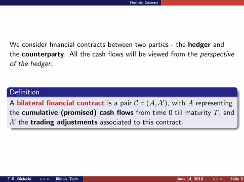
Definition

We say that pft = pft (xt,C

t) is a fair hedger’s price at time t for Ct if

there is no hedger’s pricing arbitrage opportunity (xt, pft , ϕ

t,Ct).

pft such that the loss condition holds for every trading strategy

(xt, pft , ϕ

t,Ct) ∈ Ψt,xt(C ) is called a loss-generating cost.

Hft (xt,C

t) = pft ∈ Gt ∣ p

ft is a fair hedger’s price for Ct

pft (xt,Ct) = ess supHft (xt,C

t)

Hlt(xt,C

t) = plt ∈ Gt ∣ p

lt is a loss-generating cost for Ct

plt(xt,Ct) = ess supHlt(xt,C

t)

Hst (xt,C

t) = pst ∈ Gt ∣ p

st is a superhedging cost for Ct

pst(xt,C

t) = ess infHst (xt,C

t)

Hat (xt,C

t) = pat ∈ Gt ∣ p

at is a strict superhedging cost for Ct

pat(xt,C

t) = ess infHat (xt,C

t)



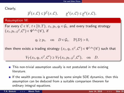
Clearly,

pl(x,C) ≤ pf(x,C), ps(x,C) ≤ pa(x,C),

Assumption M:

For every C ∈ C , t ∈ [0, T ), xt, pt, qt ∈ Gt, and every trading strategy

(xt, pt, ϕt,Ct) ∈ Ψt,xt(C ), if

qt ≥ pt, on D ∈ Gt, P(D) > 0,

then there exists a trading strategy (xt, qt, ψt,Ct) ∈ Ψt,xt(C ) such that

VT (xt, qt, ψt,Ct) ≥ VT (xt, pt, ϕ

t,Ct), on D.

This non-trivial assumption usually is not postulated in the existingliterature.

If the wealth process is governed by some simple SDE dynamics, then thisassumption can be deduced from a suitable comparison theorem forordinary integral equations.



Theorem

Under Assumption M, we have that

plt(xt,Ct) = ps

t(xt,C

t) ≤ pft (xt,C

t) = pa

t(xt,C

t).

If in addition VT (xt, qt, ψt,Ct) > VT (xt, pt, ϕ

t,Ct) on D′ ⊂D, then

plt(xt,Ct) = ps

t(xt,C

t) = pft (xt,C

t) = pa

t(xt,C

t).



Definition

A trading strategy (xt, prt , ϕ

t,Ct) replicates the contract Ct on [t, T ], if

VT (xt, prt , ϕ

t,Ct) = xt,

and the real number prt = prt (xt,C

t) is called the hedger’s replication cost

for Ct at time t.

The replication cost prt is not unique, in general.

If Assumption M holds, then any p ∈ (plt, pat) is a replication cost and a fair

price for Ct.



In a nonlinear market model, that meets the no-arbitrage property

with respect to the null contract (or even the no-arbitrage property

for the trading desk), a replication cost may fail to be a fair hedger’s

price.

Thus ⇒ regular models, under which the cost of replication is

never higher than the minimal cost of superhedging and, the

cost of replication is a fair hedger’s price.



Definition

We say that the market model M = (S,D,B,C ,Ψt,xt(C )) is regular on

[t, T ] with respect to C if Assumption M is met and for every

replicable contract C ∈ C and for any replicating strategy (x, pr0(x), ϕ,X )

the following properties hold:

(i) if pt ∈ Gt and there exists (xt, pt, ϕt,Ct) such that

P(VT (xt, pt, ϕt,Ct) ≥ xt) = 1,

then pt ≥ prt (xt,C

t);

(ii) if pt ∈ Gt and there exists (xt, pt, ϕt,Ct) such that for some D ∈ Gt

P(1DVT (xt, pt, ϕt,Ct) ≥ 1Dxt) = 1, P(1DVT (xt, pt, ϕ

t,Ct) > 1Dxt) > 0,

then P(1D pt > 1Dprt (xt,Ct)) > 0.



(counter)Example 2Consider market model M = (Bl,Bb, S1, S2,C ), where

Bl,Bb borrowing and lending accounts with constant interest rates,

0 = rl < rb, and rb > ln 3;

S1 driven by Black-Scholes dynamics;

S2 = 1[0,T ](t) + (K(t −U))(PU(K))−112PU (K)>K1[U,T ](t), with

T −U = 1;

C the class of long and short positions in all European put options written

on the stock S1 and maturing at T .

Proposition

The market model M = (Bl,Bb, S1, S2,C ,Ψ0,0(C )) has the following properties:

(a) M has the no-arbitrage property with respect to the null contract, and

no-arbitrage property for the trading desk; (b) M is nonregular; (c) the extended

market model M = (Bl,Bb, S1, S2, S3 = P (K),C ,Ψ0,0(C )) does not have the

no-arbitrage property with respect to the null contract; (d) replication cost for

the put option is not unique.



Theorem

Let market model M = (S,D,B,C ,Ψt,xt(C )) be regular on [t, T ] with respect to C .

Then for every contract C ∈ C that can be replicated on [t, T ] we have:

the replication cost prt is unique.

prt (xt,C) = pft (xt,C) = p

lt(xt,C) = p

st(xt,C) = p

at(xt,C).

Even though, in regular model prt is unique, one has to specify the endowment xt.

If the hedger starts at time t = 0 with the endowment x, what is a suitable choice

for xt?Different choices of xt will yield different price processes:

A natural choice is xt = xt(x) ∶= xBt(x), i.e. the hedger has not been dynamicallyhedging the contract between time 0 and time t. Then pet ∶= p

rt (xt(x),C

t) is calledthe hedger’s ex-dividend price at time t of the contract Ct.



Instrumental prices at t

Take xt = Vt(x, pr0(x,C), ϕ,C), where ϕ is a replicating strategy for C on [0, T ].

Let (−At,Yt) be the offsetting contract of (At,X t). Then, pot is the offsetting

price if

VT (xt, pot , ϕ

t,0,X t +Yt) = x.

One can also define exit price: The exit price for the contract C entered into at

time 0 by the hedger with the initial endowment x is given by the equality

pmt (x,C) ∶= −pgt (x,C)

for every t ∈ [0, T ],

where

pgt (x,C) ∶= Vt(x, pr0(x,C), ϕ,C) − xBt(x) (8.1)

is called the hedger’s gained value associated with the replicating strategy (x, pr0, ϕ,C).



Assume that x ≥ 0, and Bi,l = Bi,b = Bi for i = 1, . . . , d. Define

Si,cldt (x) ∶= (Bt(x))−1Sit + ∫

t

0(Bu(x))

−1 dDiu.

The theorem below gives the BSDE for the gained value.

Theorem

Assume that a trading strategy (x, pr0, ϕ,C) replicates C. Then

Y ∶= (B0,l)−1V (x, pr0, ϕ,C) and Zi ∶= Bi,lξi satisfy the BSDE

dYt =d

∑i=1

Zit dSi,cldt − (B0,b

t )−1

(YtB0,lt +

n

∑k=1

αktXkt )

−

dB0,b,lt

+ (B0,lt )

−1 dAt −n

∑k=1

Xkt dβ

k,lt +

n

∑k=1

(1 − αkt )Xkt d(B

0,lt )

−1

with the terminal condition YT = x.

Similar BSDEs can be derived for ex-dividend price, offsetting price, exit price ...


Back to CCR

Recall that the counterparty risky contract (A♯,X ) admits the

following decomposition

(A♯,X ) = (A,X ) + (ACCR,0), (9.1)

Question: can we disentangle the counterparty risk-free valuation of

a credit risky contract from the CRR valuation?

We have the following BSDE for the full contract (A♯,X )

dYt =d

∑i=1

Zit dSi,cldt − (B0,b

t )−1

(YtB0,lt +

n

∑k=1

αktXkt )

−

dB0,b,lt

+ (B0,lt )

−1 dA♯

t −n

∑k=1

Xkt dβ

k,lt +

n

∑k=1


0,lt )

−1

(9.2)

with the terminal condition Yτ = x.


Back to CCR

Let x = x1 + x2 be an arbitrary split of the hedger’s endowment.

Then we obtain the following BSDE corresponding to the

counterparty risk-free contract (A,X )

dY 1t =

d

∑i=1

Z1,it dSi,cldt − (B0,b

t )−1

(Y 1t B

0,lt +

n

∑k=1

αktXkt )

−

dB0,b,lt

+ (B0,lt )

−1 dAt −n

∑k=1

Xkt dβ

k,lt +

n

∑k=1


0,lt )

−1

(9.3)

with Y 1T = x1.

The BSDE associated with the CRR component (ACCR,0) reads

dY 2t =

d

∑i=1

Z2,it dSi,cldt − (B0,b

t )−1(Y 2

t B0,lt )

−

dB0,b,lt + (B0,l

t )−1 dACRR

t

(9.4)

with Y 2τ = x2.


Back to CCR

The question formulated above can now be restated as follows:

under which conditions the equality Y0 = Y10 + Y 2

0 holds for solutions

to BSDEs (9.2), (9.3) and (9.4), so that the three replication costs

satisfy the following equality

pr0(x,A♯,X ) = pr0(x1,A,X ) + pr0(x2,A

CCR,0),

which formally corresponds to decomposition (9.1) of the full

contract and the split x = x1 + x2 of the hedger’s initial endowment?

Study of this question in the general non-linear framework requires

further work.


Thank You !

The end of the talk ...but not of the story

Date post:	01-Apr-2020
Category:	Documents
Upload:	others
View:	9 times
Download:	1 times

Arbitrage-Free Pricing in Nonlinear Market Models (or, Cooking … · 2018-06-19 · Arbitrage-Free...

Documents