EECS 262a Advanced Topics in Computer Systems Lecture 17 Comparison of Parallel DB, CS, MR and Jockey October 30 th , 2013 John Kubiatowicz and Anthony D. Joseph Electrical Engineering and Computer Sciences University of California, Berkeley http://www.eecs.berkeley.edu/~kubitron/cs262 10/30/2013 2 Cs262a-F13 Lecture-17 Today’s Papers • A Comparison of Approaches to Large-Scale Data Analysis Andrew Pavlo, Erik Paulson, Alexander Rasin, Daniel J. Abadi, David J. DeWitt, Samuel Madden, Michael Stonebraker. Appears in Proceedings of the ACM SIGMOD International Conference on Management of Data, 2009 • Jockey: Guaranteed Job Latency in Data Parallel Clusters Andrew D. Ferguson, Peter Bodik, Srikanth Kandula, Eric Boutin, and Rodrigo Fonseca. Appears in Proceedings of the European Professional Society on Computer Systems (EuroSys), 2012 • Thoughts? 10/30/2013 3 Cs262a-F13 Lecture-17 Two Approaches to Large-Scale Data Analysis • “Shared nothing” • MapReduce – Distributed file system – Map, Split, Copy, Reduce – MR scheduler • Parallel DBMS – Standard relational tables, (physical location transparent) – Data are partitioned over cluster nodes – SQL – Join processing: T1 joins T2 » If T2 is small, copy T2 to all the machines » If T2 is large, then hash partition T1 and T2 and send partitions to different machines (this is similar to the split-copy in MapReduce) – Query Optimization – Intermediate tables not materialized by default 10/30/2013 4 Cs262a-F13 Lecture-17 Architectural Differences Parallel DBMS MapReduce Schema Support O X Indexing O X Programming Model Stating what you want (SQL) Presenting an algorithm (C/C++, Java, …) Optimization O X Flexibility Spotty UDF Support Good Fault Tolerance Not as Good Good Node Scalability <100 >10,000
Transcript
EECS 262a Advanced Topics in Computer Systems
Lecture 17
Comparison of Parallel DB, CS, MRand Jockey
October 30th, 2013John Kubiatowicz and Anthony D. Joseph
Electrical Engineering and Computer SciencesUniversity of California, Berkeley
http://www.eecs.berkeley.edu/~kubitron/cs262
10/30/2013 2Cs262a-F13 Lecture-17
Today’s Papers• A Comparison of Approaches to Large-Scale Data Analysis
Andrew Pavlo, Erik Paulson, Alexander Rasin, Daniel J. Abadi, David J. DeWitt, Samuel Madden, Michael Stonebraker. Appears in Proceedings of the ACM SIGMOD International Conference on Management of Data, 2009
• Jockey: Guaranteed Job Latency in Data Parallel ClustersAndrew D. Ferguson, Peter Bodik, Srikanth Kandula, Eric Boutin, and Rodrigo Fonseca. Appears in Proceedings of the European Professional Society on Computer Systems (EuroSys), 2012
• Thoughts?
10/30/2013 3Cs262a-F13 Lecture-17
Two Approaches to Large-Scale Data Analysis• “Shared nothing”• MapReduce
• Parallel DBMS– Standard relational tables, (physical location transparent)– Data are partitioned over cluster nodes– SQL– Join processing: T1 joins T2
» If T2 is small, copy T2 to all the machines» If T2 is large, then hash partition T1 and T2 and send partitions to
different machines (this is similar to the split-copy in MapReduce)– Query Optimization– Intermediate tables not materialized by default
10/30/2013 4Cs262a-F13 Lecture-17
Architectural Differences
Parallel DBMS MapReduce
Schema Support O X
Indexing O X
Programming Model Stating what you want(SQL)
Presenting an algorithm(C/C++, Java, …)
Optimization O X
Flexibility Spotty UDF Support Good
Fault Tolerance Not as Good Good
Node Scalability <100 >10,000
10/30/2013 5Cs262a-F13 Lecture-17
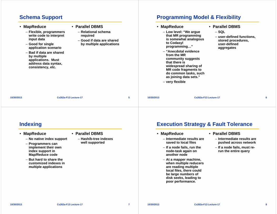
Schema Support• MapReduce
– Flexible, programmers write code to interpret input data
– Good for single application scenario
– Bad if data are shared by multiple applications. Must address data syntax, consistency, etc.
• Parallel DBMS– Relational schema
required– Good if data are shared
by multiple applications
10/30/2013 6Cs262a-F13 Lecture-17
Programming Model & Flexibility• MapReduce
– Low level: “We argue that MR programming is somewhat analogous to Codasylprogramming…”
– “Anecdotal evidence from the MR community suggests that there is widespread sharing of MR code fragments to do common tasks, such as joining data sets.”
– very flexible
• Parallel DBMS– SQL– user-defined functions,
stored procedures, user-defined aggregates
10/30/2013 7Cs262a-F13 Lecture-17
Indexing• MapReduce
– No native index support– Programmers can
implement their own index support in Map/Reduce code
– But hard to share the customized indexes in multiple applications
• Parallel DBMS– Hash/b-tree indexes
well supported
10/30/2013 8Cs262a-F13 Lecture-17
Execution Strategy & Fault Tolerance• MapReduce
– Intermediate results are saved to local files
– If a node fails, run the node-task again on another node
– At a mapper machine, when multiple reducers are reading multiple local files, there could be large numbers of disk seeks, leading to poor performance.
• Parallel DBMS– Intermediate results are
pushed across network– If a node fails, must re-
run the entire query
10/30/2013 9Cs262a-F13 Lecture-17
Avoiding Data Transfers• MapReduce
– Schedule Map to close to data
– But other than this, programmers must avoid data transfers themselves
• Parallel DBMS– A lot of optimizations– Such as determine
where to perform filtering
10/30/2013 10Cs262a-F13 Lecture-17
Node Scalability• MapReduce
– 10,000’s of commodity nodes
– 10’s of Petabytes of data
• Parallel DBMS– <100 expensive nodes– Petabytes of data
10/30/2013 11Cs262a-F13 Lecture-17
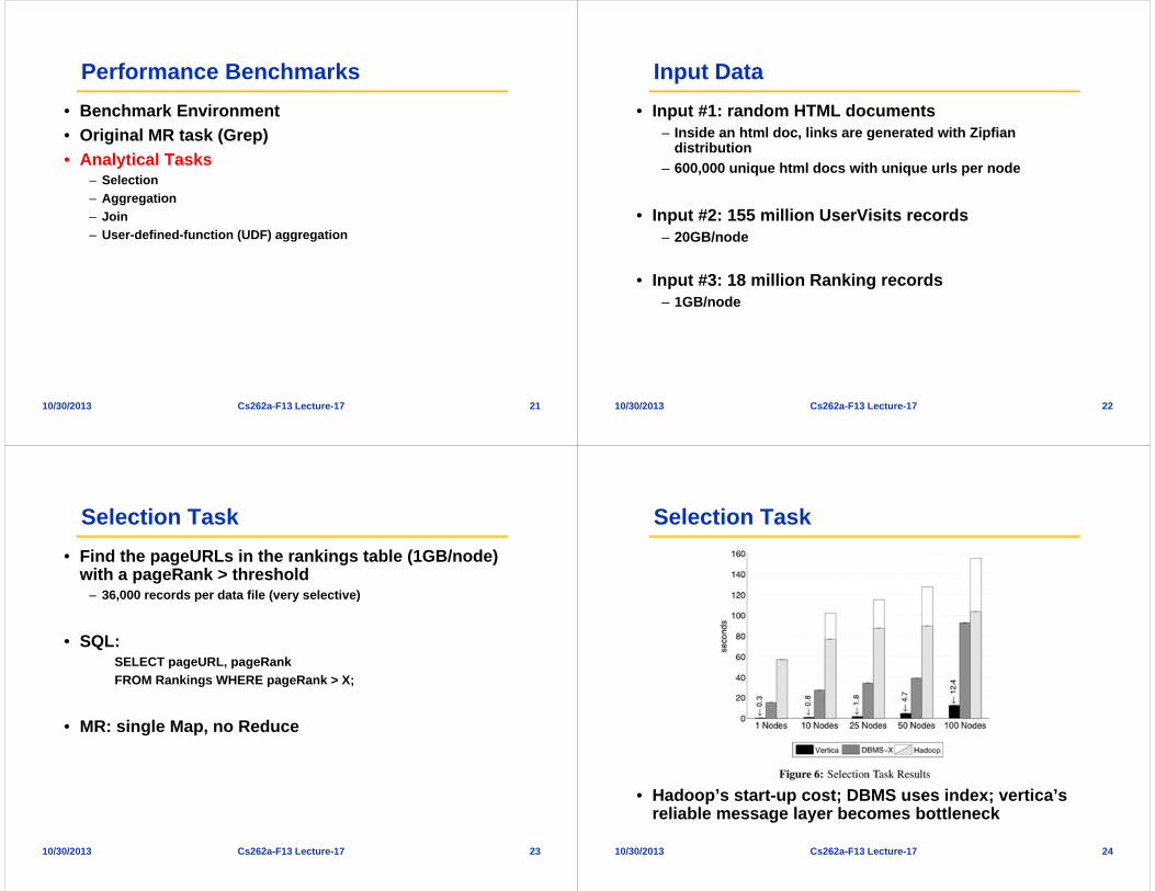
Performance Benchmarks• Benchmark Environment• Original MR task (Grep)• Analytical Tasks
• 100-node cluster– Each node: 2.40GHz Intel Core 2 Duo, 64-bit red hat
enterprise Linux 5 (kernel 2.6.18) w/ 4Gb RAM and two 250GB SATA HDDs.
• Nodes interconnected with Cisco Catalyst 3750E 1Gb/s switches
– Internal switching fabric has 128Gbps– 50 nodes per switch
• Multiple switches interconnected via 64Gbps Cisco StackWise ring
– The ring is only used for cross-switch communications.
10/30/2013 13Cs262a-F13 Lecture-17
Tested Systems• Hadoop (0.19.0 on Java 1.6.0)
– HDFS data block size: 256MB– JVMs use 3.5GB heap size per node– “Rack awareness” enabled for data locality– Three replicas w/o compression: Compression or fewer replicas in
HDFS does not improve performance
• DBMS-X (a parallel SQL DBMS from a major vendor)– Row store– 4GB shared memory for buffer pool and temp space per node– Compressed table (compression often reduces time by 50%)
• Vertica– Column store– 256MB buffer size per node– Compressed columns by default
10/30/2013 14Cs262a-F13 Lecture-17
Benchmark Execution• Data loading time:
– Actual loading of the data– Additional operations after the loading, such as compressing or
building indexes
• Execution time– DBMS-X and vertica:
» Final results are piped from a shell command into a file– Hadoop:
» Final results are stored in HDFS» An additional Reduce job step to combine the multiple files into a
single file
10/30/2013 15Cs262a-F13 Lecture-17
Performance Benchmarks• Benchmark Environment• Original MR task (Grep)• Analytical Tasks
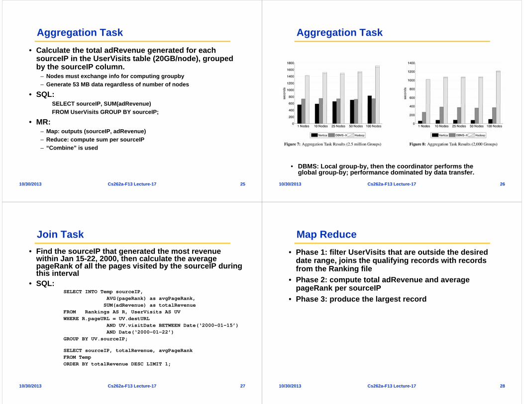
Aggregation Task• Calculate the total adRevenue generated for each
sourceIP in the UserVisits table (20GB/node), grouped by the sourceIP column.
– Nodes must exchange info for computing groupby– Generate 53 MB data regardless of number of nodes
• SQL:SELECT sourceIP, SUM(adRevenue)FROM UserVisits GROUP BY sourceIP;
• MR: – Map: outputs (sourceIP, adRevenue)– Reduce: compute sum per sourceIP– “Combine” is used
10/30/2013 26Cs262a-F13 Lecture-17
Aggregation Task
• DBMS: Local group-by, then the coordinator performs the global group-by; performance dominated by data transfer.
10/30/2013 27Cs262a-F13 Lecture-17
Join Task• Find the sourceIP that generated the most revenue
within Jan 15-22, 2000, then calculate the average pageRank of all the pages visited by the sourceIP during this interval
• SQL:SELECT INTO Temp sourceIP,
AVG(pageRank) as avgPageRank,SUM(adRevenue) as totalRevenue
FROM Rankings AS R, UserVisits AS UVWHERE R.pageURL = UV.destURL
AND UV.visitDate BETWEEN Date(‘2000-01-15’)AND Date(‘2000-01-22’)
GROUP BY UV.sourceIP;SELECT sourceIP, totalRevenue, avgPageRankFROM TempORDER BY totalRevenue DESC LIMIT 1;
10/30/2013 28Cs262a-F13 Lecture-17
Map Reduce• Phase 1: filter UserVisits that are outside the desired
date range, joins the qualifying records with records from the Ranking file
• Phase 2: compute total adRevenue and average pageRank per sourceIP
• Phase 3: produce the largest record
10/30/2013 29Cs262a-F13 Lecture-17
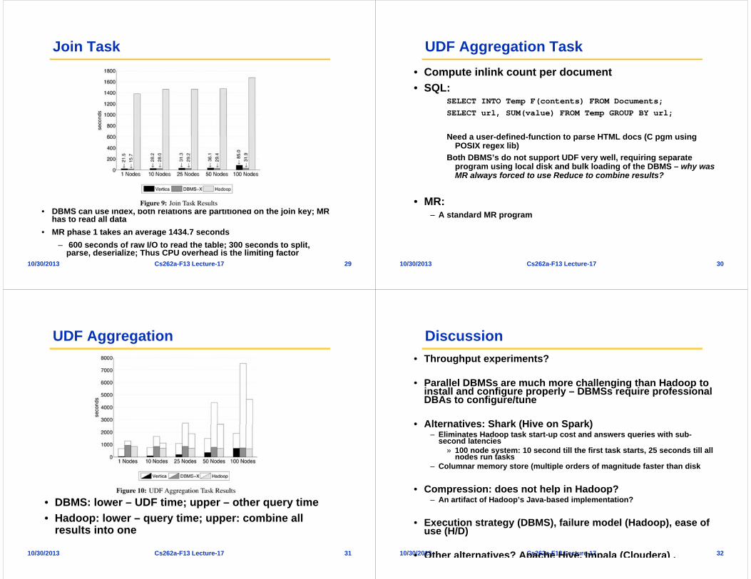
Join Task
• DBMS can use index, both relations are partitioned on the join key; MR has to read all data
• MR phase 1 takes an average 1434.7 seconds– 600 seconds of raw I/O to read the table; 300 seconds to split,
parse, deserialize; Thus CPU overhead is the limiting factor10/30/2013 30Cs262a-F13 Lecture-17
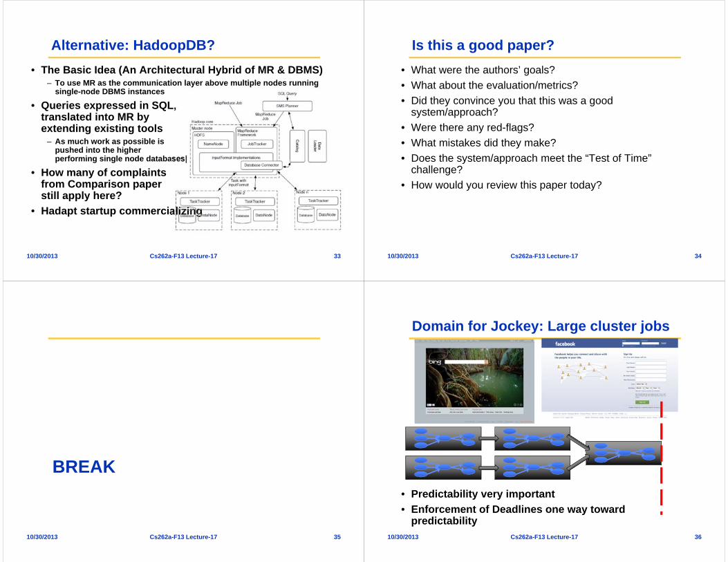
UDF Aggregation Task• Compute inlink count per document• SQL:
SELECT INTO Temp F(contents) FROM Documents;SELECT url, SUM(value) FROM Temp GROUP BY url;
Need a user-defined-function to parse HTML docs (C pgm using POSIX regex lib)
Both DBMS’s do not support UDF very well, requiring separate program using local disk and bulk loading of the DBMS – why was MR always forced to use Reduce to combine results?
• MR:– A standard MR program
10/30/2013 31Cs262a-F13 Lecture-17
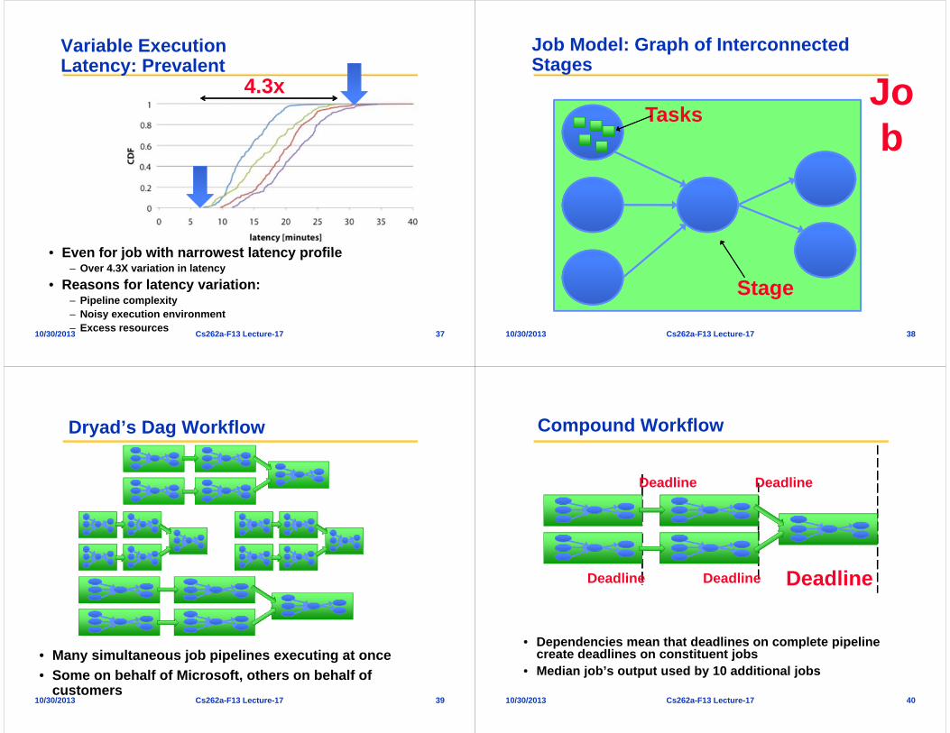
UDF Aggregation
• DBMS: lower – UDF time; upper – other query time• Hadoop: lower – query time; upper: combine all
results into one
10/30/2013 32Cs262a-F13 Lecture-17
Discussion• Throughput experiments?
• Parallel DBMSs are much more challenging than Hadoop to install and configure properly – DBMSs require professional DBAs to configure/tune
• Alternatives: Shark (Hive on Spark)– Eliminates Hadoop task start-up cost and answers queries with sub-
second latencies» 100 node system: 10 second till the first task starts, 25 seconds till all
nodes run tasks– Columnar memory store (multiple orders of magnitude faster than disk
• Compression: does not help in Hadoop?– An artifact of Hadoop’s Java-based implementation?
• Execution strategy (DBMS), failure model (Hadoop), ease of use (H/D)
• Other alternatives? Apache Hive, Impala (Cloudera) ,
10/30/2013 33Cs262a-F13 Lecture-17
Alternative: HadoopDB?• The Basic Idea (An Architectural Hybrid of MR & DBMS)
– To use MR as the communication layer above multiple nodes running single-node DBMS instances
• Queries expressed in SQL, translated into MR by extending existing tools
– As much work as possible is pushed into the higher performing single node databases|
• How many of complaintsfrom Comparison paperstill apply here?
• Hadapt startup commercializing
10/30/2013 34Cs262a-F13 Lecture-17
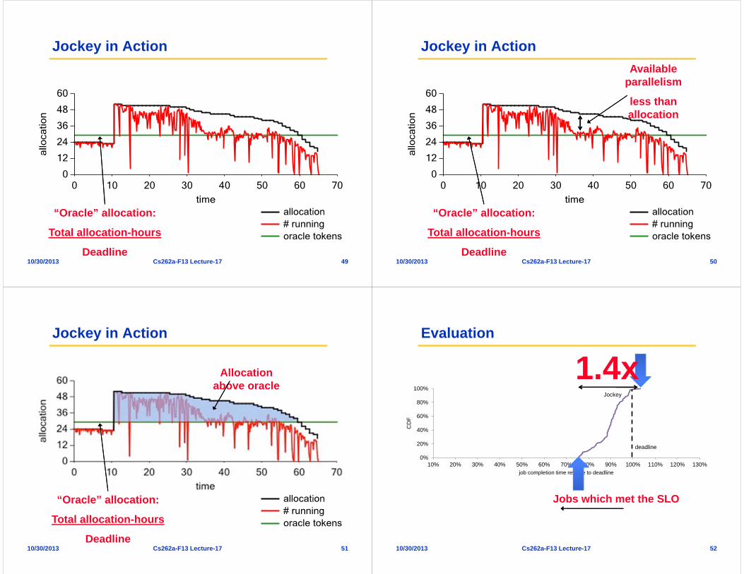
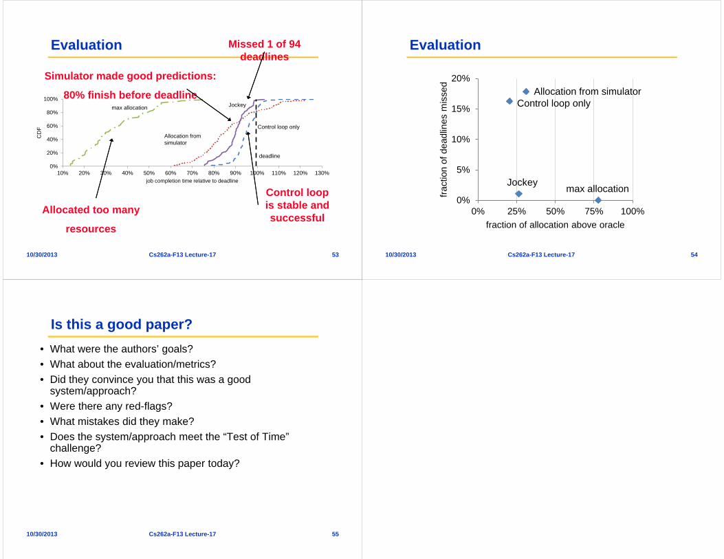
Is this a good paper?• What were the authors’ goals?• What about the evaluation/metrics?• Did they convince you that this was a good
system/approach?• Were there any red-flags?• What mistakes did they make?• Does the system/approach meet the “Test of Time”
challenge?• How would you review this paper today?
10/30/2013 35Cs262a-F13 Lecture-17
BREAK
10/30/2013 36Cs262a-F13 Lecture-17
Domain for Jockey: Large cluster jobs
• Predictability very important• Enforcement of Deadlines one way toward
predictability
10/30/2013 37Cs262a-F13 Lecture-17
Variable Execution Latency: Prevalent
• Even for job with narrowest latency profile– Over 4.3X variation in latency