HAL Id: tel-02950923 https://tel.archives-ouvertes.fr/tel-02950923 Submitted on 28 Sep 2020 HAL is a multi-disciplinary open access archive for the deposit and dissemination of sci- entific research documents, whether they are pub- lished or not. The documents may come from teaching and research institutions in France or abroad, or from public or private research centers. L’archive ouverte pluridisciplinaire HAL, est destinée au dépôt et à la diffusion de documents scientifiques de niveau recherche, publiés ou non, émanant des établissements d’enseignement et de recherche français ou étrangers, des laboratoires publics ou privés. Architecture for simultaneous multi-standard software defined radio receiver Sumit Kumar To cite this version: Sumit Kumar. Architecture for simultaneous multi-standard software defined radio receiver. Network- ing and Internet Architecture [cs.NI]. Sorbonne Université, 2019. English. NNT : 2019SORUS160. tel-02950923
Transcript
HAL Id: tel-02950923https://tel.archives-ouvertes.fr/tel-02950923
Submitted on 28 Sep 2020
HAL is a multi-disciplinary open accessarchive for the deposit and dissemination of sci-entific research documents, whether they are pub-lished or not. The documents may come fromteaching and research institutions in France orabroad, or from public or private research centers.
L’archive ouverte pluridisciplinaire HAL, estdestinée au dépôt et à la diffusion de documentsscientifiques de niveau recherche, publiés ou non,émanant des établissements d’enseignement et derecherche français ou étrangers, des laboratoirespublics ou privés.
Architecture for simultaneous multi-standard softwaredefined radio receiver
Sumit Kumar
To cite this version:Sumit Kumar. Architecture for simultaneous multi-standard software defined radio receiver. Network-ing and Internet Architecture [cs.NI]. Sorbonne Université, 2019. English. �NNT : 2019SORUS160�.�tel-02950923�
ARCHITECTURE FOR SIMULTANEOUS MULTI-STANDARDSOFTWARE DEFINED RADIO RECEIVER
SUMIT KUMAR
These dirigee par Prof. Florian Kaltenberger, Eurecom, France
Presentee et soutenue publiquement le 12 April 2019
Devant un jury compose de
Priv.-Doz. DI Dr. techn. Thomas Zemen RapporteurProf. Ghaya REKAYA-BEN OTHMAN RapporteurProf. Michel Terre JuryProf. Jerome Haerri JuryProf. Leonardo Cardoso JuryProf. George C. Alexandropoulos Jury
Acknowledgements
Foremost, I would like to express my sincere gratitude to my supervisor Prof. Florian Kaltenberger for thecontinuous support of my Ph.D. studies and related research, for his patience, motivation, flexibility, andimmense knowledge. His guidance helped me in all the time of research and writing of this thesis. His abilityto direct me towards alternative solutions when all the intuitive paths were blocked was precious. I couldnot have imagined having a better advisor and mentor for my Ph.D. study.
I would also like to sincerely thank my co-advisors from Siemens AG Corporate Technology, Munich, Dr.Alejandro Ramirez, and Dr. Bernhard Kloiber for their insightful critical comments which helped me im-prove my practical understanding of the subject matter.
I am deeply grateful to Kalyana Gopala, Elena Lukashova and Cedric Roux for their encouraging andstimulating discussions on the subject matter as well as day-to-day life matters.
Besides, I am very thankful to my friends Pramod Bacchav, Tsu Han Wangts, Roya Gholamipour, HaraldBayerlin, Rajeev Gangula, Konstantinos Alexandris, Christo Thomas and Leela Guddupudi for providingthe happy distraction to rest my mind outside of my research.
Last but not least, I am thankful to my family members for their continuous support, encouragementand sympathetic ear during my Ph.D.
1.1 Block diagram of a typical Software Defined Radio . . . . . . . . . . . . . . . . . . . . . . . . 121.2 WiFi Bluetooth Co-existence in a System on Chip (SOC). W1 and B1 are monolithic WiFi
and Bluetooth chips respectively on a single device. While W2 and B2 are WiFi and Bluetoothchips on separate devices. . . . . . . . . . . . . . . . . . . . . . . . . . . . . . . . . . . . . . . 14
2.1 A plausible schematic of a Simultaneous Multi-Standard SDR (SMS-SDR) . . . . . . . . . . 172.2 Due to finite ADC bitwidth/resolution, the weaker signal cannot span through the entire
dynamic range of the ADC in the presence of a stronger signal. This results in noise likerepresentation of the weaker signal after digitization. . . . . . . . . . . . . . . . . . . . . . . . 19
2.3 Frequency domain overlap of signals during CCI . . . . . . . . . . . . . . . . . . . . . . . . . 202.4 (a) Direct Conversion Receiver (b) Intermediate Frequency Receiver . . . . . . . . . . . . . . 202.5 Example flow diagram for mitigating CT-CCI from two heterogeneous wireless standards
4.9 PER of single antenna ZigBee receiver in the presence and absence of single antenna IEEE802.11g transmitter(transmit power -85 dBm). Even at −85 dBm, which is lower than theminimum receiver sensitivity of IEEE 802.11g, ZigBee observes severe PER degradation. . . . 36
4.12 Flow Chart of Interference Detection and LLR Scaling. LLR scaling using LNV (LNV-SC)to be performed only during interference. . . . . . . . . . . . . . . . . . . . . . . . . . . . . . 40
4.13 Performance of LNV-SC for IEEE 802.11g MCS 0 and 2 facing interference from single ZigBeechannel at −85 dBm. LNV-SC observes an average transmit power gain of 3.7 dB over Conv-SC for all the MCS. . . . . . . . . . . . . . . . . . . . . . . . . . . . . . . . . . . . . . . . . . 42
4.14 Performance of LNV-SC for IEEE 802.11g MCS 0 and 2 facing interference from two ZigBeechannels at −85 dBm. LNV-SC observes an average transmit power gain of 3 dB over Conv-SC for all the MCS. . . . . . . . . . . . . . . . . . . . . . . . . . . . . . . . . . . . . . . . . . 42
4.15 Performance of LNV-SC for IEEE 802.11g MCS 0 and 2 facing interference from four ZigBeechannels at −85 dBm. LNV-SC observes an average transmit power gain of 1.5 dB overConv-SC for all the MCS. . . . . . . . . . . . . . . . . . . . . . . . . . . . . . . . . . . . . . . 43
4
4.16 Noise Level Ratio: Ratio of the LNV of the interfered region to that of the region withoutinterference for fixed WiFi TXP -80 dBm. Even at low interference TxP of -100 dBm, theNLR is 6.5 dB which is sufficient to detect the presence of interference. . . . . . . . . . . . . . 43
4.17 Synchronization Error Rate (SER) of IEEE 802.11g MCS 2 and 4 after SIC of ZigBee (−80dBm). SER for both MCS is similar as the preamble of IEEE 802.11g is BPSK mobulatedregardless of the MCS . . . . . . . . . . . . . . . . . . . . . . . . . . . . . . . . . . . . . . . . 47
4.18 Packet Error Rate of IEEE 802.11g, MCS 2 after SIC of ZigBee (−80 dBm). Region overwhich SIC provides gain is highlighted in green rectangle. . . . . . . . . . . . . . . . . . . . . 47
4.19 Packet Error Rate of IEEE 802.11g, MCS 4 after SIC of ZigBee (−80 dBm). Region overwhich SIC provides gain is highlighted in green rectangle. . . . . . . . . . . . . . . . . . . . . 47
4.20 Single user frame format of IEEE 802.11ax . . . . . . . . . . . . . . . . . . . . . . . . . . . . 494.21 A block diagram of SC-FDMA . . . . . . . . . . . . . . . . . . . . . . . . . . . . . . . . . . . 494.22 Comparison of LNV-SC and Conv-SC in improving PER of IEEE 802.11ax MCS 0 facing
performs better than both MRC (with Conv-SC) and TIMO. ZigBee TxP −85 dBm . . . . . 574.28 Comparison of MRC(with Conv-SC), MLSC and TIMO for IEEE 802.11g MCS 2. MLSC
performs better than both MRC (with Conv-SC) and TIMO. ZigBee TxP −85 dBm . . . . . 574.29 Comparison of TIMO and DC-TIMO for IEEE 802.11g MCS 0. DC-TIMO benefits from the
additional diversity gains. ZigBee TxP −85 dBm . . . . . . . . . . . . . . . . . . . . . . . . . 584.30 PER of ZigBee after SIC of single channel IEEE 802.11g(MCS 0, TxP −85 dBm). . . . . . . 604.31 PER of ZigBee after SIC of single channel IEEE 802.11g (MCS 2, TxP −85 dBm). . . . . . 604.32 Schematic of SIC-MRC Receiver when IEEE 802.11g is the stronger signal and ZigBee is the
weaker signal . . . . . . . . . . . . . . . . . . . . . . . . . . . . . . . . . . . . . . . . . . . . . 624.33 PER comparison of ZigBee when SIC, SIC-MRC and Only MRC is applied, at IEEE 802.11g
MCS 0, TxP −85 dBm. SIC-MRC performs better than SIC. Plain MRC is also capable ofreducing PER in the event of interference. . . . . . . . . . . . . . . . . . . . . . . . . . . . . . 62
4.34 PER comparison of ZigBee when SIC, SIC-MRC and Only MRC is applied, at IEEE 802.11gMCS 2, TxP −85 dBm. SIC-MRC performs better than SIC. Plain MRC is also capable ofreducing PER in the event of interference. . . . . . . . . . . . . . . . . . . . . . . . . . . . . . 62
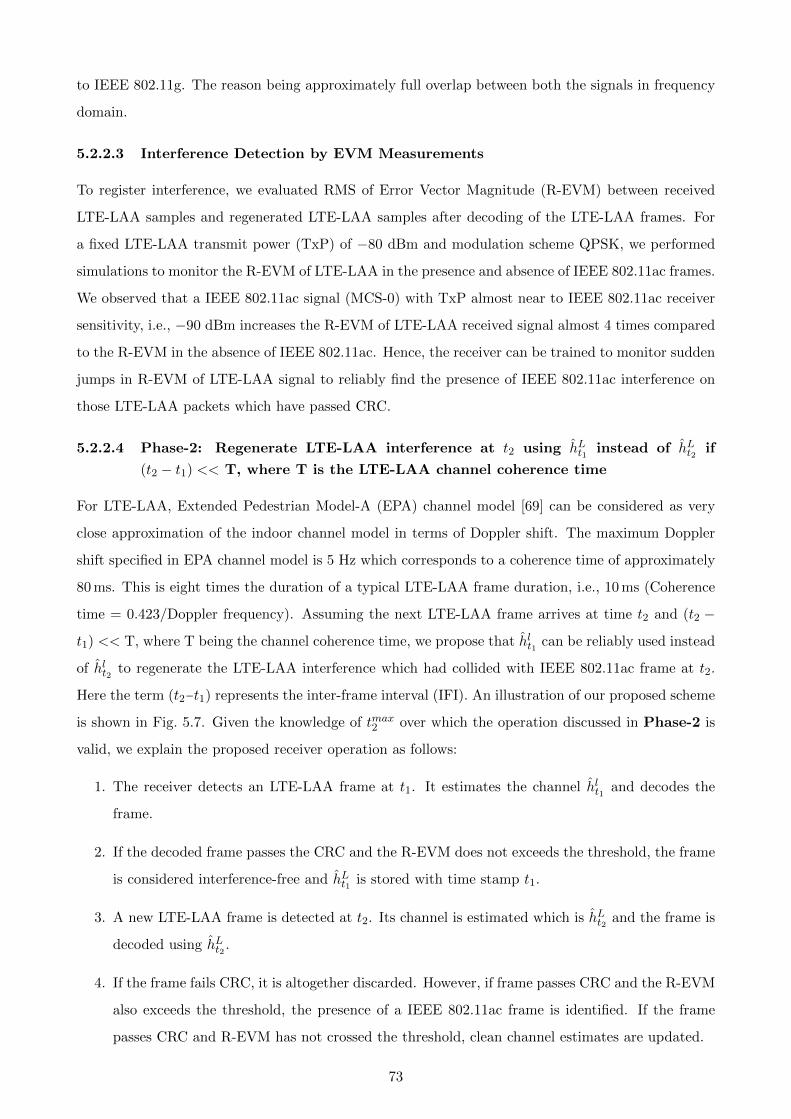
(L) and single antenna WiFi Plus LTE-LAA dual technology receiver (RX) . . . . . . . . . . 725.7 Proposed Scheme to Capture LTE-LAA Channel in the past and apply them in future. . . . . 725.8 Synchronization error of IEEE 802.11ac MCS 0: With and Without SIC, LTE-LAA −80
6.1 Decision tree for the parallel receivers attempting to decode signals S1 and S2 simultaneously.The result after parsing the decision trees is either decoding the signals or detecting theinterference. The figure continues to Fig. 6.2 . . . . . . . . . . . . . . . . . . . . . . . . . . . 85
detect narrowband interference in case the interferer is narrowband as in (a) or there is apartial overlap as in (c). However it fails when both signals have comparable bandwidths asin (b) . . . . . . . . . . . . . . . . . . . . . . . . . . . . . . . . . . . . . . . . . . . . . . . . . 88
6.4 (a) Decision tree to mitigate CT-CCI and recover wideband OFDM signal (b) Decision treeto mitigate CT-CCI and recover narrowband signal . . . . . . . . . . . . . . . . . . . . . . . . 90
6.5 (a) Decision tree to mitigate CT-CCI and recover OFDM signal in case of interference withanother OFDM signal (b) Decision tree to mitigate CT-CCI and recover Non-OFDM signalin case of interference with another Non-OFDM signal . . . . . . . . . . . . . . . . . . . . . . 90
6.6 (a) Decision tree to mitigate CT-CCI and recover wideband OFDM signal(b) Decision treeto mitigate CT-CCI and recover narrowband signal . . . . . . . . . . . . . . . . . . . . . . . . 91
6.7 (a) Decision tree to mitigate CT-CCI and recover OFDM signal facing interference fromanother OFDM signal (b) Decision tree to mitigate CT-CCI and recover a non-OFDM signalfacing interference from another non-OFDM signal . . . . . . . . . . . . . . . . . . . . . . . . 91
7.1 Soft Bit Maximal Ratio Combiner with LLR Scaling . . . . . . . . . . . . . . . . . . . . . . . 977.2 Over-the-air test set-Up: USRP B210, RF Cage and General Purpose CPU . . . . . . . . . . 987.3 Over-the-air Test Schematic corresponding to Section 7.4 . . . . . . . . . . . . . . . . . . . . 987.4 LNV-SC (proposed method) in the single interferer case leads to more IEEE 802.11g frames
passing CRC test compared to Conv-SC (conventional method) at a lower IEEE 802.11g TXP.This is observed for both the experimented interferer TXP . . . . . . . . . . . . . . . . . . . . 100
7.5 LNV-SC (proposed method) in the two interferer case also leads to more IEEE 802.11g framespassing CRC test compared to Conv-SC (conventional method) at a lower IEEE 802.11g TXP.This is observed for both the experimented interferer TXP . . . . . . . . . . . . . . . . . . . . 101
7.6 Branch-2 is partially covered with aluminum foil thus, receives lesser packets than Branch-1.In this case, SB-MLSC tracks Branch-1 which receives more packet than Branch-2. . . . . . . 101
7.7 Branch-1 is fully covered with aluminum foil and hence ceases to receive any packet. In thiscase, SB-MLSC tracks Branch-2 when Branch-1 is killed. . . . . . . . . . . . . . . . . . . . . . 102
7.9 GNU Radio Schematic For Double Receiver. The receiver is tuned to ZigBee channel-16 in2.4GHz ISM band. A double receiver operates by decoding all the branches simultaneously.This is contrast to selection combiner which selects one out of many available branches. . . . 103
7.10 Performance of ZigBee double receiver under several normalized receiver gain. As the gainincreases, both the antenna branches show similar performance. The experiment shows thatdiversity based reception show better performance when the system operate at the boundaryof noise limited region. . . . . . . . . . . . . . . . . . . . . . . . . . . . . . . . . . . . . . . . . 105
7.11 Functionality of a basic spectrum carving module for SMS-SDR. We have used spectrumcarving and channelizing synonymously in this thesis. . . . . . . . . . . . . . . . . . . . . . . 106
7.12 GUI of GNU Radio FreqXlating Filter Options. The block can be configured to performfrequency translation and decimation (if required) simultaneously. . . . . . . . . . . . . . . . 106
B.1 Soft bit metrics calculation in QPSK . . . . . . . . . . . . . . . . . . . . . . . . . . . . . . . . 117B.2 MRC vs SBMRC in the absence of interference. Both of them perform the same in the absence
of interference under the same channel conditions. . . . . . . . . . . . . . . . . . . . . . . . . 118
modems, the current focus is towards reconfigurability which will allow for rapid development and
deployment of future-proof designs. For example, the NVIDIA i500 will first ship with LTE Category
3 support; it will be upgraded via software to support LTE Category 4 with Carrier Aggregation.
In the current high-end smartphones and tablets, support for multiple standards in the single
device has become a de facto [75][65] practice. For example IEEE 802.11(a/b/g/n/ac): popularly
known as WiFi, IEEE 802.15.1: known as Bluetooth, IEEE 802.15 WPAN: known as RFID, Near
Field Communication (NFC), GPS, etc.
Let’s take the example of WiFi and Bluetooth operating in 2.4 GHz band. Currently, both the
standards are integrated monolithically on a single chip and share the antenna to save cost and space,
3Before the advent of FPGA, DSP (Digital Signal Processor) based SDR were used. DSPs are advantageous in termsof development infrastructure and developer familiarity. However, as the cost of FPGA has declined, a heterogeneouscombination of DSP and FPGA is frequently used.
13
WiFi (W1)
Bluetooth(B1)
Controlled Antenna Switch
WiFi(W2)
Bluetooth(B2)
UplinkDownlink
Fig. 1.2. WiFi Bluetooth Co-existence in a System on Chip (SOC). W1 and B1 are monolithic WiFi andBluetooth chips respectively on a single device. While W2 and B2 are WiFi and Bluetooth chips on separatedevices.
for example, Broadcom BCM43012[2], Cypress CYW43012[3]. Tasks in smartphone or tablets where
WiFi and Bluetooth are simultaneously active such as using Bluetooth headset during voice calling
over WiFi are very common and it ’appears’ that both WiFi and Bluetooth are transmitting/receiving
simultaneously; however they don’t, since they run in the same frequency band. Wifi transmits
using a contention-based mechanism CSMA/CA where before transmission it senses the medium and
transmits only if the medium is idle. On the other hand, Bluetooth performs frequency hopping
where it transmits briefly on a small chunk of spectrum, then instantly hops to a different frequency
to continue the transmission. Chip manufacturers design the transceivers using antenna control switch
in such a way that during transmissions only one of them; either WiFi or Bluetooth is active as shown
in Fig. 1.2. However, during the downlink traffic, especially during the initial stages of connection,
W2 is unaware of the traffic between B1 and B2 as there is no co-ordination between4 W2 and B2,
leading to collision, also known as Co-channel Interference (CCI). CCI is a known problem in wireless
communication caused by the hidden terminal and blind terminal [82][91].
But, what happens with the frames of WiFi and Bluetooth after they have interfered with each
other? If the Signal to Interference Plus Noise Ratio (SINR) is sufficient for both the signals after
interference, they can still be detected and decoded; if not, they are simply discarded. Thus, such
interference reduces the system throughput because of retransmissions. Several approaches have
been researched to address CCI mitigation, and most of them are based on isolation; temporal5 or
frequency6. However, any such isolation limits the system throughput again by putting a limitation
on the resources. Moreover, isolation based approaches require coordination between transmitters
of heterogeneous wireless standards which is not possible without modifying the standard. On the
other hand, if the SoC is capable of recovering the lost frame or correct the damaged frame after it is
detected, the throughput can be increased for both the involved signals. Besides, such a solution will
let both the wireless standards to transmit simultaneously without any contention for the channel.
In this thesis, we attempt to address the problem of CCI between heterogeneous wireless standards
operating in shared frequency bands, for example, IEEE 802.11g and IEEE 802.15.4 in the 2.4 GHz
ISM band, IEEE 802.11ac and LTE-LAA downlink in the 5 GHz ISM band, IEEE 802.11ax and LTE-
LAA(SC-FDMA) in the 5 GHz ISM band. ISM bands are characterized by a license-free operation;
hence, all the mentioned standards contend to use the channel without any centralized coordination
leading to frequent interference and throughput loss. Summary of the contributions in this thesis is
as follows:
4Same applies for the downlink transmission between B2 and B1 and the ongoing WiFi link5Assignment of different time slots for WiFi and Bluetooth6Assignment of different frequency bands to WiFi and Bluetooth
14
� Develop new physical layer signal processing methods to mitigate CCI as well as improvise
existing CCI mitigation methods which can detect and decode the heterogeneous signals which
are lost due to CCI. The signal processing methods will operate standalone on the receivers
without the requirement of any coordination from the transmitters.
� Test the developed methods for their applicability in general use cases by doing minimal cus-
tomizations. For example, wideband and narrowband signals, wideband and wideband signals,
etc.
� Develop Software Defined Radio (SDR) prototype for selected methods and verify the agreement
between simulations and results form over the air experiments. An SDR prototype enables rapid
deployment and customization of CCI methods for new use cases.
With the above contributions, we vision a Simultaneous Multi-Standard Software Defined Radio (SMS-
SDR). An SMS-SDR will be capable of decoding information from multiple heterogeneous wireless
standards simultaneously. The capability to receive multiple signals will be made possible by the CCI
mitigation techniques. Besides, an SMS-SDR can be customized for new wireless signals by updating
the software only. This will be in contrast to Simultaneous Multi-Standard Hardware Defined Radio
(SMS-HDR), which will possess the same capabilities as SMS-SDR; however, cannot be programmed
for new waveforms.
1.3 Organization of the thesis
� Chapter-2 starts with the discussion on theoretical research and field trials on various inter-
ference mitigation techniques. A significant part of our research focuses on developing cross-
technology interference mitigation methods. The focus is towards wireless standards in the
unmanaged networks in the ISM bands. State-of-the-art architectures of multi-standard SDR
platforms follow the discussion.
� Chapter-3 Discusses the details of proposed Simultaneous Multi-Standard SDR (SMS-SDR),
associated challenges and our proposed architecture to implement an SMS-SDR.
� Chapter-4 discusses CCI mitigation methods between wideband OFDM and narrowband signals.
We chose two typical and popular heterogeneous wireless standards operating in the 2.4 GHz
ISM band: IEEE 802.11g and ZigBee. We develop new methods and improvise known methods
for single and multi-antenna receivers. Next, we test some selective methods for another pair of
wideband OFDM and narrowband signal; IEEE 802.11ax and SC-FDMA to verify the general
applicability of the developed methods.
� Chapter-5 discusses CCI mitigation methods between wideband OFDM signals. We chose 20
MHz IEEE 802.11ac and LTE-LAA (LTE with Licensed Assisted Access) which will operate in
5 GHz ISM band and prone to CCI. Likewise chapter-4 we develop new methods and improvise
old methods for CCI mitigation in single and multi-antenna receivers.
� Chapter-6 collectively analyze all the signal processing methods developed in chapter-4 and 5.
We come up with a decision tree which states the chain of steps to be taken to detect and decode
Conference on Mobile Computing and Networking, 29 October-2 November 2018, New Delhi,
India
16
Chapter 2
Simultaneous Multi-Standard Software
Defined Radio
Our prime objective in this thesis is to develop the architecture for an SDR which is capable of
detecting and decoding multiple heterogeneous signals simultaneously. Our networks of interest are
random access networks where homogeneous/heterogeneous wireless standards operate on a shared
channel and compete among themselves to capture the transmission medium. In this chapter, we start
our discussion with the envisioned functionalities of the proposed Simultaneous Multi-Standard SDR.
We continue the discussion with the associated implementation challenges and finally, we present our
proposed architecture for an SMS-SDR.
2.1 SMS-SDR
The SMS-SDR we have envisioned will be capable of detecting and decoding multiple wireless signals
simultaneously. The signals could be homogeneous, i.e., belonging to the same standard as well as
heterogeneous, i.e., belonging to different standards. The architecture is in contrast to the current
state-of-the-art in SDR architecture which primarily focuses on reconfigurability and reusability of
the hardware and software signal processing blocks. A plausible and oversimplified illustration of
General Purpose Processor (GPP) based SMS-SDR is shown in Fig. 2.1. It consists of a single
Radio Frequency front-end (RF front-end) which is responsible for low noise amplification followed by
intermediate frequency translation, bandpass filtering and finally Analog to Digital Conversion. The
digitized signal after ADC is sent to FPGA where the signal is further down-converted and decimated
GPP
ChannelizationInterference MitigationRF
Front-end
FPGA
Standard-1: X1
Standard-2: X2
Standard-3: X3
X1
X2
X3
Detect & DecodeStandard-1
Detect & DecodeStandard-2
Detect & DecodeStandard-3
Fig. 2.1. A plausible schematic of a Simultaneous Multi-Standard SDR (SMS-SDR)
17
for sending the samples via USB or PCI port to the GPP.
We consider a random access network consisting on three different wireless standards: Standard-1,
Standard-2, and Standard-3 and the corresponding signals being X1, X2 and X3 respectively 1. The
mentioned standards share the medium of transmission, i.e., they operate on same frequency bands;
however, to avoid interference they follow Carrier Sense Multiple Access with Collision Avoidance
(CSMA/CA) [63]. CSMA/CA is based on energy detection of the radiated energy, and we will
see later in this chapter that under hidden terminal and blind terminal scenarios, CSMA/CA fails,
and transmitted frames from different nodes interfere with each other. In our work, we target such
scenarios of interference where CSMA/CA fails and multiple signals arrive at the receiver RF front-
end simultaneously. The other case, i.e., when CSMA/CA can avoid interference, is trivial to solve
as the signals will arrive at receiver one by one and can be detected and decoded.
Let’s assume a collision has happened, and as a consequence, X1 + X2 + X3 arrives at the RF
front-end through the antenna. The coarse operation of an SMS-SDR consist of the following steps:
� Step-1: Wideband sampling at the RF front end such that all the signals of interest are
captured. The sampled signal contains a mixture of X1, X2 and X3.
� Step-2: The sampled signal is sent to Channelizer in the GPP2. A Channelizer is used to
extract discrete communication channels located within a wideband signal. In our case, the
three signals have different bandwidths, so the Channelizer carves each of them out.
� Step-3: The next step is interference mitigation. As we see that our signals overlap each other
during concurrent operation, thus, before the signals are sent to their respective receivers, the
interference caused by other signals have to be cleaned. Successful operation of interference
mitigation yields detectable and decodable estimates X1, X2 and X3.
� Step-4: The estimates are further sent to their corresponding receiver chain for detection and
decoding.
The operation of SMS-SDR will be steered by many factors such as the number of antennas at the
receiver; received power levels, bandwidth, the modulation scheme of the signals; receiver mobility,
etc. The following sections discuss the challenges associated in implementing an SMS-SDR.
2.2 Challenges in Implementing SMS-SDR
The SMS-SDR will use a single RF front-end to capture multiple heterogeneous wireless signals.
Heterogeneous signals could be characterized by different modulation schemes, received power level,
sampling rates, bandwidths and center frequencies. Capturing signals with such wide disparity in their
physical layer characteristics using single RF front-end presents several challenges. A majority of such
challenges are related to the hardware begin used in an SDR such as Analog to Digital Converter
(ADC) and Channelizer. However, the impairment caused by hardware can be compensated to a large
extent in the GPP by applying signal processing software routines.
1For the sake of simplicity, we are omitting the channels and use whenever required2Channelizer can be implemented either in the FPGA or GPP
18
Stronger Signal
Weaker Signal
Am
plitu
de
Time
Am
plitu
de
Time
Am
plitu
de
Time
AGC ADC
Fig. 2.2. Due to finite ADC bitwidth/resolution, the weaker signal cannot span through the entire dynamicrange of the ADC in the presence of a stronger signal. This results in noise like representation of the weakersignal after digitization.
2.2.1 Finite ADC bit width
Different wireless standards arrive at the RF front-end with different received power levels. Any signal
arriving at the receiver first goes through Automatic Gain Control (AGC) which amplifies/reduces
the signal strength to span the entire range of ADC. In simpler words, AGC is performed so that
weak signal does not fall below the noise floor of ADC and the strong signal does not clip off and
saturates the ADC. If one of the many heterogeneous standards is significantly louder than others, a
higher resolution ADC will be required to capture the weaker signal. Reason being even after AGC,
the weaker signal may not be able to utilize the full resolution of the ADC. As shown in Fig. 2.2,
with less number of bits used to represent discrete samples of the weaker signal, in the worst case, the
weaker signal may appear as single bit noise after the digitization. Once the weaker signal becomes
noise like, it cannot be recovered with any signal processing technique. There could be three solutions
to this problem:
� Two separate RF front-ends with their AGCs configured for the stronger and weaker signals
respectively can be used to preserve the weaker signal; however, plugging as many RF front-ends
as the number of signals is not practical.
� Using very high-resolution ADC so that even with low gain by AGC, the weaker signal is
represented by as many bits as possible; however, the cost of AGC rises with the resolution.
� The weaker signal fades away in the quantization noise AGC is not able to sufficiently amplify
it because doing so will introduce clipping noise in the stronger signal. If the dynamic range of
ADC can be increased without inducing clipping noise, it may help the weaker signal to utilize a
few more bits. Ulbricht et al. in [93] proposed to apply diversity techniques using multiple ADC
to which improves the dynamic range of the ADC of a given bit width. According to them, using
multiple ADC of equal bit width can be used to overcome the inaccuracy and distortion caused
by using a single ADC of the same bit width. Cruz et al. in [31] proposed another parallel ADC
based solution which increases the dynamic range of the ADC by decreasing the clipping noise.
However, both the solutions require changes in the hardware and may not be of much interest
if Commercial Off the Shelf (COTS) hardware is being used for development.
within one OFDM symbol for IEEE 802.11g is shown in Fig. 4.1. Out of 64 subcarriers, 48 subcarriers
32
26 Subcarriers 26 Subcarriers
10 MHz 10 MHz
……………………… ………………………
Data Subcarriers
Pilot Subcarriers
Unused Subcarriers
Fig. 4.1. IEEE 802.11g Subcarrier Allocation
L-STF L-LTF L-SIG SERVICE bits Payload Pad bits Tail bits
Fig. 4.2. IEEE 802.11g Non-HT frame format
are used for data, 4 subcarriers as pilots and rest 11 subcarriers are unused to help isolate against
adjacent channel interference. Pilot subcarriers are used for phase correction in the OFDM data
symbols. Additionally, the DC subcarrier at the center is left unused to avoid DC leakage caused
by the usage of low-cost Direct conversion receivers. All the 48 data subcarriers are modulated with
the same modulation scheme. Supported modulation schemes in IEEE 802.11g are BPSK, QPSK,
16QAM, and 64QAM. Frame format of IEEE 802.11g is shown in Fig. 4.2. L-STF stands for Legacy
Short Training Frame and used for incoming frame detection, coarse frequency offset correction and
automatic gain control. L-LTF stands for Legacy Long Training Frame and used for symbol timing
offset correction, fine frequency offset correction, noise variance estimation, and channel estimation.
L-SIG is the Legacy SIGNAL field which contains information such as the modulation scheme used
for the payload, payload length, etc. L-SIG is always modulated using BPSK regardless of the
modulation used for payload. The payload contains the actual data to be transmitted. IEEE 802.11g
uses CSMA/CA for accessing the channel and avoiding collision.
4.1.2 ZigBee
ZigBee was conceived in 1998 and standardized in 2003 [41]. ZigBee is intended for low-throughput,
low-power, and low-cost applications. The 2.4 GHz ZigBee uses Offset Quadrature Phase Shift Keying
(O-QPSK) and Direct Sequence Spread Spectrum (DSSS) as the modulation scheme. In our work,
we have chosen 2.4 GHz ZigBee as IEEE 802.11g also operates in the same 2.4 GHz band and causes
CT-CCI. ZigBee uses IEEE 802.15.4 for its PHY and MAC while adds its propriety architecture for
the higher layers as illustrated in Fig. 4.3. Frame format of a typical ZigBee frame is shown in Fig. 4.4
The preamble consists of 8 zeros which are used for frame detection, Start of Frame Delimiter (SFD),
always set to 0X7A, is used to find the start of a packet, PHY header contains the length of the
payload which is the next field in the frame. Binary data coming from the application layers is first
spread using 16-ary orthogonal modulation using a set of orthogonal 32-bit chip sequence. Spreading
sequences yield multipath and ISI resistance. The resulting bit sequence is further modulated using
O-QPSK giving a baseband bandwidth of 2 MHz. Receiver sensitivity of ZigBee (Packet Error Rate
33
Application
API
Security
Network
MAC
PHY868MHz/ 915MHz/ 2.4Ghz
User
ZigBee Alliance
IEEE 802.15.4
Fig. 4.3. ZigBee OSI Architecture
Preamble Start of Frame Delimiter
PHY Header Payload
Fig. 4.4. ZigBee Frame Format
< 1%) is −85 dBm in 2.4 GHz ISM band. Likewise IEEE 802.11g, ZigBee also uses CSMA/CA for
accessing the channel and avoiding interference [102].
4.1.3 Interference Scenarios
The root of CT-CCI between IEEE 802.11g and ZigBee arises due to their frequency allocation in
the 2.4 GHz band as shown in Fig. 4.5 and Fig. 4.6. We see that IEEE 802.11g spans over 80 MHz
within which it has 14 channels, each 20 MHz wide; however at a given location and time only 3 of
them can operate in a non-overlapping manner. For example channel-1, 6 and 11. Channel-14 is not
commonly used (used only in Japan). In the same 2.4 GHz band ZigBee also spans over the entire 80
MHz band comprising of 16 non-overlapping channels each 2 MHz and frequency spacing of 5 MHz.
While all the IEEE 802.11g channels overlap with at least one or maximum four ZigBee channels,
ZigBee channel 4, 9, 15 and 16 are free from interference as shown in Fig. 4.7. Both IEEE 802.11g and
ZigBee use CSMA/CA for accessing the channel on the same frequency band. CSMA/CA is based on
energy detection where the transmitters sample the channel and compute the energy. If the energy
exceeds a predefined threshold, the channel is marked busy and the transmission time is deferred
according to an exponential backoff algorithm. The CSMA/CA mechanism works effectively even
if the wireless standards are different, i.e., IEEE 802.11g can defer its transmission when ZigBee is
transmitting on the same channel and vice-versa. However, in the situation of Hidden Terminal and
Blind Terminal as discussed in Section 3.2, CSMA/CA is ineffective. Especially the heterogeneity in
power level of IEEE 802.11g and ZigBee can readily cause hidden terminal problem [104]. Within an
IEEE 802.11g networks, the problem of the hidden and blind terminal is solved using the exchange
of RTS-CTS packets at the cost of reduced throughput[104];however there is no provision of such
mechanism between IEEE 802.11g and ZigBee. Going into the granular details of interference, for
IEEE 802.11g, the interference caused by ZigBee appears as frequency selective noise which is higher
on some of the subcarriers while lower on some of the subcarriers. For example, when a single ZigBee
channel overlaps with a single IEEE 802.11g channel, 20 MHz / 2 MHz, i.e., ≈ 7 subcarriers of IEEE
34
2.412 GHz 2.437 GHz 2.462 GHz 2.484 GHz
1 2 3 4 5 6 7 8 9 10 11 12 13 14
Channel Number
20 MHz 20 MHz 20 MHz 20 MHz
Rarely Used
Fig. 4.5. Frequency Allocation of IEEE 802.11g in 2.4 GHz band
1 2 3 4 5 6 7 8 9 10 11 12 13 14 15 16
2 MHz
F1 ……………………... FC …………………… F16
Channel Number
Fig. 4.6. Frequency Allocation of ZigBee in 2.4 GHz band
1 6 11 14
20 MHz
2 MHz
1 2 3 4 5 6 7 8 9 10 11 12 13 14 15 16
Interference
No Interference
Rarely Used
Interfered Subcarriers of IEEE 802.11g With single ZigBee Channel (Ch-7)
Non Interfered Subcarriers of IEEE 802.11g
Fig. 4.7. IEEE 802.11g and ZigBee overlap
802.11g (marked red in bottom of Fig. 4.7) get affected. To have an estimate of the performance
degradation of IEEE 802.11g caused by ZigBee, we performed a simulation of interference between
single antenna IEEE 802.11g receiver and interfered by fixed power single antenna ZigBee transmitter
(−85 dBm). 1. The Packet Error Rate (PER) is plotted in Fig. 4.8 which indicates severe degradation
of IEEE 802.11g PER for all the MCS which agree with the previous simulations and field trials. On
the other hand, the interference of IEEE 802.11g to ZigBee appears as frequency flat noise. To
assess the performance degradation of ZigBee caused by IEEE 802.11g, we performed simulations of
interference at a fixed IEEE 802.11g Transmit power of −85 dBm, MCS 0 and varying ZigBee power
with same simulation parameters as mentioned above. PER is plotted in Fig. 4.9 which again agree
with the previous studies.
In the event of CCI between IEEE 802.11g and ZigBee, an SMS-SDR is required to recover both
IEEE 802.11g and ZigBee from the collided packets it receives. In the coming sections, we develop
1Noise power = −100 dBm, 11 tap Rayleigh fading channel with exponentially decaying power delay profile for IEEE802.11g and single tap Rayleigh channel for ZigBee
35
-90 -85 -80 -75 -70 -65 -60 -55 -50
WiFi TXP dBm
10-4
10-3
10-2
10-1
100
WiF
i P
ER
MCS0
MCS2
MCS4
MCS6
No Interference MCS0
No Interference MCS2
No Interference MCS4
No Interference MCS6
10% PER Mark
Fig. 4.8. PER of single antenna WiFi receiver in the presence and absence of single antenna ZigBee transmit-ter(transmit power -85 dBm). For all IEEE 802.11g MCS, we observe severe PER degradation.
-120 -115 -110 -105 -100 -95 -90
ZigBee Transmit Power Level (dBm)
10 -3
10 -2
10 -1
10 0
Zig
Bee P
acket E
rror
Rate
No WiFi Interference
WiFi Interference of -85 dBm
Fig. 4.9. PER of single antenna ZigBee receiver in the presence and absence of single antenna IEEE 802.11gtransmitter(transmit power -85 dBm). Even at −85 dBm, which is lower than the minimum receiver sensitivityof IEEE 802.11g, ZigBee observes severe PER degradation.
36
physical layer signal processing methods to mitigate CCI for recovering both IEEE 802.11g and ZigBee
on single and multi-antenna receivers.
4.2 Mitigating CCI in Single Antenna IEEE 802.11g
Receiver Caused by ZigBee
In this section, we attempt to mitigate interference in single antenna IEEE 802.11g receiver caused
by up to 4 single antenna ZigBee transmitters. We chose Soft Decision IEEE 802.11g receiver instead
of Hard Decision Receiver because the former uses Soft Decision Viterbi Decoder (SDVD) which has
proven to be robust compared to Hard Decision Viterbi Decoder (HDVD) in an interference-limited
environment [60]. We start with a discussion on SDVD.
4.2.1 Soft Decision IEEE 802.11g Receiver and Noise Variance Estimation
After the incoming IEEE 802.11g frame has been detected and the frequency offset is corrected
(using L-STF and L-LTF), the next tasks are estimating the channel, performing equalization and
then decoding the data. The L-LTF symbol of the OFDM frame, as shown in Fig. 4.2 is used for
channel and noise variance estimation. L-LTF consists of two identical OFDM symbols. After frame
boundaries of the OFDM frame are detected (timing offset correction) and removal of cyclic prefix
of every OFDM symbol, a N (N = 64 for IEEE 802.11g) point FFT of the OFDM frame is taken to
obtain frequency domain samples which are written as:
Y (i, j) = X(i, j)H(i, j) + n(i, j), 1 ≤ i ≤ N, (4.1)
where Y (i, j), X(i, j) are complex samples representing received and sent symbols on the i-th subcar-
rier of the j-th OFDM symbol, respectively. Also, H(i, j) is the channel transfer function of the i-th
subcarrier for the j-th OFDM symbol. Term n(i, j) contains components from both thermal noise,
which is Gaussian and interference, which is not necessarily Gaussian. However, for this work, we
model both noise sources as Gaussian with zero mean and variance σ2 = {|n(i, j)|2}. To estimate σ2,
L-LTF is used and the conventional way [76] of doing it is to perform an average over noise variances
of all used subcarriers Usub (52 for IEEE 802.11g [46]) in the L-LTF as follows:
σ2 =1
2Usub
Usub∑i=1
|Y (i, 1)− Y (i, 2)|2, (4.2)
where Y (i, 1), Y (i, 2) are the complex samples corresponding to i-th subcarrier of the first and second
L-LTF symbols respectively. This σ2 is used as noise variance for all the subcarriers of the OFDM
data symbols following the L-LTF, i.e., SIGNAL and Payload field. The estimated noise variance
is used to compute the approx Log Likelihood Ratios (LLRs) on per subcarrier basis 2. The LLR
Λ(i, j, l) of the l-th bit corresponding to i-th subcarrier from j-th OFDM symbol is obtained as follows
[80, Eq-2]:
Λ(i, j, l) =
minz∈Zl
0
(|Y (i, j)−H(i, j)z|2
)σ2
−minz∈Zl
1
(|Y (i, j)−H(i, j)z|2
)σ2
(4.3)
2In practice, the LLRs are approximated for efficiency and the approx LLRs [96],[80] are used in SDVD. From thispoint, we use the term LLR and approx LLR interchangeably.
37
where Z(l)q = {z|bl(z) = q} and bl denotes the l-th bit in the gray mapping of z and σ2 is the
conventional noise variance estimate. We observe that the noise variance σ2 acts as a scaling factor
which scales the LLRs Λ(i, j, l) according to the extent of noise variance on that subcarrier. A higher
noise variance decreases the LLR while a smaller noise variance increases the LLR. We term the
method of scaling the LLRs as in (4.3) as Conventional LLR Scaling (Conv-SC). In the absence of
interference, the noise variance across the subcarriers is flat, i.e., AWGN. Thus, scaling all the LLRs
using same noise variance estimate, i.e., Conv-SC works correctly. But, this is not the case in the
presence of narrowband interference. Let’s denote the set of all IEEE 802.11g subcarriers affected by
ZigBee as Sinterf and the set of rest of the subcarriers as Snon-interf. The Sinterf may contain both pilot
and data subcarriers. In the event of CCI, the noise variance on Sinterf is higher compared to the
noise variance on Snon-interf. Being the average noise variance over entire Usub, σ2 does not provide
local noise variance (LNV)information across Sinterf. Thus, the local estimation of noise power over
Sinterf and Snon-interf is required in order to justify the scaling of Λ(i, j, l).
4.2.2 Log-Likelihood Ratio Scaling with Localized Noise Variance of Interfered
IEEE 802.11g Subcarriers (LNV-SC)
In this section, we discuss our work of [54] where we overcome the limitation of Conv-SC and propose
modification to estimate local noise variance (LNV) estimates in the presence of single and multi-
ple narrowband ZigBee interferers. Nonetheless, the method is equally applicable to any type of
narrowband signal interfering wideband OFDM signal.
4.2.3 Localized Noise Variance Estimation
We start with a generalized case of K single antenna uncorrelated narrowband interferers (K single
antenna ZigBee transmitters) and a single antenna IEEE 802.11g receiver. In our settings, Sk is the
set of IEEE 802.11g subcarriers affected by the k-th ZigBee interferer (k = 1, . . . ,K) and S0 is the
set of all the subcarriers unaffected by any of the k interferers such that S0 ∪ S1 ∪ .... ∪ SK = SWiFi,
whereSWiFi is the set of all IEEE 802.11g subcarriers. As the center frequencies of IEEE 802.11g and
ZigBee in the 2.4 GHz band are fixed and their bandwidths are predefined, the knowledge of sets Sk
and the set S0 can be obtained apriori. An exemplary illustration for the case of 4 ZigBee interferers,
centered at 2.430, 2.435, 2.440 and 2.445 GHz interfering a single IEEE 802.11g channel centered at
2.437 GHz is shown in Fig. 4.10. In this case S1 = {1 . . . 7} and S2 ={17 . . . 23}, S3 ={32 . . . 38},S4 ={48 . . . 52} 3, S0 = SWiFi−S1−S2−S3−S4. Thus, |S1| = |S2| = |S3| = |S4| = 7, |S0| = 24 and
|SWiFi| = Usub where |B| means the cardinality of the set B. For k = 0, 1, . . . ,K, we define the LNV
estimate as follows:
σ2Sk=
1
2|Sk|∑i∈Sk
|Y (i, 1)− Y (i, 2)|2. (4.4)
We further define an index vector as
[VSk
]i
=
1, i ∈ Sk0, i /∈ Sk
i = 1, 2, . . . , Usub. (4.5)
3The last ZigBee channel affects only 5 subcarriers within the used subcarriers. Rest two affect subcarriers, i.e., 53and 54 are unused
38
S1 S0a S2 S0b S3 S0c S4
S0 = S0a ⋃ S0b ⋃ S0c SWiFi
SWiFi = S1 ⋃ S0a ⋃ S2 ⋃ S0b ⋃ S3 ⋃ S0c ⋃ S4
Interfered Subcarriers
Non Interfered Subcarriers
Fig. 4.10. Set of interfered and interference-free WiFi Subcarriers facing interference by 4 Co-Channel ZigBeeInterferers
Fig. 4.11. LNV estimates corresponding to 4 ZigBee Interferers. Distinguish lobes appear at ZigBee centerfrequencies due to LNV estimation.
Using (4.4) and (4.5), we define a vector of noise variances over Usub as:
σ2 =
K∑k=0
VSkσ2Sk
, (4.6)
Corresponding to Fig. 4.10, the plot of vector of noise variances σ2 for 4 ZigBee interferers to a single
WiFi channel is shown in Fig. 4.11. In the same figure, we also plot the noise variance obtained
conventionally, i.e., σ2 shown by a flat black line as it is constant over the entire span of used
subcarriers. In contrast, the plot of LNV vector, i.e., σ2, produce distinguishably elevated lobes
centered on the corresponding ZigBee center frequencies. Such lobes give information about two
important things:
� The presence of interferers
� The excess noise variance induced by the interferers
Finally using (4.4), (4.5) and (4.6), we can modify (4.3) to obtain the scaled LLRs as
Λ(i, j, l) =
minz∈Zl
0
(|y(i, j)−H(i, j)z|2
)σi
2 −minz∈Zl
1
(|y(i, j)−H(i, j)z|2
)σi
2 (4.7)
39
Detect Interference
Interference Detected
Perform LLR Scaling with LNV
Current Frame Ended
Yes
No
Yes No
Fig. 4.12. Flow Chart of Interference Detection and LLR Scaling. LLR scaling using LNV (LNV-SC) to beperformed only during interference.
where σi2 is the i-th element of the vector σ2 and i = 1, 2, . . . , Usub. We term our method of LLR
scaling using LNV estimates as LNV-SC. The LLRs are further sent to SDVD for the rest of the
processing steps.
To initiate the process of LNV-SC, the IEEE 802.11g receiver needs to know the presence or
appearance of single or multiple ZigBee interferers. In the next section, we discuss our method of
interference detection [54] which is a by-product of the computation of LNV-SC.
4.2.4 Multiple Narrowband Interference Detection
From Fig. 4.11, it is observed that for K number of interferers, the vector of noise variances σ2
observes sharp and distinguish rise in magnitude over the regions where the narrowband signals are
present compared to the regions unaffected by narrowband signals. For a given IEEE 802.11g channel,
the overlapping ZigBee channels center frequencies are known a priori from the frequency allocation
also shown in Fig. 4.6. Thus the elevated portions in Fig. 4.11 give a coarse estimate of the presence of
the interferers. This knowledge is combined along with a threshold detector to pinpoint the interferers
as soon as they appear. In practice, the LNV is estimated at all the possible center frequencies of
the interferer. Upon detecting the presence of interferers, the corresponding LNV is used to scale the
LLRs. The entire operation of interference detection and LLR scaling is illustrated in Fig. 4.12.
Our proposed method of interference detection does not add any additional signal processing
complexity as it is a byproduct of LNV-SC. The key advantage of our approach is that lobes could be
obtained even at the shallow level of interference. However, the method is effective only when there
is an overlap between L-LTF of IEEE 802.11g and an ongoing ZigBee transmission as the method
uses L-LTF (duration 0.8 µs) to calculate σ2. This is a fair assumption as the typical frame lengths of
IEEE 802.11g (194 µs− 542 µs) are shorter than that of ZigBee (352 µs− 4256 µs) [62]. To detect the
appearance of ZigBee interference during an ongoing IEEE 802.11g transmission, i.e., when L-LTF is
not interfered, pilot subcarriers embedded under every OFDM data symbols of IEEE 802.11g could
be used however the estimation accuracy could be affected as there are only 4 pilots subcarriers within
48 data subcarriers.
40
Table 4.1: Simulation Parameters
Channel Model WiFi11 tap Rayleigh, Exponential Power Delayprofile, RMS Delay Spread 49 ns
Channel Model ZigBee 1 tap Rayleigh
Noise Power −100 dBm
IEEE 802.11g PSDU 1000 bytes
ZigBee PSDU 120 bytes
Sampling RateWiFi 20 MHz, ZigBee oversampled to 20MHz
Table 4.2: Transmit Power Gain(dB) of LNV-SC compared to Conv-SC
#of Interferers
WiFi MCS0 2 4 6
1 3.9 3.5 3.8 3.8
2 3 3 2.9 2.7
4 1.5 1.5 1.5 1.2
4.2.5 Simulations and Results
To validate our methods LNV-Sc and interference detection, we perform Monte Carlo simulations
using the standard compliant IEEE 802.11g and IEEE 802.15.4 libraries available in release 2017b
of MATLAB. We simulated the worst case scenario, i.e., when lack of CSMA/CA creates a 100%
chance of collision. The simulation parameters are mentioned in Table 4.1. For all the experiments,
we choose Transmit Power level (TxP) required to achieve 10% PER as our performance metric4. We
simulate the entire RF front-end which includes simulating the behavior of frame synchronization and
timing synchronization in the presence of interference.
4.2.5.1 Comparing LNV-SC and Conv-SC
To compare LNV-SC and Conv-SC, we simulate interference between single IEEE 802.11g channel
and up to 4 ZigBee channels. TxP of ZigBee channels are fixed to −85 dBm which is the minimum
TxP required(in 2.4 GHz band) to achieve 1% PER [41], while IEEE 802.11g TxP is varied to achieve
< 10% PER. We present results for IEEE 802.11g MCS 0 (BPSK) and MCS 2 (QPSK) in in Fig. 4.13
and Fig. 4.14 respectively. We observe that with LNV-SC, the 10% PER mark is reached at a
lower TxP compared to Conv-SC. We term the difference in TxP observed between LNV-SC and
Conv-SC as Transmit Power Gain(TPG) which is summarized in Table 4.2 for MCS 0, 2, 4 and 6.
From Table 4.2 we observe the following:
� As the number of ZigBee channels increases, TPG monotonically decreases because more IEEE
802.11g OFDM subcarriers get affected which decreases the difference between noise variance
estimates calculated using Conv-SC and LNV-SC.
� TPG is consistent throughout the MCS for a given number of interferers. This is due to the
fixed payload size of IEEE 802.11g (1000 bytes) which we used for simulations leading to an
equal number of LLRs getting affected in all the MCS.
4This performance metrics criterion is mentioned in [46, Sec-17.3.10.4].
41
-100 -95 -90 -85 -80 -75 -70 -65
IEEE 802.11g Transmit Power Level (dBm)
10 -1
10 0
IEE
E 8
02
.11
g P
acke
t E
rro
r R
ate
MCS 0 Conv-SC
MCS 0 LNV-SC
MCS 2 Conv-SC
MCS 2 LNV-SC
MCS 0 W/o Interf
MCS 2 W/o Interf
Fig. 4.13. Performance of LNV-SC for IEEE 802.11g MCS 0 and 2 facing interference from single ZigBeechannel at −85 dBm. LNV-SC observes an average transmit power gain of 3.7 dB over Conv-SC for all theMCS.
-100 -95 -90 -85 -80 -75 -70 -65
IEEE 802.11g Transmit Power Level (dBm)
10 -1
10 0
IEE
E 8
02
.11
g P
acke
t E
rro
r R
ate
MCS 0 Conv-SC
MCS 0 LNV-SC
MCS 2 Conv-SC
MCS 2 LNV-SC
MCS 0 W/o Interf
MCS 2 W/o Interf
Fig. 4.14. Performance of LNV-SC for IEEE 802.11g MCS 0 and 2 facing interference from two ZigBee channelsat −85 dBm. LNV-SC observes an average transmit power gain of 3 dB over Conv-SC for all the MCS.
42
-100 -95 -90 -85 -80 -75 -70 -65 -60
IEEE 802.11g Transmit Power Level (dBm)
10 -1
10 0IE
EE
802.1
1g P
acket E
rror
Rate
MCS 0 Conv-SC
MCS 0 LNV-SC
MCS 2 Conv-SC
MCS 2 LNV-SC
MCS 0 W/o Interf
MCS 2 W/o Interf
Fig. 4.15. Performance of LNV-SC for IEEE 802.11g MCS 0 and 2 facing interference from four ZigBee channelsat −85 dBm. LNV-SC observes an average transmit power gain of 1.5 dB over Conv-SC for all the MCS.
-100 -98 -96 -94 -92 -90 -88 -86 -84 -82 -80
ZigBee Interference dB
10 0
10 1
10 2
10 3
No
ise
Le
ve
l R
atio
dB Noise Level Ratio
6.5 dB
Fig. 4.16. Noise Level Ratio: Ratio of the LNV of the interfered region to that of the region without interferencefor fixed WiFi TXP -80 dBm. Even at low interference TxP of -100 dBm, the NLR is 6.5 dB which is sufficientto detect the presence of interference.
4.2.5.2 Interference Detection
To test our method of interference detection, we calculate the ratio of the LNV of the interfered region
to that of the region without interference for a fixed WiFi TxP (−80 dBm) and varying TxP of a single
ZigBee channel from −100 dBm to −80 dBm. We term this ratio as Noise Level Ratio (NLR). In the
geometrical representation, the level of NLR defines the height of lobes relative to the noise floor as
illustrated in Fig. 4.11. The more prominent the lobe is, the more accurate is its detection using a
threshold detector. From Fig. 4.16, we observe that even at low interference TxP (−100 dBm), the
NLR is 6.5 dB which is sufficient to detect the presence of interference.
4.2.6 Discussion
A positive TPG for LNV-SC indicates that for a given IEEE 802.11g TxP, LNV-SC can achieve
lesser PER compared to Conv-SC. Lesser PER means more packets could be recovered in the event of
interference with ZigBee which fulfills the motive of SMS-SDR. However, LNV-SC is only capable of
recovering the packets which have already been detected. In other words SINR of IEEE 802.11g has
43
to be sufficient enough to be detected at the receiver, i.e., Frame Synchronization. In addition, due
to interference, the timing offset estimation could also be affected leading to wrong output of FFT
operation. Thus, if frame synchronization and timing offset detection fails; unfortunately the frame
cannot be recovered with LNV-SC. Nonetheless, LNV-SC is very simple to implement in the existing
IEEE 802.11g receivers as well as any wireless standard which uses OFDM for their PHY.
The efficiency of the NLR based interference detection method will depend upon the threshold
which will vary from one setting to another; hence an initial training and calibration will be required.
Nonetheless, NLR based method to detect the interference is a by-product of LNV-SC, i.e., no addi-
tional signal processing is required. On the down side, NLR can detect only narrowband interferers.
For wideband interferers, other methods such as Error Vector Magnitude (EVM) between decoded
and regenerated samples of the stronger signal can be used [56].
4.2.7 Limitations of LLR Scaling based Methods for OFDM Systems
Although LNV-SC provides significant gain while recovering interfered IEEE 802.11g packets, follow-
ing two cases could be argued where LNV-SC could malfunction:
� Case-1: LNV-SC requires IEEE 802.11g to be strong enough so that at least the frame synchro-
nization is successful in the event of collision. L-STF, which form the very beginning of a IEEE
802.11g frame are responsible for frame synchronization. L-STF are BPSK modulated to have
robustness, nonetheless, a high powered nearby ZigBee transmitter can destroy the structure of
L-STF leaving the entire IEEE 802.11g frame non-detectable.
� Case-2: If ZigBee frame corrupts an IEEE 802.11g frame in such a manner that L-STF and L-
LTF are not interfered, but SIGNAL field and payload are affected. In such case, the interference
cannot not be detected as discussed in Section 4.2.4. In the absence of interference detection,
LNV-SC will not function.
In the next section, we discuss methods which overcome the limitations of LNV-SC.
4.2.8 Successive Interference Cancellation of ZigBee from IEEE 802.11g
Successive Interference Cancellation is a well known physical layer technique to recover a weaker signal
corrupted by a stronger signal [71]. Let sz[n] and sw[n] be the time domain ZigBee and IEEE 802.11g
signals respectively. In the event of collision, the composite signal r[n] can be written as:
r[n] = hw[n] ∗ sw[n] + hz[n] ∗ sz[n] + v[n] (4.8)
where hw and hz are time domain impulse responses of IEEE 802.11g and ZigBee channels respectively.
Term v[n] represents Gaussian distributed thermal noise samples with zero mean and variance σ2.
Note that since the sampling rates of IEEE 802.11g (20 MHz) and ZigBee (2 MHz) are different, an
appropriate resampling needs to be performed before realizing (4.8). Without loosing the generality,
lets consider IEEE 802.11g as our SOI, the Signal to Interference plus Noise Ratio (SINR) of IEEE
802.11g in the received signal r[n] is
SINRWF[n] =E{|hw[n] ∗ sw[n]|2
}E{|hz[n] ∗ sz[n]|2
}+ σ2
. (4.9)
44
With this SINRWF, the detection and decoding of a IEEE 802.11g frame depend on the strength of
the ZigBee interference. In order to increase SINRWF, SIC can be applied over r[n]. SIC is possible
when the receiver can decode the stronger signal and cancel its effect from the composite signal. By
performing SIC, the effective post-processing SINR of the weaker signal is likely to exceed the required
receiver sensitivity [71] of the weaker signal. A power difference of 5-20 dBm is required for an efficient
operation of SIC [101]. It is possible to have such power difference when a strong ZigBee transmitter
is located nearby the IEEE 802.11g receiver.
The process of SIC starts when a strong ZigBee signal is detected and decoded at the receiver.
During the process of decoding, the channel estimates of ZigBee are stored, and once the decoded
bits are available, the channel estimates are used to regenerate the ZigBee signal back. In the next
section we first, discuss the channel estimation process for a detected ZigBee frame.
4.2.9 Channel Estimation for ZigBee
ZigBee employs direct sequence spread spectrum (DSSS) that uses a digital spreading function rep-
resenting pseudorandom noise (PN) chip sequences [41], [83]. The radio encodes these chip sequences
using orthogonal quadrature phase shift keying (O-QPSK) and transmits them at 2 Mchips/s or 250
Kbps. Thus the duration of one bit is 1/250000 = 4us. Maximum delay spread in 2.4GHz is of the
order of nano seconds [94] which is significantly less than the bit period of ZigBee which is 4us. This
indicates that in most of the environments, a ZigBee signal will experience frequency flat fading, i.e,
single tap channel in the time domain. However, unlike IEEE 802.11g, ZigBee does not have pilots
to estimate the channel. Nonetheless, the preamble structure of ZigBee as shown in Fig. 4.4 provides
an intuitive way of doing so. As shown in Fig. 4.4, the ZigBee frame is preceded by a Preamble and
Start of Frame Delimiter (SFD), jointly called Synchronization Header (SHR). Preamble consists of
4 byte, all set to 0 and SFD is 1 byte long with the value set to 0X7A. SHR is used at the receiver to
detect the incoming ZigBee frame, i.e., frame synchronization pin point the frame boundary. We use
the known symbols corresponding to SHR to estimate the single tap ZigBee channel. Consider the
transmitted vector Sz
and received vector Yz
corresponding to the known SHR samples as follows:
Yz
= hz ∗ Sz + V , (4.10)
where hz is the single tap channel, V is the noise vector. Each of the vectors in (4.10) are NX1 dimen-
sional where N is the total number of samples corresponding to SHR. 5. The Maximum Likelihood
estimate of hz can be written as:
hz =(S
z)TY
z
(Sz)TS
z (4.11)
Method as in (4.11) can be used to estimate the ZigBee channel only when it is single tap; nonetheless,
as discussed, indoor channel for ZigBee in 2.4 GHz is mostly single tap. For multi-tap ZigBee channel,
the method discussed in [59] can be used. Once the channel of ZigBee is estimated, next, we regenerate
the estimate of time domain ZigBee signal as follows:
yzReg[n] = hz[n] ∗ sz[n]. (4.12)
5In practice, many samples of Preambles are lost before the frame is detected, hence, samples corresponding to theSFD can be used for estimating the channel; however, the sampling accuracy may be affected
45
Note that we use only those ZigBee frames for regeneration which have passed the CRC test. After
that SIC is performed by subtracting the regenerated signal from the received signal:
After SIC, the post processing SINR of weaker WiFi becomes:
SINRSICWF[n] =
E{|hw[n] ∗ sw[n]|2
}E{|(hz[n]−hz[n]) ∗ sz[n]|2
}+ σ2
. (4.14)
From (4.14), it can be observed that the more accurate is the channel estimate hz, the smaller is
the noise term E{|(hz−hz) ∗ sz|2}+ σ2 in the denominator and the higher is post processing SINR of
IEEE 802.11g. With this post processing SINR, it is possible to detect the IEEE 802.11g frames in
the residue signal, i.e., ySIC[n] by performing the frame synchronization routines.
4.2.10 Simulations and Results
To validate the performance of SIC, we perform Monte Carlo simulations using the standard compliant
IEEE 802.11g and IEEE 802.15.4 libraries available in release 2017b of MATLAB. Interference is
caused by a single channel single antenna ZigBee transmitter whose TxP is fixed to −60 dBm. We
performed simulations for IEEE 802.11g MCS 2 and 4. Simulation parameters are the same as
mentioned in Table 4.1. We log Packet Error Rate (PER) and Synchronization Error Rate (SER)
as our performance metric. We first plot the SER for IEEE 802.11g MCS 2 and 4 in Fig. 4.17. We
observe that high powered ZigBee severely affects the frame synchronization of IEEE 802.11g frames,
i.e., IEEE 802.11g frames not being detected at all. Although performing SIC provides advantage
over no SIC, the overall SER stays very high. We also observe that SER for both IEEE MCS 0 and 2
are almost the same. This is explained by the fact that regardless of the MCS of IEEE 802.11g, the
preambles (L-STF and L-LTF) are always modulated using BPSK. Next we plot the PER for IEEE
MCS 0 and 2 in Fig. 4.18 and Fig. 4.19 respectively. We observe the following from PER plots:
� Presence of high power ZigBee severely degrades the PER of IEEE 802.11g. The degradation is
caused by synchronization error as well as CRC error.
� Performing SIC provides advantage over not performing SIC. This is observed over a region of
SNR which is highlighted by green rectangle in both the plots.
� The gain observed due to SIC fades away as the MCS increases. This can be explained by the
fact that at higher MCS, i.e., higher QAM constellations, the SINR requirement is also high
which may not be obtained by SIC.
4.2.11 Discussion
SIC overcomes the limitations of LNV-SC and MLSC. Nonetheless LLR scaling can again be applied
over the weaker signal for possible improvement in PER. A distinguish advantage of SIC is the
capability of resynchronization of the weaker signal, i.e., frame detection of weaker signal which is
otherwise undetectable due to interference. Although, we experimented for single ZigBee channel,
but the method can be extended for the case of multiple ZigBee channels too. Another significant
advantage of SIC is that it can be used for signals which have comparable bandwidth, which is
46
-100 -95 -90 -85 -80 -75 -70
IEEE 802.11g TxP (dBm)
10 -1
10 0
SE
R o
f IE
EE
80
2.1
1g
Without SIC MCS-2
With SIC MCS-2
No Interference MCS-2
Without SIC MCS-4
With SIC MCS-4
No Interference MCS-4
Fig. 4.17. Synchronization Error Rate (SER) of IEEE 802.11g MCS 2 and 4 after SIC of ZigBee (−80 dBm).SER for both MCS is similar as the preamble of IEEE 802.11g is BPSK mobulated regardless of the MCS
-100 -95 -90 -85 -80 -75 -70 -65
IEEE 802.11g TxP (dBm)
10 -1
10 0
PE
R o
f IE
EE
80
2.1
1g
Without SIC
With SIC
No Interference
Fig. 4.18. Packet Error Rate of IEEE 802.11g, MCS 2 after SIC of ZigBee (−80 dBm). Region over which SICprovides gain is highlighted in green rectangle.
-100 -95 -90 -85 -80 -75 -70 -65 -60 -55
IEEE 802.11g TxP (dBm)
10 -1
10 0
PE
R o
f IE
EE
80
2.1
1g
Without SIC
With SIC
No Interference
Fig. 4.19. Packet Error Rate of IEEE 802.11g, MCS 4 after SIC of ZigBee (−80 dBm). Region over which SICprovides gain is highlighted in green rectangle.
47
in contrast to LLR scaling based methods. However the benefits of SIC fade away as the QAM
constellations gets dense. Also, the performance of SIC majorly depends on the accurate regeneration
of the stronger signal which in turn depends on the accuracy of channel estimates. In the event of
interference, channel estimates accuracy, even for the stronger signal, is affected. In next sections and
chapters, we propose methods to overcome these limitations of SIC.
4.3 Testing LNV-SC for its General Applicability
With the discussion of SIC, our development of interference mitigation methods for single antenna
wideband OFDM receivers is finished. Before we proceed to multi-antenna receivers, we briefly test
LNV-SC for its generalized applicability to other wireless signals. We choose IEEE 802.11ax [37], [23]
as the wideband OFDM signal and another signal which is based on SC-FDMA [43] as the narrowband
signal. We start with a discussion on physical layer of both the signals followed by implementation of
LNV-SC to recover wideband IEEE 802.11ax from narrowband SC-FDMA interference.
4.4 Physical Layer of 802.11ax and SC-FDMA
IEEE 802.11ax is the upcoming generation in the IEEE 802.11 family with a scheduled release in 2019
end. It is also known as WiFi-6 and can achieve throughput upto 10 Gbps. It comes under High
Efficiency (HE) category with major changes in its physical layer. It will be operational in both 2.4
GHz and 5 GHz unlicensed band. SC-FDMA is not a wireless standard but a physical layer used by
LTE for its uplink in order to get more power efficiency. With the proposals by 3GPP to let LTE
enter in the unlicensed bands, termed as LTE Licensed Assisted Access(LTE-LAA), the interference
between IEEE 802.11ax and LTE-LAA is inevitable. We start our discussion with the physical layer
of IEEE 802.11ax and SC-FDMA in brief.
4.4.1 Physical Layer of 802.11ax
We choose IEEE 802.11ax as it is a wideband OFDM signal having physical layer different from previ-
ous IEEE 802.11 wireless standards. In contrast to IEEE 802.11n and IEEE 802.11ac which primarily
focus on high throughputs, IEEE 802.11ax focuses on efficiency. Some of the major advancements in
IEEE 802.11ax include:
� 256 point FFT compared to 64 point FFT in IEEE 802.11a/g/n/ac. Higher FFT point gives
more number of subcarriers within the same bandwidth of 20 MHz.
� OFDMA support in both uplink and downlink to enable multiuser support.
� LTE type resource allocation enables QoS for various users and services.
� Support for higher QAM such as 1024. This enables the gigantic achievable throughput of up
to 10 Gbps.
� 4x larger OFDM symbol duration provides improved robustness to outdoor environment char-
Fig. 4.20. Single user frame format of IEEE 802.11ax
Symbol Mapping S/P
M Point FFT
Subcarrier Allocation
P Point FFT
Cyclic Prefix
InsertionP/S
Fig. 4.21. A block diagram of SC-FDMA
A typical frame format for IEEE 802.11ax single user is shown in Fig. 4.20. We can see that the frame
consists of Legacy IEEE 802.11 Preambles also. Among the HE preamble, the HE-STF training
field is used for timing synchronization while the HE-LTF is used for channel estimation, enabling
beamforming and MIMO spatial diversity. 256 point FFT in IEEE 802.11ax results in 256 subcarriers
with a spacing of 78.125 KHz. Out of total 256 subcarriers, 234 are used as data subcarriers, 8 are
used as pilot subcarriers, 3 subcarriers at the center are left as DC and 11 subcarriers are unused.
4.4.2 SC-FDMA
SC-FDMA is a modulation scheme used by LTE-LAA uplink as it provides significantly lower Peak to
Average Power Ratio (PAPR) compared to OFDM [72]. Likewise OFDM, SC-FDMA also produces
orthogonal subcarriers. A block diagram of SC-FDMA transmitter is shown in Fig. 4.21. The signif-
icant difference between SC-FDMA and OFDM transmitter is the insertion of an extra FFT block
before the IFFT block. Performing FFT before IFFT spreads the power evenly among subcarriers
reducing the PAPR [72]. In LTE-LAA, the resource allocation is performed in the units of Resource
Blocks where each resource block consists of 12 SC-FDMA subcarriers. By selecting appropriate num-
ber of resource blocks and sampling rates, the bandwidth of SC-FDMA can be varied. Section 4.4.2
shows the relation between number of resource blocks and the bandwidth in SC-FDMA signal.
4.4.3 Mitigating CCI in Single-antenna IEEE 802.11ax Receiver Caused by SC-
FDMA
We consider a scenario where a single antenna 20 MHz IEEE 802.11ax receiver is facing interference
from another single antenna SC-FDMA transmitter. We configure SC-FDMA for 3 MHz and 5 MHz
Table 4.3: SC-FDMA specifications used in LTE Uplink (20 MHz)
Channel Bandwidth (MHz) 20
Number of Resource Blocks 100
Number of Occupied Subcarriers 1200
IFFT/FFT (P in Fig. 4.21) 2048
Sample Rate (MHz) 30.72
49
Table 4.4: Simulation parameters for interference between IEEE 802.11ax and SC-FDMA
IEEE 802.11ax SC-FDMA
MCS 0 (BPSK) BPSK
Noise Power -100 dBm
Bandwidth (MHz) 20 3, 5
Sampling Rate (MHz) 20 3.84, 7.68
Channel Model TGax channel, Model-A Extended Pedestrian Channel Model-A
bandwidth by generating the waveform with 15 and 25 resource blocks respectively. This is the case
of interference between wideband OFDM signal and narrowband signal. Now we attempt to recover
IEEE 802.11ax signal by applying LNV-SC.
4.4.4 Applying LNV-SC to IEEE 802.11ax
LNV-SC requires computation of LNV estimates, however, the computation of LNV estimates in
a standard IEEE 802.11ax receiver posses some challenges. Out of total 256 subcarriers, only 8
subcarriers are used as pilot subcarriers for noise variance estimation. Thus they are not sufficient
for noise variance estimation per subcarrier as the spacing between the pilot subcarriers is large.
Although, L-LTF from the legacy preamble has 52 used subcarriers, 312.5 KHz wide each and IEEE
802.11ax payloads have 242 used subcarriers (pilot + data), 78.125 KHz wide each, both L-LTF
and payload occupy same bandwidth (in our case 20 MHz). Thus we propose to estimate the LNV
using L-LTF and map them over the payload subcarriers to span the entire used bandwidth of IEEE
802.11ax.
4.4.5 Simulations and Results
To validate the performance of LNV-SC over Conv-SC in recovering IEEE 802.11ax facing interference
from SC-FDMA signal, we created interference between single antenna single channel 20 MHz IEEE
802.11ax at MCS 0 (BPSK) and 3, 5 MHz SC-FDMA signals. Transmit power of SC-FDMA signal is
kept constant at −85 dBm. We perform Monte Carlo simulations using the standard compliant IEEE
802.11ax and SC-FDMA libraries available in release 2018a of MATLAB. We created the worst case
scenario as if there is not CSMA/CA making 100% chances of collision. Simulation parameters are
summarized in Section 4.4.4. We choose Transmit Power level (TxP) required to achieve 10% PER
as our performance metric for the experiments. PER plot for the case interference from 3 MHz and
5 MHz are shown in Fig. 4.22 and Fig. 4.23 respectively. From the plots we observe the following:
� Presence of SC-FDMA signal degrades the performance of IEEE 802.11ax. The degradation
increases with increase in the bandwidth of SC-FDMA signal as more number of subcarriers
of IEEE 802.11ax are affected. Quantitatively, since the subcarrier width of IEEE 802.11ax is
78.125 KHz, the number of affected subcarriers by 3 and 5 MHz SC-FDMA is approximately
39 and 64 respectively.
� Applying LNV-SC provides significant transmit power gain over Conv-SC. This is seen for both
3 MHz (6 dB of gain) and 5 MHz (5 dB of gain)SC-FDMA. As expected, the gain decreases
from 3 MHz to 5 MHz.
50
-100 -95 -90 -85 -80 -75 -70 -65
IEEE 802.11ax TxP (dBm)
10 -1
10 0P
ER
of
IEE
E 8
02
.11
ax
Conv-SC
LNV-Sc
No Interference
Fig. 4.22. Comparison of LNV-SC and Conv-SC in improving PER of IEEE 802.11ax MCS 0 facing interferencefrom 3 MHz SC-FDMA (−85 dBm) signal. LNV-SC performs better than Conv-SC
-100 -95 -90 -85 -80 -75 -70 -65
IEEE 802.11ax TxP (dBm)
10 -1
10 0
PE
R o
f IE
EE
80
2.1
1a
x
Conv-SC
LNV-Sc
No Interference
Fig. 4.23. Comparison of LNV-SC and Conv-SC in improving PER of IEEE 802.11ax MCS 0 facing interferencefrom 5 MHz SC-FDMA (−85 dBm) signal. LNV-SC performs better than Conv-SC
4.4.6 Discussion
In Section 4.2.2, through simulations, we show the effectiveness of LNV-SC in recovering wideband
OFDM IEEE 802.11g facing interference from narrowband ZigBee signals. In this section, we applied
the same method for a similar case of wideband OFDM and narrowband signals and observed similar
results where LNV-SC outperforming Conv-SC. These experiments prove the generality of LNV-SC.
4.5 Mitigating CCI in Multi-antenna IEEE 802.11g
Receiver Caused by ZigBee
Diversity is a well-known concept of combating the effects of multipath fading [90]. In particular,
we talk about spatial diversity which uses multiple antennas to extract uncorrelated fading signals.
By using omni-directional antennas and neglecting the effects of coupling between antennas, the
observations of signals on the multiple antennas would be uncorrelated if observed 0.38λ apart. The
underlying mechanism providing diversity gain is the decreasing probability of simultaneous deep
fades on all the antenna branches with an increasing number of antenna branches [33]. An additional
benefit of diversity is that likewise the desired signal, the interference also travels through different
paths, and if the path followed by interference corresponding to one antenna is in deep fade, it is
beneficial for the desired signal on that particular antenna! In this section, we attempt to leverage
this phenomena and extend our previous method LNV-SC for multi-antenna IEEE 802.11g receiver.
We consider the automated industries and smart homes where IEEE 802.11g and ZigBee nodes are
generously used; such environments are also characterized by rich multi-paths[19].
51
WiFi-Tx (X)
ZB-Tx (I)
WiFi-Rx
1
2
HX1
HX2
HI1
HI2
Fig. 4.24. Signal Model: Single Antenna IEEE 802.11g Transmitter, Single Antenna ZigBee Interferer and TwoAntenna IEEE 802.11g receiver
In the following, we discuss our work [55] which is a multi-antenna extension to LNV-SC. We
start our discussion with the popular diversity combining method Maximal Ratio Combiner followed
by legacy CCI mitigation method Optimal Combiner and state-of-the art CCI mitigation technique
Technology Independent MIMO (TIMO) [34]; but first we develop the multi-antenna signal model.
4.5.1 Multi-Antenna Signal Model
The signal model consists of a dual-antenna IEEE 802.11g receiver (WiFi-Rx), a single antenna IEEE
802.11g transmitter (WiFi-Tx), and a single antenna ZigBee transmitter (ZB-Tx) as illustrated in
Fig. 4.24. As IEEE 802.11g is our Signal of Interest (SOI), we assume that after collision, the IEEE
802.11g signal is strong enough to pass frame synchronization. After the correct timing offset detection
a 64 FFT is performed and the received signal vector Y on i-th subcarrier of j-th IEEE 802.11g OFDM
symbol with the desired IEEE 802.11g and interfering ZigBee samples X(i, j) and I(i, j) respectively
Channel estimation and all further signal processing is done in frequency domain, channels HX(i)
and HI(i) are assumed uncorrelated, while correlation ρX between channels of IEEE 802.11g HX1(i)
and HX2(i) and correlation ρI between channels of ZigBee HI1(i) and HI2(i) is non-zero. Note that
for the interference-free IEEE 802.11g subcarriers, ZigBee channels are not defined. Entries of the
noise vector n(i, j) contains components from both thermal noise, which is Gaussian and interference,
which is not necessarily Gaussian. However, for this work, we model both noise sources as Gaussian
as we did for single antenna case. Besides, the thermal noise variance is assumed to be constant
for a given OFDM frame while the noise induced by interferers vary from subcarrier to subcarrier.
Without loss of generality, we omit the subcarrier and OFDM symbol indexes (i, j) from notations of
the received vector Y, samples X and I and noise vector n and use them only when required.
52
4.5.2 Maximal Ratio Combiner and Optimal Combiner
Maximal Ratio Combiner(MRC) is one of the proven methods to increase the SNR of the signals in
a multi-antenna receiver [98]. In OFDM systems, MRC is performed on a per-subcarrier basis as
follows: [87]
YMRC = HHXY. (4.19)
Where YMRC is the complex sample after performing MRC, and HX denotes the estimated channel.
Although, MRC is capable of providing diversity gain the presence of uncorrelated multi-path fading
and array gain in case of correlated fading, the performance of MRC severely degrades in the presence
of CCI [98].
Optimal Combiner is a superset of MRC which, in the presence of colored noise (interference),
additionally computes Interference-plus-Noise (IPN) correlation matrix across all the receive antennas
and nullifies the interference [98],[87]. In a two antenna system, the optimally combined signal for
subcarriers experiencing interference (Sinterf) can be written as:
yOC = hHXφ−1RRy. (4.20)
Where φRR = E{[y1, y2
][y1, y2]
H}
(4.21)
is the IPN correlation matrix, and y1 and y2 are received signals on first and second WiFi-Rx antenna
respectively when only ZB-Tx transmits and WiFi-Tx is silent. For the interference-free subcarriers,
φRR = σ2I where I is M ×M identity matrix and σ2 is the noise variance. Thus, in the absence of
interference, OC acts as MRC [87, Eq-6.92]. The drawback of OC is that computation of φRR needs
to be performed for all the interfered subcarriers when only ZB-Tx transmits. Besides, φRR needs to
be updated with the period of coherence time of hI as it varies with channel fading rate. Both of
these conditions are difficult to meet in practice. Moreover, since φRR is a matrix of order M , the
computational complexity of matrix inversion grows with the number of antennas M .
4.5.3 Technology Independent MIMO
Technology Independent MIMO (TIMO) [34] applies Zero Forcing (ZF) receive beamforming using
two antennas to null the interference. Conventionally ZF receive beamforming requires exact channel
estimates of the interferer [35], [88], [14]. In contrast, TIMO uses the channel estimate ratio (β) of
the interferer, i.e., β = hI1/hI2 . Such property of TIMO makes it suitable for unmanaged networks
as obtaining the exact channel estimates of the interferer in unmanaged networks is impossible or
very costly due to the unknown structure of the interfering signals. The early work of TIMO ignores
noise [34, Eq-5,6] during computation of CER β. Hence, we refer to a recent work on TIMO in [105]
where authors consider the noise and use an MMSE estimator to compute CER β for the interfered
subcarriers as follows:
β =E{(IhI1 + n1)
(IhI2 + n2
)H}E{|y2|2}
. (4.22)
Considering an OFDM system, TIMO uses the β to null the interference on interfered subcarriers and
obtain the Signal Of Interest (SOI) as follows:
yinterfTIMO =y1−βy2
hX1−βhX2
. (4.23)
53
To compute SOI on the interference-free subcarriers, we first compute CER β for the interference-free
subcarriers by setting I = 0 in (4.22) and since, n1 and n2 are uncorrelated, it can be shown that
β = 0 for all the interference-free subcarriers. Hence, SOI for all the interference-free subcarriers
ynon-interfTIMO can be written as:
ynon-interfTIMO =y1
hX1
. (4.24)
Expression (4.24) is the well known Zero-Forcing Equalization (ZFE) over a single antenna [87, Sec-
7.3.1.1]. We observe that TIMO fails to exploit the diversity gain for all the interference-free sub-
carriers which potentially could be achieved using the already available two antennas of the TIMO
receiver. Additionally, CER β varies with the fading rate of hI and hence needs a continuous update
after every channel coherence period. Such requirements are difficult to guarantee in practice.
In the next sections, we discuss our work of [55] where we overcome the limitations of OC and
TIMO and develop methods to recover IEEE 802.11g on a multi-antenna receiver facing narrowband
ZigBee interference.
4.5.4 Maximum Ratio Combiner with Log-Likelihood Ratio Scaling (MLSC)
In our first method, we propose to perform MRC over signals from the receive antennas. This is
followed by scaling the obtained LLRs from MRC combined signal using a vector of Localized Noise
Variance (LNV) estimates aggregated over the receive antennas. We term our method as MLSC
(Maximum Ratio Combiner with Log-Likelihood Ratio SCaling) for the rest of the work. MLSC
receiver benefits from diversity gain as well as interference mitigation simultaneously. For a M antenna
IEEE 802.11g receiver, MLSC is performed on a per-subcarrier basis as follows:
1. Step-1: Combine the signals from M antenna branches according to MRC as in (4.19) and
obtain YMRC.
2. Step-2: Average the LNV vectors obtained from (4.6) over all the antennas as follows:
σAvg2 =
1
M
M∑m=1
σ2m. (4.25)
where σ2m is the noise variance vector corresponding to m-th antenna.
3. Step-3: Scale the LLR corresponding to the i-th subcarrier using σ2Avg(i), which is i-th element
of the vector σ2Avg, as follows:
Λ(i, l) =
minz∈Zl
0
(∣∣YMRC(i)−(|HX1(i)|2 + |HX2(i)|2)z∣∣2)
σ2Avg(i)
−minz∈Zl
1
(∣∣YMRC(i)−(|HX1(i)|2 + |HX2(i)|2)z∣∣2)
σ2Avg(i)
(4.26)
For a dual antenna IEEE 802.11g receiver, the schematic of MLSC is illustrated in Fig. 4.25.
54
Fig. 4.25. Schematic of Proposed MLSC for 2 Antenna WiFi Receiver
4.5.5 Diversity Combiner TIMO (DC-TIMO)
We have observed in Section 4.5.3 that TIMO does not exploit the potential diversity gain for all the
interference-free subcarriers in an OFDM system. We propose to solve this issue by performing MRC
on all the interference-free subcarriers. Our method is very simple and enables a TIMO receiver to
benefit from interference nulling on the interfered subcarriers as well as from diversity gain on the
interference-free subcarriers simultaneously. We term the proposed method as Diversity Combiner
TIMO (DC-TIMO). SOI with DC-TIMO for the interfered subcarriers yinterfDC-TIMO and the interference-
free subcarriers ynon-interfDC-TIMO is obtained as follows:
yinterfDC-TIMO =y1−βy2
hX1−βhX2
(4.27)
ynon-interfDC-TIMO = hH
Xy. (4.28)
4.5.6 Simulations and Results
To validate MLSC and DC-TIMO, we perform Monte Carlo simulations using the standard compliant
IEEE 802.11g and IEEE 802.15.4 libraries available in release 2017b of MATLAB. We simulate the
worst case scenario, i.e., when lack of CSMA/CA creates a 100% chance of collision. The simulation
parameters are mentioned in Table 4.1. For all the experiments, we choose Transmit Power level
(TxP) required to achieve 10% PER as our performance metric.
4.5.6.1 Comparing MLSC and OC
We simulate a dual antenna IEEE 802.11g receiver (WiFi-Rx) capable of performing OC and MLSC
simultaneously. The WiFi-Rx decodes packets received from a single antenna IEEE 802.11g trans-
mitter (WiFi-Tx) under interference from a single antenna ZigBee transmitter (ZB-Tx) as illustrated
in Fig. 4.24. Two different ZigBee TXP levels (−85 and −75) dBm are used. The correlation coef-
ficient ρX is fixed to 0.4 based on the measurements of [49]. Since, for both the OC and MRC, the
performance is agnostic of ρI [32], we fixed it to 0.1. In order to obtain φRR for OC as in (4.20), an
expectation was taken over approximately 80, 000 ZigBee samples collected from two receive antennas
of WiFi-Rx in order to guarantee the best performance of OC. PER for IEEE 802.11g MCS 0 is
plotted in Fig. 4.26. We also plot the PER of conventional MRC under the same setup. We observe
that for the mentioned ZigBee TxP (-75 dBm and -85 dBm), the performance of MLSC is quite close
to the of OC. The result can be explained by following two facts:
55
-100 -95 -90 -85 -80 -75 -70 -65
IEEE 802.11g Transmit Power Level (dBm)
10 -2
10 -1
10 0IE
EE
802.1
1g P
acket E
rror
Rate
MRC Conv-SC (ZigBee -75 dBm)
OC (ZigBee -75 dBm)
MLSC (ZigBee -75 dBm)
MRC Conv-SC (ZigBee -85 dBm)
OC (ZigBee -85 dBm)
MLSC (ZigBee -85 dBm)
Fig. 4.26. Comparison of MRC (with Conv-SC), OC and MLSC, for IEEE 802.11g MCS 0 and ZigBee TxP -85dBm
� OC nulls the interference on all the interfered OFDM subcarriers which effectively scales the
LLR obtained from all the interfered subcarriers. MLSC performs the same action by directly
scaling the LLRs obtained from all the interfered subcarriers in proportion to the LNV estimates.
� For the non-interfered subcarriers, both OC and MLSC boil down to MRC.
The advantage of MLSC over OC is that for a given IEEE 802.11g TxP, MLSC can achieve PER per-
formance very close to the OC but with a lower computational complexity and without the knowledge
of the statistics of the interferers.
4.5.6.2 Comparing MLSC and TIMO
We simulate the same scenario as in Section 4.5.6.1 with the difference that now the WiFi-Rx is able
to perform TIMO and MLSC simultaneously. IEEE 802.11g MCS 0 and 2 are simulated for a fixed
ZigBee TxP of −85 dBm. For TIMO, instead of estimating CER β as in [34, Eq-14], we directly
computed it from the channel realization of Zigbee to guarantee the best performance of TIMO. PER
is shown in Fig. 4.27 and Fig. 4.28 for IEEE 802.11g MCS 0 and 2 respectively. As a reference, we
also plot the PER when the two branches are combined using MRC and the corresponding LLRs are
scaled using Conv-SC. We observe that at the best, PER of TIMO is equivalent to MRC; however
the performance degrades as the IEEE 802.11g MCS goes high. On the other hand, MLSC provides
better PER compared to both MRC and TIMO. The key advantage of MLSC over TIMO is that
MLSC does not require the channel estimate ratio of the interferer.
4.5.6.3 Comparing TIMO and DC-TIMO
We simulate the same scenario as in Section 4.5.6.2 except now the WiFi-Rx is able to perform TIMO
and DC-TIMO simultaneously. IEEE 802.11g MCS 0 is simulated for a fixed ZigBee TxP of −85
dBm. CER β was computed directly from the channel realization of ZigBee to guarantee the best
performance of TIMO. PER is shown in Fig. 4.29. We observe that for a given TxP of IEEE 802.11g,
DC-TIMO achieves lower PER than normal TIMO which fails to benefit from the diversity gain.
Improvisation from TIMO to DC-TIMO is very simple, yet the gain is notable when a wideband
OFDM system gets interference by a narrowband signal.
56
-100 -95 -90 -85 -80 -75
IEEE 802.11g Transmit Power Level (dBm)
10 -1
10 0IE
EE
802.1
1g P
acket E
rror
Rate
MRC: Conv-SC
TIMO
MLSC
W/o Interference B-1: Conv-Sc
Fig. 4.27. Comparison of MRC(with Conv-SC), MLSC and TIMO for IEEE 802.11g MCS 0. MLSC performsbetter than both MRC (with Conv-SC) and TIMO. ZigBee TxP −85 dBm
-100 -95 -90 -85 -80 -75
IEEE 802.11g Transmit Power Level (dBm)
10 -1
10 0
IEE
E 8
02.1
1g P
acket E
rror
Rate
MRC: Conv-SC
TIMO
MLSC
W/o Interference B-1: Conv-Sc
Fig. 4.28. Comparison of MRC(with Conv-SC), MLSC and TIMO for IEEE 802.11g MCS 2. MLSC performsbetter than both MRC (with Conv-SC) and TIMO. ZigBee TxP −85 dBm
4.5.7 Discussion
� OC, although well known to null the CCI in a multi-antenna system, is practically not feasible
to implement due to computational complexity of IPN correlation matrix. In contrast, MLSC
achieves the same performance level as OC without knowing the statistics of the interferer. In
addition, practically it is possible to implement MLSC using SDR which is detailed in Chapter 7.
We use an implementation friendly method of MRC termed as Soft Bit Maximal Ratio Combiner
which is discussed in Appendix B.2.
� Likewise MLSC, TIMO is also practically feasible to implement in SDR as discussed by authors
in [34] and improves the PER in the event of interference. Obtaining the Channel Estimate
Ratio (CER) is practically possible because both IEEE 802.11g and ZigBee apply CSMA/CA
providing ample opportunities to measure the CER.
� In addition, DC-TIMO which is obtained by simple modifications to TIMO, shows notable per-
formance gain compared to TIMO. However, in the presence of an interference whose bandwidth
57
-100 -95 -90 -85 -80 -75
IEEE 802.11g Transmit Power Level (dBm)
10 -1
10 0IE
EE
802.1
1g P
acket E
rror
Rate
TIMO
DC-TIMO
No Interf
Fig. 4.29. Comparison of TIMO and DC-TIMO for IEEE 802.11g MCS 0. DC-TIMO benefits from theadditional diversity gains. ZigBee TxP −85 dBm
is comparable to the wideband OFDM, gain provided by DC-TIMO will be similar to TIMO.
In all the previous sections, our SOI was IEEE 802.11g. In the following sections, we make ZigBee as
our SOI and develop methods for its recovery while it faces CCI from IEEE 802.11g.
4.6 Mitigating CCI in Single Antenna ZigBee receiver caused by
IEEE 802.11g
Although ZigBee is inherently robust compared to IEEE 802.11g due to usage of spread spectrum
technique, the higher transmit power of IEEE 802.11g may result in severe PER degradation as seen
in previous works and shown in Fig. 4.9. In this section, we attempt to mitigate interference in a single
antenna ZigBee receiver caused by single antenna IEEE 802.11g transmitter. We chose Successive
Interference Cancellation (SIC) as our candidate method.
4.6.1 Successive Interference Cancellation of IEEE 802.11g from ZigBee
Referring (4.8) the Signal to Interference plus Noise Ratio (SINR) of ZigBee in the received signal
r[n] is:
SINRZB[n] =E{|hz[n] ∗ sz[n]|2
}E{|hw[n] ∗ sw[n]|2
}+ σ2
. (4.29)
With this SINRZB, the detection and decoding of a ZigBee frame depend on the strength of the IEEE
802.11g interference. In order to increase SINRZB, we apply SIC over r[n]. The post-processing SINR
of the weaker ZigBee signal is likely to exceed the required receiver sensitivity [71] of ZigBee receiver,
and thus could be decoded. Transmit power of IEEE 802.11g is 5-20 dBm [101] higher compared to
ZigBee which makes the application of SIC to recover weaker ZigBee from stronger IEEE 802.11g
favorable. The process of SIC starts when a strong IEEE 802.11g signal is detected and decoded
at the receiver. During the process of decoding, the channel estimates of IEEE 802.11g, which are
obtained from L-LTS, are stored. Once the decoded bits are available, the stored channel estimates
are used to regenerate IEEE 802.11g back. We explain the process as follows:
58
After the frame detection and N point (N = 64 for IEEE 802.11g) FFT of received samples, the
frequency domain complex sample Rw[k] on kth subcarrier of IEEE 802.11g is:
Rw[k] = Hw[k]Xw[k] +Hz[k]Iz[k] +N [k], (4.30)
whereXw[k], Iz[k] are frequency domain IEEE 802.11g and ZigBee symbols respectively. The elements
of Rw[k] corresponding to the pilot subcarriers are used to compute estimates Hw of the actual channel
Hw. Assuming that SINR of IEEE 802.11g is strong enough to allow the frame to pass the Cyclic
Redundancy Check (CRC), the next step is to regenerate the IEEE 802.11g frame for its sequential
cancellation from the time domain received signal r[n]. The regenerated frequency domain received
baseband IEEE 802.11g signal Y wReg[k] can be written as:
Y wReg[k] = Xw[k]Hw[k]. (4.31)
We use Xw and not the estimates because we regenerate only those IEEE 802.11g frames which have
passed CRC. We then convert Y wReg[k] into the time domain ywReg[n] by performing 64 point IFFT
which results in:
ywReg[n] = hw[n] ∗ sw[n]. (4.32)
Here hw[n] represents the time domain estimate of the IEEE 802.11g channel. After SIC of estimated
IEEE 802.11g interference the residue signal is now:
rSIC[n] = r[n]− ywReg[n] (4.33)
= hz[n] ∗ sz[n] + (hw[n]−hw[n]) ∗ sw[n] + v[n].
After SIC the effective SINR of weaker ZigBee becomes
SINRSICZB [n] =
E{|hz[n] ∗ sz[n]|2
}E{|(hw[n]−hw[n]) ∗ sw[n]|2
}+ σ2
. (4.34)
From (4.34), it can be observed that the more accurate the channel estimate hw, the smaller is the
noise term E{|(hw−hw) ∗ sw|2}+ σ2 in the denominator and the higher is post processing SINR of
ZigBee, i.e., SINRSICZB . Note that sampling rate of rSIC[n] is 20 MHz; hence before sending it to ZigBee
receiver it has to be downsampled at 2 MHz.
4.6.2 Simulations and Results
To validate performance of SIC in recovering ZigBee, we perform Monte Carlo simulations using the
standard compliant IEEE 802.11g and IEEE 802.15.4 libraries available in release 2017b of MATLAB.
Interference is caused by single channel IEEE 802.11g whose TxP is fixed to -85 dBm. We performed
simulations for IEEE 802.11g MCS 0 and 2 We use 10% PER mark as our performance metric.
Simulation parameters were same as mentioned in Table 4.1. Plots are shown in Fig. 4.30 and
Fig. 4.31. From the plots, we observe that SIC of IEEE 802.11g in the event of interference provides
approx 4 dB of gain compared to the case when SIC is not performed. The gain is consistent for all
the IEEE 802.11g MCS. Consistency with respect to MCS is obvious as the performance depends on
the post-processing SINR of ZigBee which is independent of the MCS of IEEE 802.11g.
59
-120 -115 -110 -105 -100 -95 -90
ZigBee Transmit Power Level (dBm)
10 -1
10 0
Zig
BeeP
acket E
rror
Rate
ZigBee W/o Interf
ZigBee with Interf
ZigBee after SIC of IEEE 802.11g
Fig. 4.30. PER of ZigBee after SIC of single channel IEEE 802.11g(MCS 0, TxP −85 dBm).
-120 -115 -110 -105 -100 -95 -90
ZigBee Transmit Power Level (dBm)
10 -1
10 0
Zig
Be
eP
acke
t E
rro
r R
ate
ZigBee W/o Interf
ZigBee with Interf
ZigBee after SIC of IEEE 802.11g
Fig. 4.31. PER of ZigBee after SIC of single channel IEEE 802.11g (MCS 2, TxP −85 dBm).
60
4.6.3 Discussion
SIC shows positive results during CT-CCI. In the coming sections, we will see the benefits of SIC
for other signals with different physical layers also. However, the performance of SIC is dependent
on how accurately the stronger signal has been regenerated which in turn depends on how accurate
the channel estimates of the stronger signal are. In the event of interference, the accuracy of channel
estimates get affected [47] resulting in reduction of the post-processing SINR of the weaker signal.
Additionally, as the number of ZigBee channels grows, post-processing SINR will further decrease. In
the next section, we present multi-antenna signal processing methods to overcome this limitation and
improve the performance of ZigBee SIC receiver through diversity gain.
4.7 Mitigating CCI in Multi-Antenna ZigBee receiver caused by
IEEE 802.11g
We have already seen the benefits of multi-antenna signal processing algorithms MLSC, TIMO and
DC-TIMO to mitigate CT-CCI. Also we have seen the benefits of SIC for single antenna ZigBee
receiver in Section 4.6.1. In this section, we develop SIC methods for multi-antenna ZigBee receivers.
4.7.1 SIC of IEEE 802.11g followed by MRC of ZigBee
SIC of IEEE 802.11g is effective in recovering the buried ZigBee signals as we have seen in Section 4.6.1.
However, the performance of SIC depends on the post-processing SINR of ZigBee which in turn
depends on channel estimation accuracy of the IEEE 802.11g signal. In the presence of ZigBee
interference, channel estimation accuracy of IEEE 802.11g is affected which increases the noise term
in the denominator of (4.34), i.e., E{|(hw[n]−hw[n]) ∗ sw[n]|2
}+ σ2. To reduce this noise, we propose
to perform MRC over ZigBee after the SIC of IEEE 802.11g. We start with the previous receiver
structure and extend it for a dual antenna receiver and perform SIC of IEEE 802.11g over both
the antenna branches. Following to that, we perform frame synchronization of ZigBee on both the
branches. Once frames are detected, MRC of the ZigBee signals is performed to reduce the noise
induced by inaccurate channel estimation of IEEE 802.11g. We term this receiver structure as SIC-
MRC for the rest of this work. A typical SIC-MRC receiver is shown in Fig. 4.32.
4.7.2 Simulations and Results
For the following experiments, we have the simulation settings, i.e. channel model for IEEE 802.11g
and ZigBee, payload lengths as in the previous simulations.
4.7.2.1 SIC-MRC
We simulate a dual antenna ZigBee receiver being interfered by a single antenna IEEE 802.11g trans-
mitter whose TxP level is fixed to −85 dBm. We use 10% PER mark as our performance metric.
In addition, we perform MRC over the two antenna branches of ZigBee without SIC. Results are
plotted for IEEE 802.11g MCS 0 and MCS 2 in Fig. 4.33 and Fig. 4.34 respectively. From the plots,
we first observe that SIC-MRC provides notable gain over plain SIC due to the fact that post-SIC
MRC reduces the residual noise induced by inaccurate channel estimation of the stronger signal. In
addition, we see that even plain MRC is capable of reducing the PER in the event of interference.
61
SIC of IEEE 802.11g
SIC of IEEE 802.11g
MRC of ZigBee ZigBee Decoder
Fig. 4.32. Schematic of SIC-MRC Receiver when IEEE 802.11g is the stronger signal and ZigBee is the weakersignal
.
-120 -115 -110 -105 -100 -95 -90
ZigBee Transmit Power Level (dBm)
10 -1
10 0
Zig
Be
eP
acke
t E
rro
r R
ate
ZigBee W/o Interf
ZigBee with Interf
ZigBee after SIC of IEEE 802.11g
SICMRC
MRC
Fig. 4.33. PER comparison of ZigBee when SIC, SIC-MRC and Only MRC is applied, at IEEE 802.11g MCS 0,TxP −85 dBm. SIC-MRC performs better than SIC. Plain MRC is also capable of reducing PER in the eventof interference.
-120 -115 -110 -105 -100 -95 -90
ZigBee Transmit Power Level (dBm)
10 -1
10 0
Zig
BeeP
acket E
rror
Rate
ZigBee W/o Interf
ZigBee with Interf
ZigBee after SIC of IEEE 802.11g
SICMRC
MRC
Fig. 4.34. PER comparison of ZigBee when SIC, SIC-MRC and Only MRC is applied, at IEEE 802.11g MCS 2,TxP −85 dBm. SIC-MRC performs better than SIC. Plain MRC is also capable of reducing PER in the eventof interference.
62
Table 4.5: Methods to detect interference
CT-CCI Detection Method Applies to
Detects thepresence orappearance ofinterferer
Limitations
Noise Level Ratio (NLR) be-tween LNV estimates of in-terfered and non-interferedwideband OFDM subcarri-ers
Wideband OFDM sig-nal facing interferencefrom single and multiplenarrowband signals
Already presentinterferer
Preamble ofwideband OFDMwhich is used toestimate LNVis required tointerfere withnarrowbandsignal
Error Vector Magnitude be-tween received signal and re-generated signal
Agnostic of the signaltype
Already presentas well as appear-ing interferer
Instantaneous de-tection of interfer-ence is not pos-sible without de-coding the datafirst
Finally, we observe that the benefits of SIC-MRC and MRC are agnostic with respect to the MCS of
IEEE 802.11g.
4.7.3 Discussions
In our previous discussion on the limitations of SIC in Section 4.6.3, we mentioned the excess noise
induced due to channel estimation inaccuracy of the stronger signal in the event of interference. SIC-
MRC proves itself effective in reducing such noise and increases the SINR of the weaker signal. This
results in reduced PER of the weaker signal. Although SIC-MRC is superior to SIC;however, it is a
complex operation and performing SIC on both antenna branches may further increase the complexity.
Interestingly we observed that a plain MRC could also provide gain in the presence of interference.
Hence depending on the available signal processing resources, a choice can be made among SIC-MRC
or plain MRC in a multi-antenna ZigBee receiver. In the next chapter, we continue our experiments
with SIC, MRC and SIC-MRC for the case of interference between two wideband OFDM signals.
4.8 Summary of the Methods
A summary of CT-CCI detection methods and CT-CCI mitigation methods is given in Table 4.5 and
LTE-LAA is the 3GPP standardized version of LTE-U (LTE in Unlicensed band). LTE-U did not have
the provision to listen before talk (LBT), and experimental evaluations showed severe performance
degradation of WiFi in the presence of LTE-U [20]. In LTE-LAA, 3GPP has made Listen Before
Talk (LBT) as a mandatory feature. LBT is similar to CSMA/CA where the transmitter has to sense
the channel before it transmits to check whether the channel is free or occupied. The LTE-LAA air
interface is based on OFDM for downlink and a Single-Carrier Frequency Division Multiple Access
(SC-FDMA) for the uplink. For 20 MHz of bandwidth, the sampling rate of LTE-LAA is 30.72
MHz, and it applies 2048 point FFT to generate the OFDM signal. The operating bandwidth is
approximately 20 MHz because only 1200 subcarriers out of 2048 subcarriers are used. After coding
and modulation, a transformed version of the complex-valued modulated signal termed as resource
element is mapped on to a time-frequency coordinate system called resource grid. It is a time-frequency
grid which is shown in Fig. 5.4. The resource grid has time on the x-axis and frequency on the y-axis.
In the time domain, LTE-LAA is structured as frame and subframes which is shown in Fig. 5.5.
Each frame is 10 ms in duration and consists of 10 subframes 1 ms each. Further, each sub-frame is
composed of two slots, 0.5 ms each. Finally, each slot consists of OFDM symbols, either seven or six
depending on whether a normal or an extended cyclic prefix has been used. In the frequency domain,
LTE-LAA is structured as resource blocks. Each resource block is made of 12 OFDM subcarriers,
hence, 180 KHz wide. 20 MHz LTE-LAA consists of 100 such resource blocks, hence occupies 18MHz
of used bandwidth out of 20 MHz usable bandwidth. Some of the subcarriers are left unused to both
68
Fig. 5.4. LTE-LAA Downlink Resource Grid
sides of the spectrum to relax the front-end filtering requirements. Channel estimation in LTE-LAA
is performed using Cell-Specific Reference Signals which are embedded in both time and frequency
domain inside a resource grid as shown by red dots in Fig. 5.4. For frame synchronization, timing
offset correction and frequency offset correction, LTE-LAA uses Primary Synchronization Sequence
(PSS) and Secondary Synchronization Sequence (SSS) [85].
5.1.3 Interference Scenarios
Although LTE-LAA uses LBT and IEEE 802.11ac uses CSMA/CA to access the channel, the situation
of the hidden terminal and blind terminal [104] persists in the case of LTE-LAA and IEEE 802.11ac
Fig. 5.5. Time Domain LTE-LAA
69
too. This is also indicated by previous simulations and field trials [103][100]. As there is no provision
of RTS-CTS (Request to send and Clear to send), packet exchange between IEEE 802.11ac and
LTE-LAA, the performance degradation could be severe.
There are two reasons why a frame is lost during a collision. Frame synchronization failure and
Cyclic Redundancy Check (CRC) failure. Frame synchronization is performed using preambles which
are very robust in nature as they use the lowest available MCS. IEEE 802.11ac uses BPSK and
LTE-LAA uses QPSK to modulate the preambles. At low power, if the collision happens, frame syn-
chronization fails and the frame is never detected. After a certain power level, frame synchronization
never fails, i.e., frame is always detected; however, now the frame is prone to CRC failures subjected
to the power on interference which also depends on the MCS used by the payload.
Knowing the mutual performance degradation of IEEE 802.11ac and LTE-LAA during simulta-
neous operation, in the next sections, we proceed towards developing signal processing methods to
mitigate the effects of interference and recover both LTE-LAA and IEEE 802.11ac. Our methods
reduce both frame synchronization and CRC failures in the event of interference.
5.2 Mitigating CCI in Single Antenna IEEE 802.11ac Receiver Caused
by LTE-LAA
In this section, we piggyback on the methods developed in Chapter 4 and use them for the case
of IEEE 802.11ac and LTE-LAA with IEEE 802.11ac as our Signal of Interest (SOI). Further we
improvise the SIC to increase its effectiveness for indoor deployments where the channel posses slow
fading characteristics.
5.2.1 SIC of LTE-LAA CCI from IEEE 802.11ac
In this section, without loosing the generality we assume LTE-LAA as the stronger signal and IEEE
802.11ac as the weaker signal. With the aforesaid assumption, we attempt to recover IEEE 802.11ac
by performing SIC of LTE-LAA frm the composite signal. Since, the theory of SIC is already estab-
lished in Chapter 4 and through simulations its effectiveness in mitigating CT-CCI between wideband
OFDM and narrowband signals is proved, we skip the theoretical details of SIC and proceed towards
implementation details for the particular case of IEEE 802.11ac and LTE-LAA.
Both IEEE 802.11ac and LTE-LAA standards have the provision of training signals for channel
estimation: Cell-Specific Reference Signals for LTE-LAA and VHT-LTF for IEEE 802.11ac. This
makes the prototyping a SIC-based receiver for both LTE-LAA and IEEE 802.11ac straightforward.
We assume that the LTE-LAA is strong enough such that after colliding with IEEE 802.11ac it
is still detected (frame synchronization) and frame boundaries are correctly detected (timing offset
detection). After 2048 point FFT, the samples are sent for channel estimation and decoding. Once the
70
frame passes CRC test, it is regenerated using the stored channel estimates. Next SIC is performed
and residue signal is resampled at 20 MHz and fed to IEEE 802.11ac receiver where it goes through
usual receiver processing starting with the frame synchronization routines. In Section 5.2.3 we perform
simulations to verify the performance of SIC.
In the next section, we improve SIC for low mobility conditions characterized by low Dopper
spread in the channels: a typical situation found in indoor environments.
5.2.2 SIC of LTE-LAA CCI from IEEE 802.11ac under Slow Fading Channel
(Indoor Environment)
From the discussion in Section 4.6.1, the post processing SINR of the weaker signal depends on the
accuracy of the channel of the stronger signal. When LTE-LAA is stronger than IEEE 802.11ac, the
post processing SINR of IEEE 802.11ac SINRSICW [n] can be written as:
SINRSICW [n] =
E{|hW [n] ∗ sW [n]|2
}E{|(hL[n]−hL[n]) ∗ sL[n]|2
}+ σ2
. (5.1)
where hW , hL are the time domain channels; sW , sL are the signals corresponding to IEEE 802.11ac
and LTE-LAA respectively. hL[n] is the estimated channel of LTE-LAA under interference and σ2
is the noise variance. Obtaining an accurate estimate of hL is difficult as LTE-LAA Cell-Specific
Reference Signals get corrupted by IEEE 802.11ac interference. Compared to the case of IEEE
802.11g and ZigBee, the CCI between IEEE 802.11ac and LTE-LAA more severely affects the channel
estimation as there is an almost full overlap of both the signals. Here we would like to emphasize
that up to a certain degree of the imperfect channel estimation; the LTE-LAA receiver is capable of
correct detection the data bits using Turbo decoders (likely at the price of an increased number of
turbo iterations). Nevertheless, the accuracy of channel estimates is significant for regeneration of
LTE-LAA interference to perform SIC.
5.2.2.1 Proposed Method
The most likely deployment of LTE-LAA will be through Small Cells [48]. In a small cell setting, access
points of both LTE-LAA and IEEE 802.11ac will be placed inside indoor environment as illustrated
in Fig. 5.63. We propose a method to perform SIC by using stored clean channel estimates of stronger
signals obtained during an interference-free period. Our approach leverages the high coherence time
of the indoor channel. Stating simply: if the channel coherence time is significantly larger than inter-
frame-interval (IFI)4, the channel estimates obtained in the past can be reused in the immediate
future, which is the basis of our proposal.
Let t1 be the time when there is no interference between IEEE 802.11ac and LTE-LAA frames and
3In the figure WiFi means IEEE 802.11ac4By IFI we mean the time of arrival of the subsequent frame
71
LTE LAA-Tx (L) WiFi-Tx (W)
Receiver (RX)
Downlink Uplink/DownlinkhL hW
LTE Macro Cell
Optical Fibre Link
Indoor Deployment
Fig. 5.6. An indoor deployment scenario of single antenna WiFi Tx (W), single antenna LTE-LAA Tx (L) andsingle antenna WiFi Plus LTE-LAA dual technology receiver (RX)
Fig. 5.7. Proposed Scheme to Capture LTE-LAA Channel in the past and apply them in future.
t2 be the time of interference (t2 > t1) as shown in Fig. 5.7. Also the LTE-LAA channel estimates at
time t1 and t2 be hLt1 , hLt2 respectively. We propose to regenerate the LTE-LAA interference occured at
time t2 using the interference-free LTE-LAA channel estimates hLt1 obtained at time t1 in the following
two phases:
5.2.2.2 Phase-1: Obtain clean LTE-LAA channel estimates at t1 when IEEE 802.11ac
frame is not being transmitted
Since IEEE 802.11ac uses CSMA/CA and LTE-LAA uses LBT, simultaneous transmission from both
of them is already minimized (except the hidden node case). Thus, there will be ample opportunities
for the receiver RX (in Fig. 5.6) for listening and decoding the ongoing LTE-LAA transmissions in
order to estimate the channel between LTE-LAA transmitter and the receiver. However, an obvious
question is how to confirm that the received LTE-LAA frame is interference free?
As discussed before, up to a certain degree of the imperfect channel estimation an LTE-LAA frame
can still pass CRC, thanks to the Turbo decoders. CRC failures cannot serve as a reliable indicator
of the presence or absence of the interferer because in the low SNR and no interference scenario, the
decoding might fail even if the receiver is provided with perfect channel estimates! Neither we can
use NLR based interference detection in Section 4.2.5.2 which is used to detect ZigBee’s interference
72
to IEEE 802.11g. The reason being approximately full overlap between both the signals in frequency
domain.
5.2.2.3 Interference Detection by EVM Measurements
To register interference, we evaluated RMS of Error Vector Magnitude (R-EVM) between received
LTE-LAA samples and regenerated LTE-LAA samples after decoding of the LTE-LAA frames. For
a fixed LTE-LAA transmit power (TxP) of −80 dBm and modulation scheme QPSK, we performed
simulations to monitor the R-EVM of LTE-LAA in the presence and absence of IEEE 802.11ac frames.
We observed that a IEEE 802.11ac signal (MCS-0) with TxP almost near to IEEE 802.11ac receiver
sensitivity, i.e., −90 dBm increases the R-EVM of LTE-LAA received signal almost 4 times compared
to the R-EVM in the absence of IEEE 802.11ac. Hence, the receiver can be trained to monitor sudden
jumps in R-EVM of LTE-LAA signal to reliably find the presence of IEEE 802.11ac interference on
those LTE-LAA packets which have passed CRC.
5.2.2.4 Phase-2: Regenerate LTE-LAA interference at t2 using hLt1 instead of hLt2 if
(t2 − t1) << T, where T is the LTE-LAA channel coherence time
For LTE-LAA, Extended Pedestrian Model-A (EPA) channel model [69] can be considered as very
close approximation of the indoor channel model in terms of Doppler shift. The maximum Doppler
shift specified in EPA channel model is 5 Hz which corresponds to a coherence time of approximately
80 ms. This is eight times the duration of a typical LTE-LAA frame duration, i.e., 10 ms (Coherence
time = 0.423/Doppler frequency). Assuming the next LTE-LAA frame arrives at time t2 and (t2 −
t1) << T, where T being the channel coherence time, we propose that hlt1 can be reliably used instead
of hlt2 to regenerate the LTE-LAA interference which had collided with IEEE 802.11ac frame at t2.
Here the term (t2−t1) represents the inter-frame interval (IFI). An illustration of our proposed scheme
is shown in Fig. 5.7. Given the knowledge of tmax2 over which the operation discussed in Phase-2 is
valid, we explain the proposed receiver operation as follows:
1. The receiver detects an LTE-LAA frame at t1. It estimates the channel hlt1 and decodes the
frame.
2. If the decoded frame passes the CRC and the R-EVM does not exceeds the threshold, the frame
is considered interference-free and hLt1 is stored with time stamp t1.
3. A new LTE-LAA frame is detected at t2. Its channel is estimated which is hLt2 and the frame is
decoded using hLt2 .
4. If the frame fails CRC, it is altogether discarded. However, if frame passes CRC and the R-EVM
also exceeds the threshold, the presence of a IEEE 802.11ac frame is identified. If the frame
passes CRC and R-EVM has not crossed the threshold, clean channel estimates are updated.
73
5. If t2 does not exceed tmax2 , hLt1 is used to regenerate the LTE-LAA signal instead of hLt2 , otherwise
hLt2 is used to regenerate the LTE-LAA signal.
6. Finally, the regenerated LTE-LAA interference is canceled from the composite signal and the
residue signal is downsampled to 20 MHz and sent for IEEE 802.11ac frame synchronization
and decoding.
5.2.3 Simulations and Results
To validate our method, i.e., SIC and SIC for slow fading channels, we perform simulations using the
standard compliant IEEE 802.11ac and LTE libraries available in MATLAB Release 2018a. In our
experiments, we use 20 MHz LTE bandwidth for the downlink and 20 MHz of 802.11ac bandwidth.
For proof of concept, we chose a fixed LTE-LAA TxP of −80 dBm and varied the IEEE 802.11ac
TxP. For each IEEE 802.11ac TxP, 100 frames were transmitted. We consider the worst-case scenario
as if there is no CSMA/CA or LBT making 100% chance of collision. The simulation parameters are
summarized in Table 5.1. As performance metrics we used total number of Synchronization errors
and Frame CRC errors.
Table 5.1: Simulation Parameters for LTE-LAA and IEEE 802.11ac Experiments
802.11ac LTE-LAA
Center Frequency 5 GHz 5 GHz
Bandwidth 20 MHz 20 MHz
Channel TGac Model-B EPA
Sampling Rate 20 MHz 30.72 MHz
Payload 500 Bytes 500 Bytes
Modulation and Coding MCS 0, 2, 4 QPSK
Noise Power −100 dBm −100 dBm
5.2.3.1 Experiment-1: Comparison between SIC with Instantaneous Channel Estimates
and No SIC
This experiment is performed to access the gain achieved by performing SIC in the case of CCI between
LTE-LAA and IEEE 802.11ac.We compare the performance between SIC with instantaneous channel
estimates and no SIC at all. We fixed the TxP of LTE-LAA at −80 dBm, modulation Scheme as
QPSK and SIC is performed using instantaneous channel estimates. For every TxP of IEEE 802.11ac,
we transmit 100 packets and log the number of received packets5 which pass CRC. Additionally, we
log all the frames which have been detected, i.e., synchronization is successful. First of all, we show
the synchronization error plot: with and without SIC. Note that regardless of the MCS used in IEEE
802.11ac, the preamble which is used for packet synchronization is always modulated using BPSK.
5We use the term frame and packet synonymously in this thesis.
74
-100 -95 -90 -85 -80 -75 -70 -65 -60
IEEE 802.11ac Transmit Power Level (dBm)
0
20
40
60
80
100
IEE
E 8
02
.11
ac S
yn
c F
ailu
re
With SIC
Without SIC
No Interference
Fig. 5.8. Synchronization error of IEEE 802.11ac MCS 0: With and Without SIC, LTE-LAA −80 dBm. Plotindicates that with SIC, the lost packets of IEEE 802.11ac caused by collision can be recovered.
Hence the synchronization error plot for MCS 0, 2 and 4 are same. We plot the results for MCS 0 in
Fig. 5.8 from which we observe that:
� IEEE 802.11ac synchronization failure significantly increases in the presence of LTE-LAA.
� Applying SIC notably reduces the synchronization failure. Considering a 40% sync failure rate,
applying SIC provides 15− 12 dB of transmit power gain compared to not applying SIC.
� Synchronization failure increases as the transmit power of IEEE 802.11ac reaches near the
transmit power (TxP) of LTE-LAA which is −80 dBm. This happens because as the TxP of
IEEE 802.11ac increases, LTE-LAA frames start getting corrupted (CRC test fails) and such
frames cannot be regenerated for SIC.
Next we show the frame error plots for IEEE 802.11ac MCS 0, 2 and 4 in Fig. 5.9, Fig. 5.10 and
Fig. 5.11 respectively. From the plots, we observe the following:
� Presence of LTE-LAA significantly degrades the performance of IEEE 802.11ac.
� Performing SIC of LTE-LAA helps in recovering IEEE 802.11ac packets which are lost due to
interference. However, the performance of SIC fades with an increase in the constellation size,
i.e., the MCS of the weaker signal (IEEE 802.11ac in this case). Because as the MCS increase,
the SINR requirement also increases which SIC fails to provide.
� We also observe that as the IEEE 802.11ac TxP reaches near to the TxP of LTE-LAA, i.e., −80
dB, the performance starts degrading. We have observed the same behavior previously in the
synchronization plots, and the same reasoning applies for the frame error case also.
75
-100 -95 -90 -85 -80 -75 -70 -65 -60
IEEE 802.11ac Transmit Power Level (dBm)
0
20
40
60
80
100
IEE
E 8
02
.11
ac P
acke
ts in
Err
or
With SIC
Without SIC
No Interference
Fig. 5.9. Frame Error for IEEE 802.11ac MCS 0: With and Without Using SIC, LTE-LAA TxP −80 dBm
-100 -95 -90 -85 -80 -75 -70 -65 -60 -55 -50
IEEE 802.11ac Transmit Power Level (dBm)
0
20
40
60
80
100
IEE
E 8
02
.11
ac P
acke
ts in
Err
or
With SIC
Without SIC
No Interference
Fig. 5.10. Frame Error for IEEE 802.11ac MCS 2: With and Without Using SIC, LTE-LAA TxP −80 dBm
-100 -90 -80 -70 -60 -50 -40
IEEE 802.11ac Transmit Power Level (dBm)
0
20
40
60
80
100
IEE
E 8
02
.11
ac P
acke
ts in
Err
or
With SIC
Without SIC
No SIC
Fig. 5.11. Frame Error for IEEE 802.11ac MCS 4: With and Without Using SIC, LTE-LAA TxP −80 dBm
76
-100 -95 -90 -85 -80 -75 -70 -65 -60
IEEE 802.11ac Transmit Power Level (dBm)
0
20
40
60
80
100
IEE
E 8
02
.11
ac S
yn
c F
ailu
re
SIC with Inst Channel
Without SIC
SIC with 2ms Old Channel
SIC with 10ms Old Channel
SIC with 20ms Old Channel
No Interference
Fig. 5.12. Synchronization error of IEEE 802.11ac MCS 0 at inter frame arrival times 2 ms, 10 ms and 20 ms,LTE-LAA −80 dBm
5.2.3.2 Experiment-2: Comparison between SIC with Instantaneous Channel Estimates
and SIC with Past Channel Estimates
With the same experimental settings as in Section 5.2.3.1, we simulate the interference between
LTE-LAA and IEEE 802.11ac with inter frame intervals of 2, 10 and 20ms. First we show the syn-
chronization error plot corresponding to IEEE 802.11ac MCS 0 in Fig. 5.12. Observing the plot, we
do not see any significant difference between SIC which uses old channel estimate taken 2ms before
the collision and the SIC which uses instantaneous channel estimates except for marginal gain till
−90 dBm. However, as we have seen in previous experiments, the performance of all types of SIC
degrades as TxP of IEEE 802.11ac reaches near the TxP of LTE-LAA which is −80 dBm.
Next, we show the frame error plots when we use channel estimates from the past to perform SIC
. Plots for IEEE 802.11ac MCS 0, 2 and 4 are shown in Fig. 5.13, Fig. 5.14 and Fig. 5.15 respectively.
We observe the following from the plots:
� Using old channel estimates notably reduces the frame errors, although cannot reduce the effect
of interference completely.
� If the collision happens within 2ms, SIC using the old channel estimates provides significant
advantage over SIC using instantaneous channel estimates.
� However, if the collision happens after 2ms, SIC using instantaneous channel estimates performs
better.
� Likewise inthe previous cases, we see performance degrades as IEEE 802.11ac TxP reaches near
the TxP of LTE-LAA which is −80 dBm.
77
-100 -95 -90 -85 -80 -75 -70 -65 -60 -55
IEEE 802.11ac Transmit Power Level (dBm)
0
20
40
60
80
100
IEE
E 8
02
.11
ac P
acke
ts in
Err
or
SIC with Inst Channel
Without SIC
SIC with 2ms Old Channel
SIC with 10ms Old Channel
SIC with 20ms Old Channel
No Interference
Fig. 5.13. Frame Error for IEEE 802.11ac MCS 0 at inter frame arrival times 2ms, 10ms and 20ms, LTE-LAA−80 dBm
-100 -95 -90 -85 -80 -75 -70 -65 -60 -55 -50
IEEE 802.11ac Transmit Power Level (dBm)
0
20
40
60
80
100
IEE
E 8
02
.11
ac P
acke
ts in
Err
or
SIC with Inst Channel
Without SIC
SIC with 2ms Old Channel
SIC with 10ms Old Channel
SIC with 20ms Old Channel
No Interference
Fig. 5.14. Frame Error for IEEE 802.11ac MCS 2 at inter frame arrival times 2ms, 10ms and 20ms, LTE-LAA−80 dBm
-100 -90 -80 -70 -60 -50 -40
IEEE 802.11ac Transmit Power Level (dBm)
0
20
40
60
80
100
IEE
E 8
02
.11
ac P
acke
ts in
Err
or
SIC with Inst Channel
Without SIC
SIC with 2ms Old Channel
SIC with 10ms Old Channel
SIC with 20ms Old Channel
No Interference
Fig. 5.15. Frame Error for IEEE 802.11ac MCS 4 at inter frame arrival times 2ms, 10ms and 20ms, LTE-LAA−80 dBm
78
5.2.4 Discussion
For a single antenna system, SIC is effective to mitigate the CCI. Not only it improves the perfor-
mance, but also it is capable of recovering lost frames. In other words, it acts as a re-synchronizing
receiver. Applying SIC using past channel estimates is beneficial inside an indoor environment which
is characterized by a slow fading channel, i.e., low Doppler; however the inter-frame arrival time
should be as low as 2ms. Besides, for any SIC to operate, the TxP of the weaker signal should be at
least 5− 10dB less than the stronger signal.
5.3 Mitigating Interference in Multi-Antenna IEEE 802.11ac Re-
ceiver Caused by LTE-LAA
5.3.1 SIC of LTE-LAA from IEEE 802.11ac followed by MRC
From Section 4.5.4 and Section 4.7.1 we have learned that SIC of stronger signal followed by MRC of
the weaker signal is capable of increasing the SINR of the weaker signal in a multi-antenna receiver. In
this section, we attempt to apply the same concept for a multi-antenna IEEE 802.11ac receiver facing
interference from LTE-LAA. Besides, to perform MRC, we apply implementation friendly Soft Bit
Maximal Ratio Combiner (SBMRC) as discussed in Appendix B.2. Since the MATLAB receiver for
Note that the operation of SBMRC followed by SIC does not have impact on the frame synchroniza-
tion, hence we we chose frame CRC failures as our performance metrics in this experiment.
5.3.2 Simulations and Results
In this experiment, we have the same simulation parameters as in Section 5.2.3.1 except now the re-
ceiver has two antennas. Antenna correlation was chosen to ’Low’ in the MIMOCorrelation parameter
of the EPA channel model in MATLAB. We compare following methods in this experiment:
1. SBMRC6 over the two antenna branches before SIC
2. SIC-SBMRC, i.e., SBMRC after SIC
3. SIC over single antenna with instantaneous channel estimates
4. SIC over single antenna with 2 ms old channel estimates
5. No SIC
Plots for IEEE 802.11ac MCS 0, 2 and 4 are shown in Fig. 5.16, Fig. 5.17 and Fig. 5.18 respectively.
From the plots we observe the following:
6We use MRC and SBMRC synonymously for this experiment
79
-100 -95 -90 -85 -80 -75 -70 -65 -60 -55
IEEE 802.11ac Transmit Power Level (dBm)
0
20
40
60
80
100
IEE
E 8
02
.11
ac P
acke
ts in
Err
or
SIC with Inst Channel
Without SIC
SIC with 2ms Old Channel
SBMRC afer SIC
SBMRC before SIC
No Interference
Fig. 5.16. Frame error for IEEE 802.11ac MCS 0: Performing SBMRC after SIC in a dual antenna receiver,LTE-LAA −80 dBm
-100 -95 -90 -85 -80 -75 -70 -65 -60 -55 -50
IEEE 802.11ac Transmit Power Level (dBm)
0
20
40
60
80
100
IEE
E 8
02
.11
ac P
acke
ts in
Err
or
SIC with Inst Channel
Without SIC
SIC with 2ms Old Channel
SBMRC afer SIC
SBMRC before SIC
No Interference
Fig. 5.17. Frame error for IEEE 802.11ac MCS 2: Performing SBMRC after SIC in a dual antenna receiver,LTE-LAA −80 dBm
-100 -90 -80 -70 -60 -50 -40
IEEE 802.11ac Transmit Power Level (dBm)
0
20
40
60
80
100
IEE
E 8
02
.11
ac P
acke
ts in
Err
or
SIC with Inst Channel
Without SIC
SIC with 2ms Old Channel
SBMRC afer SIC
SBMRC before SIC
No Interference
Fig. 5.18. Frame error for IEEE 802.11ac MCS 4: Performing SBMRC after SIC in a dual antenna receiver,LTE-LAA −80 dBm
80
� SIC-SBMRC outperforms SIC (both using old channels estimates and instantaneous channel
estimates)
� At MCS greater than 0 where the SIC, either using instantaneous channel estimates or the past
channel estimates, is unable to provide any performance gain; SIC-SBMRC provides notable
gain. Although the gain fades away as the MCS increases with the reason being post-processing
SINR after SIC-SBMRC not sufficient enough to decode the signals.
5.3.3 Discussion
SIC is an efficient method to mitigate CT-CCI, both in a single and multi-antenna receiver. SIC
followed by SBMRC provides increased post-processing SINR for the weaker signal. However, SIC
itself is a resource consuming process, and the computation power increases with the number of
antenna branches over which SIC has to be performed. Besides, SBMRC followed by SIC requires
LLR computation for all the antenna branches which could be resource consuming for higher MCS.
Thus, although SIC followed by SBMRC provides notable gain, a trade-off between system complexity
and performance has to be kept in mind while implementing the schemes on an SDR platform.
5.4 Summary of the Methods
We summarize the list of CT-CCI mitigation methods developed in this section in Table 5.2.
81
Tab
le5.
2:M
eth
od
sto
Mit
igate
CT
-CC
Ib
etw
een
two
wid
eban
dO
FD
Msi
gnals
Inte
rfere
nce
Mit
igati
on
Meth
od
Inte
rfere
nce
Sce-
nari
o
Nu
mb
er
of
Rx
Ante
nn
as
Recovers
Re-S
yn
cof
weaker
sign
al
Com
ments
Su
ccess
ive
Inte
rfere
nce
Can
-cellati
on
of
the
stro
nger
sig-
nal
(SIC
)
Ast
ron
gw
ideb
and
OF
DM
sign
al
gett
ing
inte
rfer
edby
anot
her
5−
20d
Bw
eak
wid
e-b
and
OF
DM
sign
al
1B
oth
the
sign
als
Yes
SIC
ofth
est
ron
ger
sign
alu
s-in
gold
chan
nel
est
imate
s
Sam
eas
abov
eb
ut
un
-d
erlo
wm
ob
ilit
yco
nd
i-ti
on
s1
Bot
hth
esi
gnal
sY
es
Su
itab
lefo
rlo
wm
ob
ilit
yen
vir
on
-m
ent
on
ly.
Inh
igh
mob
ilit
y,it
sb
ette
rto
use
inst
anta
neo
us
chan
-n
eles
tim
ate
s
SIC
of
the
stro
nger
the
sig-
nal
follow
ed
by
MR
Cof
the
weaker
sign
al
(SIC
-MR
C)
Ast
ron
gsi
gn
alge
ttin
gin
terf
ered
by
a5−
20d
Bw
eak
sign
al
und
erlo
wm
obil
ity
cond
itio
ns
2B
oth
the
sign
als
Yes
Per
form
ing
SIC
on
both
bra
nch
esfo
llow
edby
LL
Rco
mp
uta
tion
cou
ldb
eco
mp
lex,tr
ade-
off
cou
ldb
em
ake
bet
wee
neffi
cien
cyan
dav
ail
ab
lere
sou
rces
82
5.5 Publications
� Kumar, Sumit; Kaltenberger, Florian; Ramirez, Alejandro; Kloiber, Bernhard: A WiFi SIC
Receiver in the presence of LTE-LAA for Indoor Deployment. WCNC 2019, IEEE
Wireless Communications and Networking Conference,15-18 April 2019, Marrakech, Morocco
83
Chapter 6
Simultaneously Decoding
Heterogeneous Signals
In this chapter, we attempt to generalize the process of CT-CCI mitigation between any two given
heterogeneous wireless standards. We start by developing decision trees to determine the simultaneous
arrival of two heterogeneous wireless signals. Next, we design decision trees using the methods we
have developed in previous chapters to mitigate CT-CCI between the two heterogeneous signals based
on their physical layer characteristics.
6.1 Decision Tree: Interference Detection
In this section, we develop decision trees to detect the simultaneous arrival of two heterogeneous
wireless signals. We start with the case of two known and heterogeneous wireless signals S1 and
S2; both single antenna transmitters; whose physical layer characteristics, bandwidth, and frequency
allocations are known beforehand. The receiver; which is also a single antenna; has the capability
to decode both S1 and S2 simultaneously. Nonetheless, for both single antenna and multi-antenna
receivers, the decision tree will be the same to detect the simultaneous arrival. We are not expecting
any other collocated signal sharing its operating frequency band with S1 and S2. In other words,
we expect reception of either S1 or S2 or both. Furthermore, both S1 and S2 are operating in
interference limited region and not the noise-limited region.
A proposed decision tree, to be followed by the SMS-SDR to detect the simultaneous arrival
of two heterogeneous wireless signals is shown in Fig. 6.1 with its continuation in Fig. 6.2. The
receiver consists of two parallel receivers R S1 and R S2 responsible to detect and decode S1 and S2
respectively. During their course of operation, the receivers go through several states. The states of
R S1 are visible to R S2 and vice versa. The decision tree is valid for any two heterogeneous signals S1
and S2 which are fully or partially overlapping each other in the frequency domain, irrespective of their
physical layer characteristics. The very first step to receive S1 and S2 simultaneously is to perform
84
Start Detecting S2
End
S2 Detected
Detect Interference (S1)
Interference Detected
State: B1
State: B2
State: B3
State: B4
Decode S2 Attempt to Mitigate
Interference and Decode S2
End
No
Yes
Yes
No
Start Detecting S1
End
S1 Detected
Detect Interference (S2)
Interference Detected
State: A1
State: A3
State: A4
Decode S1 Attempt to Mitigate
Interference and Decode S1
End
No
Yes
Yes
No
State: A40 State: A30 State: B40State: B30
State: A2C D
R_S1 R_S2
Message Transfer
Decoding of S1 complete
Decoding of S1 complete after mitigating the effects of
interference from S2
Decoding of S2 complete
Decoding of S2 complete after mitigating the effects of
interference from S1
Fig. 6.1. Decision tree for the parallel receivers attempting to decode signals S1 and S2 simultaneously. Theresult after parsing the decision trees is either decoding the signals or detecting the interference. The figurecontinues to Fig. 6.2
No
End
C
Has R_S2 passed
through State: B3
Yes
D
Has R_S2 passed
through State: B1 and B2
YesEnd
No
State: A10
SIC of S2
Is S2 stronger than S1
Yes
End
No
End
No
End
Has R_S1 passed
through State: A3
Yes
Has R_S1 passed
through State: A1 and A2
YesEnd
No
State: B10
SIC of S1
Is S1 stronger than S2
Yes
End
No
End
Message Transfer
State: A100
State: A1000
State: A1001
State: B100
State: B1000
State: B1001
Neither S1 nor S2 has
been transmitted
S1 has not been
transmitted
Decoding of S1 not possible
Probable decoding of S1
Neither S1 nor S2 has
been transmitted
S2 has not been
transmitted
Decoding of S2 not possible
Probable decoding of S2
Fig. 6.2. Continuation of Fig. 6.1
85
channelization as discussed in Section 2.2.2; because in the beginning, the receiver does not know if
S1 and S2 have arrived simultaneously, i.e., interference has occurred; and thus receiver attempts
to decode both the signals S1 and S2. Without losing the generality, let us discuss the operational
details of R S1; nonetheless, the discussion is valid for R S2. There could be the following three
cases:
� Case-1: S1 is detected and S2 is not detected
In this case, the operation is straightforward. S1 is decoded and in the process of decoding S1,
an attempt is also made to detect the presence of S2, which could have been left undetectable
due to collision with S1. Refer Section 6.1.1 and Table 4.5 for a summary of the interference
detection methods. If S1 is detected, R S1 attempts to mitigate the effect of interference and
decode S1. In this case, the states R S1 goes through are: A1 → A2 → A3 → A30. In the
other case R S1 simple decodes S1 and terminates the operation. In this case, the states R S1
goes through are: A1 → A2 → A4 → A40.
� Case-2: S1 is not detected and S2 is detected
This could happen due to two reasons: Either S1 is not transmitted at all or S1 is undetectable
due to interference of S2. To find that, R S1 attempts to look further. During the decoding of
S2, R S2 could detect the presence of S1 (if S1 was transmitted at all) and pass through the
state B3. Thus R S1 first looks if R S2 has passed through B3.
– If R S2 has not passed through B3, that means S1 has not been transmitted or have been
left completely undetectable due to interference of S2. At this point R S1 terminates its
operation. The states R S1 has gone through are: A1 → A100.
– If R S2 has passed through B3, then R S1 can perform SIC of S2, depending on the power
level difference between S1 and S2, to recover S1. If SIC is performed, the states R S1
passes through are: A1 → A1001.; however, if SIC is not performed, the states which
R S1 passes through are: A1 → A1000.
� Case-3: Both S1 and S2 are detected
In this case, R S1 decodes S1 knowing that S1 has been subjected to interference by S2. Either
the techniques to reduce the effects of interference can be applied during decoding of S1 or a
re-synchronizing receiver can be used to clean S1 before the decoding. In this case, the states
R S1 goes through are: A1 → A2 → A3 → A30.
At the end of the operation, R S1 and R S2 will be in the state of either completed the decoding of
S1 and S2 respectively or waiting to be processed with CT-CCI mitigation methods to get detected
and decoded.
86
6.1.1 Interference Detection
Before we start our discussion on the decision tree for CT-CCI mitigation, we briefly discuss the signal
processing techniques required to detect the interference. As shown in Fig. 6.1, the states A2 and B2
correspond to detecting S2 by R S1 and detecting S1 by R S2 respectively. So, how do we apply
our previous knowledge of interference detection given two heterogeneous wireless signals S1 and S2
whose physical layer characteristics and the frequency allocation is known beforehand. So far we have
used two different methods of interference detection:
� Noise Level Ratio based Interference Detection:
This method is discussed in Section 4.2.4. In an OFDM based system, the Localized Noise
Variance Estimates can be computed, and the Noise Level Ratio (NLR) can be monitored to
detect the presence of single and multiple narrowband co-channel interferers. The method is
agnostic of the physical layer characteristics of the narrowband signal. Furthermore, the method
is applicable when there is a partial overlap between an OFDM signal and another signal which
is not necessarily OFDM or narrowband. A pictorial illustration of expected NLR for three
possible cases in shown in Fig. 6.3. S1 is assumed to be OFDM while S2 can be OFDM or
Non-OFDM. In case-(a), when S2 is narrowband compared to S1, the plot of NLR of S1 shows a
distinguish lobe at the location of S2. Similarly, in case-(c) when S2 has comparable bandwidth
compared to S1, and there is a partial overlap between S1 and S2, the plot of NLR of S1
shows a sudden rise at the edge where S2 start overlapping S1. However, in case-(b) when the
bandwidths of S1 and S2 are comparable, the plot of NLR of S1 does not show distinguish
lobes.
� Error Vector Magnitude based Interference Detection:
NLR based interference detection requires at least one of the signals to be OFDM as well as
no full overlap between the signal if they are of comparable bandwidths. To overcome these
limitations, Error Vector Magnitude (EVM) between the received signal and regenerated signal
can be monitored for a sudden jump. A sudden jump in the EVM could be an indicator
of interference. Although a sudden jump in EVM could also be an indicator of deep fade,
nonetheless, EVM based method is not limited by the physical layer characteristics of the signals
and the extent of their overlap.
6.2 Decision Tree: Interference Mitigation
Once the simultaneous arrival of S1 and S2 has been confirmed, the next step is to mitigate the
interference. In this section, we will use the CT-CCI mitigation methods developed in Chapter 4
87
S1 (OFDM)
S2 (OFDM or Non-OFDM)
NLR NLR
(a) (b) (c)
Fig. 6.3. Noise Level Ratio based interference detection in OFDM systems. Wideband OFDM can detectnarrowband interference in case the interferer is narrowband as in (a) or there is a partial overlap as in (c).However it fails when both signals have comparable bandwidths as in (b)
and Chapter 5 to come up with a decision tree. The decision tree, on the basis of the physical layer
characteristics of S1 and S2, will recommend the CT-CCI mitigation methods along with the required
tailoring in the methods. As we have developed separate methods to mitigate CT-CCI in single and
multi-antenna receivers, we will discuss them separately. We start with the single antenna receiver
first.
6.2.1 Single Antenna Receiver
We consider three different cases for a single antenna receiver based on the signal characteristics:
1. Interference between Wideband OFDM and Narrowband (OFDM or Non-OFDM)
signals:
In this case, our objective is to recover both the wideband OFDM signal as well as the narrow-
band signal. Narrowband signal could be OFDM as well as non-OFDM. The proposed decision
tree to recover the wideband OFDM signal is shown in Fig. 6.4(a). The receiver first decides
if there is a partial or full overlap using NLR based interference detection method. In case of
partial overlap, LNV-SC is performed over the overlapped subcarriers followed by soft-decision
decoding. In case of full overlap, SIC is required to be performed which depends on the power
level difference between the two signals. If the narrowband signal is sufficiently stronger (5-20
dB) than the OFDM signal, SIC of the narrowband signal is performed in order to recover
the wideband OFDM signal. The operation is terminated if narrowband signal and wideband
OFDM have comparable power levels. The proposed decision tree to recover the narrowband
signal is shown in Fig. 6.4(b). First two decisions are made over whether the narrowband signal
is OFDM or not, as well as if there is partial or full overlap between the narrowband signal and
the wideband OFDM. By full overlap, we mean that the narrowband signal is fully contained
inside the wideband signal as shown in Fig. 6.3(a). If the narrowband signal is OFDM and
partially overlapped, LNV-Sc can be performed over the overlapped subcarriers. On the other
hand, if the narrowband signal is fully overlapped or have a physical layer other than OFDM,
88
the SIC operation is required. However, the operation of SIC depends on the power level dif-
ference between the two signals and in this case if the power level of the wideband signal is
sufficiently high (5-20 dB) compared to the narrowband signal, SIC can be performed to recover
the narrowband signal. If not, the operation is terminated.
2. Interference between two OFDM signals:
A proposed decision tree is shown in Fig. 6.5(a). The first decision is made whether both the
signals are fully overlapped or partially overlapped. In case of partial overlap, LNV-Sc can be
performed on both the OFDM signals over the overlapped subcarriers. In case of full overlap,
SIC of the stronger OFDM signal is required to recover the weaker OFDM signal which in turn
depends on the power level difference of the two OFDM signal. Failing to obtain the required
power level difference, the operation is terminated after decoding the OFDM signal which has
been detected. In all the cases, the operation is followed by soft-decision decoding which is more
robust than hard decision decoding.
3. Interference between two non-OFDM signals:
A proposed decision tree for this case is shown in Fig. 6.5(b). In this case, we rely entirely on the
operation of SIC to recover both the signals. As the operation of SIC requires the power level
of the stronger signal to be 5-20 dB higher than the weaker signal, this becomes the deciding
factor in this case.
Although not indicated in the decision trees, wherever the indoor channel is available, the process to
perform SIC using old channel estimates can be applied to make SIC more effective. Next, we discuss
the decision trees developed for multi-antenna receivers Multi-antenna receivers provide a significant
advantage over single antenna receivers especially in the case of CCI.
6.2.2 Multi-Antenna Receiver
Likewise the single antenna receiver, we consider three different cases for single antenna receiver based
on the signal characteristics:
1. Interference between Wideband OFDM and Narrowband (OFDM or Non-OFDM)
signals:
A proposed decision tree for a multi-antenna receiver to recover the wideband OFDM signal is
shown in Fig. 6.6(a). Unlike the single antenna case, now in the case of partial overlap three
methods can be used which are MLSC, TIMO or DC-TIMO. All these methods are discussed
in Chapter 4.
Further, in the case of full overlap, the operation of SIC is required; however, in the multi-
antenna case, SIC of the stronger signal can be followed by MRC over the weaker signal which
89
Wideband OFDM to Narrowband Non-OFDM or OFDM Interference -- Recover Wideband OFDM Signal
LNV-Sc on overlapped subcarriers
LNV-Sc on overlapped subcarriers
Wideband OFDM to Narrowband Non-OFDM or OFDM Interference -- Recover Narrowband Signal
Is Narrowband
Signal OFDM
Yes
SIC of wideband signal
No
End
EndEnd
SIC of narrowband
signal
Is narrowband signal stronger than wideband
OFDM
EndEnd
YesNoIs wideband OFDM signal stronger than narrowband
signal
End
YesNo
(a) (b)
Is there a full overlap
between the signals
No Yes
Is there a full overlap
between the signals
No Yes
Wideband OFDM
decoded and effect of interference
mitigated
Wideband OFDM not decoded
Wideband OFDM
decoded
Narrowband signal decoded and effect of interference mitigated
Narrowband signal not decoded
Narrowband signal
decoded
Fig. 6.4. (a) Decision tree to mitigate CT-CCI and recover wideband OFDM signal (b) Decision tree to mitigateCT-CCI and recover narrowband signal
Non-OFDM to Non-OFDM Interference
SIC of the stronger signal
End
Is one of the signal
stronger than the other
YesNo
End
OFDM to OFDM Interference
LNV-Sc on overlapped subcarriers
SIC of stronger
OFDM signal
End
End
Is one of the OFDM signal stronger than
the other
YesNo
End
(a) (b)
Decode stronger
OFDM signal
Decode stronger signal
Decode the OFDM signal which is
detected, leave the other
Decode the signal which is detected,
leave the other
Is there a full overlap
between the signals
YesNo
Both signals decoded
and effect of interference
mitigated
Stronger signal decoded, weaker signal cannot be
decoded
Both signals decoded and effect of interference
mitigated
Detected signal decoded, undetected signal not
decoded
Both signals detected and decoded
Fig. 6.5. (a) Decision tree to mitigate CT-CCI and recover OFDM signal in case of interference with anotherOFDM signal (b) Decision tree to mitigate CT-CCI and recover Non-OFDM signal in case of interference withanother Non-OFDM signal
90
Wideband OFDM to Narrowband Non-OFDM or OFDM Interference -- Recover Wideband OFDM Signal
Full OverlapPartial Overlap
MLSC or TIMO or DC-TIMO on
overlapped OFDM subcarriers
End
SIC of narrowband signal followed by
MRC of OFDM
Is narrowband signal stronger than wideband
OFDM
End
End
YesNo
MRC or Selection Combining of OFDM
signal
MLSC or TIMO or DC-TIMO on
overlapped OFDM subcarriers
Wideband OFDM to Narrowband Non-OFDM or OFDM Interference -- Recover Narrowband Signal
Is Narrowband
Signal OFDM
Partial Overlap
Full Overlap
Yes
SIC of wideband OFDM signal followed by MRC of
narrowband signal
No
End
End
Is wideband OFDM signal stronger than narrowband
signal
End
YesNo
MRC or Selection Combining of
narrowband signal
Decode wideband OFDM signal
(a) (b)
Wideband OFDM decoded and
effect of interference
mitigated
Wideband OFDM possibly decoded
Wideband OFDM decoded and effect of interference
mitigatedWideband signal decoded and effect of interference
mitigated Narrowband signal possibly decoded
Narrowband signal decoded and effect of interference mitigated
Fig. 6.6. (a) Decision tree to mitigate CT-CCI and recover wideband OFDM signal(b) Decision tree to mitigateCT-CCI and recover narrowband signal
OFDM to OFDM Interference
On both OFDM signals perform: MLSC or TIMO
or DC-TIMO on overlapped OFDM
subcarriers SIC of stronger OFDM signal followed by MRC of
weaker OFDM signal
EndEnd
Is one of the OFDM signal stronger than
the other
YesNo
End
Decode the OFDM signal which is
detected
Non-OFDM to Non-OFDM Interference
SIC of stronger OFDM signal followed by MRC of
weaker OFDM signal
End
Is one of the signal
stronger than the other
YesNo
End
Decode the signal which is detected
(a) (b)
MRC or selection combining for the
weaker OFDM signal
MRC or selection combining for the
weaker signal
Is there a full overlap
between the signals
Both signals decoded and effect of
interference mitigated
Detected signal decoded, other one possibly decoded
Both signals detected and decoded
Detected signal decoded, other one possibly decoded
Both signals detected and decoded
Fig. 6.7. (a) Decision tree to mitigate CT-CCI and recover OFDM signal facing interference from anotherOFDM signal (b) Decision tree to mitigate CT-CCI and recover a non-OFDM signal facing interference fromanother non-OFDM signal
91
gives a significant advantage over single antenna SIC. In addition, unlike the previous cases
where the operation was terminated in case the required power level difference between the two
signals was not attained, in a multi-antenna receiver, either MRC or Selection combining can
be performed to get benefited from the diversity and mitigate CT-CCI.
The proposed decision tree to recover the narrowband signal is shown in Fig. 6.6(b). The de-
cisions are made on the same parameters as in the single antenna case; however with multiple
antennas, now the receiver can perform MLSC, TIMO and DC-TIMO to improve the perfor-
mance. Additionally, the operation of SIC can be followed by MRC which gives a significant
advantage over SIC on a single antenna. Finally, if the required power level to perform SIC
is not obtained, an attempt can be made to recover the weaker signal by performing MRC or
selection combining.
2. Interference between two OFDM signals:
A proposed decision tree for this case is shown in Fig. 6.7(a). Likewise the single antenna case,
the decision making parameters are same; however, now in the case of partial overlap MLSC,
TIMO and DC-TIMO can be applied to both the OFDM signals. On the other hand, in the
case of full overlap, SIC of the stronger OFDM signal can be followed by MRC of the weaker
OFDM signal. In addition, if the requirements for SIC are not met, the stronger OFDM signal
is decoded while MRC or selection combining is performed for the weaker signal if that is also
detected.
3. Interference between two non-OFDM signals:
A proposed decision tree for this case is shown in Fig. 6.7(b). Likewise the single antenna case,
the decision is made over the same parameters; however, in order to recover the weaker signal,
SIC of the stronger signal can be made more advantageous by performing MRC of the weaker
signal after the SIC. Finally, unlike the single antenna case where the weaker signal has to be
dropped in case the requirements to perform SIC are not met, with the multi-antenna receiver
an attempt can be made to recover the weaker signal by performing MRC or selection combining
before giving up.
Likewise, single antenna case, wherever there is an indoor channel, the method to perform SIC using
old channel estimates can be readily applied make SIC more effective.
6.3 Discussion
In this chapter, first, we have developed and discussed decision trees to detect the interference, i.e.,
simultaneous arrival of the two signals of interest. After confirming the simultaneous arrival, we
developed decision trees for mitigation of CT-CCI and attempted to recover both the signals. We
92
used the interference detection and interference mitigation methods developed in previous chapters.
NLR based interference detection can provide instantaneous results; however, it requires the interferer
to be either narrowband or partial interference in case the interferer has comparable bandwidth. On
the other hand, EVM based interference detection can be used for all the cases, it may lead to false
alarms as EVM can increase due to deep fades also.
Among interference mitigation methods, LNV-Sc is a promising method for OFDM based systems
but, they require the interferers to be narrowband (in case of full overlap) or partial overlap in case
the interferers are of comparable bandwidth. SIC is more effective compared to any other method;
however, to perform SIC of the stronger signal, the weaker signal has to be 5-20 dB weaker which is
not always possible to attain. Additionally, the performance of SIC is affected by the imperfection
in channel estimates which is caused during CCI. In the case of indoor channels, the past channel
estimates can be used to overcome such issues. Multi-antenna receivers give a significant advantage
to SIC where MRC of the weaker signal follows after SIC of the stronger signal; however, the process
adds more delay and complexity to the system.
93
Chapter 7
SDR Implementations
For the practical applicability of our methods and real-time verification of simulation results, we
prototyped our methods in Software Defined Radio (SDR). In this chapter, we discuss the SDR
implementations of particular methods from Chapter 4. We present the test set-up, experiments, and
results of over-the-air (OTA) tests.
7.1 SDR Hardware and Software Tools
Our frequency of interest was 2.4 GHz ISM band, which has 80 MHz of usable bandwidth. Hence,
for SDR hardware, we conducted an extensive survey of available SDR transceiver platforms for the
frequency and bandwidth of our interest. The survey consists of state-of-the-art SDR platforms being
used in academia as well as industry. It is presented in Table 7.1. We decided to chose Ettus USRP
B210 as the hardware platform for our SDR because of the following criterion:
� Span of the bandwidth covers the wireless standards which we chose to work with, i.e., IEEE
802.11g, IEEE 802.15.4.
� Multiple B210 can be MIMO locked in order to process wider bandwidth.
� Previous experience with Ettus USRP devices.
On the software side, we used a combination of GNU Radio [6] and Openairinterface (OAI) [50].
Both GNU Radio and Openairinterface are academically popular SDR software tools and several
implementations of wireless standards are readily available for experiments.
Now we discuss the implementations of selected algorithms which we have developed in the previous
sections and the results of corresponding over-the-air testing.
94
Tab
le7.1
:L
ist
of
surv
eyed
SD
RH
ard
ware
Pla
tform
s
Manu
factu
rer
RF
Fro
nt
En
dR
FB
an
dw
idth
RF
Fre
qu
en
cy
Tu
n-
ing
Ran
ge
No.
of
Tx
an
dR
xA
DC
Rate
(Bit
s)D
AC
Rate
(Bit
s)
Ett
us
B21
0(B
ase
don
AD
936
1)In
bu
ilt
56
MH
zof
real
tim
eb
and
wid
th(6
1.44
MS
/squ
adra
ture
)70
MH
z–
6G
Hz
2T
x/2
Rx
61.4
4(1
2)
61.4
4(1
2)
Ett
us
E31
0(B
ase
don
AD
936
1)In
bu
ilt
56
MH
zof
real
tim
eb
and
wid
th(6
1.44
MS
/squ
adra
ture
)70
MH
z–
6G
Hz
2T
x/2
Rx
61.4
4(1
2)
61.4
4(1
2)
Bla
de
RF
(Bas
edon
LM
S600
2D)
Inb
uil
t28
MH
z30
0M
Hz
–3.
8G
Hz
1T
x/1
Rx
40(1
2)
40(1
2)
Exp
ress
MIM
O2(B
ased
on
4L
MS
600
2D)
Inb
uil
t28
MH
z30
0M
Hz
–3.
8G
Hz
4T
x/4
Rx
40(1
2)
40(1
2)
Noct
arIn
bu
ilt
200
MH
z10
0K
Hz
–4
GH
z1
Tx/1
Rx
125(1
2)
250(1
6)
Cri
mso
nIn
bu
ilt
120
0M
Hz
322
MH
z–
6G
Hz
4T
x/4
Rx
370(1
6)
2500(1
6)
Myri
ad
RF
ST
RE
AM
(LM
S700
2M)
Inb
uil
t120
MH
z10
0K
Hz
–3.
8G
Hz
2T
x/2
Rx
160(1
2)
640(1
2)
Myri
ad
RF
NO
VE
NA
(LM
S600
2D)
Inb
uil
t28
MH
z30
0M
Hz
–3.
8G
Hz
1T
x/1
Rx
40(1
2)
40(1
2)
Mic
roso
ftS
OR
AE
xte
rnal
Maxim
um
40M
Hz
Dep
end
son
the
RF
Fro
nt-
end
use
d
Dep
end
son
the
RF
Fro
nt-
end
use
d
NA
NA
95
7.2 LNV-SC
For this implementation, first, we developed a Soft-Decision IEEE 802.11g receiver using a combina-
tion of GNU Radio and Openairinterface. Both GNU Radio and Openairinterface contain standard
compliant IEEE 802.11g receivers. Package available in GNU Radio, i.e., gr-ieee 802.11g contains
Hard Decision Viterbi Decoder (HDVD) in the receiver. Hence, first, we changed the GNU Radio
based receiver to output LLRs as we have to perform LLR scaling for all our single antenna inter-
ference mitigating methods. Next, we integrated Soft Decision Viterbi Decoder (SDVD) available in
Openairinterface IEEE 802.11g receiver to decode the scaled LLRs outputted by GNU Radio. The
output of the SDVD, i.e., bits are further processed using GNU Radio receiver blocks. The code has
been made open source under GPL license and can be found [53].
7.3 SBMRC
Multi-antenna interference mitigation methods developed by us primarily use MRC. To implement
MRC, we chose an implementation friendly way: Soft Bit Maximal Ratio Combiner(SBMRC). SBMRC
combines the LLRs from individual antenna branches instead of complex samples. The theoretical
details of SBMRC and its comparison with conventional MRC are given in Appendix B.2. Using
our development of Soft Decision IEEE 802.11g receiver and SBMRC we further implemented Soft
Bit Maximal Ratio Combiner with LLR Scaling (SB-MLSC). SB-MLSC is nothing but MLSC which
uses SBMRC instead of MRC as the diversity combiner. A conventional MRC behaves as selection
combiner when one of the antenna branches is not able to detect and decode frames. To replicate so,
we added following functionalities in both SBMRC and SB-MLSC:
� Combining of the LLRs from both antenna branches happens if and only if:
– Frame is detected on both the antenna branches
– SIGNAL field passes the parity check on both the antenna branches
� If any of the antenna branches fail to detect WiFi frame or the SIGNAl field parity check fails,
the SBMRC starts tracking the antenna branch where both frame detection and SIGNAL parity
check is successful. In other words, SBMRC operates as a selection combiner if one antenna
branch fails to detect and/or decode packets.
A block diagram of SB-MLSC is shown in Fig. 7.1. Soft Decision IEEE 802.11g receiver [53] developed
by us can be easily configured to output LLRs and adding the LLRs from two antenna branches is
a trivial task in GNU Radio. Hence the implementation of SBMRC and SB-MLSC is significantly
simplified.
96
Channel Est.
LNV Est.
Channel Est.
LNV Est.
Equalization & LLR Generation
LLR Combining
LLR Scaling
Viterbi Decoder
1
2
Equalization & LLR Generation
LLR Scaling
Fig. 7.1. Soft Bit Maximal Ratio Combiner with LLR Scaling
Table 7.2: List of Hardware for OTA tests of LNV-SC, SBMRC and SB-MLSC
SDR Hardware Ettus USRP B210
SDR SoftwareGNU Radio Ver 3.7.1, Openairinterface,UHD 3.11
RF Cage Ramsey STE 2200
AntennaVERT2450 Vertical Antenna (2.ncy of in-terest was vvvv4-2.5 and 4.9-5.9 GHz) Du-alband
CPU Dell Precision 5510, Gigabyte BRIX PC
7.4 OTA Testing: Test Set-Up, Experiments, and Results
The test set-up of OTA testing is shown in Section 7.4. It consists of a dual-technology USRP B210
transmitter capable of transmitting both IEEE 802.11g and ZigBee frames simultaneously. Before
transmission, we perform time alignment of IEEE 802.11g and ZigBee frames to create 100% chance
of a collision which replicates our simulation scenario. The frame parameters of WiFi and ZigBee are
the same as mentioned in Table 4.1; however, now the transmission happens over a physical channel.
We have used RF cage for all our experiments to avoid interference from ambient IEEE 802.11g
transmissions. For the proof of concept, we have used only IEEE 802.11g MCS 0 for our all the OTA
experiments. Besides, GNU Radio provides tuning the transmit power of USRP using normalized
transmit gain instead of the absolute value of gain. Hence, for all the OTA experiments, we have
used normalized transmit gain values which are direct indicators of the Transmit Power Level(TxP).
For a given TXP of IEEE 802.11g and ZigBee, we repeat the same experiment 4 times. Each trial
of the experiment consists of transmitting a fixed number of IEEE 802.11g frames and logging the
percentage of the received frames which pass the CRC test. Finally, an average is taken for plotting
the results. A brief schematic of the test set-up is also shown in Fig. 7.2 with the list of hardware
used are tabulated in Table 7.2.
97
Faraday Cage
802.11g Rx
Ettus USRP B210
Dual Channel Tx
802.11g Tx 802.15.4 Tx
Fig. 7.2. Over-the-air test set-Up: USRP B210, RF Cage and General Purpose CPU
USRP B210Dual Technology Transmitter
USRP B210WiFi Receiver
WiFi
ZigBee
RF Cage
CPU CPU
Fig. 7.3. Over-the-air Test Schematic corresponding to Section 7.4
Experiment-1: LNV Estimation and LLR Scaling (LNV-SC) in Single Antenna
IEEE 802.11g Receiver in the presence of One ZigBee Interferer
In our first experiment, we replicate the simulation experiment as in Section 4.2.5.1 where a single
ZigBee interferer causes the interference. We used two fixed value of interferer’s normalized transmit
gain (0.01 and 0.05) and varied IEEE 802.11g frame’s normalized transmit gain from 0.0 till all the
transmitted IEEE 802.11g frames were correctly received. As a performance metrics, we chose % of
packets received by each method for a given normalized transmit gain of IEEE 802.11g transmitter.
Experiment-2: LNV Estimation and LLR Scaling (LNV-SC) in Single Antenna
IEEE 802.11g Receiver in the presence of Two ZigBee Interferers
In this experiment, we perform the same experiment as in Section 7.4, but now the interference
is caused by two ZigBee interferers. We used two fixed value of interferer’s normalized transmit
gain (0.01 and 0.05) and varied IEEE 802.11g frame’s normalized transmit gain from 0.0 till all the
transmitted IEEE 802.11g frames were correctly received. As a performance metrics, we chose % of
packets received by each method for a given normalized transmit gain of IEEE 802.11g transmitter.
98
Experiment-3: SB-MLSC for two antenna IEEE 802.11g Receiver in the presence
of One ZigBee Interferer
In this experiment, we attempt to replicate the simulation experiment as in Section 4.5.4. OTA
testing of SB-MLSC was tricky because it has to be done inside an RF cage where multi-paths are
not possible due to thick absorbent layer inside it. Also, inside the RF cage where antennas are
placed nearby, the strength of interference on all the antenna branches are nearly equal, and hence
the effect is the same. The idea behind exploiting multi-paths is that once interference arrives via
different paths, its strength is different on the different antennas of the receiver. CCI on IEEE 802.11g
packets obtained from any of the receive antenna branches depends on the extent of interference on
that antenna branch. Knowing that the ultimate effect due to CCI on WiFi packet is CRC fail, we
decided to improvise our test methodology by manually emulating the CCI effect. We decreased the
strength of IEEE 802.11g signal on one of the antenna branches by partially/fully covering one of the
receive antenna branches using aluminum foils. As the previous two experiments already showcased
the effectiveness of our interference mitigation methods, we limit our scope in this experiment to the
verification of operational and tracking capabilities of SB-MLSC. We analyzed the following three
cases during this experiment.
� Case-1: Partially covering one of the receive antenna branches: This reduces the IEEE 802.11g
signal strength on that antenna branch.
� Case-2: Fully covering one of the receive antenna branches with aluminum foil: This nulls the
IEEE 802.11g signal strength on that antenna branch.
� Case-3: Placing scrambled aluminum foils inside the RF cage: This was done in an attempt to
emulate multi-path reflections inside the RF cage.
Results and Discussion
Experiment-1
The bar chart for this experiment is shown in Fig. 7.4. First of all, we observe that due to ZigBee
interference the % of received IEEE 802.11g packets (which pass the CRC test) severely degrades.
For example, the bars corresponding to LNV-SC and Conv-SC lags behind the blue bars (W/o means
without). This result agrees with our simulation results. We observe this degradation for both ZigBee
normalized transmit gain of 0.01 and 0.05. Next, we observe that for a given % of received IEEE
the transmit power requirement compared to the conventional method (Conv-SC). For example, for
interferer’s normalized transmit gain of 0.05, the green bars lag behind the violet bars. As expected, as
99
0.1 0.12 0.14 0.16 0.18 0.2 0.22 0.24 0.26
Normalized WiFi Tx Gain
0
20
40
60
80
100
120
% P
ackets
Receiv
ed
W/o Interf
LNV-SC: Normalized Interf TxGain 0.01
Conv-SC: Normalized Interf TxGain 0.01
LNV-SC: Normalized Interf TxGain 0.05
Conv-SC: Normalized Interf TxGain 0.05
Fig. 7.4. LNV-SC (proposed method) in the single interferer case leads to more IEEE 802.11g frames passingCRC test compared to Conv-SC (conventional method) at a lower IEEE 802.11g TXP. This is observed forboth the experimented interferer TXP
the normalized transmit gain of IEEE 802.11g is increased, IEEE 802.11g dominates over interference,
and both the methods show the same performance.
Experiment-2
The bar chart for this test is shown in Fig. 7.5. Similar to the previous experiment-1, we observe
that due to ZigBee interference the % of received IEEE 802.11g packets (which pass the CRC test)
severely decreases. However, the performance degradation is more compared to the single interferer
case. For example, the orange bars in Fig. 7.5 lag behind the orange bars in Fig. 7.4. This also agrees
with our simulation results. We observe this for both the ZigBee normalized transmit gain of 0.01 and
0.05. Next, just like experiment-1, we observe that for a given % of received IEEE 802.11g packets,
performing LLR scaling with LNV (LNV-SC) reduces the transmit power requirement significantly
compared to the conventional method (Conv-SC). For example, for interferer’s normalized transmit
gain of 0.05, the green bars lag behind the violet bars. As expected, as the normalized transmit gain
of IEEE 802.11g is increased, IEEE 802.11g dominates over interference, and both the methods show
the same performance.
Experiment-3
We present three different sets of results corresponding to the three cases discussed in Section 7.4.
1. The results corresponding to the case-1 are plotted in Fig. 7.6. We performed 3 trials of the
experiment (with different interference TXP) wherein each we partially covered the receive
antenna branch 2 with aluminum foil which resulted in SB-MLSC tracking the branch 1 which
was stronger.
2. The results corresponding to the case-2 are plotted in Fig. 7.7. We performed 3 trials of the
experiment (with different interference TXP) where we completely covered the receive antenna
100
0.1 0.15 0.2 0.25 0.3
Normalized WiFi Tx Gain
0
20
40
60
80
100
120
% P
ackets
Receiv
ed
W/o Interf
LNV-SC: Normalized Interf TxGain 0.01
Conv-SC: Normalized Interf TxGain 0.01
LNV-SC: Normalized Interf TxGain 0.05
Conv-SC: Normalized Interf TxGain 0.05
Fig. 7.5. LNV-SC (proposed method) in the two interferer case also leads to more IEEE 802.11g frames passingCRC test compared to Conv-SC (conventional method) at a lower IEEE 802.11g TXP. This is observed forboth the experimented interferer TXP
1 2 3
Trials
0
20
40
60
80
100
% P
acket R
eceiv
ed
Branch-1
Branch-2
SB-MLSC
Fig. 7.6. Branch-2 is partially covered with aluminum foil thus, receives lesser packets than Branch-1. In thiscase, SB-MLSC tracks Branch-1 which receives more packet than Branch-2.
branch-1 with aluminum foil which effectively stopped branch-1 from receiving any IEEE 802.11g
frame. This resulted in SB-MLSC receiving the same number of IEEE 802.11g packets as antenna
branch-2, i.e., SB-MLSC again tracked the stronger branch and behaved as a selection combiner.
3. The results corresponding to the case-3 are plotted in Fig. 7.8. We placed scrambled aluminum
foils inside the RF cage to emulate multi-path reflections. We performed 3 trials of the experi-
ment where we changed the positions of aluminum foils inside the RF cage. We indeed observe
diversity gain for several placement scenarios of the scrambled aluminum foil although the gain
was marginal.
Results corresponding to all the three cases of Experiment - 3 indicate the proper operation and
tracking capability of SB-MLSC.
101
1 2 3
Trials
0
20
40
60
80
100
% P
acket R
eceiv
ed
Branch-1
Branch-2
SB-MLSC
Fig. 7.7. Branch-1 is fully covered with aluminum foil and hence ceases to receive any packet. In this case,SB-MLSC tracks Branch-2 when Branch-1 is killed.
1 2 3
Trials
0
20
40
60
80
100
% P
acket R
eceiv
ed
Branch-1
Branch-2
SB-MLSC
Fig. 7.8. Scrambled aluminum foils are placed inside RF cage resulting in multi-apth reflections. In this case,SB-MLSC provides diversity gain, i.e., receives more packet than both Branch-1 and Branch-2.
102
7.5 ZigBee Double Receiver
While implementing MRC for ZigBee, it was found that Double Receiver [12, Sec 4.4.1] performs as
good as MRC for ZigBee. The architecture of the double receiver is straightforward and reduced
our time of prototyping and testing. In a double receiver, signals are collected and decoded from all
the antenna branches and finally sorted and merged. This is unlike the selection combining where
only one branch is decoded at a time, and rest are ignored. In a double receiver, signals from all the
branches are preserved. The implementation simplicity of double receiver motivated us to implement
it in GNU Radio directly and perform quick over-the-air testing.
To experience diversity, i.e., independent fading, the minimum distance between the two antennas
of the receiver should be λ/2 where λ is the wavelength. This minimum distance is 6.25cm at 2.4 GHz.
USRP B210 has two receiver ports the distance between them is approx 6 cm. Hence, USRP B210 is
suitable to exploit independent fading. A block diagram of the ZigBee Double receiver developed by
us in GNU Radio is shown in Fig. 7.9. Individual ZigBee receivers decode the same samples, and the
Fig. 7.9. GNU Radio Schematic For Double Receiver. The receiver is tuned to ZigBee channel-16 in 2.4GHzISM band. A double receiver operates by decoding all the branches simultaneously. This is contrast to selectioncombiner which selects one out of many available branches.
packets which pass the CRC are dumped in .pcap files for further analysis.
OTA Testing: Test Set-Up, Experiments, and Results
The double receiver was tested at Eurecom against commercial ZigBee transmitter. At Eurecom, there
are at least 3−4 WiFi access point operating on channel-6 which also overlaps with ZigBee channel16
and channel-17. Hence the scenario at Eurecom is sufficient enough to provide CCI for ZigBee. Test
specifications are mentioned in Table 7.3. Received packet count from both the antennas of the double
receiver were compared for every 1000 packet sent from the transmitter. We conducted tests for 4
different normalized gains values of receiver. Results are shown in Fig. 7.10a, Fig. 7.10b, Fig. 7.10c,
and Fig. 7.10d corresponding to normalized receiver gain values of 0.3, 0.4, 0.5 and 0.6 respectively.
We observe that per 1000 packets sent by the transmitter, the two antenna branches show a significant
103
Table 7.3: Hardware used for OTA Tests of ZigBee Double Receiver
ZigBee Transmitter Digikey XBee Pro
ZigBee Channels Ch-16(2.430 GHz)
Distance between Txand Rx
∼35 Meters
Normalized ReceiverGain
0.3, 0.4, 0.5, 0.6
ZigBee Tx Power 10 dBm
ZigBee Double Receiver NI USRP-2901
difference in the number of packets received. We also observe that the difference is very prominent at
lower values of double receiver gain. Further, the received packets can then be sorted and merged to
get the correct packets in sequence.
7.6 Filter Bank Channelizer
An important task to receive multiple wireless signals facing CCI is to separate the signals before
the baseband signal processing starts. We take the case of IEEE 802.11g and ZigBee where within
one IEEE 802.11g 20 MHz wide channel there could be 4 ZigBee channels each 2 MHz wide. Their
sampling rates are respectively 20MHz and 2MHz. We aim to carve out single narrowband ZigBee
channel embedded inside the 20 MHz spectrum chunk obtained at a sampling rate of 20 MHz. There
are three steps in this process: Bandpass filtering, Center Frequency Translation, and Resampling.
We combined all the three steps into one single steps using GNU Radio.
In general, to receive a narrowband signal N with sampling rate X MHz and center frequency A
GHz from wideband signal M with sampling rate Y MHz and center frequency B GHz, where Y > X
and B + (Y/2) ≥ A ≥ B − (Y/2) Following steps are required:
1. Sample at Y MHz with center frequency at B GHz
2. Frequency translation to the center frequency of X i.e. A GHz
6. Meanwhile the sampled data at Y MHz centered at B GHz can be fed to the receiver of M .
The process is illustrated in Fig. 7.11. GNU Radio block named Frequency Xlating Filter does all
the tasks by taking the appropriate parameters as shown in Fig. 7.12. Center offset is the parameter
which decides the frequency translation from the center frequency. An important part is filter design
and setting the transition bandwidth of low pass anti aliasing filter.
104
1 2 3 4 5
Trails
0
100
200
300
400
500
600
700
Pa
cke
ts R
ece
ive
d P
er
10
00
Pa
cke
ts S
en
t
(a) Normalized Rx Gain 0.3
1 2 3 4 5
Trails
0
100
200
300
400
500
600
700
800
900
1000
Pa
cke
ts R
ece
ive
d P
er
10
00
Pa
cke
ts S
en
t
(b) Normalized Rx Gain 0.4
1 2 3 4 5
Trails
0
100
200
300
400
500
600
700
800
900
1000
Pa
cke
ts R
ece
ive
d P
er
10
00
Pa
cke
ts S
en
t
(c) Normalized Rx Gain 0.5
1 2 3 4 5
Trails
0
100
200
300
400
500
600
700
800
900
1000
Pa
cke
ts R
ece
ive
d P
er
10
00
Pa
cke
ts S
en
t
(d) Normalized Rx Gain 0.6
Fig. 7.10. Performance of ZigBee double receiver under several normalized receiver gain. As the gain increases,both the antenna branches show similar performance. The experiment shows that diversity based receptionshow better performance when the system operate at the boundary of noise limited region.
105
Fig. 7.11. Functionality of a basic spectrum carving module for SMS-SDR. We have used spectrum carvingand channelizing synonymously in this thesis.
Fig. 7.12. GUI of GNU Radio FreqXlating Filter Options. The block can be configured to perform frequencytranslation and decimation (if required) simultaneously.
106
OTA Testing: Test Set-Up, Experiments, and Results
Using the method above a ZigBee receiver was configured to receive 2 ZigBee streams at channel-
16(2.430 GHz) and channel-19(2.445GHz). Both of these ZigBee channels are overlapped by IEEE
802.11g channel-6 which is centered at 2.437 GHz. Hardware used for this experiment is listed in
Table 7.3. GNU Radio Frequency Xlating Filter provides two different methods to implement the
filters: FIR filters and FFT based filters: We used both of them and varied the transition width of
the filters. With our experiments we found that:
� A transition width of 500 KHz is free of overruns. Below that both FIR and FFT based
Channelizer shows overruns.
� Number of filter taps needed for FIR based Channelizer is significantly larger than FFT based
Channelizer. A higher number of filter taps consumes more CPU during over the operation
leading to overruns warning from the UHD.
� At a transition width of 500 KHz, out of 1000 transmitted packets, the receiver using FIR based
Channelizer collects only 4 packets which pass CRC check while it was 996 for the receiver which
used FFT based Channelizer.
7.7 Demonstrations
� Kumar, Sumit; Kaltenberger, Florian: SDR implementation of narrow-band interference
mitigation in wide-band OFDM systems SPAWC 2018, 19th IEEE International Workshop
on Signal Processing Advances in Wireless Communications, 25-28 June 2018, Kalamata, Greece
� Kumit, Sumar; Kaltenberger, Florian: Mitigating multiple narrowband interferers in