Architectures for e-Textiles Zahi S. Nakad Dissertation submitted to the Faculty of the Virginia Polytechnic Institute and State University in partial fulfillment of the requirements for the degree of Doctor of Philosophy in Computer Engineering Dr. Mark T. Jones, co-Chair Dr. Thomas L. Martin, co-Chair Dr. Peter M. Athanas Dr. Scott F. Midkiff Dr. William T. Baumann Dr. Imadeddin L. Al-Qadi December 10, 2003 Blacksburg, Virginia Keywords: Computational fabrics, e-textiles, acoustic array, beamforming, embedded systems Copyright c 2003, Zahi S. Nakad
Transcript
Architectures for e-Textiles
Zahi S. Nakad
Dissertation submitted to the Faculty of the
Virginia Polytechnic Institute and State University
in partial fulfillment of the requirements for the degree of
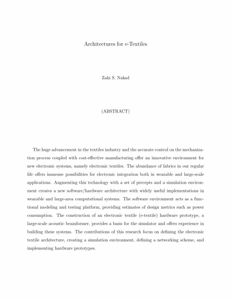
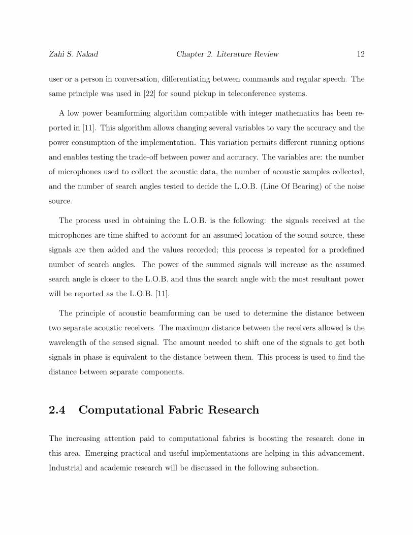
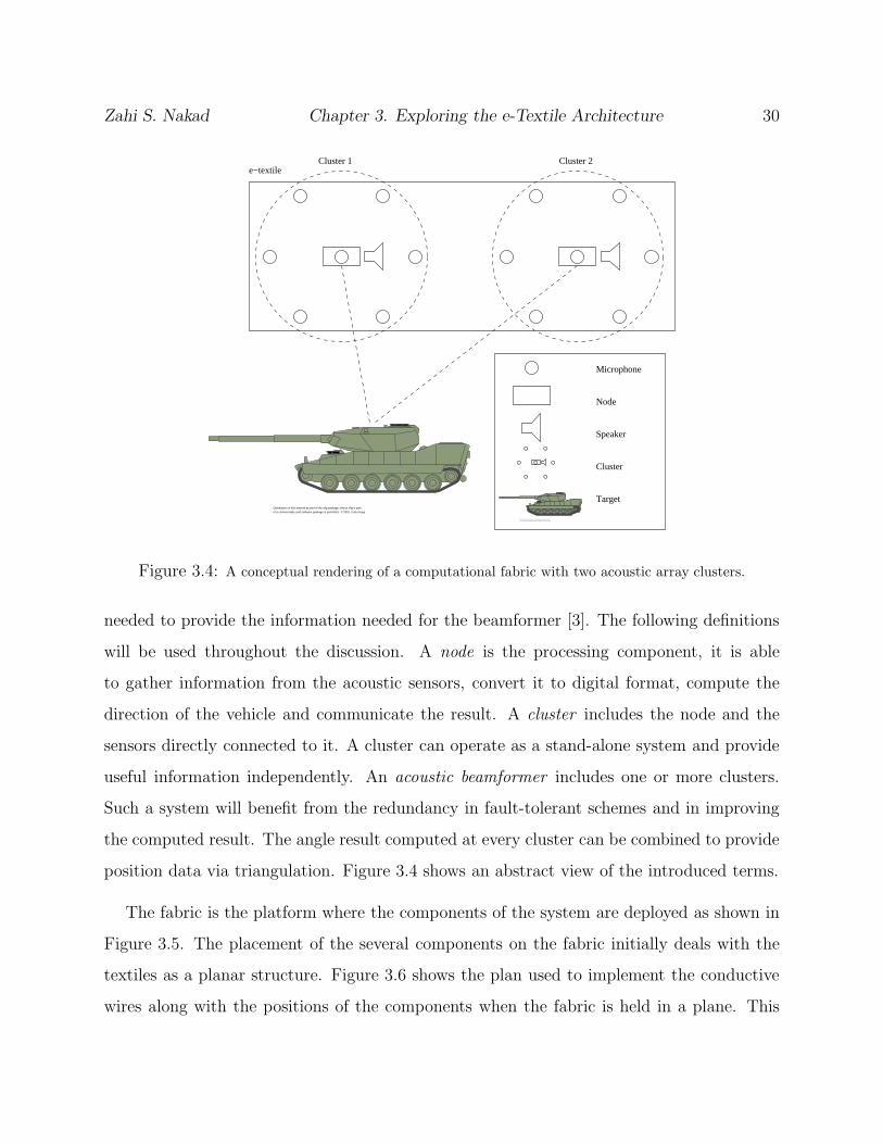
Figure 3.4: A conceptual rendering of a computational fabric with two acoustic array clusters.
needed to provide the information needed for the beamformer [3]. The following definitions
will be used throughout the discussion. A node is the processing component, it is able
to gather information from the acoustic sensors, convert it to digital format, compute the
direction of the vehicle and communicate the result. A cluster includes the node and the
sensors directly connected to it. A cluster can operate as a stand-alone system and provide
useful information independently. An acoustic beamformer includes one or more clusters.
Such a system will benefit from the redundancy in fault-tolerant schemes and in improving
the computed result. The angle result computed at every cluster can be combined to provide
position data via triangulation. Figure 3.4 shows an abstract view of the introduced terms.
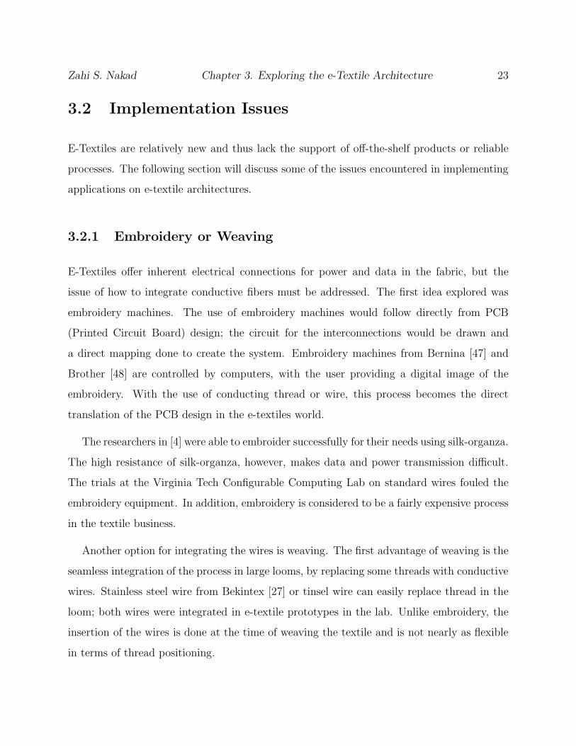
The fabric is the platform where the components of the system are deployed as shown in
Figure 3.5. The placement of the several components on the fabric initially deals with the
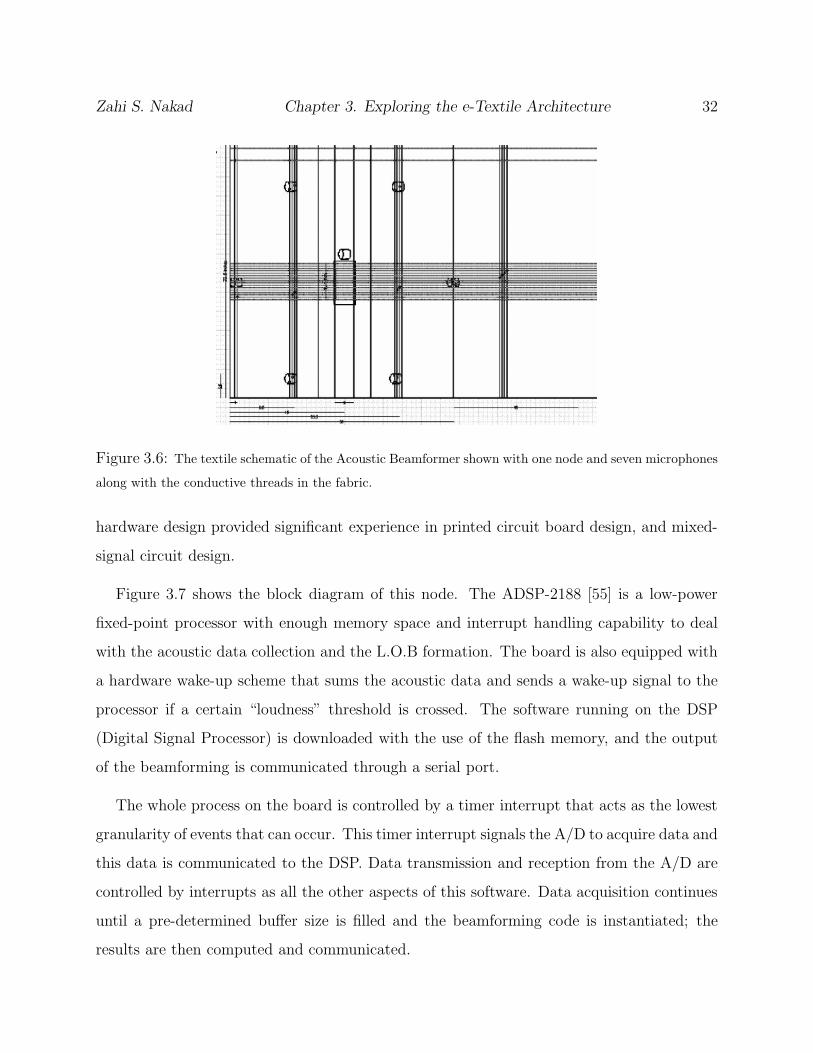
textiles as a planar structure. Figure 3.6 shows the plan used to implement the conductive
wires along with the positions of the components when the fabric is held in a plane. This
Zahi S. Nakad Chapter 3. Exploring the e-Textile Architecture 31
Figure 3.5: The implemented Acoustic Beamforming Array (one cluster) shown on a multi-layer fabric.
diagram was used to help the weaver in creating our fabric prototypes that resulted in the
acoustic beamformer.
In any stand-alone system, power is a major issue. Battery replacement is an impossibility
or a highly improbable luxury; thus, sensing operations on battlefields necessitates power
efficiency. The tasks implemented and the hardware operation should be power-aware; using
approximations and pushing the processors into dormant states. The software running on
the nodes in the implemented 30-foot fabric can force the hardware to a dormant state, the
node will wake up only when there is a significant acoustic signal. A node in this system
can also be awakened by another node in the system by sending a data packet.
3.4.2 Hardware and Software of the Processing Node
The hardware processing node in the acoustic beamformer was designed for this specific
project. The experience gained from its creation had a more general effect. The implemented
interrupt-driven software guided the simulation effort as will be discussed in Chapter 5. The
Zahi S. Nakad Chapter 3. Exploring the e-Textile Architecture 32
Figure 3.6: The textile schematic of the Acoustic Beamformer shown with one node and seven microphones
along with the conductive threads in the fabric.
hardware design provided significant experience in printed circuit board design, and mixed-
signal circuit design.
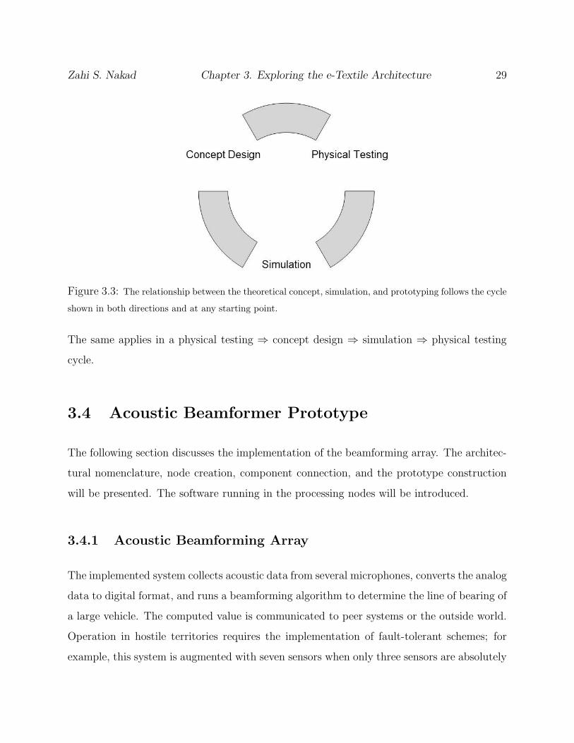
Figure 3.7 shows the block diagram of this node. The ADSP-2188 [55] is a low-power
fixed-point processor with enough memory space and interrupt handling capability to deal
with the acoustic data collection and the L.O.B formation. The board is also equipped with
a hardware wake-up scheme that sums the acoustic data and sends a wake-up signal to the
processor if a certain “loudness” threshold is crossed. The software running on the DSP
(Digital Signal Processor) is downloaded with the use of the flash memory, and the output
of the beamforming is communicated through a serial port.
The whole process on the board is controlled by a timer interrupt that acts as the lowest
granularity of events that can occur. This timer interrupt signals the A/D to acquire data and
this data is communicated to the DSP. Data transmission and reception from the A/D are
controlled by interrupts as all the other aspects of this software. Data acquisition continues
until a pre-determined buffer size is filled and the beamforming code is instantiated; the
results are then computed and communicated.
Zahi S. Nakad Chapter 3. Exploring the e-Textile Architecture 33
Ring 1
Op Amp
Op Amp
A/DDSP
2188M
Flash
Mic 1
Mic 2
Mic 3
Mic 4
Mic 5
Mic 6
Mic 7
2 3 GPS
Figure 3.7: The block diagram of a node shows the interface with the fabric along with the inner connections
Active_Message
SIGTIMER
SIGSPORT0RECV
SIGSPORT0XMIT
SIGSPORT1XMIT
SIGSPORT1RECV
SIGPWRDWN
SIGIRQE
Interrupt
Handler
Timer_Subroutine
Transmission_Subroutine
Serial_Port_Transmission_Subroutine
Serial_Port_Reception_Subroutine
PowerDown
Node_Reception_Subroutine
Timer_Mic_Sampling
Timer_Milli_Second
Timer_Send_To_Node
Timer_Receive_From_Node
Reception_Subroutine
Queue_Get_Message
Transmit
Send_To_Node
Receive_From_Node
Transmit_Result
Queue_Add_Message
Transmit_Request
Transmit_Result_Serial_Only
Data_Manipulation
Figure 3.8: The software block diagram shows the interaction between the interrupts handling routines
and the other functions in the node software.
Zahi S. Nakad Chapter 3. Exploring the e-Textile Architecture 34
The DSP has two generic serial ports, one is used to communicate with the A/D and the
other with a host machine. Sending data between nodes is done with the help of flag pins;
every character to be sent is encoded in a fashion similar to RS-232. The flags send out their
values using the timer interrupt as a synchronization. The reception side is more complex.
Each incoming data line is tied to an interrupt and a data pin (RAM data pin). At the
reception of the first bit (forced to be a 1), the interrupt signals the reception of data and
is disabled until the end of the reception, and the DSP reads the data as if reading from its
memory. The memory reads are also synchronized with the timer interrupt. All nodes have
to run the timer interrupt at the same frequency. A more advanced node would use a DSP
with more communication ports to enable the use of I2C for example. Data packets are
controlled with the use of a general message queue. This queue stores all the packets that
need to be communicated and controls transmission in a FIFO (first-in first-out) fashion.
Figure 3.8 depicts all the interacting parts of the software including the interrupt handlers. A
specific path in this diagram will be scrutinized in detail in Chapter 5 to show the operation
of the simulator alongside the operation of the hardware.
Chapter 4
Electronic Textile Architecture
The work described in Chapter 3 provided the input to create the basis of the Electronic
Textile Architecture. This architecture will derive its precepts from the previous experiences
and show possibilities for future directions. These directions will later be either positively
proved as precepts or negatively dismissed as were previous attempts. This section will
provide an overview of the created precepts and the discarded attempts in relation to tasks
in the creation and implementation of an electronic textile system.
4.1 Embedding of Conductive Channels
An electronic textile is defined as a set of sensors, processors, and actuators embedded in a
fabric backplane interacting to serve a specific goal, with all communication and power lines
integrated in the fabric. The integration of the communication and power lines is integral to
the architecture. This section will discuss the discarded attempts, precepts, and open issues
of the architecture.
35
Zahi S. Nakad Chapter 4. Electronic Textile Architecture 36
4.1.1 Embroidery vs. Weaving
Using weaving as the method for incorporating conductive channels in an electronic textile
was discussed in detail in Section 3.2.1. The conclusions from our experience are:
- Precept: Weaving will be used to incorporate conductive channels. The locations
of these channels will be determined at the outset of the weaving process. Weaving
dictates an X-Y structure in the network.
- Attempt: Embroidery did not prove successful for the type of conductive elements
we are using in this architecture. The embroidery machines were jammed by the used
conductive channels.
4.1.2 Uninsulated vs Insulated Conductors
The choice between insulated and uninsulated wire or conductive channel (will be referred
to as wires until the end of the section) has a great impact on the direction and the design
decisions to be taken. Uninsulated wires provide ease of connection but at a cost. In our
implementation of a beamforming cluster using uninsulated wires we implemented the fabric
in multiple layers; two layers carrying wires either along the length or width of the fabric
and an insulation layer between them. The connection between wires on separate layers goes
through the insulation layer and is fixed mechanically. This type of connection proved to
be unstable. The uninsulated wires provided short circuit risks if the fabric is subjected to
crumpling. Another problem with uninsulated stranded wire is the “fraying” of the strands
as these wires undergo the weaving process in a loom, creating the potential for short circuits.
The use of insulated wires provides the ability to use single layer fabrics, much simpler to
manufacture, but there is the issue of removing the insulation when a connection is needed.
The method of connecting to these wires will be discussed in Section 4.2.1.
- Precept: Use insulated wires to simplify the manufacturing of the fabric while devising
Zahi S. Nakad Chapter 4. Electronic Textile Architecture 37
better wire connection techniques.
- Attempt: Use of uninsulated wires was not successful for the above mentioned reasons.
4.1.3 Conductive Material
The different types of wires in an electronic textile has been discussed in detail in Sec-
tion 3.2.1. The conclusions are as follows:
- Precept: The properties of the tinsel wire combines flexibility, conductivity, and sol-
derability. The insulation on these wires is detergent resistant and thus can withstand
cleaning the fabric.
- Attempt: Single strand wire did not provide the needed flexibility and at high gauges
it was susceptible to breakages. The Bekintex wire has a tendency to “fray” which can
introduce short circuits.
- Open Issues: More research and experimentation is required on the use of conductive
polymers to determine their utility in carrying power, analog data, and digital data.
4.1.4 Analog vs Digital Signals
The question of sending analog or digital signals on the wires is application dependent, but
there are aspects that can be generalized. Analog transmission is more prone to noise and
interference, but we were successful with the acoustic beamformer due to the low sampling
rates and the low communication speeds on other lines in the fabric. Interference will have
a higher impact in a motion sensing vest, for example, that incorporates cameras and/or
antennas.
Using digital communication for all the signals on an electronic textile will provide a more
stable system, along with pushing analog processing of the data closer to the sensors. The
Zahi S. Nakad Chapter 4. Electronic Textile Architecture 38
processing nodes will only receive digital signals in this setup. Using I2C, for example, for
all signal communications eases the general design of the system. When a specific standard
is tested and then used for all consequent applications, the number of variables in a system
is reduced. For example I2C forces the use of four wires for any communication channel,
thus any channel in the fabric should consist of four wires throughout. Digital transmission,
on the other hand, adds the cost of analog/digital conversion and communication hardware
to each sensor.
- Precept: Digital transmission should be used for all of the signals on such a system.
- Attempt: Analog transmission can also be used, but is not recommended.
4.1.5 Communication Busses
Following the previous discussion, digital signals will be used throughout an electronic textile
system. The use of I2C busses throughout helps in standardizing the layout of the fabric as
can be seen in Figure 4.1 which represents a unit of the fabric used in creating the textile
component of the Shape Sensing project [50]. The wires are implemented in sets of four
to carry all the signals of the busses, and these busses are repeated to generalize the fabric
created and to provide support for future endevours using the same fabric. The fabric used in
the Acoustic Beamformer was specifically designed for that project and cannot be configured
for other implementations.
- Precept: Use a standard bus communication method for all signals in the fabric to
help in generalizing the fabric design.
- Attempt: Design the fabric for the specific application results in a loss of re-usability.
Zahi S. Nakad Chapter 4. Electronic Textile Architecture 39
Figure 4.1: Schematic of a unit of fabric of the textile used in creating the shape sensing pants [56].
Zahi S. Nakad Chapter 4. Electronic Textile Architecture 40
4.2 Manufacturability
The following section will discuss parts of the architecture that will help in creating a manu-
facturable electronic textile. The issues discussed address component/fabric connectors and
a more general node design.
4.2.1 Fabric/Component Connectors
The connection between the components of the electronic textile and the fabric is harder
than the straight-forward problem it seems to be. The following subsections will discuss
the approaches used in the Acoustic Beamformer and the Shape Sensing projects and will
provide insight into the creation of the needed connectors.
Soldering vs. Mechanical Connection
The first approach used with insulated wire was the use of standard 2mm header pins,
stripping the insulation off regular wires and soldering. The solder is not flexible and when
used on the fabric it was prone to breaking and open circuits. Solder also cannot be used with
the stainless steel wire. Another approach was the use of conductive epoxy which provided
the needed flexibility but it proved cumbersome and did not provide the needed strength for
the physical connection. Mechanical means of connections with the use of knives to remove
the insulation seem to be the best solution. These connectors can work with many types of
wires, provide the needed physical support, and are easily mechanized.
- Precept: Use mechanical means for connections similar to insulation displacement
connectors (mechanized connectors still need to be designed).
- Attempt: The use of solder or conductive epoxy was not totally successful nor totally
merchandisable.
Zahi S. Nakad Chapter 4. Electronic Textile Architecture 41
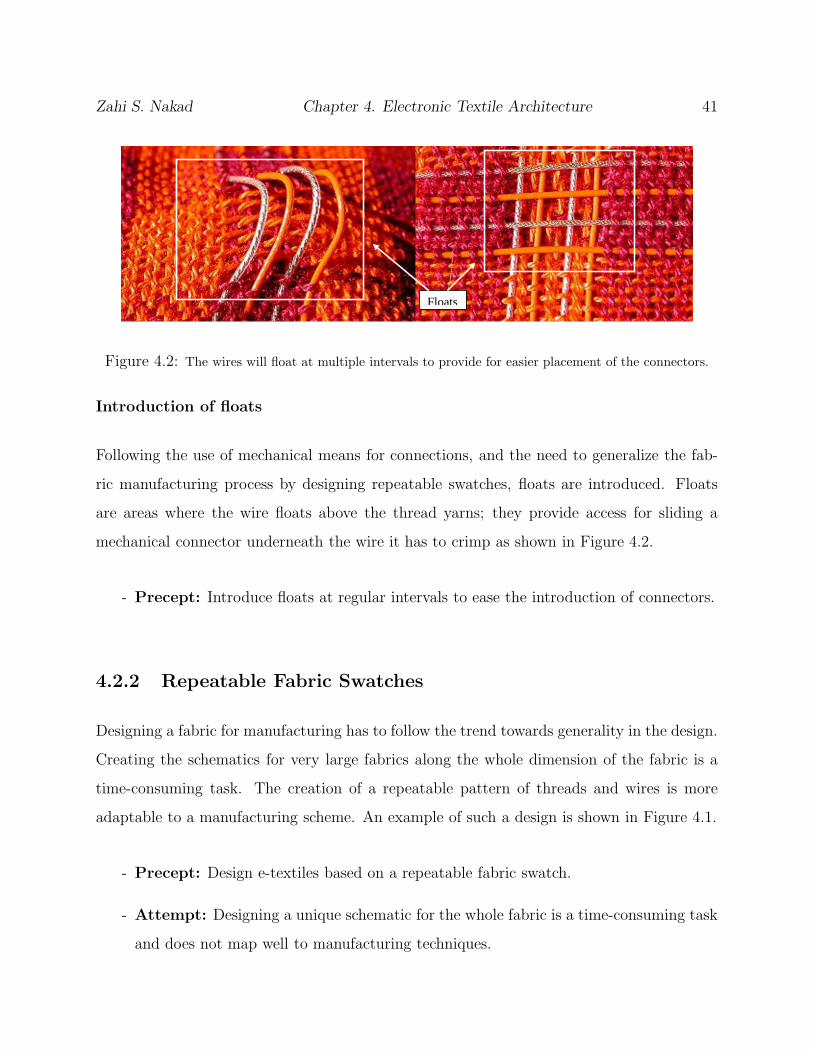
Floats
Figure 4.2: The wires will float at multiple intervals to provide for easier placement of the connectors.
Introduction of floats
Following the use of mechanical means for connections, and the need to generalize the fab-
ric manufacturing process by designing repeatable swatches, floats are introduced. Floats
are areas where the wire floats above the thread yarns; they provide access for sliding a
mechanical connector underneath the wire it has to crimp as shown in Figure 4.2.
- Precept: Introduce floats at regular intervals to ease the introduction of connectors.
4.2.2 Repeatable Fabric Swatches
Designing a fabric for manufacturing has to follow the trend towards generality in the design.
Creating the schematics for very large fabrics along the whole dimension of the fabric is a
time-consuming task. The creation of a repeatable pattern of threads and wires is more
adaptable to a manufacturing scheme. An example of such a design is shown in Figure 4.1.
- Precept: Design e-textiles based on a repeatable fabric swatch.
- Attempt: Designing a unique schematic for the whole fabric is a time-consuming task
and does not map well to manufacturing techniques.
Zahi S. Nakad Chapter 4. Electronic Textile Architecture 42
4.2.3 Smaller More General Nodes (Beamformer vs e-TAGS)
The design direction of sending all signals on digital busses spread in a regular pattern over
the textile pushes the design space into the creation of more general processing nodes. There
will be a need for sensor data processors that will convert the analog data and provide the
communication interface. The generalization of these nodes will lead to the manufacturing
of “sensor nodes” that can be tuned to the specific sensor. This path diverts from the
first approach of designing a specific node for a specific job as was done with the Acoustic
Beamformer. The same concept can be applied to the processing nodes. The creation of
the more general nodes will decrease the price of manufacturing and designing by using a
mass production approach, and will map better to the approach of standardizing all signal
transmissions on these systems. This approach is under research in the e-TAGS project [51].
- Precept: Move to generalizing the nodes in the electronic textile.
- Attempt: The creation of specific nodes for specific jobs is too expensive.
4.2.4 Classes of Nodes
With the development of the electronic textile architecture and technology, two classes of
nodes will arise. Sensor nodes that use simple microcontrollers will become smaller and will
ultimately be integrated in the fabric. Communication hubs and processing nodes will get
more powerful with technology advances.
- Precept: The architecture can be used to develop applications that will map to pre-
dicted technology advances and to the different classes of nodes.
Zahi S. Nakad Chapter 4. Electronic Textile Architecture 43
4.3 Software
This section will provide the aspects of the software part of the the architecture. These
aspects are provided in the simulation environment. The implementation in the software
environment forces the simulated processes to follow these precepts by using the provided
services.
4.3.1 Interrupt Driven Processing
An electronic textile system will most probably deal with sensing certain physical phenomena
and react according to pre-determined procedures. Interrupt driven processing maps directly
to such a situation; a processor will not process unless it receives data (interrupt event),
sensor nodes will not report unless there is a significant action (interrupt event) and so
forth. The simulator provides a core simulator of a processor that is able to process interrupts
and respond accordingly. The simulated operation of the system can easily be moved to a
hardware installation with an interrupt driven processor. This applies to the ADSP-2188
used in the Acoustic Beamformer and the microcontrollers used in the e-TAGS.
- Precept: Interrupt driven processing maps to the hardware process and the sensed
phenomena and thus will be the processing model used in the architecture.
4.3.2 Fault-Tolerant Communication Scheme
The use of electronic textile systems in harsh environments will introduce faults in the system.
Such a stand-alone system should be able to withstand such faults and continue operation
perhaps with decreased functionality. The electronic textile architecture will provide a fault-
tolerant communication scheme that will route around faults. The network will be discussed
in great detail in Chapter 6. The provided network will also map to the X-Y topology of a
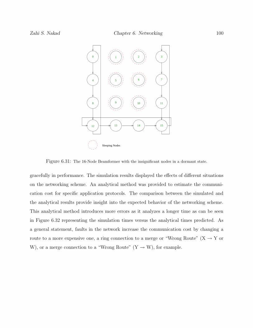
weave and provide the support for “sleeping” nodes.
Zahi S. Nakad Chapter 4. Electronic Textile Architecture 44
- Precept: Provide a communication scheme that maps to the geometry of the weave
and provides a fault-tolerant scheme.
4.3.3 Human Motion Databases for Prototyping
The electronic textile architecture provides the ability to simulate a textile. For wearable
systems, this architecture will provide the ability to test the design on a large number of
people through the use of human motion databases available from [57], for example. An
operational testing phase follows the creation of a prototype. The results of these tests
are more credible because of the large number of test subjects. This architecture provides
means for testing an e-textile prototype by using these human motion databases and thus
providing access to a large number of test subjects to verify the operation of the prototype
or its concept.
- Precept: Use a larger number of subjects to better test the prototype during both
the conception and development stages.
- Attempt: The lack of ability to test a system before it is created in hardware can
prove to be expensive, and testing on a small population can present misleading or
biased results.
4.3.4 Component Distance Finding
The shape of an electronic textile system can change during its operation, thus causing the
distances between the components in the system to vary. The importance of this variation
is application dependent. The hardware implementation of the distance finding process was
achieved. The full integration into the architecture will be accomplished at a later stage for
the specific applications.
Zahi S. Nakad Chapter 4. Electronic Textile Architecture 45
- Precept: Integration of distance finding capabilities into the electronic textile ar-
chitecture will be done for applications where it is crucially required. The current
prototypes have not required these capabilities.
The electronic textile architecture provides a structure and a path to be followed by
new prototype endeavors. This architecture also provides a simulation environment to test
concepts and improve extant hardware applications. A direction towards generality in the
design to reach a more manufacturable technology is also conveyed; the weave design should
allow for the creation of multiple sizes and types for different applications. Using a standard
communication scheme, for example, will help in simplifying the hardware nodes and the
communication portion of the design.
Chapter 5
Simulation
Our goal is to create an e-textile architecture that is accessible to future researchers. At
the outset of a project, implementing every aspect of an e-textile system in hardware can
be expensive and time consuming. Creating a software environment that simulates the
operation of e-textile systems can be extremely beneficial by allowing the design space to be
explored without having to build a prototype. Such a simulation environment can be used
to enhance the performance of extant systems as well.
Writing a simulation package from scratch is a major task and thus we decided to use
an available one. Ptolemy [19] was chosen because it is designed to simulate heterogeneous
and embedded systems. The created environment will be discussed by showing its operation
in regards to the system described in Section 3.4. This chapter will describe the different
aspects of the simulator and will demonstrate its general usability, Section 5.1. With Ptolemy
we are able to simulate the interaction with the outside world and the response created
from the e-textile system. This chapter will discuss the simulation of the acoustic signals
created by a large vehicle at a specific location with respect to each microphone, Section 5.2.
The discussion will also cover the simulation of computing the result of the beamformer
code, Section 5.3 along with the operation of this code while communicating with other
nodes in the system Section 5.5. Power consumption is another aspect that the environment
46
Zahi S. Nakad Chapter 5. Simulation 47
reports to help in evaluating e-textile stand-alone systems, Section 5.4. The disucssion of the
communicatgion simulation is provided in Section 5.5. The integration of the fault simulation
and the communication scheme is discussed in Section 5.6 The creation of a hybrid mode of
simulation will also be discussed, Section 5.7; this mode allows the simulation environment
to interact with the actual hardware of the simulated system in a full or partial manner.
This mode helps in grounding the results obtained. Finally, Section 5.8 discusses fine-tuning
the Acoustic Beamformer using the simulator.
5.1 Simulator Architecture
The simulation environment simulates different aspects of an e-textile system and the phys-
ical world it interacts with. The following is a listing of the simulator parts that deal with
these aspects:
- Physical World: This represents the simulation of the physical world that is sensed or
interacted with by the simulated e-textile prototype. Simulations of the physical world
are usually done in the CT domain (Continuous Time). This simulator interacts with
the interrupt handling core to mimic the operation of a hardware system. Simulation
of the physical world also includes simulating the faults that occur on the fabric and
provide the disruptions in power or communication caused by these faults. The faults
simulation is controlled by the DE domain (Discrete Event).
- Interrupt Handling Core: According to the developed precepts on software, the
core of an e-textile prototype operates using interrupt driven processing. This model
of operation is provided in the simulator along with interacting with the physical world
simulator. This simulator is managed by the DE domain (Discrete Event) and provides
its operational states to the power simulator to create power consumption values.
Zahi S. Nakad Chapter 5. Simulation 48
- Power Simulation: The power simulator collects the power state information from
the core simulator. By tracking the states of operation the power simulator provides
power consumption values in the whole system. This simulator is controlled by the DE
domain (Discrete Event).
5.2 Physical World
The discussion of the physical world simulator will follow the simulation process of the
Acoustic Beamforming Array. Every node on the array processes acoustic data received by
its microphones. The first step in the simulation is creating these acoustic signals according
to the simulated position of the vehicle. The acoustic signals are attenuated and phase
shifted according to the location of the microphones on the fabric. The details of creating
these simulated signals are provided in [53]. The Continuous Time (CT) domain was used
to simulate the position of the vehicle and the created acoustic response at each microphone.
This data is passed to the interrupt handling core at the request of the simulated node.
The operation of the node is controlled by the Discrete Event (DE) domain as discussed in
Section 5.3. Ptolemy provides the ability to combine simulators running in different domains;
a list of these domains was provided in Section 2.2.1. The simulation of the physical world
includes information about faults (fabric tears) that can be induced in the fabric; that aspect
of the simulation will be discussed in Section 5.6.
5.3 Interrupt Handling Core
The interrupt handling core was used to simulate the operation of the DSP part of the
Acoustic Beamforming Array. The current hardware acoustic beamformer includes four
independent clusters that can provide a line of bearing for a moving vehicle. Each cluster
depends on the processing node for the computation of the line of sight. The implementation
Zahi S. Nakad Chapter 5. Simulation 49
of this prototype was discussed in detail in Section 3.4.
The simulator for this beamformer duplicates the operation of the node, which include:
acoustic data collection, computation of the line of bearing, communication with the other
nodes in the system, and triangulation of the obtained lines of bearing (from separate nodes)
to determine position data. The simulator for the node reports a power state so that the
power simulator can calculate the power consumed; the implementation of the power simu-
lator will be discussed in more detail in Section 5.4.
SIGTIMER
SIGSPORT0RECV
SIGSPORT0XMIT
SIGSPORT1XMIT
SIGSPORT1RECV
SIGPWRDWN
SIGIRQE
Interrupt
Handler
Timer_Subroutine
Transmission_Subroutine
Serial_Port_Transmission_Subroutine
Serial_Port_Reception_Subroutine
PowerDown
Node_Reception_Subroutine
Timer_Mic_Sampling
Timer_Milli_Second
Timer_Send_To_Node
Timer_Receive_From_Node
Reception_Subroutine
Queue_Get_Message
Transmit
Send_To_Node
Receive_From_Node
Transmit_Result
Queue_Add_Message
Transmit_Request
Transmit_Result_Serial_Only
Data_Manipulation
Active_Message
Figure 5.1: The abstract implementation of the simulator includes C code from the hardware implemen-
tation, JAVA code from the Ptolemy environment, and the JNI (Java Native Interface) [58] in between
(Interrupt Handler). The thick lines highlight the advancement through the code following the description
in Table 5.1
Ptolemy provides a heterogeneous simulation environment targeted at the simulation
of embedded systems. Ptolemy can represent systems that mix different technologies and
devices [19]. This environment imposes some structure on the simulated systems; the com-
ponents have to be encapsulated in Ptolemy actors and the interactions of these components
are controlled by a “model of computation,” with several models provided. The acoustic
beamformer simulator (interrupt handling core) utilizes the DE (Discrete Events) model.
Zahi S. Nakad Chapter 5. Simulation 50
Figure 5.2: The node simulator in Ptolemy, this node connects using ports to other nodes in the network
and interacts with the acoustic data simulator (truck).
The DE domain matches the interrupt-driven operation of the DSP in the node. This model
governs the timing of events occurring in the simulation environment. These events include:
timer interrupts, acoustic data collection, and line of bearing communication.
The Ptolemy environment is written in JAVA and so are the actors to be created by the
users. The generation of the line of sight and interrupt handling at the DSP are implemented
in C; the JNI is used as a link between them and the actor simulating the DSP operation
in Ptolemy. Figure 5.1 (repetition of Figure 3.8) is a block diagram depicting the code
implemented on the node. Each block is either implemented in C (native code from the DSP
implementation) or Java (code simulating the operation of the DSP code in the hardware
implementation and the interface between the Ptolemy environment and the other simulation
elements). The number of interrupts implemented and their names are specific to the DSP
used, the Analog Devices ADSP-2188, but this environment, the interrupt handling core, can
be used as a general interrupt-driven processing element simulation. The whole simulation
is driven by a periodic signal (Timer interrupt in this case); it checks for interrupts received
and services these interrupts according to a pre-specified priority scheme. This simulation
Zahi S. Nakad Chapter 5. Simulation 51
aims at proving functionality and providing a power consumption estimate for the prototype.
The node simultor in Ptolemy is shown in Figure 5.2.
The operation of the simulation will be explained by focusing on a small but representative
part of the code and discussing it in detail. The acoustic data collection shown in Table 5.1
will be used as this representative part because it uses most of the aspects of the simulator
implementation.
5.4 Power Simulation
Rate of power consumption is a crucial measure in stand-alone applications. Simulating
power consumption provides a useful means of varying the operation of an application to
reach a more efficient performance in terms of consumed power. Each processing node can
be operating in one of a set of operation phases. The interrupt handling core reports these
states to the power simulator.
In the Acoustic Beamforming Array, the processing node can be collecting data from the
microphones, performing the beamforming operation, communicating with other nodes in
the fabric, or waiting in the idle state. Physical measurements were performed to collect the
power consumed in these phases. Using these basic values, the parameters of the system can
be changed such as number of microphones and the power consumption values simulated.
Each node in the simulation provides information about its processing states, a power tracker
tracks these changes and based on the measured values computes the power consumption of
the system. Multiple tables in [54] document this simulated data. These tables provide in-
formation about the operation of the prototypes under varying circumstances. The Acoustic
Beamforming Array was the prototype in [54].
This simulation environment was used in [46] to provide energy consumption values while
varying system parameters.The large increase in power consumption values when using wire-
less communication, reported in [46], shows the advantage of using e-textiles in large-area
Zahi S. Nakad Chapter 5. Simulation 52
Table 5.1: Acoustic Data Collection
Block Implementation Function
SIGTIMER Ptolemy The timer interrupt is created in the DSP bya dedicated counter. A clock is used in thesimulation environment. This timer controls allthe processes in the simulation (and hardware);specifically triggering the request for acousticdata.
Interrupt Handler JAVA This block simulates the interrupt handling inthe DSP, it keeps a record of the received inter-rupts until served and branches to the requiredsubroutine. The acoustic data request (trans-mit and receive) interrupts are handled here.
Timer Subroutine C The Interrupt Handler branches the operationto Timer Subroutine when the SIGTIMER in-terrupt is to be handled. This subroutine trig-gers all scheduled events including the requestfor the acoustic data.
Timer MicSampling
C The branch inside the Timer Subroutine thatdeals with sampling the acoustic data.
SIGSPORT0XMIT Ptolemy The interrupt received at the transmission ofthe acoustic data request.
TransmissionSubroutine
C Sends the request for data from the mic thatwill be sampled next.
SIGSPORT0RECV Ptolemy The interrupt received at the reception of anacoustic data word.
ReceptionSubroutine
C-JAVA Receive the data from the queried mics andkeep track of filling the buffers of the acousticdata
Zahi S. Nakad Chapter 5. Simulation 53
sensing applications. A study of prolonging the operation of the Acoustic Beamforming
Array by changing the number of power sources and dealing with faults in the power lines
and the processing nodes was presented in [54] using this power simulator. The simula-
tor descibed in Section 5.3 was used in conjuction an actor providing the fault information
(Physical Model) and another actor tracking the power consumption (Power Tracker) to
provide needed simulation [54].
5.5 Communication Simulation
Testing the implemented communication scheme through prototyping will require building
enough hardware prototypes to significantly explore its operation. Simulation of multiple
communicating nodes is more feasible and is viable with the use of the developed simulator.
Figure 5.3 depicts a basic setup of two grids of 16 nodes each connected with a set of trans-
verse links (these links are discussed in detail in Chapter 6). Creating all the connections
by hand for each of the present ports is labor intensive. The representation of the connec-
tions in Ptolemy is done with XML (Extensible Markup Language) [60]. With the use of
XML, large networks and the links between them can be created automatically. Automatic
code generation provides a useful medium for testing different applications and computing
performance metrics, as will be done in Section 6.5.
5.6 Integrating the Fault Simulation and the Commu-
nication Scheme
The communication scheme used in the system will be described in Chapter 6. This scheme
can route around faults and sleeping nodes. The physical world simulator provides support
to test this implementation by attaching a Fabric actor to the actor simulating a node in
the Acoustic Beamforming Array. The Fabric actor shown in Figure 5.4 creates the error
Zahi S. Nakad Chapter 5. Simulation 54
Figure 5.3: Simulation of 32 nodes on two separate grids joined with transverse links.
information that blocks data from crossing the communication channels that exist on the
fabric. This is done by controlling multiplexors through the control signal provided. The
Fabric actor also recognizes that an error in the communication channel can be to the “left”
or the “right” of a node, or on the channel providing the link between the nodes at the ends
of the ring. These channels are depicted in a block diagram in Figure 5.5. When a channel
is disconnected a node detects this error and the fault tolerant process in the networking
scheme deals with the error as discussed in Chapter 6. Figure 5.6 presents the simulator
for the Acoustic Beamforming Array while using these nodes. More communication links
are used in this case to account for the links traversing the ring between the edges. The
physical world simulator was also used in [54] to test for power line disruptions caused by
the introduced faults.
Zahi S. Nakad Chapter 5. Simulation 55
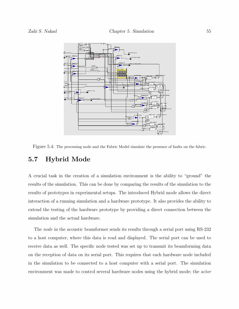
Figure 5.4: The processing node and the Fabric Model simulate the presence of faults on the fabric.
5.7 Hybrid Mode
A crucial task in the creation of a simulation environment is the ability to “ground” the
results of the simulation. This can be done by comparing the results of the simulation to the
results of prototypes in experimental setups. The introduced Hybrid mode allows the direct
interaction of a running simulation and a hardware prototype. It also provides the ability to
extend the testing of the hardware prototype by providing a direct connection between the
simulation and the actual hardware.
The node in the acoustic beamformer sends its results through a serial port using RS-232
to a host computer, where this data is read and displayed. The serial port can be used to
receive data as well. The specific node tested was set up to transmit its beamforming data
on the reception of data on its serial port. This requires that each hardware node included
in the simulation to be connected to a host computer with a serial port. The simulation
environment was made to control several hardware nodes using the hybrid mode; the actor
Zahi S. Nakad Chapter 5. Simulation 56
0
0
0
0
0
0
0
0
0
Processing
Node
Fabric
Model
ROW
ROW
ROW
COLUMN
COLUMN
COLUMN
TRANSVERSETRANSVERSE
TRANSVERSE
Figure 5.5: Multiplexors controlled by signals from the Fabric Model create the errors in the communication
links.
Figure 5.6: Extra connections to the new node, Figure 5.4, are required to represent the connections.
Zahi S. Nakad Chapter 5. Simulation 57
RS−232
TCP
Figure 5.7: Using an X terminal, the simulation can be run on a server that connects through TCP to
host computers controlling hardware nodes to be used in a “Hybrid Mode” simulation.
representing the hardware node creates a TCP connection to the host computer controlling
the hardware node; the set up is shown in Figure 5.7, allowing the connection of several
hardware nodes, limited by the number of host machines and nodes.
The hardware testing of a communication protocol on a large network is more feasible
using this mode than using a large network of hardware nodes, thus compensating for a low
number of hardware prototypes.
5.8 Fine-Tuning the Beamformer
The simulation environment provides a virtual space for designing and testing e-textile pro-
totypes. This simulation environment was used extensively to test the results of the Acoustic
Beamformer in [53]. The results of each node were tested with varying specific parameters;
an example result shows the maximum error in the angle estimation with varying the number
Zahi S. Nakad Chapter 5. Simulation 58
Processing Node
Sensing Element
Node to Node Link
Sensor to Node Link
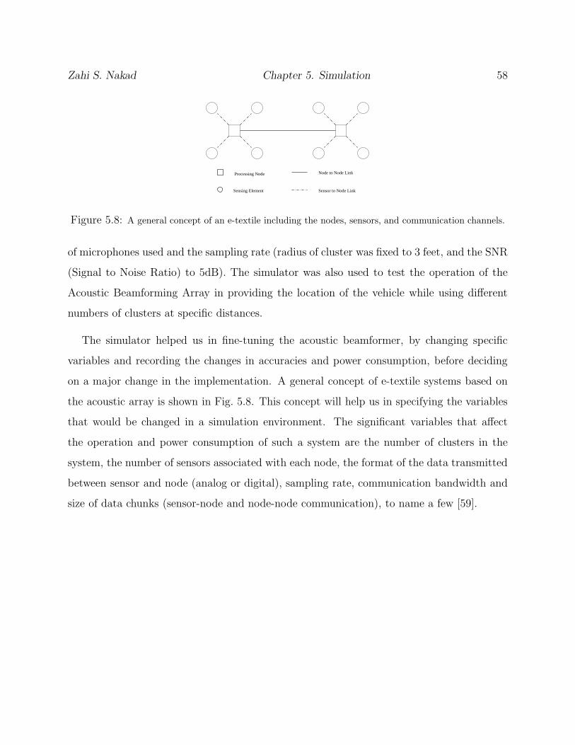
Figure 5.8: A general concept of an e-textile including the nodes, sensors, and communication channels.
of microphones used and the sampling rate (radius of cluster was fixed to 3 feet, and the SNR
(Signal to Noise Ratio) to 5dB). The simulator was also used to test the operation of the
Acoustic Beamforming Array in providing the location of the vehicle while using different
numbers of clusters at specific distances.
The simulator helped us in fine-tuning the acoustic beamformer, by changing specific
variables and recording the changes in accuracies and power consumption, before deciding
on a major change in the implementation. A general concept of e-textile systems based on
the acoustic array is shown in Fig. 5.8. This concept will help us in specifying the variables
that would be changed in a simulation environment. The significant variables that affect
the operation and power consumption of such a system are the number of clusters in the
system, the number of sensors associated with each node, the format of the data transmitted
between sensor and node (analog or digital), sampling rate, communication bandwidth and
size of data chunks (sensor-node and node-node communication), to name a few [59].
Chapter 6
Networking
A networking scheme designed for e-textile applications will be discussed in this chapter.
The scheme is based on the Token Grid described in Section 2.1.2. The modifications to this
network are based upon the precepts stated in the electronic textile architecture detailed in
Chapter 4.
The number of hops a token has to traverse is directly related to the number of nodes
on the ring. In the case of large area e-textiles, a large number of nodes in a ring can slow
the communication on the ring. Fabric swatches will be connected to form large or wearable
fabrics (precept of the electronic textile architecture); the networks on these different fabrics
must be connected. The addition of a third dimension to the networking scheme to address
both of these issues will be discussed in Section 6.1.
Fault tolerance was integrated in the design of the networking scheme in accordance with
the fault-tolerant communication scheme precept. The new fault-tolerance scheme differs
from the Token Grid scheme for two main reasons. First, the Token Grid scheme assumes
no faults on the communication links. Second, the Token Grid scheme assumes that the
processing nodes will have the ability to forward data in the case of a failure. Both of these
assumptions do not apply to e-textiles and thus a new scheme, presented in Section 6.2,
59
Zahi S. Nakad Chapter 6. Networking 60
0 1 2 3
5 6 7
10 11
13 14 15
8
4
9
12
0 1 2 3
5 6 7
10 11
13 14 15
8
4
9
12
GRID 0 GRID 1
Figure 6.1: The new grid architecture has an added “transverse” ring.
was designed. Low-power operation of electronic textile systems dictates the support for
“sleeping” nodes; the networking scheme avoids waking these nodes up unless necessary,
this support is discussed in Section 6.3. Section 6.4 will provide a framework to be used in
reporting the performance of the networking scheme under different conditions in Section 6.5.
6.1 Transverse Dimension
The use of weaving (precept of the electronic textile architecture) inherently forces an X-Y
formation on the fabric; this formation fits the Token Grid network. A new dimension was
added to the grid because the number of nodes in one ring cannot be increased indefinitely.
Figure 6.1 shows the new grid architecture, where each grid of nodes will be connected to
a similar grid. This increase adds to the ability of the system to support large numbers of
nodes. Some nodes get duplicated direct connections and more indirect routes are available
to increase fault tolerance. The potential number of network interfaces of each node in the
new grid, the Textile Token Grid, must be increased. In the original token grid each node
required two outputs and two inputs; this new system requires up to three outputs and three
inputs.
In applying the new grid architecture to physical fabrics, the transverse dimension can
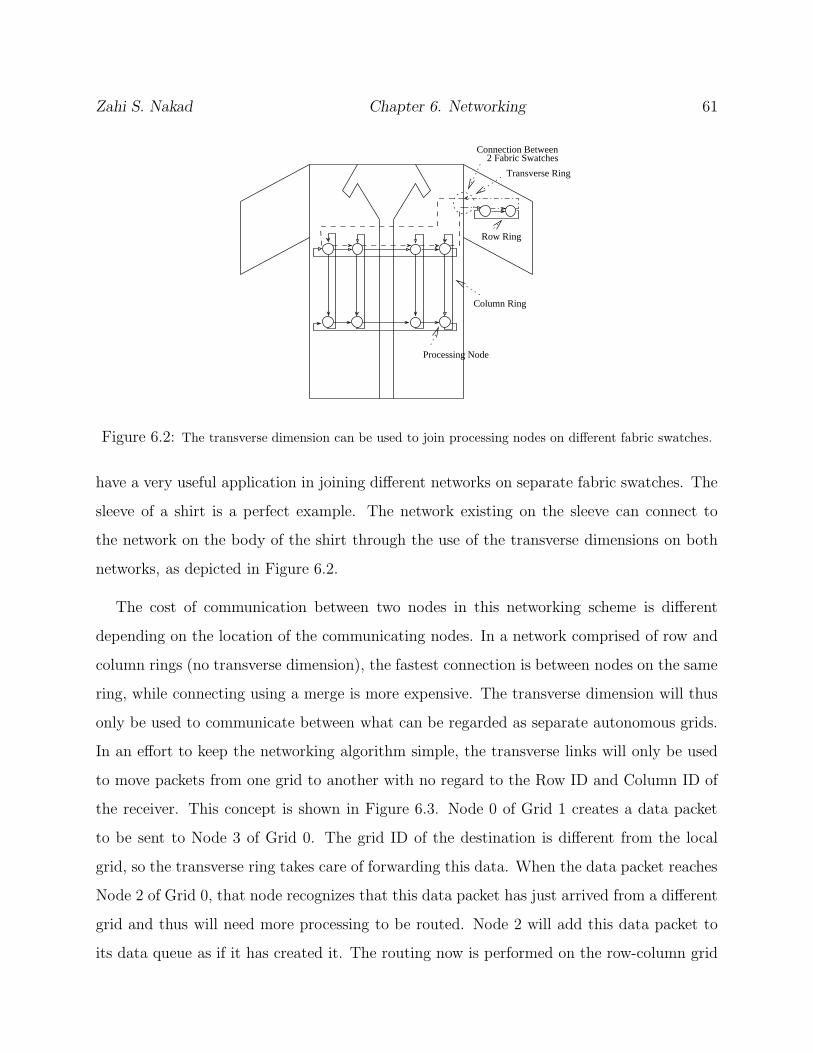
Zahi S. Nakad Chapter 6. Networking 61
Transverse Ring
Processing Node
Row Ring
Column Ring
Connection Between2 Fabric Swatches
Figure 6.2: The transverse dimension can be used to join processing nodes on different fabric swatches.
have a very useful application in joining different networks on separate fabric swatches. The
sleeve of a shirt is a perfect example. The network existing on the sleeve can connect to
the network on the body of the shirt through the use of the transverse dimensions on both
networks, as depicted in Figure 6.2.
The cost of communication between two nodes in this networking scheme is different
depending on the location of the communicating nodes. In a network comprised of row and
column rings (no transverse dimension), the fastest connection is between nodes on the same
ring, while connecting using a merge is more expensive. The transverse dimension will thus
only be used to communicate between what can be regarded as separate autonomous grids.
In an effort to keep the networking algorithm simple, the transverse links will only be used
to move packets from one grid to another with no regard to the Row ID and Column ID of
the receiver. This concept is shown in Figure 6.3. Node 0 of Grid 1 creates a data packet
to be sent to Node 3 of Grid 0. The grid ID of the destination is different from the local
grid, so the transverse ring takes care of forwarding this data. When the data packet reaches
Node 2 of Grid 0, that node recognizes that this data packet has just arrived from a different
grid and thus will need more processing to be routed. Node 2 will add this data packet to
its data queue as if it has created it. The routing now is performed on the row-column grid
Zahi S. Nakad Chapter 6. Networking 62
0 1 2 3
5 6 7
10 11
13 14 15
8
4
9
12
RegularNode
Merged Node Route
Wrong
0 1 2 3
5 6 7
10 11
13 14 15
8
4
9
12
GRID 0 GRID 1
Figure 6.3: The transverse and the row links are used to send packets between Node 0 (Grid 1) and Node
3 (Grid 0).
with no reference to the transverse dimension. This data is then routed to Node 3 of Grid
0 on the row ring. Figure 6.4 displays another case where the data packet is destined for
another grid. Node 2 of Grid 0 had to request a merge from Node 6, and the data was routed
through that merge to Node 7 of Grid 0.
In both cases, Node 2 of Grid 0 added the data packet to its data queue when it did not
have enough information or capability to route that packet without grabbing a token. This
technique, of adding to the data queue, will be used in the fault tolerant scheme described
in Section 6.2.
Each transverse ring traverses two different grids, the transverse token will keep a record
of these grid IDs. In the case that the destination is on a grid other than the source, there
exist two options. The first is to send the data packet on the transverse ring if it can reach
the needed grid. The second is to use the row ring to reach a node connected to the other
transverse ring. This decision will be taken with the help of a routing table. The construction
of this routing table will be dependent on the application and will not be discussed in this
Zahi S. Nakad Chapter 6. Networking 63
0 1 2 3
5 6 7
10 11
13 14 15
8
4
9
12
RegularNode
Merged Node Route
Wrong
0 1 2 3
5 6 7
10 11
13 14 15
8
4
9
12
GRID 0 GRID 1
Figure 6.4: The data packet is treated as a new packet inside the receiving grid. Node 0 Grid 1 uses the
transverse ring to reach Node 2 Grid 0, at Node 2 the packet is re-processed for routing and it is sent through
a merge to Node 7 Grid 0.
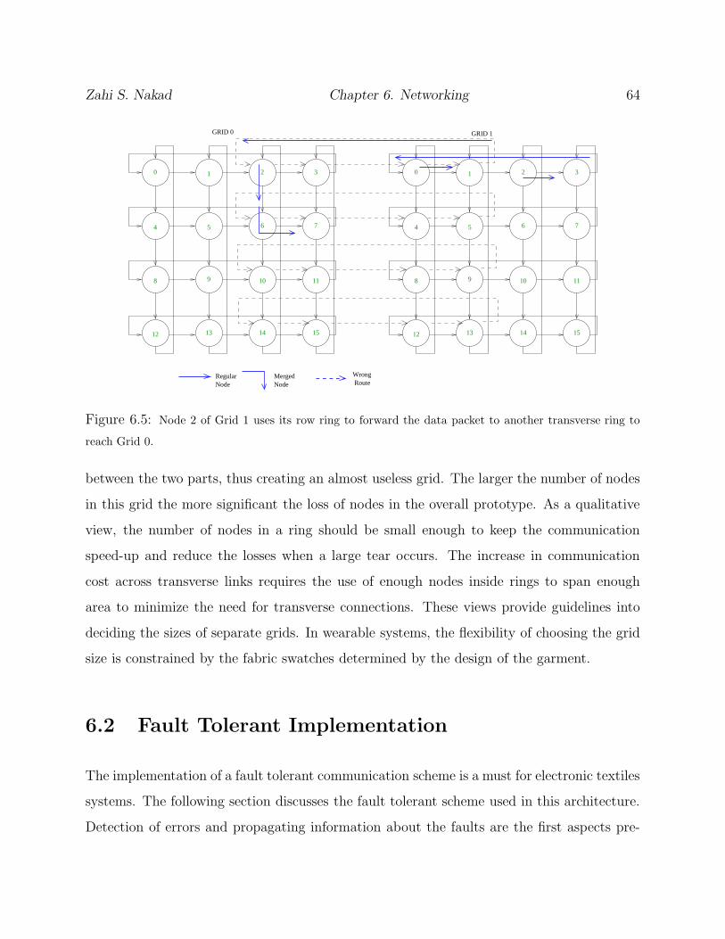
dissertation. Figure 6.5 depicts a case where the row ring is needed before the data packet
can reach the destination grid.
6.1.1 Size of the Grid
The size of the grid dictates the number of nodes in the rings. This is a decision metric that
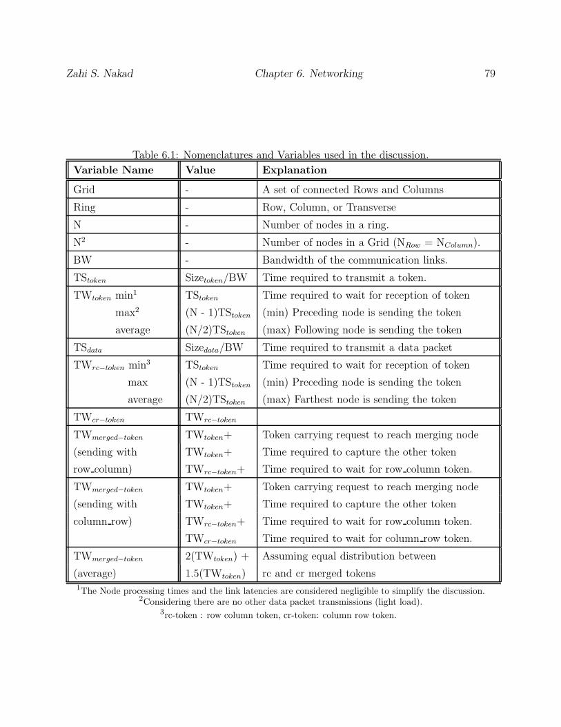
can affect the operation of the network. The values in Table 6.2 and Table 6.3, Section 6.4,
show that communication inside the same ring is the fastest. The number of nodes in a ring
directly affects TWtoken (time to wait for a token) and thus controls the total waiting time
and the number of hops each communication has to experience. The number of nodes in each
ring also dictates the number of grids. Communication on transverse links (between grids)
is more expensive and thus should be minimized. The boundaries between grids should be
chosen considering the communication needs of the application.
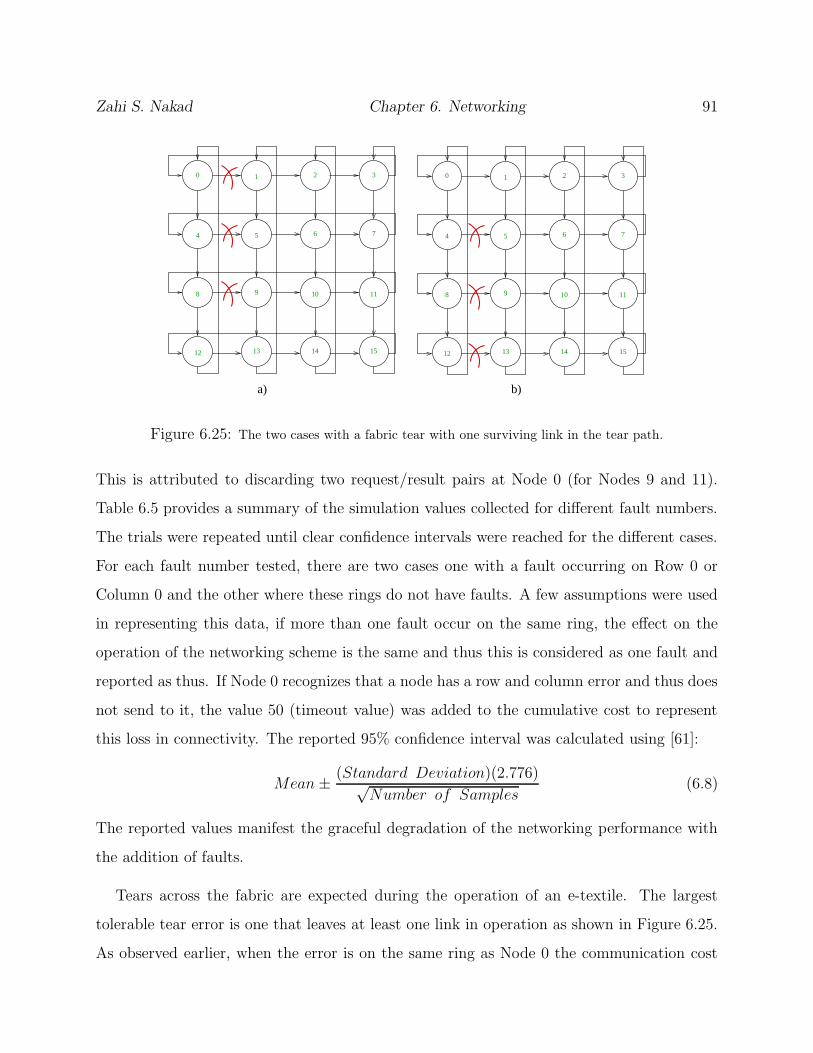
In the presence of faults, a tear across the width of a fabric will totally sever the connection
Zahi S. Nakad Chapter 6. Networking 64
0 1 2 3
5 6 7
10 11
13 14 15
8
4
9
12
RegularNode
Merged Node Route
Wrong
0 1 2 3
5 6 7
10 11
13 14 15
8
4
9
12
GRID 0 GRID 1
Figure 6.5: Node 2 of Grid 1 uses its row ring to forward the data packet to another transverse ring to
reach Grid 0.
between the two parts, thus creating an almost useless grid. The larger the number of nodes
in this grid the more significant the loss of nodes in the overall prototype. As a qualitative
view, the number of nodes in a ring should be small enough to keep the communication
speed-up and reduce the losses when a large tear occurs. The increase in communication
cost across transverse links requires the use of enough nodes inside rings to span enough
area to minimize the need for transverse connections. These views provide guidelines into
deciding the sizes of separate grids. In wearable systems, the flexibility of choosing the grid
size is constrained by the fabric swatches determined by the design of the garment.
6.2 Fault Tolerant Implementation
The implementation of a fault tolerant communication scheme is a must for electronic textiles
systems. The following section discusses the fault tolerant scheme used in this architecture.
Detection of errors and propagating information about the faults are the first aspects pre-
Zahi S. Nakad Chapter 6. Networking 65
0 1 2 3
Figure 6.6: Node 1 has an error at the link directly to its “left.”
sented. Utilization of this information in routing data is then discussed.
6.2.1 Creation of Error packets
The implemented fault tolerant scheme, discussed in detail in Section 6.2.2, requires that the
nodes in the system update error information about the network. The detection of errors
and the transmission of this information will be detailed in this section.
Error detection
Each node is connected to three different rings (row, column, and transverse). There are
three possibilities for link errors. In the case that there are no data packets to be sent on any
link, the nodes will forward the tokens. Each node will keep three separate Timeout Counters
pertaining to each link it is connected to. These counters are reset to zero at the reception
of any data (tokens, data packets, and error packets). If any of these counters reaches a
pre-specified value an error is declared. This value will be dependent on the application and
the specific topology; in this research it is set empirically. When an error is detected in this
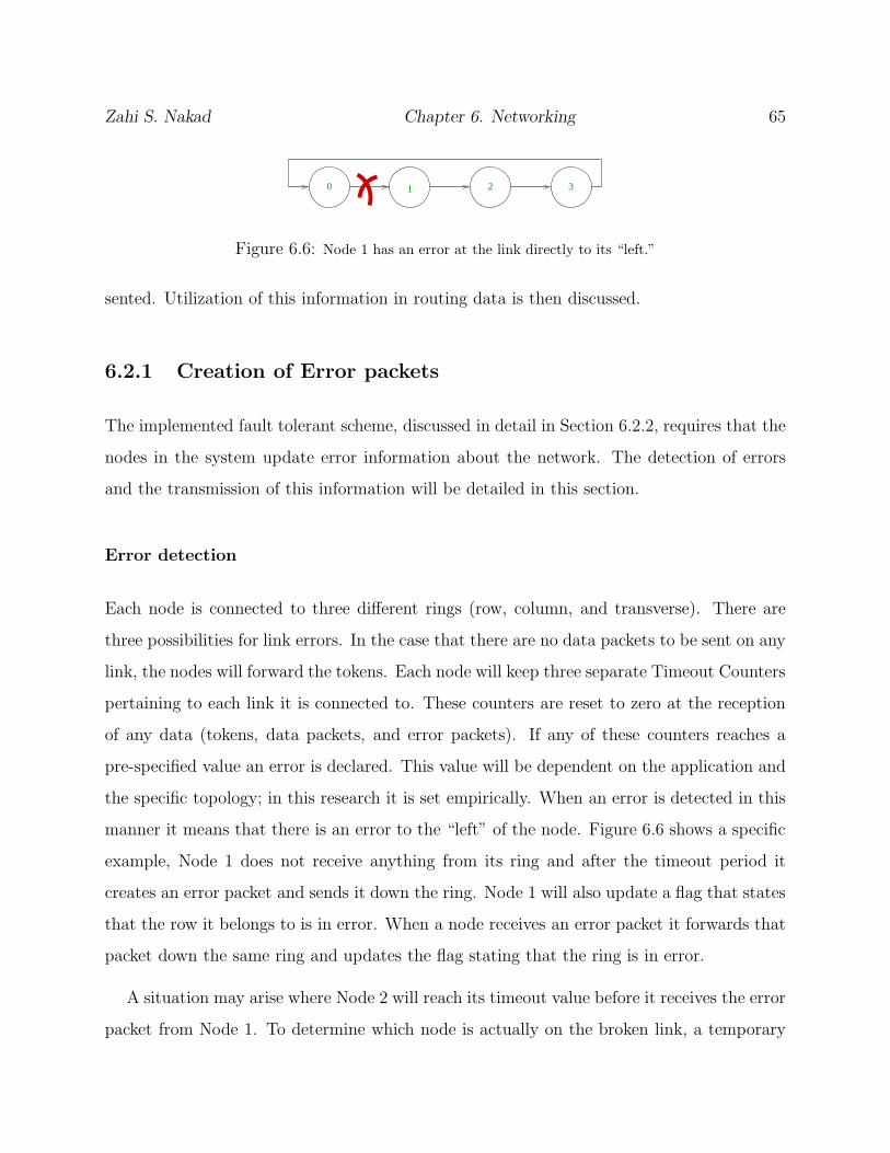
manner it means that there is an error to the “left” of the node. Figure 6.6 shows a specific
example, Node 1 does not receive anything from its ring and after the timeout period it
creates an error packet and sends it down the ring. Node 1 will also update a flag that states
that the row it belongs to is in error. When a node receives an error packet it forwards that
packet down the same ring and updates the flag stating that the ring is in error.
A situation may arise where Node 2 will reach its timeout value before it receives the error
packet from Node 1. To determine which node is actually on the broken link, a temporary
Zahi S. Nakad Chapter 6. Networking 66
0 1 2 3
Figure 6.7: Node 1 and Node 3 have errors at the links directly to their “left.”
error flag is used. When a node first reaches its timeout counter it sends the error packet
and sets the temporary error flag. The error flag is not set unless the timeout period is
reached while the temporary error flag is asserted. Following Figure 6.6, Node 2 will receive
an error packet from Node 1 after it sends its own. This reception will reset the temporary
error flag and thus Node 2 knows that there is an error on the ring and that error is on the
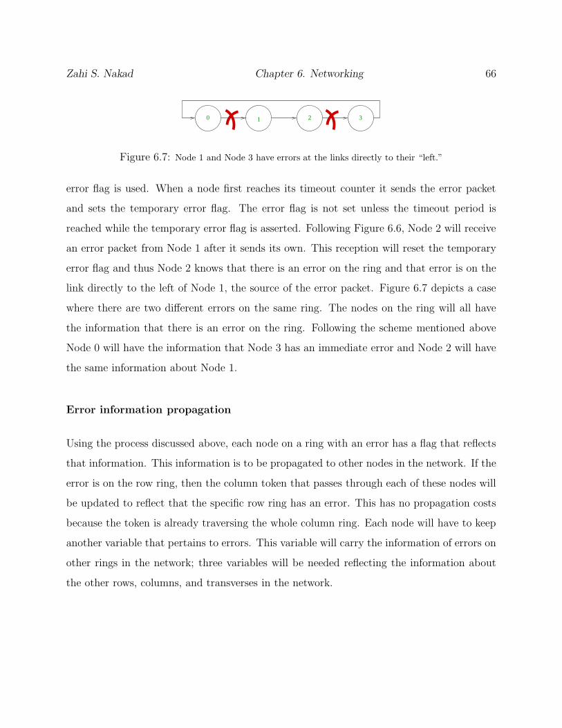
link directly to the left of Node 1, the source of the error packet. Figure 6.7 depicts a case
where there are two different errors on the same ring. The nodes on the ring will all have
the information that there is an error on the ring. Following the scheme mentioned above
Node 0 will have the information that Node 3 has an immediate error and Node 2 will have
the same information about Node 1.
Error information propagation
Using the process discussed above, each node on a ring with an error has a flag that reflects
that information. This information is to be propagated to other nodes in the network. If the
error is on the row ring, then the column token that passes through each of these nodes will
be updated to reflect that the specific row ring has an error. This has no propagation costs
because the token is already traversing the whole column ring. Each node will have to keep
another variable that pertains to errors. This variable will carry the information of errors on
other rings in the network; three variables will be needed reflecting the information about
the other rows, columns, and transverses in the network.
Zahi S. Nakad Chapter 6. Networking 67
0 1 2 3
5 6 7
10 11
13 14 15
8
4
9
12
0 1 2 3
5 6 7
10 11
13 14 15
8
4
9
12
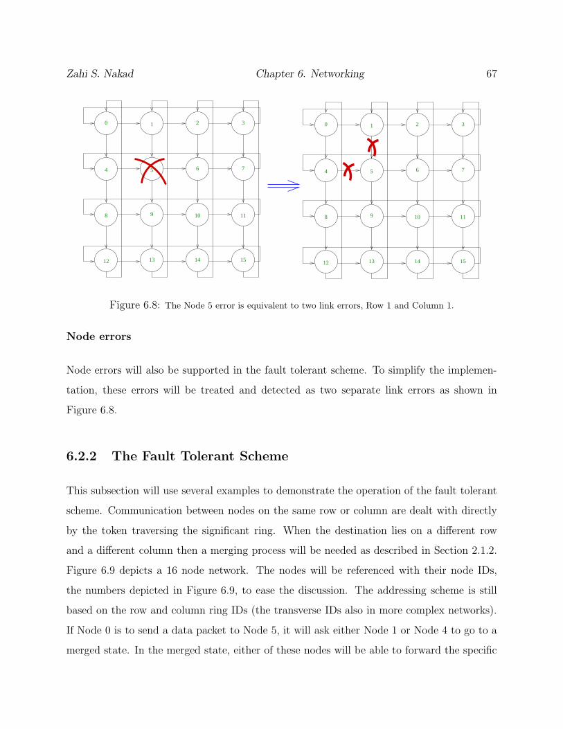
Figure 6.8: The Node 5 error is equivalent to two link errors, Row 1 and Column 1.
Node errors
Node errors will also be supported in the fault tolerant scheme. To simplify the implemen-
tation, these errors will be treated and detected as two separate link errors as shown in
Figure 6.8.
6.2.2 The Fault Tolerant Scheme
This subsection will use several examples to demonstrate the operation of the fault tolerant
scheme. Communication between nodes on the same row or column are dealt with directly
by the token traversing the significant ring. When the destination lies on a different row
and a different column then a merging process will be needed as described in Section 2.1.2.
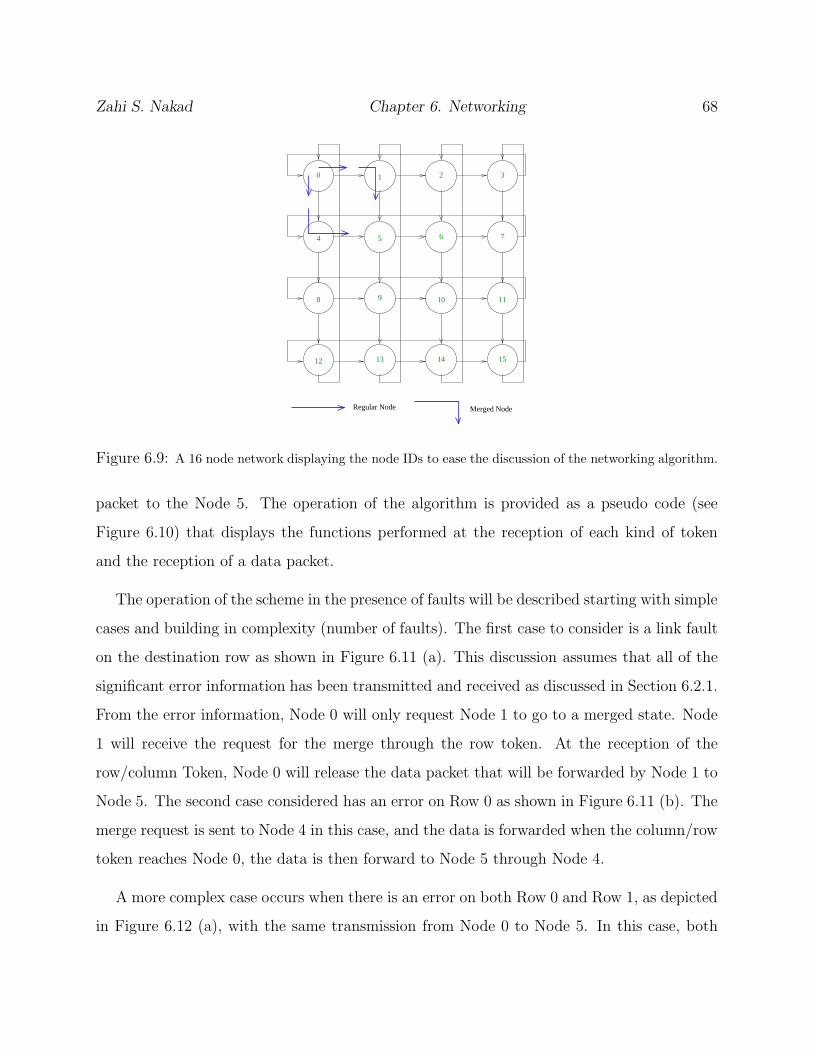
Figure 6.9 depicts a 16 node network. The nodes will be referenced with their node IDs,
the numbers depicted in Figure 6.9, to ease the discussion. The addressing scheme is still
based on the row and column ring IDs (the transverse IDs also in more complex networks).
If Node 0 is to send a data packet to Node 5, it will ask either Node 1 or Node 4 to go to a
merged state. In the merged state, either of these nodes will be able to forward the specific
Zahi S. Nakad Chapter 6. Networking 68
0 1 2 3
5 6 7
10 11
13 14 15
8
4
9
12
Regular Node Merged Node
Figure 6.9: A 16 node network displaying the node IDs to ease the discussion of the networking algorithm.
packet to the Node 5. The operation of the algorithm is provided as a pseudo code (see
Figure 6.10) that displays the functions performed at the reception of each kind of token
and the reception of a data packet.
The operation of the scheme in the presence of faults will be described starting with simple
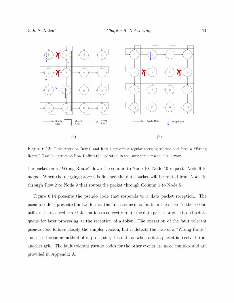
cases and building in complexity (number of faults). The first case to consider is a link fault
on the destination row as shown in Figure 6.11 (a). This discussion assumes that all of the
significant error information has been transmitted and received as discussed in Section 6.2.1.
From the error information, Node 0 will only request Node 1 to go to a merged state. Node
1 will receive the request for the merge through the row token. At the reception of the
row/column Token, Node 0 will release the data packet that will be forwarded by Node 1 to
Node 5. The second case considered has an error on Row 0 as shown in Figure 6.11 (b). The
merge request is sent to Node 4 in this case, and the data is forwarded when the column/row
token reaches Node 0, the data is then forward to Node 5 through Node 4.
A more complex case occurs when there is an error on both Row 0 and Row 1, as depicted
in Figure 6.12 (a), with the same transmission from Node 0 to Node 5. In this case, both
Zahi S. Nakad Chapter 6. Networking 69
- Row Token Arrival:
- if(Data Packet ready for sending):
- If(Destination on same Grid):
- If(Destination on same row): Send data directlyon Row ring.
- else:
- If(Destination on same Column):Column Token will take care of it, no action.
- else: Need a Merger, request onefrom node on the same row as this, and samecolumn as destination. This information is addedto the token that is later released.
- else: Transverse Token will take care of it, no action.
- else: No Action
- If(Waiting For Row Token == 1):
- //Column Token has been captured
- Create a Row Column Token
- Merged Status = 1;
- Waiting For Row Token = 0;
- Send Token on Row ring.
- If(Merged Status == 0):
- If this node was asked to go to a merged state:
- Grab the token
- Waiting For Column Token = 1;
- else: Release the Row Token on the Row ring.
(a)
- Column Token Arrival:
- if(Data Packet ready for sending):
- If(Destination on same Grid):
- If(Destination on same column:) Send data directlyon Column ring.
- else:
- If(Destination on same Row):Row Token will take care of it, no action.
- else: Need a Merger, request onefrom node on the same column as this, and same rowas destination. This information is added to thetoken that is later released.
- else: Transverse Token will take care of it, no action.
- else: No Action
- If(Waiting For Column Token == 1):
- //Row Token has been captured
- Create a Row Column Token
- Merged Status = 1;
- Waiting For Column Token = 0;
- Send Token on Row ring.
- If(Merged Status == 0):
- If this node was asked to go to a merged state:
- Grab the token
- Waiting For Row Token = 1;
- else: Release the Column Token on the Column ring.
(b)
- Row Column Token Arrival:
- if(Data Packet ready for sending):
- If(Destination on same Grid):
- if(Destination Column == Column of Master of Token)&& (This node on a different Row than Destination)
- if this is the master node:
Send data on Column ring.
- else: Send data on Row ring.
- else: Transverse Token will take care of it, no action.
- else: No Action
- if(This is the node that created the Row Column Token)
- Create Column Row Token
- Send Token on Column ring.
- else: Release the Row Column on Row ring.
(c)
- Column Row Token Arrival:
- if(Data Packet ready for sending):
If(Destination on same Grid):
- if(Destination Row == Row of Master of Token)&& (This node on a different Column than Destination)
- if this is the master node:Send data on Row ring.
- else: Send data on Column ring.
else: Transverse Token will take care of it, no action.
- else: No Action
- if(This is the node that created the Column Row Token)
- //The Merged tokens have finished traversing the merged ring.
- Create Row Token and send it on Row ring.
- Create Column Token and send it on Column ring.
- else: Release the Column Row on Column ring.
(d)
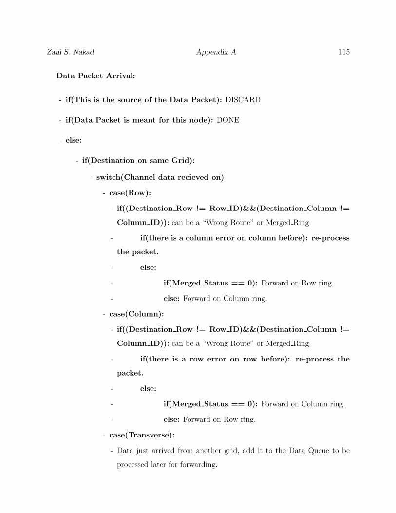
- Data Packet Arrival:
- if(Data Packet is meant for this node): DONE
- else:
- if(Destination on same Grid):
- switch(Channel data recieved on)
- case(Row): if(Merged Status == 0): Forward on Row. Else: Forward on Column.
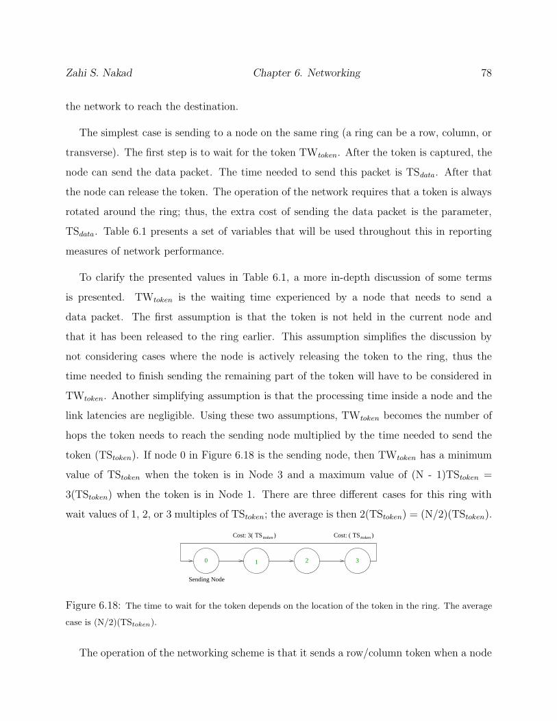
TStoken Send token.1The value of TWtoken assumes no data transmissions from other nodes on the ring.
2The cost to the node here is less than the cost to send the packet. The packet will have to be re-routedonce it reaches the other Grid (adding that cost to the receiving node).
3If the node is on the wrong Transverse ring, then forward on the Row ring until it reaches the correct link.The cost to this node is the same.
first merges. This token traverses the row ring allowing nodes sending to the merged column
to send. When the merged node receives this token, it releases a column/row token on the
column ring to allow nodes on the column to send on the row ring. This provides a smaller
waiting time for a node sending from the row to the column and that is reflected in Table 6.1.
Table 6.2 provides the costs of communication as perceived by the sending node. When
the destination node is on the same ring, the specific location on the ring is not related to
the cost of sending to the source. The source node waits to capture the ring token, sends
the data packet, and then releases the token. This operation is the same if the destination
is the next node in the ring or the farthest. The increase of cost in sending to a farther node
is manifest in the number of hops traversed, this cost is reported in Table 6.3.
In the case of sending to a node on a different grid, the sending node decides to send
Zahi S. Nakad Chapter 6. Networking 81
on either the transverse ring or the row ring. This decision is based on the grids that a
certain transverse ring traverses. If this ring reaches the grid in question, then the data is
forwarded on it, or the data is forwarded on the row ring to reach the other transverse ring.
The assumption here is that the other Transverse Ring will be able to reach the requested
grid. The cost in both cases is the same to the transmitting node, waiting for the needed
token and then sending the data and the token.
This case is totally different when the significant cost is the number of hops in the network.
Assume the node is on the transverse ring that reaches the destination grid. The node has
to capture the transverse token first, and the data is then released on that ring. To reach the
destination grid, the packet has to be forwarded by a node whose transverse link reaches the
other grid. That node is Node 1 on Grid 1 as shown in Figure 6.19, when the communication
is from Grid 1 to Grid 0. If Node 1 is the source of the data, the packet needs to jump one
hop before reaching the other grid, which is the minimum case. If Node 0 is the source, the
first step is 2 jumps or (N/2) jumps. When the packed reaches the new grid, the data is
re-processed for forwarding. The number of hops will then depend on the location of the
final destination.
A last point to investigate is the operation of this networking scheme in a large network,
or the deterioration of the networking performance with an increasing number of nodes in
the network. As mentioned earlier the connection cost includes two costs, the cost to the
sending node and the cost in number of hops to reach the destination. The cost to the
sending node as shown in Table 6.2 depends on TWtoken or TWmerged−token. According to
Table 6.1 TWmerged−token is a function of TWtoken which is dependent on N (the number of
nodes in a ring). The cost to the sending node increases with increasing the number of nodes
in the ring and not the number of nodes in the network. In a square network, this increase
is dependant on√
N2 = N where N 2 is the number of nodes in the network. The cost on
the sending node is not affected in the presence of a transverse connection because in both
cases the node waits for TWtoken before sending.
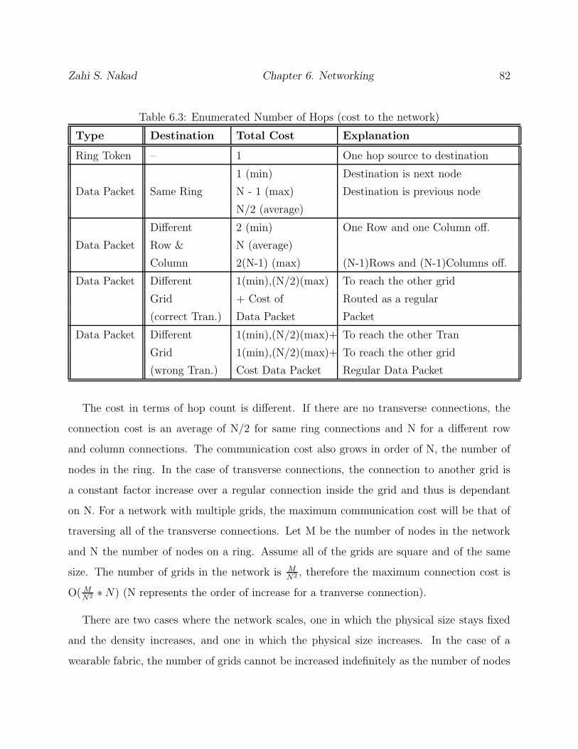
Zahi S. Nakad Chapter 6. Networking 82
Table 6.3: Enumerated Number of Hops (cost to the network)
Type Destination Total Cost Explanation
Ring Token – 1 One hop source to destination
1 (min) Destination is next node
Data Packet Same Ring N - 1 (max) Destination is previous node
N/2 (average)
Different 2 (min) One Row and one Column off.
Data Packet Row & N (average)
Column 2(N-1) (max) (N-1)Rows and (N-1)Columns off.
Data Packet Different 1(min),(N/2)(max) To reach the other grid
Grid + Cost of Routed as a regular
(correct Tran.) Data Packet Packet
Data Packet Different 1(min),(N/2)(max)+ To reach the other Tran
Grid 1(min),(N/2)(max)+ To reach the other grid
(wrong Tran.) Cost Data Packet Regular Data Packet
The cost in terms of hop count is different. If there are no transverse connections, the
connection cost is an average of N/2 for same ring connections and N for a different row
and column connections. The communication cost also grows in order of N, the number of
nodes in the ring. In the case of transverse connections, the connection to another grid is
a constant factor increase over a regular connection inside the grid and thus is dependant
on N. For a network with multiple grids, the maximum communication cost will be that of
traversing all of the transverse connections. Let M be the number of nodes in the network
and N the number of nodes on a ring. Assume all of the grids are square and of the same
size. The number of grids in the network is MN2 , therefore the maximum connection cost is
O( MN2 ∗ N) (N represents the order of increase for a tranverse connection).
There are two cases where the network scales, one in which the physical size stays fixed
and the density increases, and one in which the physical size increases. In the case of a
wearable fabric, the number of grids cannot be increased indefinitely as the number of nodes
Zahi S. Nakad Chapter 6. Networking 83
is increased. In this case the factor MN2 is O(1) and the overall communication cost is O(N).
In a large-scale application the number of grids in the network increases with the number of
nodes and thus the communication cost is O( MN2 ∗ N) = O(M/N).
0 1 2 3
GRID 0 GRID 1
0 1 2 3
Figure 6.19: Communication costs (number of hops) varies greatly when the data packet transverses two
grids.
6.4.1 Transmission Costs in the Presence of Errors
There is almost always an increase in the cost of transmission in the presence of faults.
This increase in cost is more dramatic in the number of hops measure. The two measures
introduced in the previous section will be used to measure the cost of communication between
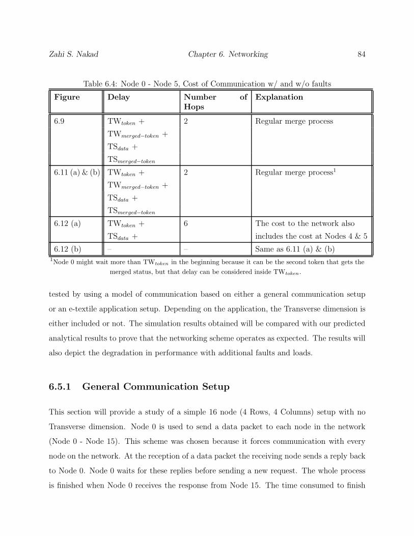
Node 0 and Node 5 in the scenarios provided in Figures 6.9-6.12. Table 6.4 reports these
numbers.
The cost of communication varies with the location of the fault and the specific com-
munication path under study. A more quantitative study will be provided in Section 6.5.
Specific communication sequences will be provided with the effects of the faults. The next
section will provide two approaches to studying the network behavior, an analytical method
to predict the general response of the network and a simulation approach to describe the
complex behaviors.
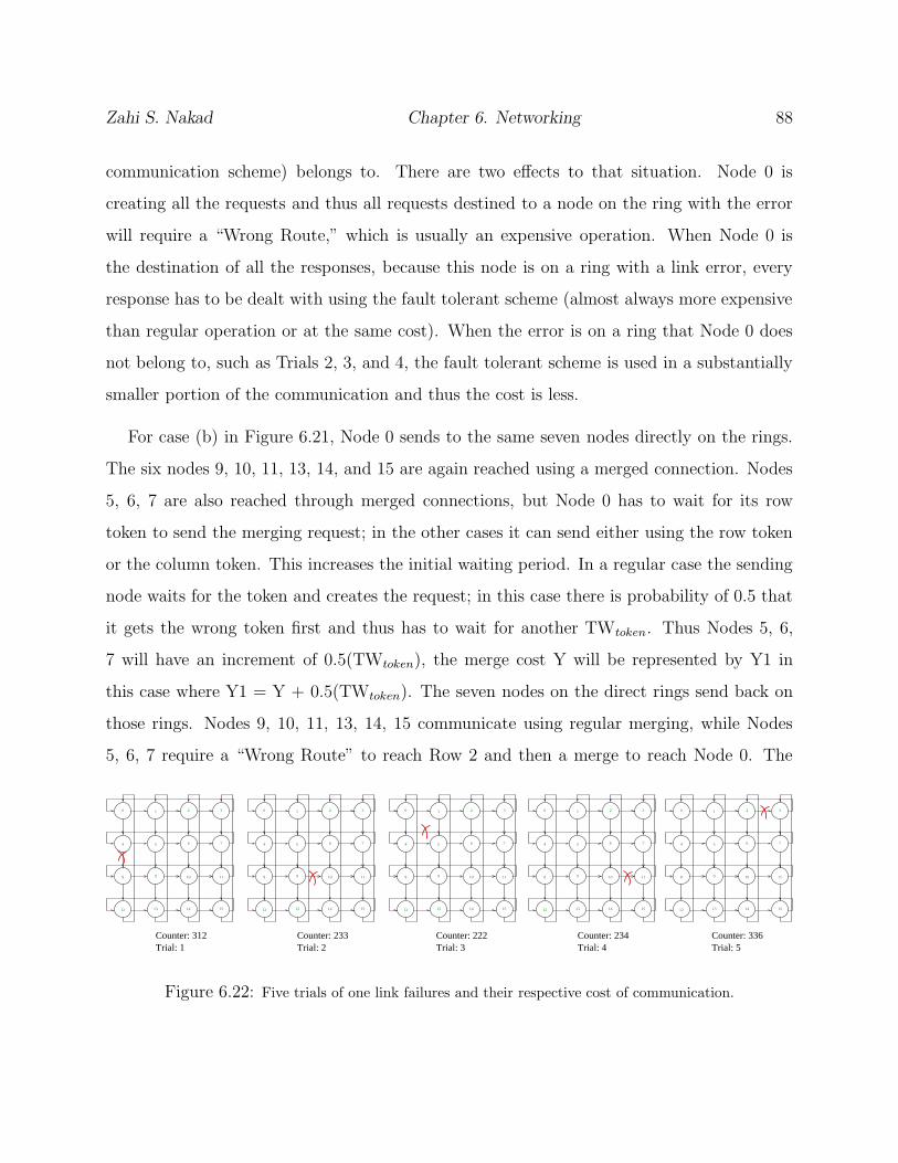
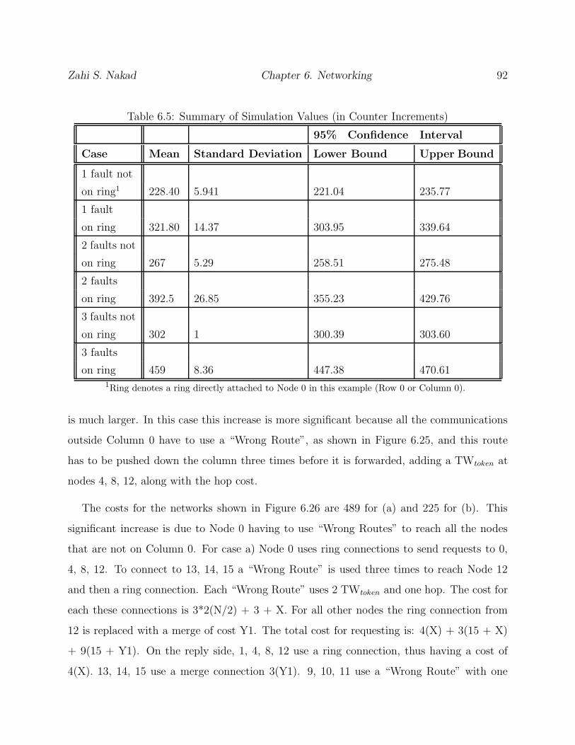
6.5 Results
The following section presents the results collected from simulating the networking scheme
under varying fault occurrences, loads, and sleeping nodes. The networking scheme was
Zahi S. Nakad Chapter 6. Networking 84
Table 6.4: Node 0 - Node 5, Cost of Communication w/ and w/o faults
Figure Delay Number ofHops
Explanation
6.9 TWtoken + 2 Regular merge process
TWmerged−token +
TSdata +
TSmerged−token
6.11 (a) & (b) TWtoken + 2 Regular merge process1
TWmerged−token +
TSdata +
TSmerged−token
6.12 (a) TWtoken + 6 The cost to the network also
TSdata + includes the cost at Nodes 4 & 5
6.12 (b) – – Same as 6.11 (a) & (b)1Node 0 might wait more than TWtoken in the beginning because it can be the second token that gets the
merged status, but that delay can be considered inside TWtoken.
tested by using a model of communication based on either a general communication setup
or an e-textile application setup. Depending on the application, the Transverse dimension is
either included or not. The simulation results obtained will be compared with our predicted
analytical results to prove that the networking scheme operates as expected. The results will
also depict the degradation in performance with additional faults and loads.
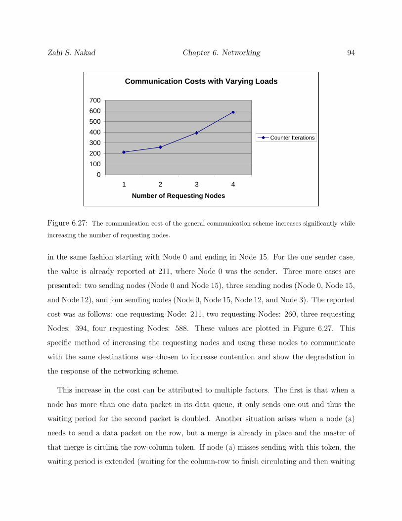
6.5.1 General Communication Setup
This section will provide a study of a simple 16 node (4 Rows, 4 Columns) setup with no
Transverse dimension. Node 0 is used to send a data packet to each node in the network
(Node 0 - Node 15). This scheme was chosen because it forces communication with every
node on the network. At the reception of a data packet the receiving node sends a reply back
to Node 0. Node 0 waits for these replies before sending a new request. The whole process
is finished when Node 0 receives the response from Node 15. The time consumed to finish
Zahi S. Nakad Chapter 6. Networking 85
0 1 2 3
5 6 7
10 11
13 14 15
8
4
9
12
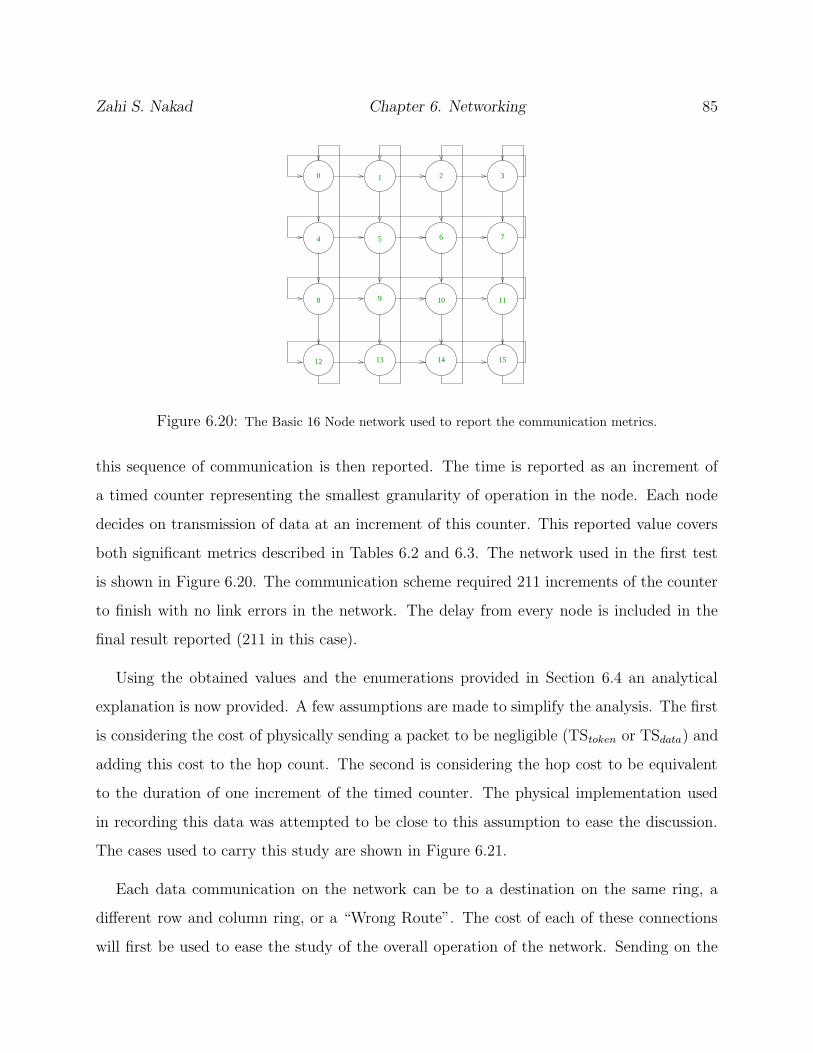
Figure 6.20: The Basic 16 Node network used to report the communication metrics.
this sequence of communication is then reported. The time is reported as an increment of
a timed counter representing the smallest granularity of operation in the node. Each node
decides on transmission of data at an increment of this counter. This reported value covers
both significant metrics described in Tables 6.2 and 6.3. The network used in the first test
is shown in Figure 6.20. The communication scheme required 211 increments of the counter
to finish with no link errors in the network. The delay from every node is included in the
final result reported (211 in this case).
Using the obtained values and the enumerations provided in Section 6.4 an analytical
explanation is now provided. A few assumptions are made to simplify the analysis. The first
is considering the cost of physically sending a packet to be negligible (TStoken or TSdata) and
adding this cost to the hop count. The second is considering the hop cost to be equivalent
to the duration of one increment of the timed counter. The physical implementation used
in recording this data was attempted to be close to this assumption to ease the discussion.
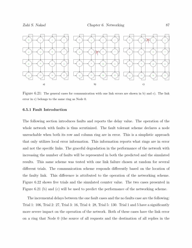
The cases used to carry this study are shown in Figure 6.21.
Each data communication on the network can be to a destination on the same ring, a
different row and column ring, or a “Wrong Route”. The cost of each of these connections
will first be used to ease the study of the overall operation of the network. Sending on the
Zahi S. Nakad Chapter 6. Networking 86
same ring requires a TWtoken according to Table 6.2 and an average of N/2 hops according
to Table 6.3, where N is the number of nodes in the ring. The cost in overall time to send
a data packet on the ring is then (TWtoken + (N/2)) counter iterations. Using the stated
assumption that TWtoken = (N/2), considering the cost to send the token and the hop itself
equivalent to a counter iteration, the cost of sending on the ring (X) in this case is:
X =N
2+
N
2= N = 4 (6.1)
Sending a data packet to a destination on a different row and column requires the use of a
merge. The sending Node has to wait for TWmerged−token and the connection will require N
hops on average. The cost of sending with a merge (Y) is:
Y = TWmerged−token + N = 3.5(TWtoken) + N = 3.5 ∗ (N
2) + N = 11 (6.2)
The last communication type to consider is the “Wrong Route,” which occurs in some of
the cases with faults in the network. In the cases considered for the study, shown in Fig-
ure 6.21 (b) and (c) the “Wrong Route” forces the packets on rings that require a merge
to reach the final destination. The “Wrong Route” forces an additional TWtoken to wait for
the token in the forced direction, then one hop to the corresponding ring, another TWtoken
awaiting the processing at the data queue and finally a merged communication. The total
cost of the connection (W) is (where Y1 is the merge cost, which will be explained in the
next paragraph):
W = 2(TWtoken) + 1(hop) + Y 1 = 2(N
2) + 1 + Y 1 = 5 + Y 1 (6.3)
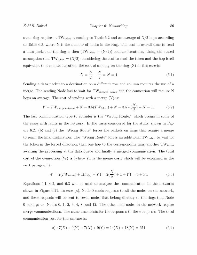
Equations 6.1, 6.2, and 6.3 will be used to analyze the communication in the networks
shown in Figure 6.21. In case (a), Node 0 sends requests to all the nodes on the network,
and these requests will be sent to seven nodes that belong directly to the rings that Node
0 belongs to: Nodes 0, 1, 2, 3, 4, 8, and 12. The other nine nodes in the network require
merge communications. The same case exists for the responses to these requests. The total