92


ARCHIVES OF CIVIL AND MECHANICAL ENGINEERING
Vol. IV 2004 No. 4
Cross-current lamella sedimentation tanks
WŁODZIMIERZ P. KOWALSKI, RAFAŁ MIĘSOUniversity of Mining and Metallurgy, Al. Mickiewicza 30, Kraków
The paper outlines the design of sedimentation tanks and installations utilising the Boycott’s effect. Three major types of configuration of lamella installations are presented: counter-current, cross-current and parallel flow. Cross-current sedimentation is thoroughly investigated and simulations that use thus obtained results are summarised. The results of the experimental program and of simulations reveal that the capacity of cross-current lamella tanks can be increased tenfold or sedimentation efficiency can be vastly improved. Accordingly, a computer-assisted design of a cross-current tank with the capacity of 100 m3/h is made. Such an installation will be most useful in high-efficiency clarification of suspensions from industrial processes or from water purification and waste treatment systems.
Keywords: cross-current sedimentation, lamella packs, settling tanks, water clarification
Nomenclature ρ, ρ0 – density of solid phase and of liquid phase, respectively, µ 0 – dynamic viscosity, pw – specific surface of the lamella packet, F, F1, F2 – settling surface areas, Q – suspension flow rate, q – surface loading, overflow rate, d – equivalent particle size (diameter), dg – critical grain size, v, vg – settling velocities of particles of the size d, dg, respectively, f (d ) – probability function of grain diameter, f (v) – probability function of settling velocity, Φ (a) – distribution function in the log-normal distribution N (0.1), Φ –1(a) – fractile of the normal distribution N (0.1), m, σ – parameters of the log-normal distribution of particles size, Γ (a) – Euler’s gamma function, Γ (a, b) – incomplete gamma function, d0, p, n – parameters in the generalised gamma distribution of the particles size (scale pa-
rameter, shape parameters), η – sedimentation efficiency.
1. Introduction
Lamella tanks are now in widespread use in water and wastewater treatment in-stallations. They belong to a group of sedimentation tanks whose running costs are relatively low, and investment costs – quite high. That refers particularly to conven-
W. P. KOWALSKI, R. MIĘSO 6
tional rectangularly shaped or round Dorr clarifiers. When the running costs are on a low level, it is possible to vastly reduce the investment costs.
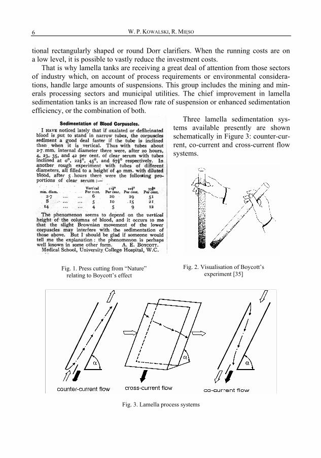
That is why lamella tanks are receiving a great deal of attention from those sectors of industry which, on account of process requirements or environmental considera-tions, handle large amounts of suspensions. This group includes the mining and min-erals processing sectors and municipal utilities. The chief improvement in lamella sedimentation tanks is an increased flow rate of suspension or enhanced sedimentation efficiency, or the combination of both.
Three lamella sedimentation sys-tems available presently are shown schematically in Figure 3: counter-cur-rent, co-current and cross-current flow systems.
Fig. 3. Lamella process
Fig. 2. Visualisation of Boycott’s experiment [35]
Fig. 1. Press cutting from “Nature”relating to Boycott’s effect
systems

Cross-current lamella sedimentation tanks
7
The counter-current system, where the suspension flows in the direction opposite to that of the sliding particles, is now most widely applied. Sedimentation proceeds in conduits made of corrugated plates. A lamella packet of the envised type, manufac-tured in Poland, is shown in Figure 4. The lamella packet performance depends on the relative length of conduits. Engineering the tubes with the relative length over 10 is quite a difficult task.
The cross-current flow system comes next in the ranking list. In the cross-current configuration, the suspension flows horizontally and the sediment flows along the in-clined plates in the direction normal to that of the suspension movement. This ar-rangement seems to be most attractive because, unlike the counter-current systems, an increase in the settling surface is not restricted by design data.
Fig. 4. Lamella packet of the envised type
Fig. 5. Diagram of the SERPAC tank

W. P. KOWALSKI, R. MIĘSO 8
Figures 5 and 6 show counter-current packets used to modernise the existing rec-tangularly shaped tanks [9].
Fig. 6. Application of counter-current lamella packets in an existing tank [9]
The parallel flow system, where the suspension flows downwards in the same di-rection as the settling particles, seems the least popular and its applications are but a few because the clarified suspension and thickened sediment will mix while leaving the sedimentation area. Nonetheless, a parallel flow system works really well as a sludge thickener.
2. Investigations of cross-current sedimentation processes
Cross-current lamella systems have been extensively studied in several research centres [12, 24], the main objective being to find out how lamella packet surface and configuration should affect sedimentation efficiency and tank performance.
2.1. Experimental set-up
A new original experimental stand at the AGH (University of Science and Technol-ogy) allows full-scale investigations of cross-current lamella processes. Results of the experimental programme were used to formulate the guidelines for the design of an industrial tank with the capacity of 100 m3/h. The computer model of the tank is also developed. The experimental set-up has two main elements (see Figure 5):

Cross-current lamella sedimentation tanks
9
1. Rectangularly shaped tank with cross-current lamellas, consisting of a feed sup-ply chamber, an overflow collector, an underflow collector or, alternatively, small sediment collectors.
2. Support structure.
Fig. 7. Experimental set-up: sedimentation tank and a supporting structure
Fig. 8. Feed supply/flooding chamber and a portion of lamella packets
The model of a cross-current sedimentation tank is made of organic glass plates (5 mm thick) and has three major components: a feed supply chamber, a sedimentation chamber and an overflow chamber.
Fig. 9. Tube supplying the feed in a horizontal configuration
Fig. 10. Movable plate ensuring a uniform distribution of the suspension
The feed supply chamber (Figure 7) 100 × 100 × 500 mm is provided with a perfo-rated dosing tube (Figure 9) connected to a dosing valve (ball valve ¾” ) mounted in a cover.

W. P. KOWALSKI, R. MIĘSO 10
Fig. 11. Sediment collector Fig.12. Hoppers for sediment collection
The valve is screwed indirectly in the chamber cover. The precise finish of the cover edge ensures that the dosing tube coincides with the chamber axis. The holes in the dosing tube open to the sidewalls and the wall opposite to the sedimentation chamber. At the bottom the tube is secured with a cork which prevents the feed flow into the supply chamber as well as mixing and drifting of sediment collected in the first settling tray (Figure 9). Hence the mass of sediment retained in the supply cham-ber can be precisely established.
The supply chamber is separated from the sedimentation chamber by a removable corrugated panel (Figure 12).
Fig. 13. Cross-current lamella packets in the sedimentation
chamber
Fig. 14. A plate distributing the suspension – general view
Fig. 15. Overflow-collecting pipe

Cross-current lamella sedimentation tanks
11
The corrugations on the dosing tube and the separating panel aimed at stabilising the feed flow in the sedimentation chamber. The sedimentation chamber (Figure 5) is equipped with a settling system and two suspended collecting hoppers with discharge valves (ball valves ½”) (Figure 10).
On the skeleton structure hatches appear which seem to be an securing the sup-porting plates inclined at 55°. Six such plates are mounted in that position (Figure 11). Supporting plates are made of organic glass, 1.5 mm thick.
Sediment is collected by two hoppers dividing the tank bottom into two equal parts. Hoppers have bolted ball valves ½”. The design of the sedimentation chamber allows mounting settling trays over the hoppers, these trays dividing the sedimentation chamber into five equal settling zones. Sediment collected in trays can be subjected to quantitative analysis as well as grain size distribution analysis. When no settling trays are provided, the sedimentation chamber is equipped with an openwork insert which can be fixed in the same position. The insert is made of organic glass rods of rectan-gular cross-section. The sedimentation chamber is separated from the overflow cham-ber by a thin panel wall made of organic glass, 5 mm thick.
Fig. 16. Experimental set-up: 1–feed tank, 2–mixer drive, 3–outflow from the feed tank, 4–peristaltic pumps, 5–conduits transporting the suspension, 6–cross-current lamella packets, 7–feed inflow to the
settling tank model, 9–overflow collector, 10–cross-current flow tank model

W. P. KOWALSKI, R. MIĘSO 12
The overflow chamber is 100 mm in width, 100 mm in length and 500 mm in height. Half-way up the chamber is a discharge ball valve ¾” (Figure 13). The thread is cut in the organic glass cube, glued to the chamber wall and sealed with a silicone band.
The whole tank is made of transparent materials enabling easy and full monitoring of sedimentation processes. Ball valves ensure smooth regulation and fast control of flow rate. The glue Acrifix 116, intended for organic glass exclusively, provides dura-ble, fast holding and tight proof connection as long as the gluing procedure is pursued in the prescribed manner.
The settling tank is mounted on the supporting structure made from stainless steel. The upper section of the frame is made of rods with rectangular cross-section and the lower part is made of a flat bar and two plates to mount the supply and overflow chambers. The settling chamber is positioned between the two flat bars. Half-way along, on the spot where collecting hoppers are connected, there is a bracket support-ing the settling tank and making the load-bearing structure more rigid. Bushings fixing the supports are welded to each of the plates. The lower parts of the supports are mounted in footings made of steel St3Sx coated with an epoxy dye and a surface var-nish, as corrosion control measures. The supports are made of stainless pipes.
In accordance with the design objectives, the structural elements are easy to as-semble and disassemble. Most elements of the stand are secured with set screws. The openwork construction allows full monitoring of sedimentation processes.
The experimental set-up shown schematically in Figure 16 includes: a feed tank, a mixer arm, peristaltic pumps, conduits transporting the suspension, cross-current la-mella packets, collectors of thickened sediment, the model of a cross-current tank.
2.2. Results
The main objective of the tests was to explore how to modernise the clarification system in a battery recycling installation. The two-stage clarification process was de-signed: in a Dorr clarifier and in a cross-current lamella tank. The sample analyses were collected accordingly.
Representative results are shown in Figure 17.
Fov
ig. 17. Sedimentation efficiency versus erflow rate in cross-current sedimentation
Cross-current lamella sedimentation tanks
13
The solid phase content in the feed material ranges from 40 kg/m3 to over 120 kg/m3. The solid phase content in the overflow falls between 0.800 kg/m3 and 0.120 kg/m3. These results are consistent with our predictions. The effects of modernisation can therefore be regarded as satisfactory. However, it is anticipated that solid phase content in water treated in a Dorr clarifier might be exceeded in the future and that is why the two-stage clarification is provided. The second-stage clarification proceeds in a cross-current lamella tank.
2.3. Mathematical model of cross-current sedimentation
The starting point is Hazen’s theory of sedimentation and its generalisations sug-gested by Kowalski [20, 21], who has demonstrated that Hazen’s sedimentation theory applies just as well to tanks with an inclined bottom [16] and that idealisation of sus-pension flow in elementary lamella conduits is responsible for slight undervaluing cal-culation results, at the same time the calculations become easier and less cumbersome. Taking into account the specialists’ opinions [1–7, 26, 35], results of tests, calculations and computer simulations, the authors provide below an algorithm based on the works quoted above.
An assumption is made that the whole surface available in a sedimentation tank is a major determinant of the process efficiency. When the tank is not filled with lamella packets, the settling surface is taken as equal to the design value, in other words it equals the surface of the water table. In a tank filled with lamella packets, two settling surfaces are distinguished: that without and that with lamella packets (F1 and F2, re-spectively). The surface F2 contained in the packet conduits is obtained as the product of the surface occupied by the packet layer and the specific surface factor ph. The spe-cific surface factor ph is determined on the basis of design parameters of the lamella packet and complex features of suspension flow (developing laminar flow, well devel-oped laminar flow or flow with the rectangularly shaped velocity distribution pattern). The specific surface factor ph indicates how many times the settling surface available in a lamella packet is greater than the surface occupied by the packet. It was shown in [17] that surface areas F1 and F2 are additive as long as certain assumptions are made. For convenience the sum F1 + F2 is used in further calculations as the available settling surface. Knowing the suspension flow rate Q, we obtain the surface load q equal to the settling velocity of critical grains in the given process conditions:
).(21
gdvFQ
FFQq =+
= (1)
The settling velocity v(dg) of critical grains is derived on the basis of the analysis of particles’ flow in liquids (governed by Stokes formula), where ρ and ρ0 stand for solid phase and liquid phase density, respectively, µ0 is dynamic viscosity and g is accel-eration of gravity:

W. P. KOWALSKI, R. MIĘSO 14
.)(181)( 2
0
0gg dgdv
µρρ −
= (2)
Formula (2) yields the critical grain size dg. Knowing the type of statistical distri-bution of solid phase grain size f(d ) and the distribution parameters obtained from grain-size measurements, we obtain the sedimentation efficiency η :
.)()(10 0
2∫ ∫+−=g gd d
dddfddddfη (3)
The actual formulation of (3) depends on the type of solid phase particle-size dis-tribution f (d ). For some specific cases analytical solutions [22] are provided. When the grain-size distribution f (d ) follows the log-normal pattern with the density func-tion of the parameters m and σ (the mean value and standard deviation of the distribu-tion of grain-size natural logarithms)
,ln21exp
π21),;(
2
⎟⎟⎠
⎞⎜⎜⎝
⎛⎟⎠⎞
⎜⎝⎛ −
−=σσ
σ mdd
mdf (4)
then for the argument a the analytical form of (3) related to the distribution function ΦN(a) holds:
.2ln
)](ln[2exp
ln1),;(
2⎟⎟⎠
⎞⎜⎜⎝
⎛⋅−
−⋅−−⋅+
⎟⎟⎠
⎞⎜⎜⎝
⎛ −−=
σσ
σ
σση
mdΦmd
mdΦmd
gNg
gNg
(
When the solid phase particle-size distribution f(d) follows the generalised gammdistribution with the density function of the parameters d0, n, p (scale parameter ashape parameters):
,exp)(
),,;(0
1
000
⎥⎥⎦
⎤
⎢⎢⎣
⎡⎟⎟⎠
⎞⎜⎜⎝
⎛−⋅⎟⎟
⎠
⎞⎜⎜⎝
⎛=
− npn
dd
dd
pΓdnnpddf (
Equation (3) is rewritten as:
5)
a nd
6)

Cross-current lamella sedimentation tanks
15
.)(
,2
)(
,
1),,;(0
2
000 pΓ
dd
npΓ
dd
pΓ
dd
pΓ
npdd
ng
g
ng
g
⎥⎥⎦
⎤
⎢⎢⎣
⎡⎟⎟⎠
⎞⎜⎜⎝
⎛+
⋅⎟⎟⎠
⎞⎜⎜⎝
⎛+
⎥⎥⎦
⎤
⎢⎢⎣
⎡⎟⎟⎠
⎞⎜⎜⎝
⎛
−=η (7)
Γ (a) is a well-known Euler’s gamma function and Γ (a, b) is the incomplete Euler’s gamma function:
.)(
1),(0
1∫ −− ⋅=b
ta dtexaΓ
baΓ (8)
With reference to (8) we write:
,2npapa +== or .
0
ng
dd
b ⎟⎟⎠
⎞⎜⎜⎝
⎛= (9)
In order to compute the sedimentation efficiency from (5) or (7), we ought to know the parameters of the grain-size distribution and the critical grain size dg. Parameters of the statistical distribution of the solid phase particle size are obtained from granu-lometric analysis [18, 19].
Theoretical considerations of computations of sedimentation efficiency of polydis-persive suspensions seem rather complicated though the available computer tech-niques render the task feasible. All the same, the model can be simplified by assuming one of the boundary velocity distributions, so as to have it developed laminarly or rectangularly shaped. The calculation procedure becomes less complicated, though less accurate. According to the authors, this inaccuracy is fully acceptable in the in-vestigations of dilute suspensions.
2.4. Computer simulations
Computer simulations of cross-current sedimentation processes are based on the mathematical model presented above. Simulation procedures involved the calculation of sedimentation efficiency for the assumed tank geometry, physical properties of the suspension and its flow rate.
Geometric parameters of the tank are expressed in terms of the settling area de-pendent on the tank dimensions, the number of plates making up the lamella packet and plate inclination angle. The following parameters of the suspension were consid-ered: solid and liquid phase density, temperature of the suspension expressed in terms of the dynamic viscosity and solid phase grain-size distribution, represented by the distribution pattern of a random variable. For the purpose of simulations, the grain-

W. P. KOWALSKI, R. MIĘSO 16
size distribution is assumed to be log-normal. Suspension flow rate and settling surface (i.e. tank geometry parameters) are ex-
pressed as the surface load factor – the flow rate to settling surface ratio. Having ob-tained the surface loading, solid phase and liquid phase density and dynamic viscosity of the liquid phase, the particle sizes were determined for the given process condi-tions.
Therefore, computer simulations are brought down to the calculation of sedimenta-tion efficiency as the function dependent on surface loading q and enveloping tank ge-ometry, suspension flow rate, physical properties of the suspension (particularly the solid phase density and grain-size distribution given in terms of log-normal parame-ters: m – mean value of natural logarithms of particle size and σ – standard deviation of particle sizes’ natural logarithms).
Formally, the relationship applied in simulations:
),,,,( gdmqf ση = (10)
where
),( gdvFQq ==
(11)
.)(
18
0
0 qg
dg ⋅⋅−
⋅=
ρρµ (12)
The dynamic viscosity is determined from the formula:
,000222.00337.01
1079.12
3
0 t⋅++⋅
=−
µ (13)
where t stands for suspension temperature [°C]. The suspension temperature is as-sumed t = 20 °C and the dynamic viscosity µ0 is equal to 1·10–3 kg/m/s.
Selected results of computer simulations are shown in Figures 19–26. Sedimenta-tion efficiency is plotted as the function of surface loading (in the range of 0–1.5 m3/m2/h) for the specified values of log-normal parameters: m = 2.0, 2.5, 3.0, 3.5 and σ = 0.6, 1.0. In each case, five curves are plotted to show the influence of the solid phase particles density ρ = 2000, 3000, 4000, 5000, 6000 kg/m3.
It is readily apparent that the influence of the surface loading is essential. In the case of suspensions containing the finest solid particles (m = 2, σ = 0.6, see Figure 17) the sedimentation efficiency over 0.8–0.9 is achievable, provided that surface loading

Cross-current lamella sedimentation tanks
17
cannot exceed the value of 0.15 m3/m2/h, no matter what the solid phase density. The influence of the solid phase density is vital when the sedimentation efficiencies achieved turn out to be low. For example, for a surface loading of 1 m3/m2/h the sedi-mentation efficiency of particles with the density of 6000 kg/m3 is 0.6, while for the particles’ density of 2000 kg/m3 it will be slightly more than 0.2.
Fig. 18. Sedimentation efficiency versus surface loading for m = 2.0 and σ = 0.6
Fig. 19. Sedimentation efficiency versus surface loading for m = 2.0 and σ = 1.0
Fig. 20. Sedimentation efficiency versus surface loading for m = 2.5 and σ = 0.6
Fig. 21. Sedimentation efficiency versus surface loading for m = 2.5 and σ = 1.0

W. P. KOWALSKI, R. MIĘSO 18
Results of computer simulations might be used in preliminary evaluation of sedi-
mentation efficiency.
Fig. 22. Sedimentation efficiency versus surface loading for m = 3.0 and σ = 0.6
Fig. 23. Sedimentation efficiency versus surface loading for m = 3.0 and σ = 1.0
Fig. 24. Sedimentation efficiency versus surface loading for m = 3.5 and σ = 0.6
Fig. 25. Sedimentation efficiency versus surface loading for m = 3.5 and σ =1.0
3. Design of a cross-current sedimentation tank
These design guidelines have their relevance to the new prototype of a cross-cur-rent lamella sedimentation tank intended for clarification of suspensions from the first-
Cross-current lamella sedimentation tanks
19
stage treatment process in a Dorr clarifier. The input data for the design are the results of investigations and simulations summarised in the previous chapters.
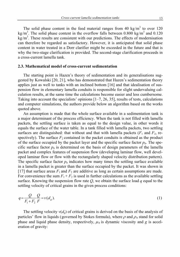
Suspension flowing at the rate of approximately 120 m3/h enters the cross-current tank, about 20 m3/h of the suspension will be discharged via an underflow. Thus we obtain the flow rate of about 100 m3/h of the suspension with the solid phase content nearing zero.
Extensive tests and simulations reveal that surface loading in the tank should not exceed 0.25 m3/m2/h and hence the settling surface should be at least 400 m2. It is sug-gested that two “twin” tanks be built. Application of 25 lamella packet segments is feasible, thereby increasing the settling surface 25-fold in relation to the surface occu-pied by the packets. Let the base of the working unit of one tank have the surface area of 10 m2. The available settling surface will be 250 m2, leaving a safety margin of 20%.
Fig. 26. Model of cross-current sedimentation tank – general view
In the preliminary stage of design, it is assumed that the tank housing will be made of steel, though other options are considered, too. The housing might be also made of plastic materials and that solution offers several benefits: resistance to corrosion and
W. P. KOWALSKI, R. MIĘSO 20
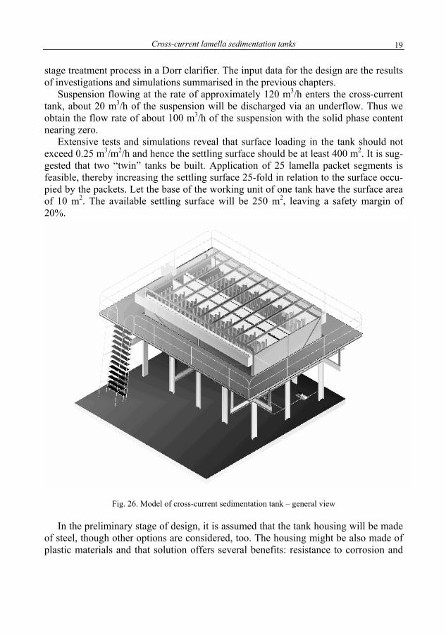
vastly reduced maintenance costs. However, the cost of constructing a plastic frame will be decidedly higher.
Fig. 27. Tank structure without wall, with a single lamella packet
Fig. 28. Model tank interior
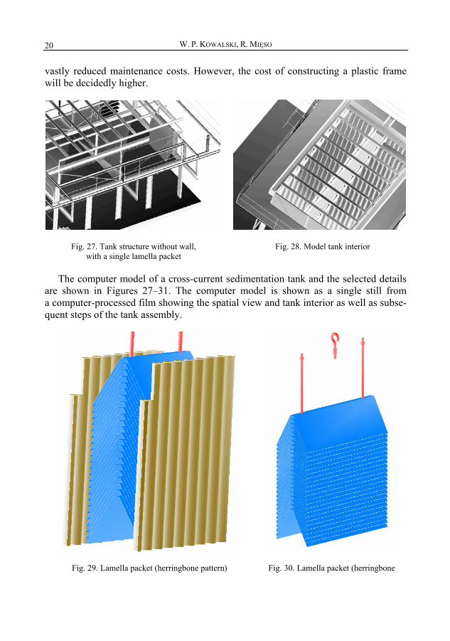
The computer model of a cross-current sedimentation tank and the selected details are shown in Figures 27–31. The computer model is shown as a single still from a computer-processed film showing the spatial view and tank interior as well as subse-quent steps of the tank assembly.
Fig. 29. Lamella packet (herringbone pattern) Fig. 30. Lamella packet (herringbone

Cross-current lamella sedimentation tanks
21
and the chamber wall pattern) and the lifting sling
Main design guidelines: 1. The key element securing the housing in place is the frame made of the standard
C-profiles. The inside diameter of the frame should be 5050 mm in the direction of the main symmetry axis and 3200 mm in the direction of the short axis.
2. Above the frame arranged horizontally, on the edges parallel to the main symmetry axis there are symmetric shelves running inwards to the distance 100 mm (towards the frame axis) to support the lamella packets. Besides, a similar shelf though twice as wide (about 200 mm) should be placed along the longer axis of the frame.
3. Underneath the frame two hollow chambers intended for sediment collection are provided. They are shaped like pyramids, their vertices directed downwards, the side wall inclination 45°.
4. On the vertices of these two pyramids (at the lowest points in the settling cham-ber) there are valves connected with pipes used for removing the sediment. Sediment discharge and its further transport to the basin supplying the feed material to the Dorr clarifier should be induced by a pump with the capacity of 20 m3/h, operated jointly for the two twin tanks.
5. Around the whole tank on the level of the frame there is a platform about 1 m wide for the personnel.
6. A vertical, split clarification chamber shaped like a rectangular prism minus a bottom and roof is on the frame. Its height approaches 1600 mm.
7. The clarification chamber is divided by a vertical baffle coinciding with the main axis of the frame symmetry and supported on a shelf. The baffle should be about 400 mm lower than the longer chamber walls.
8. Clarified suspension flows out along the outside edges parallel to the longer axis of the chamber, that is why shorter wall ought to be higher than the longer ones.
9. The feed supply basin is over the baffle. It should be 400 mm wide and 500 mm high, out of which 100 mm should extend above the liquid level and 400 mm is kept immersed. The bottom of the chamber (in its axis of symmetry) is tangent to the upper edge of the baffle. The connection between the baffle and the basin bottom need not be sealed.
10. The flow of suspension from the Dorr clarifier overflow to the supply basin is induced by the forces of gravity. It is suggested that the suspension flowing in the pipeline over the chamber be distributed in three pipes symmetrical in the plane of the baffle.
11. In the basin bottom, there is a plugged drain, easy to open (similar to the one in a bath tub). It is used to empty the feed basin whilst the whole tank is being emp-tied.
12. Suspension flows from the feed supply basin into two symmetrical sections of the chamber. It flows in the horizontal direction, parallel to the shorter axis of the

W. P. KOWALSKI, R. MIĘSO 22
chamber. The flow path equals 1600 mm (half-width of the chamber). From the chamber filled with lamella packets the suspension flows to the overflow basin.
13. Overflow basins are fixed along the longer walls of the split chamber. On one of the shorter walls there is the trough connecting the overflow basins so that the whole clarified suspension leaves the system.
14. Each of the twin chambers is divided into 10 sections by vertical panels made from corrugated plastic plates, with the wave height of 50 mm. Dividing panels are supported on shelves on the frame level and extend over the liquid table (over 100 mm). Single section dimensions are: 1600 mm (split chamber width) × 500 mm (sec-tion width taking into account the width of a corrugated panel).
15. Each section (including the first and the last one) is surrounded by two parallel corrugated baffles. One baffle is used between each two neighbouring sections (apart from the first and the last one).
16. At the bottom of each section an extra bottom surface is provided: a protective barrier directing the suspension towards the section interior. The barrier is made of PVC board shaped like a sloped roof inclined at 60o with a horizontal ridge 40 mm in width. The barrier length equals the width of the split chamber (identical to the section length equal to 1600 mm). The barrier is supported on shelves lying on the frame.
17. Each section has two saw-tooth edges, their height variable and controllable over 50 mm to ensure the equal chamber loading.
18. On the end of feed basin each section is provided with a guiding barrier, directing the suspension downwards. The guiding barrier is located at the distance of 100 mm from the feed supply basin and extends over the liquid level (about 100 mm), the remaining part (i.e. 500 mm) should be immersed.
19. On the overflow basin end each section has a guiding barrier different from the previous one in that that it should be immersed to the depth of about 200 mm.
20. In each section, there are lamella packets. Packets are arranged in a herring-bone pattern, the elementary unit being a symmetrically shaped profile resembling a roof inclined on both sides and with a flat ridge. The inclination angle of the profile is 60o. The terminal edges are bent at the right angle so that each profile be supported on the previous one. In the bend sections, some openings are cut, accounting for 80–90% of the bend surface. The single packet contains 25 shaped profiles. Shaped pro-files are interconnected by two vertical tubes 1500 mm in length and with the outside diameter 10 mm. These tubes pass through the openings made in the ridges of the shaped profiles. Between the subsequent profiles there are spacing elements (bush-ings) with washers. The height of the spacing elements is 40 mm. In the lowermost tube section, there is a back nut with a washer. In the topmost tube section, a hook is provided to hang the packet. Hooks are hung on a rod coinciding with the section axis, at the height of 200 mm over the liquid level. A screw joint between the hook and the tube enables position control of the packet inside the section (in a range of about 50 mm). The rod is supported on a framework connected to the split chamber. Inside the section the packet is tangent to the ridges of corrugated baffles.

Cross-current lamella sedimentation tanks
23
4. Conclusions
Theoretical studies and computer simulations of cross-current processes in sedi-mentation tanks with lamella packets reveal that tank capacity during clarification of dilute suspensions can be vastly improved if compared with the conventional tanks (even ten-fold increase of process capacity is reported). As regards the lamella counter-current processes, the improvement in performance is two- or even three-fold, in relation to the space they occupy.
It appears, therefore, that cross-current sedimentation tanks can successfully be ap-plied in industrial installations for clarification of suspensions which, on account of the presence of very fine particles or the flow rates, are hard to process because of space limitations and high costs. In many sectors of industry, suspensions are clarified in installations designed many years ago and the achievable sedimentation efficiencies are regarded as insufficient in the light of the present standards. In such cases, the use of cross-current lamella tanks as secondary clarifiers might be the answer to the prob-lem, ensuring the required quality of clarified suspension at relatively low costs, esti-mated to be 20% of costs involved in construction of traditional tanks.
High capacity of cross-current lamella tanks (or improved sedimentation effi-ciency) are achievable by extending the settling surface thanks to the placing of la-mella packet sections at small intervals. The presence of lamella packets causes no problems during the clarification of dilute suspensions though when thickened suspen-sions are handled, the clarification processes might be disturbed.
References
[1] Bandrowski J., Hehlmann J., Merta H., Zioło J.: Opracowanie metody optymalnego do-boru wysokosprawnych osadników z wypełnieniem na podstawie doświadczalnych badań osadników, Inż. Ap. Chem.,1 (1997), 3–8.
[2] Bandrowski J., Hehlmann J., Merta H., Zioło J.: Podział zawiesin ze względu na możli-wość zagęszczania w osadnikach z wypełnieniem oraz analiza czynników wpływających na proces sedymentacji cienkowarstwowej, Inż. Ap. Chem., 3 (1997), 3–7.
[3] Bandrowski J., Hehlmann J., Merta H., Zioło J.: Studies of sedimentation settlers with packing, Chem. Engng. and Proc., 36, (1997), 219–229.
[4] Bandrowski J., Merta H., Zioło J.: Analiza modeli osadników z wypełnieniem, Inż. Ap. Chem., 6, 1995.
[5] Bandrowski J., Merta H., Zioło J.: Sedymentacja zawiesin. Zasady i projektowanie, Wyd. Politechniki Śląskiej, Gliwice, 2001.
[6] Bandrowski J., Merta H., Zioło J.: Analiza modeli osadników z wypełnieniem (in Polish), Inż. Ap. Chem., 6, 1995.
[7] Bandrowski J., Merta H., Zioło J.: Modele osadników z wypełnieniem, Mat. XVI Ogólnopolskiej Konferencji Naukowej Inżynierii Chemicznej i Procesowej, t. 1. Prze-pływy, mieszanie. Procesy dynamiczne z fazą stałą, s. 180–185, Wyd. Politechniki Gdańskiej, 12–15 września 1995.

W. P. KOWALSKI, R. MIĘSO 24
[8] Buer T., Margraf M.: Enhancement of activated sludge plants by lamellas in aeration tanks and secondary clarifiers, Paper presented at the Aeration Conference on Applied Techniques to Optimize Nutrient Removal and Aeration Efficiency, Helsinki, 2000.
[9] Boycott A.E.: Sedimentation of Blood Corpuscles, Nature, 104, 532. [10] Camp T.R.: Sedimentation and the Design of Settling Tanks, Trans. Amer. Soc. Civ.
Engrs, 111, 1946, 895–958. [11] Gęga J.: Wysokosprawne osadniki z wkładami rurowymi do oczyszczania ścieków hutni-
czych, Zesz. Nauk. AGH, 561, 9, 1976, 89–99. [12] Haba J., Nosowicz J., Pasiński A.: Klären und Eindicken von Suspensionen in Lamellene-
neidickern, Aufbereitungs-Technik, 4, 1980, 198–201. [13] Haba J., Nosowicz J., Pasiński A.: Sedymentacja zawiesin w osadnikach płytowych, Rudy
Metali, 23, 9, 1978, 440–444. [14] Haba J., Nosowicz J., Pasiński A.: Wyznaczanie stopnia sedymentacji w osadniku z
wypełnieniem płytowym, Rap. Inst. Inż. Chem. Urz. Ciepl. Polit. Wrocł., seria preprints, 91, Wrocław, 1980.
[15] Haba J., Pasiński A.: Badanie osadnika płytowego w zastosowaniu do technologii otrzymywania wodorotlenku glinu, Rap. Inst. Inż. Chem. Urz. Ciepl. Polit. Wrocł., 4, Wrocław, 1979.
[16] Hazen A.: On Sedimentation, Trans. ASCE, 53, 1904, 45–88. [17] Kowalski W.: Mathematical model of sedimentation process in the bended suspension
stream (in Polish), Arch Ochr. Środ., 1–2, 109–120, 1991. [18] Kowalski W.: Parameters of the particles composition of the emitted dust from iron
metallurgy processes (in Polish), Arch. Ochr. Środ., 1–2, 67–79, 1991. [19] Kowalski W.: Sedimentation balance – interpretation method of information about parti-
cle composition (in Polish), Arch. Ochr. Środ., 1–2, 1991, 159–167. [20] Kowalski W.: Generalization of Hazen’s Sedimentation Theory, Archives of Hydroengi-
neering, Vol. XXXIX, 2, 1992, 85–103. [21] Kowalski W.P.: Analiza teoretyczna i badania procesu sedymentacji wielostrumieniowej
(in Polish), Problemy Inżynierii Mechanicznej i Robotyki, 3, Kraków, 2000, 179. [22] Kowalski W.P.: Podstawy teoretyczne projektowania osadników z wkładami
wielostrumieniowymi (in Polish), Zeszyty Naukowe AGH, seria Mechanika, 27, Kraków, 1992, 132.
[23] Kowalski W. P.: Modelowanie matematyczne procesu sedymentacji ziaren zawiesin polidyspersyjnych, Mat. XLIII Sympozjonu pt. „Modelowanie w mechanice” (in Polish), Gliwice, 2004.
[24] Kujawska E.: Badania procesu sedymentacji w osadniku z wypełnieniem płytowym i profilowym, PhD Thesis, Politechnika Śląska, 2003.
[25] Niedźwiedzki Z.: Badania teoretyczne i eksperymentalne wypełnień osadników wielostru-mieniowych, Zesz. Nauk. Politechniki Łódzkiej, 863, Łódź, 2000, 162.
[26] Merta H.: Projektowanie osadników z wypełnieniem. Część 1. Parametry projektowe i technologiczne osadników płytowych i rurowych oraz ich klasyfikacja (in Polish), Inż. Ap. Chem., 2, 1996, 3–10.
[27] Nipl R.: O zastosowaniu uogólnionego rozkładu gamma do aproksymacji krzywych składu ziarnowego, Mat. XIII Krakowskiej Konferencji Nauk.-Techn. Przeróbki Kopalin (in Polish), Kraków, 1979, 323–330.

Cross-current lamella sedimentation tanks
25
[28] Olszewski W.: Osadniki wielostrumieniowe, [in:] Nowa Technika w Inżynierii Sanitarnej (in Polish), Wodociągi i Kanalizacja, t. 5, 1975.
[29] Oden S.: Eine neue Methode zur Bestimmung der Kornerverteilung in Suspensionen, Kol-loid -Z , 18, 2, 1916, 33–47.
[30] Orzechowski Z.: Przepływy dwufazowe, jednowymiarowe, ustalone, adiabatyczne, PWN, Warszawa, 1990.
[31] Papoulis A.: Prawdopodobieństwo, zmienne losowe i procesy stochastyczne, wyd. l, WNT, Warszawa, 1972.
[32] Mięso R.: Badania prostopadłoprądowego procesu sedymentacji, PhD Thesis, AGH, Kraków, 2000.
[33] Stacy E.W.: A Generalization of the Gamma Distribution, Annals of the Mathem. Statis-tics, Vol. 33, 3, 1962.
[34] Stokes G.G.: On the Effect of the Internal Friction of Fluids on the Motion of Pendulums, Camb. Trans., Vol. 9.
[35] Materiały informacyjne firmy Sala Inc. [36] Zioło J.: Influence of the system geometry on the sedimentation effectiveness of lamella
settlers, Chem. Engng. Sci., Vol. 51, 1, 1996, 149–153.
Prostopadłoprądowe osadniki wielostrumieniowe
Przedstawiono genezę urządzeń sedymentacyjnych opartych na wykorzystaniu efektu Boy-cotta. Opisano trzy podstawowe układy, w jakich prowadzi się sedymentację wielostrumie-niową. Są to: układ przeciwprądowy, prostopadłoprądowy i współprądowy. Poprawę efektyw-ności sedymentacji w osadnikach z wkładami wielostrumieniowymi osiąga się, zwiększając powierzchnię sedymentacyjną.
Miarą zwiększenia powierzchni sedymentacyjnej jest wskaźnik wyrażony przez stosunek pola powierzchni sedymentacyjnej zawartej w pakiecie do podstawy pakietu, nazywany po-wierzchnią właściwą. Przedstawiono typową konstrukcję pakietu wielostrumieniowego dla se-dymentacji przeciwprądowej. Ograniczenia konstrukcyjne (zwiększanie długości przewodu z jednoczesnym zmniejszaniem jego przekroju poprzecznego) i wykonawcze powodują, że nie da się osiągnąć wskaźnika powierzchni właściwej o wartości wyższej od 5–6, a ponadto prze-pływ zawiesiny w przewodach o długości względnej l/d > 10 osiąga zakres dużych liczb Rey-noldsa i przestaje być laminarny. Można jednak zastosować inną koncepcję rozwiązania kon-strukcyjnego pakietów opartą na wielostrumieniowej sedymentacji prostopadłoprądowej. W tym przypadku ograniczenia konstrukcyjne i wykonawcze nie stanowią przeszkody, pakiet jest, bowiem stosem płyt o teoretycznie nieograniczonej wysokości.
W artykule opisano oryginalne stanowisko do badań sedymentacji prostopadłopradowej. Przedstawiono także matematyczny model procesu sedymentacji prostopadłoprądowej, wyniki badań oraz wyniki symulacji komputerowych. Wyniki badań i symulacji komputerowych pro-wadzą do wniosku, że w osadnikach tego typu można nawet ponad 10-krotnie zwiększyć wy-dajność lub adekwatnie podnieść efektywność sedymentacji. Na podstawie badań i obliczeń przedstawiono komputerowy projekt osadnika prostopadłoprądowego o wydajności 100 m3/h. Urządzenie tego typu zajmuje około 10% miejsca niezbędnego dla tradycyjnych urządzeń se-dymentacyjnych i pozwala osiągnąć dużą efektywność porównywalną z efektywnością trady-cyjnych urządzeń. Dlatego może być stosowane do wysokosprawnego i wysokowydajnego kla-

W. P. KOWALSKI, R. MIĘSO 26
rowania zawiesin przemysłowych lub zawiesin pochodzących z obiegu uzdatniania wód i oczyszczania ścieków, zwłaszcza w przypadkach, gdy jest brak miejsca na urządzenia trady-cyjne lub gdy dąży się do obniżenia kosztów budowy i eksploatacji osadnika.

ARCHIVES OF CIVIL AND MECHANICAL ENGINEERING
Vol. IV 2004 No. 4
The analysis of brushing tool characteristics
S. SPADŁO Kielce University of Technology, al. Tysiąclecia P. P. 7, 25-314 Kielce
In this paper, an analytical procedure is developed in order to evaluate the filament loading of a circular brush. Filament deformation is computed based on the mechanic analysis in conjunction with kinematic con-straints for a rigid flat surface with friction taken into account. Numerical results which reveal the relationship between rotation angle and force distribution are reported.
Keywords: flexible electrode, filament, interaction forces
1. Introduction
So far the machining process using filamentary metal brushes in the shape of disks has been used in surface machining to remove corroded layers, to prepare metal surfaces to be galvanized, and to produce surfaces of high adhesion to be coated with paint, glue, etc. Recently the process has been developed to include operations such as removing sharp edges and burrs [1,10], flashes and bosses from machine parts made of alloys of non-ferrous metals, as well as cleaning welds. Using brushes with densely packed filaments made of hard steel broadens the range of uses to include the micro-milling of ordinary constructional steels of low hardness, which are machined with the tips of the filaments. To summarize, the typical uses of metal brush tools are limited to machining materials whose hardness is lower than that of the material the filaments of the brush are made of.
Using the filaments made of abrasive-grain-filled polymers allows the brushes to be used to machine the surfaces of materials of high hardness.
On analysis of the advantages of using brush tools the author suggests a new ma-chining operation that combines mechanical, electrochemical, and electro-erosive processes acting on the machined item [3–6].
Due to the synergistic effect this type of hybrid machining makes the metal re-moval process more cost-effective.
Soft-machining parameters allow not only the removal of the excess material from large items of low stiffness but also the highly efficient volumetric machining of met-als, alloys, and conductor-based composites.
The numerous uses of brush electrodes result from such their characteristics as: • flexibility of individual filaments, • type, shape, and packing density of the filaments, • possibility of operating at various settings of electrode deflection,

S. SPADŁO 28
• large contact zone of the tool and the machined item, • possibility of using the electrode until it is worn out, • large working area of the hot electrode allowing the machining of both flat and
complex-shape items. Because of their construction brush electrodes are characterized by: • uniform distribution of the filaments, which helps to form a discrete structure
suitable for maintaining stable conditions in the machining zone, • radial, axial, and tangential flexibility, which makes the filaments fit easily com-
plex geometry surfaces, thus permitting a uniform removal of surface layers without changing significantly the geometry of the machined part,
• easy disposal of the erosion by products from the discharge zone, • suitability for automated operations. The use of brushing tools in an automation environment will necessitate a clear un-
derstanding of an important characteristics of brush performance such as forces. An understanding of such characteristics is important, as surface preparation processes re-quire a detailed knowledge of interrelationships between productivity of machining and brush operating conditions [3, 7]. For example, it is recognized that electrical dis-charges generated during electroerosion-mechanical processes are closely related to the mechanical characteristics of the filament [5].
2. Statics and kinematics of a single filament
Since the elements of a disk brush tend to deform easily, the use of the brush in erosion mechanical machining changes the character of mechanical interactions with the machined surface in contrast to deformation-resistant electrodes. An increase in the value of the pressure force at the filament tip as a function of displacement along the surface inevitably leads to a break in the anodic film and initiates discharges whose frequency can be determined, among others, by the vibrations of individual filaments of the electrode.
The mechanics of the movement and the interactions between the filament wire and the machined surface are very complex. The wire becomes deformed in a way that is difficult to analyse. This is caused by confounded boundary conditions which allow only an approximate solution to the equation of its motion.
Only a tentative analysis of the interactions between the brush elements and the surface has been presented.
Let us consider a tentative analysis of a filament load. The basic assumptions are: • inertial forces are neglected, • the filament tip moves along a rigid surface.
Additionally, due to low packing density, interactions between individual wires are ignored. It is assumed that the filaments are placed radially from the hub centre and are restrained at the hub outside radius and obey Hooke’s law [8].

The analysis of brushing tool characteristics
29
The filaments are straight before they come into contact with the machined surface. They are deflected perpendicularly to the axis of rotation, with the radial run-out of the disks being ignored.
Filament deflection is examined in a mobile reference system K ξ η (Figure 1), where η = η (ξ) is its elastic deflection assuming that there is no influence of non-di-latational strain.
r
O K Px
Pξ
O x
y
b
l
η
ω0
ξ
η
ξ ξ
η
Pη x
y
K h f
α0 α
PyS
a
Fig. 1. Geometry of a particular filament deformation
The differential equation of the bending line is:
)],()([)()1( 2/32 ξηηξ
ηη
ξη −+−=′+′′
bFbFEI (1)
where: EI – filament flexural rigidity,
ξηξη dd /)( =′ ,
22 /)( ξηξη dd=′′ ,
b≤≤ ξ0 .
The geometry of the problem examined produces the following relationships:
αsin/fh = ;

S. SPADŁO 30
ααα
coscossin
hdhrrab +=+−+
= ,
.sin
rrad −+
=α
We assume that:
,xy FF µ=
xFcF 1=ξ ,
xFcF 2=η ,
αµα cossin1 −=c ,
,sincos2 αµα +=c
where: t0ωα = ,
µ – coefficient of friction between the filament tip and the machined surface, ω0 – angular velocity of the brush. The function η(ξ ) should also satisfy the following condition:
0)]([10
2 =′+− ∫ ξξη dlb
. (2)
It is very difficult to obtain numerical solutions for Equation (1) with constraint (2). Analytical solutions can be obtained if the values of η(ξ ) are small enough to enable the linearization of the left-hand side of Equation (1).
The details of the solution of Equation (1) with initial conditions:
0)0( =η and 0)0(' =η
and with the assumption that the wire tip (for ξ = b) has point contact with the surface (then η"(b) = 0)) have been presented below.
We will examine a case of a single filament load under tentative conditions pre-sented above. The deflection of the part is described in a mobile reference system K ξ η (Figure 1). In such a case, η = η(ξ ) is its elastic deflection with the assumption that there is no influence of non-dilatational strain.

The analysis of brushing tool characteristics
31
An approximate analytical solution can be obtained if we assume that the values of )(' ξη are small enough to enable the linearization of the left-hand side of Equation
(1), which is the case where:
.1<<−l
al
Then we assume that:
.1)(' <<ξη
Consequently, in place of Equations (1), (2) we can have
[ ,)()()()(231 12
2xFfCbCEI ηξξηξη −+−=′′⎥⎦
⎤⎢⎣⎡ ′− ] (1a)
[ ] ,0)(21 2
0
=′−− ∫ ξξη dblb
(2a)
where:
)(bf η= .
As a result of a subsequent approximation the above equations are replaced by:
[ xFfcbcEI )()( 12 ]ηξη −+−=′′ (3a)
[ ] bldb
−=′∫ ξξη 2
0
)(21
. (3b)
Furthermore, we will consider solutions for Equations (3) valid only if l–a is small. The first equation is as follows:
[ ]EIFccfccdc x
ηξαη 12122 )ctan( −−++=′′
and we assign:
EIFc x12 =ω ,

S. SPADŁO 32
,1
2
cEIFx ω
=
thus
[ ] ,)ctan( 2
1
2
1
2
121222 ξωωηξαωη
cc
cccfccdc −−−++=+′′
because
,sin/1ctan 12 αα =+ cc
so
,2
1
22 ξωηωηccD −=+′′ (4)
where:
const=+=1
2
2 )(c
hdcD ω (does not depend on ξ).
The solution to Equation (4) with initial conditions:
0)0( =η and 0)0(' =η
and with the wire tip (ξ = b) having point contact with the surface (then η"(b) = 0) is:
[ ,)sin(tan)cos1(1)()()(
1
2 ξωωξωωξωα
αξη +−−= bcc ] (5)
where:
.)(12
IEFc xα
ω =
The problem is intractable because: • ω is unknown (dependent on the unknown Fx) • and b is unknown (dependent on h or f ).

The analysis of brushing tool characteristics
33
In (4), we should require for ξ = b to be η (b) = f = h⋅sinα, then we obtain:
[ ] ).()sin(tan)cos1(1)()(sin
1
2 bbcch ηωξωξωωξ
ωααα =+−−=
Thus, after employing geometric relationships, we obtain the following equation:
bcbbbdchωαω
ωωtancos
)(tan
2
2
−−
= . (6)
Condition (4) will be satisfied after employing (5), so the equation is rewritten as:
⎥⎦
⎤⎢⎣
⎡−
−=′ 1
cos)(cos)(
1
2
bb
cc
ωξωξη ,
then
[ ] .2tan3cos
12
)(21
2
2
1
2
0
2 bb
bbc
cdb
⋅⎟⎟⎠
⎞⎜⎜⎝
⎛+−⎟⎟
⎠
⎞⎜⎜⎝
⎛=′∫ ω
ωω
ξξη
Employing
ααα
coscossin
hdhrrab +=+−+
=
we obtain:
.2tan3cos
1cossin
1 2 bb
bb
hrra⋅⎟⎟⎠
⎞⎜⎜⎝
⎛+−=−+
+−
ωω
ωα
α (7)
Substituting (6) for (7) we obtain a transcendental equation with the unknowns ω b. Only the lowest roots of the equation calculated as a function of α are physically fea-sible. These roots enable the value of ω to be calculated.
It applies to all the components of the interaction force, that is:
1
2
cEIFxω
= , ,xy FF µ=

S. SPADŁO 34
xFcF 1=ξ , ,2 xFcF =η
as well as to the bending line for η(ξ ).
Fig. 2. Changes in the parameter ωb as a function of the rotation angle and filament flexural rigidity
Figure 2 shows the changes in the parameter ωb as a function of α = ω0 t and filament flexural rigidity EI at the following parameters: l = 0.05 m, a = 0.04 m, r = 0.02 m, µ = 0.5.
Fig. 3. The values of force component Fx, interaction with the surface as a function of rotation angle α and filament flexural rigidity EI

The analysis of brushing tool characteristics
35
Fig. 4. The values of force component Fy, interaction with the surface as a function of rotation angle α and filament flexural rigidity EI
Graphs of the changes in the values of force components Fx, Fy as a function of the rotation angle and filament flexural rigidity EI have been presented in Figures 3–4.
Graphs of the changes in the values of force components Fξ, Fη as a function of the rotation angle and filament flexural rigidity EI have been presented in Figures 5–6.
Fig. 5. The values of force component Fξ, interaction with the surface as a function of rotation angle α ------------------ -------------- and filament flexural rigidity EI

S. SPADŁO 36
Fig. 6. The values of force component Fη, interaction with the surface as a function of rotation angle α and filament flexural rigidity EI
The changes in the relationship Fη as a function of the angle α = α(t) have to be pointed out. At α ≈ 116o the sign of the force is reversed. Consequently, the force causes the filament to straighten when it loses contact with the machined surface.
3. Dynamics of a single filament of a circular filamentary brush
The equation of the motion of a filament with its mass taken into account can be shown by coordinates K ξ η as an equation [2] describing relative motion. We assume that |η(ξ, t)| << 1 and omit Coriolis inertial forces which are negligibly small in this case in order to obtain:
αξρξδ∂η∂ρ
ξ∂η∂
ξ∂η∂
ηξ &&)()(12
2
2
2
14
4
++−−=++ rAbFt
AFEI . (8)
It can be shown that when inertial forces are neglected the equation can be rewrit-ten as (3a). Forces Fξ and Fη are marked Fξ1 and Fη1, respectively, because these are not the same forces as in the previous expressions.
Solutions have to be looked for with boundary conditions being:

The analysis of brushing tool characteristics
37
for 0)0( =ξ we have 0),0( =tη and 00=∂∂
=ξξη
,
for )(tb=ξ we have 0)(2
2
=∂∂
= tbξξη and 1)(3
3
][1 ηξξ ξη
ξη FFEI tb −=
∂∂
+∂∂
= ,
and initial conditions:
0)0,( =ξη , 00=∂∂
=ttη
.
(9)
In addition, the geometric conditions mentioned earlier have to be met as well as condition (2). This boundary-initial problem cannot be solved by conventional meth-ods. It is very hard to obtain even approximate numerical solutions for the equation.
If we assume that the filaments maintain contact with the machined surface, the following condition is satisfied:
[ ] bldb
−=′∫ ξξη 2
0
)(21 . (10)
It is very hard to obtain even approximate solutions for the equation. This boundary-initial problem cannot be solved by conventional methods. Based
on the solutions presented above, the Galerkin approximation was used. At α = ω 0 t the last component of Equation (8) disappears.
Let us assume that the first approximation is
)()(),( tSYt ⋅≈ ξξη , (11)
where: the value S(t) describes the shift of the filament tip towards the axis η when is mul-
tiplied by Y(b), the function of Y(ξ ) has been chosen arbitrarily; it satisfies the conditions Y(0) = 0
and Y'(0)=0 and will be integrated using the variable limits of 0 – b(t). As a result we obtain an ordinary differential equation containing variable coeffi-
cients because
),()( tbbb == α
( ) ( ) ( ) ( ) ( ),1 bYFtSbktSbm rr η−=⋅+⋅ && (12)
S. SPADŁO 38
where:
ξξρ dYAmb
r )(2
0∫= ,
∫ ∫+=b b
r dYYFdYYEIk0 0
1 )()()()( ξξξξξξ ξIIIV ,
whose solution should satisfy condition (10). Consequently, we obtain a system of two equations with two unknowns S(t) and b(t).
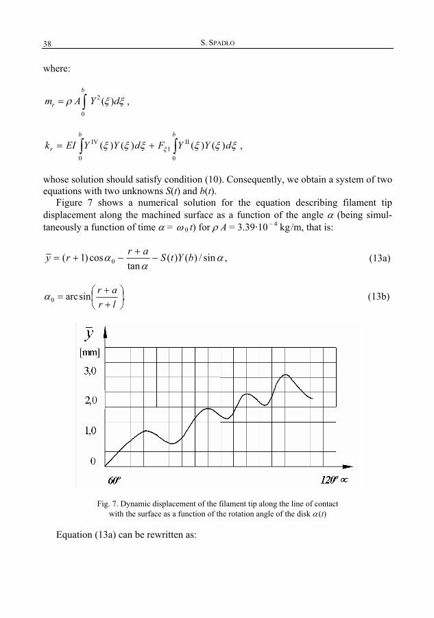
Figure 7 shows a numerical solution for the equation describing filament tip displacement along the machined surface as a function of the angle α (being simul-taneously a function of time α = ω 0 t) for ρ A = 3.39⋅10 – 4 kg/m, that is:
,sin/)()(tan
cos)1( 0 αα
α bYtSarry −+
−+= (13a)
.sin0 ⎟⎠⎞
⎜⎝⎛
++
=lrararcα (13b)
Fig. 7. Dynamic displacement of the filament tip along the line of contact with the surface as a function of the rotation angle of the disk α (t)
Equation (13a) can be rewritten as:

The analysis of brushing tool characteristics
39
,sin/)()(tan
cos 0 αα
α bYtS∆rRy −−
−=
where: R – the disk outside radius, ∆ – the filament radial deflection value applied. Figure 7 shows that the movement of the filament along the machined surface is
not monotonic. It demonstrates that the influence of the filament dynamics on its load can be quite considerable. The paper offers only a brief outline of the problem which requires further research.
4. Conclusions
• Lower packing densities of filament wires diminish the effect of mutual filament support, thus making the brush more deformation-prone. It makes it possible to adjust the deflection (∆) parameter within a wider range of settings, with the disk retaining its original size.
• The pressure force the filament tip exerts on the surface along the displacement path increases in a non-linear manner, with its value suddenly dropping towards the end of the displacement path.
• Upon analysis of the differential equation of a single filament displacement path it can be stated that: − changes of the force of the filament interactions with the surface are directly
proportional to the changes of the filament stiffness, thus a solution for (EI )1 is also applicable to (EI )2, − the shapes of the bending line are identical if for a given position of a workpart
(specified by the angle α) the values of interaction forces (F(α)i) are proportional to the corresponding stiffness values of the elements (EI )i. References
[1] Duwell E.J., Bloecher U.: Deburring and Surface Conditioning with Brushes Made with Abrasive Loaded Nylon Fiber, Society of Manufacturing Engineers, Technical Paper MR83-684, Dearborn, MI. 1983.
[2] Gutowski R., Swietlicki W. A.: Dynamika i drgania układów mechanicznych, PWN, Warszawa, 1986.
[3] Nowicki B., Spadło S.: Smoothing the surface by brush electrodischarge mechanical ma-chining – BEDMM, Central European Exchange Program for University Studies Project PL-1- CEEPUS, Science Report, Kielce, 1998, pp. 129–137.
[4] Spadło S.: Complex Shape Surface Finishing Process, Patent PL 172559, 1997.

S. SPADŁO 40
[5] Nowicki B., Pierzynowski R., Spadło S.: New Possibilities of Machining and Electrodi-scharge Alloying of Free-Form Surfaces, Journal of Materials Processing Technology, 2001, Vol. 109, No. 3, pp. 371–376.
[6] Nowicki B., Pierzynowski R., Spadło S.: The Superficial Layer of Parts Machined by Brush Electrodischarge Mechanical Machining (BEDMM), Proceedings of II International Conference on Advances in Production Engineering. Part II, Warsaw, June, 2001, pp. 229–236.
[7] Spadło S.: Experimental Investigations of the Brush Electrodischarge Mechanical Ma-chining Process – BEDMM, Advances in Manufacturing Science and Technology, Quar-terly of the Polish Academy of Sciences, 2001, Vol. 25, No. 3, pp. 117–135.
[8] Osiecki J., Spadło S.: A model of mechanical interactions of a brush electrode with a flat surface, Proc. of 9th Int. Sci. Conf. on Production Engineering, Computer Integrated Manufacturing and High Speed Machining, Croatian Association of Production Engi-neering, Lumbarda, 2003, pp. IV066–IV072.
[9] Timoshenko S.P., Gere J.M.: Theory of Elastic Stability, second edition, McGraw-Hill, Inc., London, 1961, pp. 76–81.
[10] Wick C., Veilleux R.F.: Mechanical and Abrasive Deburring and Finishing, SME Tool and Manufacturing Engineers Handbook, Chapter 16, Vol. 3, 1985.
Analiza charakterystyk narzędzi szczotkowych
Przedstawiono analityczne rozwiązanie zagadnienia sił, z jakimi oddziaływują pojedyncze włókna szczotki obrotowej z powierzchnią. Przeprowadzono analizę deformacji pojedynczych drucików szczotki, uwzględniając występujące więzy kinematyczne dla przypadku powierzchni płaskiej niepodatnej z występowaniem tarcia. Przedstawiono wyniki symulacji komputerowych w postaci zależności sił oddziaływań drucików z powierzchnią w funkcji kąta obrotu szczotki.

ARCHIVES OF CIVIL AND MECHANICAL ENGINEERING
Vol. IV 2004 No. 4
Full-scale laboratory tests and FEM analysis of corrugated steel culverts under standardized railway load
B. KUNECKI, E. KUBICA Wrocław University of Technology, Wybrzeże Wyspiańskiego 25, 50-370 Wrocław
This paper describes a full-scale static test conducted on a corrugated steel culvert with 2.99 m span and 2.40 m in height. The test was carried out in the Bridge and Road Research Institute, Wrocław Branch, Poland, in 1998 for a Norwegian producer of culverts. The standardized railway load configura-tion UIC 71 for Europe was applied at various soil cover (from 0.3 m to 1.0 m). Several full-scale tests have been performed in the field to validate the long-term performance and great load bearing capacity of these structures, but few structures have been tested in controlled conditions in a test facility like the test in Poland. In order to verify the test results, a finite element model for the structures tested was con-structed. The empirical results obtained were compared with results obtained by means of the Finite Ele-ments Method (FEM). To perform the FEM analysis Cosmos/M system software was used. Only results obtained at 0.8 m soil cover were presented and compared.
Keywords: steel culverts, FEM, instrumentation, full-scale test
1. Introduction
Corrugated steel culverts are increasingly being used in road and railway projects as an alternative solution to concrete bridges and culverts. Their construction period is short, and the structures have both technical and economical advantages. Several full-scale tests have been carried out in the field to validate the long-term performance and load bearing capacity of these structures [4, 9]. In contrast to that, only few tests of life-size structures have been performed under fully controlled laboratory conditions.
The experimental data obtained under such conditions are needed in order to verify software tools used for numerical analysis as well as to help us to optimize and design more economic structures. This is of the first importance having high-quality test results when designing flexible, long-span buried structures with minimum cover for live railway and road loads.
2. Description of the structure tested
The structure tested was located in the test stand which is shown in Figure 1. The test stand has the form of an 80 m long and 12 m wide reinforced concrete foundation with a system of anchors and a steel frame serving as a support structure for the sys-tem of two hydraulic servos with a modern control and feeding system ensuring full control over the static and dynamic loads in real time. The culvert tested had

B. KUNECKI, E. KUBICA 42
a span of 2.99 m, a height of 2.40 m and a length of 14.4 m. Soil cover of 0.80 m was used while standardising railway loads. The steel material was of FE 360 B FN quality to meet European Standard EN 10025. The minimum yield stress was 245 MPa. The corrugation was 150×50 mm and the steel thickness was 3.75 mm [2]. The steel plates were joined by the bolts, 20 mm in diameter, with minimum tensile strength of 830 MPa. The bolts and the joint are shown in Figure 2, and the properties of steel plate are listed in Table 1.
Fig. 1. View of the culvert tested Table 1. Properties of steel plate
Plate thickness [mm]
Area A [mm2/mm]
Moment of inertia I
[mm4/mm]
Section modulus W
[mm3/mm]
Radius of gyration i
[mm]
3.75 4.72 1479.8 55.1 17.7
Fig. 2. Cross-section of the steel plate and the bolts

Full-scale laboratory tests and FEM analysis of corrugated steel culverts
43
The test bin was 12 m long, 5 m wide and 4 m high. It was constructed from rail-way sleepers and steel beams. The test bin was backfilled with a well-graded material with maximum grain size of 32 mm. The backfill was placed in layers with maximum thickness of 20 cm before compaction. The required degree of compaction was 97% Standard Proctor, expected for the 500 mm closest to the structure, where 94% Stan-dard Proctor was sufficient. The cross-section of the test stand is shown in Figure 3.
Fig. 3. Cross-section of the culvert tested
3. Loads
The loads from two hydraulic actuators were distributed through two layers of wooden sleepers and 20 mm thick steel plate with area of 2.60 m × 3.15 m. The cross-section and view of load distribution system are shown in Figure 4.
The standardised configuration of railway loads UIC 71 for Europe was applied. Due to the distribution effect of rails, sleepers and ballast bed, the axle loads from the locomotive (4×250 kN) produce a uniform area load which equals approx. 52.0 kN/m2 at a base of the ballast bed at a depth of 0.5 m. At a depth of 0.8 m the area load is 51.0 kN/m2. The dynamic load factor (European Standard) is 1.37 according to the formula with 0.8 m cover. The resulting pressure which was used in railway standard static test equalled 51.0 × 1.37 = 69.87 kN/m2. A real force used in each actuator is listed in Table 2. Three standard static loads were applied at regular time intervals (about 20 minutes).

B. KUNECKI, E. KUBICA 44
Fig. 4. Cross-section and view of load distribution system
Table 2. Loads Number of
loads Soil
cover h Dynamic factor φ
Area of rigid plate
Total force for two actuators F
Total pressure p
[-] [m] [-] [m2] [kN] [kN/m2] 3 0.8 1.37 8.19 572 69.84
4. Instrumentation and measurement
The instrumentation comprised the following: strain gauges on the inside of metal culvert allowing axial and bending strains to be measured; earth pressure cells allow-ing a total stress in the soil to be measured; displacement gauges inside culverts. A de-tailed description of instrumentation is presented below.
4.1. Strain gauges
Strain gauges were placed at 14 locations inside the steel structure. Two gauges were fitted to each location, one at the top of the corrugation and one at the bottom (total 28 strain gauges). The location of all strain gauges is shown in Figure 5a. This configuration allowed axial and bending strains to be measured. Dummy gauges were installed to provide temperature compensation. Electroresistant strain gauges of the Hottinger Baldwin Masstechnik 6/120LY41 type were installed. Strain gauges had 6 mm measuring base, resistance of 120 Ω and factor k equal to 2.02. The measure-ments were preformed with the use of the tension-metric bridge UPM 100 also from the Hottinger Baldwin Masstechnik. The UPM 100 was connected to Macintosh com-puter equipped with “Beam” software.
4.2. Earth pressure cells
Earth pressure around steel structure was measured by earth pressure cells. In order to specify the pressure in the surroundings of culvert, ten earth pressure cells were in-stalled in the soil. Eight of them were installed at steel structures, about 6 cm from
Full-scale laboratory tests and FEM analysis of corrugated steel culverts
45
steel plates. Additionally two earth pressure cells were installed on the top of both sides of the structure at a distance of 1.5 m from symmetry axis. The location of all earth pressure cells is shown in Figure 5b. Each cell is sheltered by 0.03 m layer of dry sand and durable foil. View of earth pressure cells during installation is shown in Fig-ure 6. Magnetoelastic pressure cells from Wrocław University of Technology were used. Measure system PPN-3 with “Dynusing” software was used for data collecting from gauges.
4.3. Displacement gauges
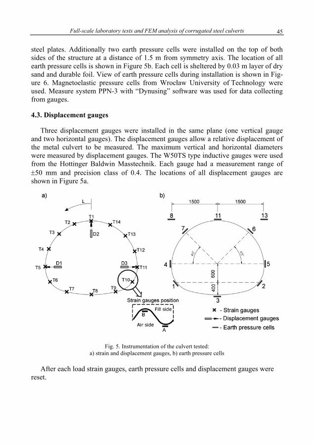
Three displacement gauges were installed in the same plane (one vertical gauge and two horizontal gauges). The displacement gauges allow a relative displacement of the metal culvert to be measured. The maximum vertical and horizontal diameters were measured by displacement gauges. The W50TS type inductive gauges were used from the Hottinger Baldwin Masstechnik. Each gauge had a measurement range of ±50 mm and precision class of 0.4. The locations of all displacement gauges are shown in Figure 5a.
Fig. 5. Instrumentation of the culvert tested: a) strain and displacement gauges, b) earth pressure cells
After each load strain gauges, earth pressure cells and displacement gauges were reset.

B. KUNECKI, E. KUBICA 46
Fig. 6. View of earth pressure cells during installation
5. Test results
All test results from displacement, earth pressure and strain gauges are listed in Ta-bles 3, 4, 5. There are shown the values from three loads and average value. All of them were obtained 20 s after reaching a full load assumed.
The stresses in steel structure were calculated based on strains taking into consid-eration that the elastic modulus of steel is Es = 205 GPa. The stresses at each meas-urement point (two of strain gauges) were allocated to axial stresses and bending stresses according to the known equations:
2BA
aσσσ +
= , (1)
2BA
bσσσ −
= , (2)
where: σa – axial stresses, σb – bending stresses, σA – stresses in the point A (at the crest of corrugation), σB – stresses in the point B (at the valley of corrugation).

Full-scale laboratory tests and FEM analysis of corrugated steel culverts
47
Table 3. Displacement [mm] Gauges D1 (left) D2 (top) D3 (right) Load I 1.16 –2.55 1.12 Load II 0.85 –2.24 1.00 Load III 0.83 –2.19 0.98 Average 0.95 –2.33 1.03
Table 4. Earth pressure [kPa]
Gauges 1 2 3 4 5 6 7 8 11 13 Load I 57.2 56.4 0.1 32.2 27.0 22.2 27.4 32.6 29.1 50.2 Load II 51.2 49.8 0.1 31.9 27.4 21.1 26.4 31.3 25.8 50.7 Load III 49.8 48.7 0.1 32.1 27.0 20.9 26.1 30.9 25.3 50.1 Average 52.7 51.6 0.1 32.1 27.1 21.4 26.6 31.6 26.7 50.3
Table 5. Axial stress (N ) and bending stress (M ) [kPa]
Load I Load II Load III Average Gauges
N M N M N M N M T1 –5.806 0.122 –5.947 0.092 –5.947 0.092 –5.900 0.102 T2 –2.903 0.058 –3.398 0.055 –3.398 0.056 –3.233 0.056 T3 –9.275 –0.119 –9.487 –0.111 –9.416 –0.116 –9.393 –0.115 T4 –10.054 –0.062 –10.054 –0.050 –9.841 –0.051 –9.983 –0.054 T5 –6.868 –0.099 –6.655 –0.092 –6.584 –0.088 –6.702 –0.093 T6 0.425 0.131 0.354 0.114 0.354 0.114 0.378 0.120 T7 –0.354 0.011 –0.496 0.009 –0.354 0.009 –0.401 0.010 T8 –0.425 –0.002 –0.425 –0.003 –0.496 –0.001 –0.448 –0.002 T9 0.354 0.012 –0.354 0.011 –0.354 0.012 –0.118 0.012
T10 –0.071 0.131 –0.283 0.113 –0.142 0.115 –0.165 0.120 T11 –8.142 –0.115 –7.788 –0.106 –7.717 –0.102 –7.882 –0.108 T12 –11.257 –0.080 –10.903 –0.063 –10.832 –0.064 –10.998 –0.069 T13 –11.186 0.124 11.045 –0.129 –10.903 –0.135 –3.682 –0.047 T14 –7.151 0.078 7.292 0.087 –7.080 0.093 –2.313 0.086
6. Modelling of the structure
Analyses of the soil–structure system were carried out using the computer software Cosmos/M system. The computer software allows the simulation of live loads only. The Cosmos/M software allows the simulation of live loads together with deadweight of soil and structures as well.
The finite elements and static model of soil–structure system is shown in Figure 7. Only half of the system was modelled, as the geometry and loading were essentially symmetric. The culvert structured was modelled by 32 Beam2D elements, and the soil by 316 Plane2D elements.

B. KUNECKI, E. KUBICA 48
Fig. 7. Finite element modelling of culvert, soil and test bin
6.1. Element Beam2D
Beam2D is a 2-node uniaxial element for two-dimensional structural. The element has three degrees of freedom (two translations and one rotation) per node for structural analysis. All elements have to be defined in the X–Y plane as shown in Figure 8. Output results are the following: forces, moments, and stresses are available in the element coordinate system.
Fig. 8. Beam2D element

Full-scale laboratory tests and FEM analysis of corrugated steel culverts
49
Real constants used in Beam2D element are: r1 – cross-sectional area (A), r2 – moment of inertia (Jx), EX – modulus of elasticity in the 1st material direction, NUXY – Poisson’s ratio relating the 1st and 2nd material directions, DENS – density.
6.2. Element Plane2D
Plane2D is a 4- to 8-node two-dimensional element for plane stress, plane strain, or axisymmetric structural with symmetric and non-symmetric (asymmetric) loading. All elements have to be defined in the X–Y plane. Only two translational degrees of free-dom per node are considered for structural analysis. The nodal input pattern is shown in Figure 9 for an 8-node element illustrating its local node numbering. The element however can be used with 4- to 8-nodes by assigning zeros (0) at the locations of missing nodes during element connectivity definition. Triangular in shape elements can also be considered. In this case, the third and the fourth nodes (in case of 4-node elements) and the third, the fourth and the seventh nodes (in case of 5- to 8-node ele-ments) will be assigned the same global node number as shown in Figure 9.
Fig. 9. Plane2D element
Real constants used in Plane2D element are: r1 – thickness, EX – modulus of
elasticity in the 1st material direction, NUXY – Poisson’s ratio relating the 1st and 2nd material directions, DENS – density, FRCANG – angle of internal friction.
7. FEM analysis results
B. KUNECKI, E. KUBICA 50
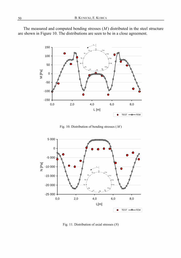
The measured and computed bending stresses (M ) distributed in the steel structure are shown in Figure 10. The distributions are seen to be in a close agreement.
-150
-100
-50
0
50
100
150
0,0 2,0 4,0 6,0 8,0
L [m]
M [P
a]
TEST FEM
Fig. 10. Distribution of bending stresses (M )
-25 000
-20 000
-15 000
-10 000
-5 000
0
5 000
0,0 2,0 4,0 6,0 8,0
L[m]
N [P
a]
TEST FEM
Fig. 11. Distribution of axial stresses (N)

Full-scale laboratory tests and FEM analysis of corrugated steel culverts
51
The measured and computed axial stresses (N ) distributed in the steel structure are shown in Figure 11. The axial stresses predicted are not in a good agreement with the values measured, being significantly higher.
The measured and computed displacements in the steel structure are listed in Table 6. The displacements in selected points are seen to be in a close agreement. The differ-ence between test and FEM analysis is 0.11 mm in the case of vertical displacement and 0.08 mm in the case of horizontal displacements (gauges No. D3).
Table 6. Comparison of displacement in selected points [mm] Point D1 D2 D3
Test 0.95 –2.33 1.03 FEM 0.95 –2.22 0.95
The measured and computed earth pressures in the soil are listed in Table 7. The
earth pressures in selected points are seen to be in a close agreement.
Table 7. Comparison of earth pressure [kPa] Point 1 2 3 4 5 6 7 8 11 13
Test 52.7 51.6 0.1 32.1 27.1 21.4 26.6 31.6 26.7 50.3 FEM 108.7 108.7 0.0 58.8 58.8 88.4 88.4 65.6 26.6 65.6
Fig. 12. Displacement Fig. 13. Von Mises
Fig. 14. Sigma X Fig. 15. Sigma Y

B. KUNECKI, E. KUBICA 52
Cosmos/M system allows us to present several results in graphical form. Displace-ment distribution and deformation are shown in Figure 12. Normal stresses in the x-di-rection are presented in Figure 14, and normal stresses in the y-direction are shown in Figure 15. The von Mises stress (σvon) component is calculated from the stress compo-nents as shown below [7]:
,)](3)()()[( 22222221
von yzxzxyzyzxyx τττσσσσσσσ +++−+−+−= (3)
where: iσ – normal stresses (i – the x, y, z directions),
yxτ – shear stress in the x–y plane,
zxτ – shear stress in the x–z plane,
zyτ – shear stress in the y–z plane.
8. Conclusion
The comparative study indicates that the numerical culvert’s displacements and empirical measurements are almost equal. This means that a stiffness of whole soil–structure system and the finite elements for to modelling were wisely selected. The same correspondence appeared in the case of bending stresses in steel structure.
The axial stresses in the structure are not in a good agreement with numerical and empirical values. The numerical values are significantly higher. Numerical modelling of contact surface between steel shell and soil should be changed. The solution to the problem would be using contact elements like GAP type or applying a springs with specific stiffness between soil and structure.
Stiffness of retaining walls significantly influences distribution of stresses in soil and culvert structure as well (both qualitative and quantitative).
References
[1] Kunecki B., Kubica E.: Experimental identification of load distribution in steel culverts, Research report no. 81/30, pp. 103, Wrocław University of Technology, Institute of Building Engineering, Wrocław, 2002.
[2] Kunecki B. et al.: Report from the investigation on the Multiplate culverts and Helcore and DV/Optima tubes, Report no. IBDiM-TW 26999/W-374, Road and Bridge Research Institute, Wrocław, 1999.
[3] Korusiewicz L., Kunecki B.: Experimental and numerical analysis of internal forces in steel culverts of the multiplate type, The 7th International Conference “Shell Structures, Theory and Application” Gdańsk, October 2002, pp. 137.
[4] Vaslestad J.: Long-term behaviour of flexible large-span culverts, Publication no. 74, Norwegian Public Road Administration, Oslo, 1994, pp. 33.

Full-scale laboratory tests and FEM analysis of corrugated steel culverts
53
[5] Vaslestad J.: Soil structures interaction of buried culverts, Department of Civil Engineer-ing, the Norwegian Institute of Technology, 1990.
[6] Vaslestad J., Madaj A., Janusz L., Bednarek B.: Field measurements of an old brick cul-vert sliplined with a corrugated steel culvert, Transportation Research Board, Washington, 2004.
[7] Rusiński E.: Finite Elements Method – Cosmos/M system, Publication of Transport and Communication, Warsaw, 1994.
[8] Konderla P., Kasprzak T.: Computer methods in elasticity theory. Part one. Finite Ele-ments Method, Dolnośląskie Wydawnictwo Edukacyjne, Wrocław, 1997.
[9] Byrne P.M., Srithar T., Kern C.B.: Field measurements and analysis of large-diameter flexible culvert, Canadian Geotechnical Journal, 1993, Vol. 30, Canada.
[10] Polish Standard: PN-88/ B-02014 – Action on building structures – Soil loading. [11] Polish Standard: PN-81/ B-03020 – Building soils – Foundation bases. Static calculation
and design. [12] Multipel Trummo: Catalog - AROT ViaCon.
Laboratoryjne badania w pełnej skali i analiza MES stalowych przepustów z blachy falistej pod normowym obciążeniem kolejowym
W roku 1998 w Instytucie Badawczym Dróg i Mostów, Filia Wrocław, przeprowadzono pełnowymiarowe badania modelowe przepustu typu GL4 wykonanego w technologii multi-plate. Przedmiotowe badania zrealizowano na zlecenie norweskiego producenta przepustów firmy ViaCon, który dostarczył materiał do badań. Zaprezentowano sposób zamontowania konstrukcji na specjalnie przygotowanym stanowisku badawczym. Podczas badań wykonano wiele obciążeń statycznych oraz dynamicznych, którym towarzyszył pomiar takich wielkości fizycznych jak: odkształcenia, przemieszczenia i napór gruntu na powierzchnie przepustu w charakterystycznych punktach konstrukcji. Przedstawiono sposób montażu czujników na-poru gruntu (presjometrów) wokół powłoki przepustu.
Normowe obciążenie kolejowe (według normy europejskiej UIC 71) zostało zamodelowane przez zastosowanie sztywnej płyty przenoszącej obciążenia z siłowników na grunt.
Badania przeprowadzono dla różnych wysokości naziomu (1,0 m; 0,8 m; 0,6 m; 0,3 m). Ze względu na dużą ilość otrzymanych wyników zaprezentowano jedynie wyniki dla naziomu 0,8 m otrzymane przy obciążeniu statycznym.
Używając programu Cosmos/M, stworzono model numeryczny stanowiska badawczego i konstrukcji przepustu. Na wykresach i w tabelach porównano wyniki empiryczne z wynikami otrzymanymi metodą elementów skończonych.
Z analiz porównawczych wynika zadawalająca zbieżność ugięć powłoki przepustu. Ozna-cza to, że sztywności całego układu grunt–przepust oraz rodzaje użytych elementów zostały właściwie dobrane. Równie zbieżny jest rozkład naprężeń zginających w powłoce przepustu. Naprężenia ściskające mierzone na powierzchni przepustu zachowują jedynie charakter roz-kładu wyznaczonego numerycznie. Należy zastanowić się nad innym sposobem zamodelowa-nia powierzchni kontaktu między gruntem a powłoką przepustu. Sugeruje się zastosowanie elementów kontaktowych (np. typu GAP) lub zastosowanie między przepustem a gruntem sprężyn o określonej sztywności.

B. KUNECKI, E. KUBICA 54
Zauważono bardzo duży wpływ sztywności ścian oporowych na jakościowy i ilościowy rozkład naprężeń zarówno w gruncie, jak i w powłoce przepustu.
ARCHIVES OF CIVIL AND MECHANICAL ENGINEERING
Vol. IV 2004 No. 4
Application of fuzzy sets to determining non-monotone behaviour of the tool life
M. MIERNIK Wrocław University of Technology, Wybrzeże Wyspiańskiego 27, 50-370 Wrocław
The article is an attempt at showing how the theory of fuzzy sets may be used in explaining non-monotone behaviour of the tool-life function. The results obtained in orthogonal turning of Stellite cobalt alloys served as a basis for presenting rules underlying the so-called areas of undetermined chip formation and for determining local extrema of the function. The fuzzy set theory is presented to the extent that is capable of explaining the observed bifurcation between two branches of the function.
Keywords: cutting, cobalt alloys, tool wear, fuzzy sets
1. Non-monotone behaviour of the tool-life function
Among many factors affecting the tool life, the cutting speed is the most important. The well-known formula established firstly by Taylor [1] in 1907 states that
sc
t
vCT = , (1)
where T is the time that is needed to develop a flank wear land of certain dimensions, Ct is the so-called material constant, vc is the cutting speed and s is an experimentally determined exponent dependent on cutting conditions.
Equation (1) gives T as a globally monotone hyperbolic function of the cutting speed vc. Precise studies performed by Podurayev [2] have shown, however, that T be-comes a non-monotone function of vc for higher cutting speeds. The phenomenon has been observed in cutting difficult-to-machine materials as well as steels.
Many attempts have been made to find such a generalized relationship T = f (vc) that would be in a full agreement with physical features of the edge wear process. No such function has been found until now for an arbitrary combination of the tool and the part materials and the wide range of cutting speed.
The non-monotone property of the T = f (vc) relationship is frequently shown as in Figure 1. The Taylor formula (1) is then considered as generally valid but particular segments of the graph have different values of constant Ct and exponent s. According to Podurayev, discontinuities in the Ct and s are due to some abrupt changes in the machining capabilities of tools involved.
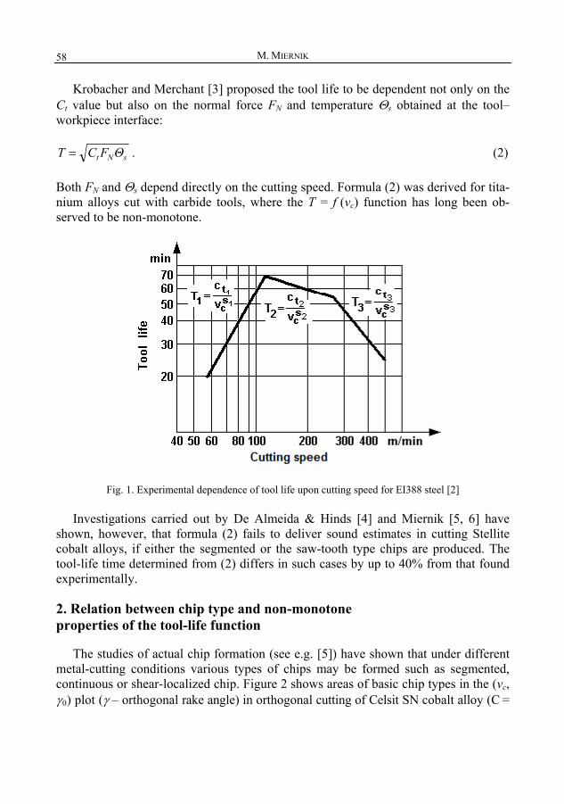
M. MIERNIK 58
Krobacher and Merchant [3] proposed the tool life to be dependent not only on the Ct value but also on the normal force FN and temperature Θs obtained at the tool–workpiece interface:
sNt ΘFCT = . (2)
Both FN and Θs depend directly on the cutting speed. Formula (2) was derived for tita-nium alloys cut with carbide tools, where the T = f (vc) function has long been ob-served to be non-monotone.
Fig. 1. Experimental dependence of tool life upon cutting speed for EI388 steel [2]
Investigations carried out by De Almeida & Hinds [4] and Miernik [5, 6] have shown, however, that formula (2) fails to deliver sound estimates in cutting Stellite cobalt alloys, if either the segmented or the saw-tooth type chips are produced. The tool-life time determined from (2) differs in such cases by up to 40% from that found experimentally.
2. Relation between chip type and non-monotone properties of the tool-life function
The studies of actual chip formation (see e.g. [5]) have shown that under different metal-cutting conditions various types of chips may be formed such as segmented, continuous or shear-localized chip. Figure 2 shows areas of basic chip types in the (vc, γ0) plot (γ – orthogonal rake angle) in orthogonal cutting of Celsit SN cobalt alloy (C =

Application of fuzzy sets to determining behaviour of tool life
59
2.1%, Co = 56%, W = 14%, Cr = 25%; HRC = 51–54). The areas occupied by a given chip type do not have the borders clearly defined. Even under fixed cutting conditions the border areas must be regarded as those where mechanics of chip for-mation is somehow disturbed, which in turn finds its reflection in dependent variables of the cutting process being abruptly changed. Those sets of cutting conditions which give rise to abnormal chip formation have been termed as “areas of undetermined chip formation” (AUCF) and may be considered to be fuzzy sets. This is why the basic chip types in Figure 2 are separated not by lines but by hatched zones of non-zero width.
Various cutting indexes such as shear angle Φ, shear strain γsh and shear strain rate γsh or normal pressure δN acting on the edge have been found to exhibit irregular be-haviour within the AUCF, and derivatives of those indexes with respect to the shear angle have been shown to be functions with singularities [7].
Fig. 2. Areas of occurrence of basic chip forms in cutting Celsit SN cobalt alloy [5]
The AUCF have no clearly defined borders since actual materials deviate signifi-cantly from the ideal model of thermomechanical medium because of their crystalline microstructure, lattice defects, anisotropy of thermoplastic properties, etc. The greater the scatter of local metal properties, the broader the AUCF. Another factor providing the AUCF occurrence are elastic deformations of the tool and machine structure. With all the above arguments gathered, we can say that under AUCF conditions it is impos-sible to formulate definite estimates of the workpiece material machinability or of the tool performance. The available experimental evidence obtained in AUCF machining tests is typical of fuzzy sets.

M. MIERNIK 60
Analysis of the tool wear process, occurring in cutting cobalt alloys with carbide tools, revealed that the normal pressure exerted on the tool face produced by the segmented or shear-localized chips acts not on all the contact area but only on its fraction equal to the thickness of the chip segment [4, 5].
Measurements of cutting forces and characteristic dimensions of the above forms of chip served as a basis for determining actual values of normal pressure δ N acting on the rake face. Results of the analysis (presented in Figure 3) were also used to derive the following modified version of Equation (2):
NNT ΘCT δ= . (3)
Fig. 3. Sudden changes in the value of pressure acting on the rake face [5]
Investigations carried out in study [6] were used for deriving statistically a function T = f (vc) for the Celsit SN cobalt alloy. The function turned out to be non-monotone with two local maxima (Figure 4) which occurred for the cutting speed ranges corre-sponding to the transition between particular chip types.
The above results contradict the Podurayev hypothesis concerning the non-mono-tone behaviour of T =f (vc) resulting from an abrupt change in machining capabilities of the cutting edge (i.e. in material constant values in formula (1)). There is no obvi-ously known physical evidence to support such a statement. It is a sudden shift in thermomechanical behaviour of strain within the cutting zone arising from small changes in the circumstances of the process that is responsible for the externally visi-ble transformation of chip appearance.

Application of fuzzy sets to determining behaviour of tool life
61
Fig. 4. Experimentally observed non-monotone behaviour
of the tool-life function for Celsit SN cobalt alloy
3. Outline of theory of fuzzy sets
Fuzzy sets assigned a characteristic function which determines whether and to what extent an element possesses a certain common feature. Membership of each element in a given set is determined by that feature. A membership function varying from zero to one must be adopted. A variety of function types are available, smooth and non-smooth, the criterion of choice being simplicity, convenience, speed and efficiency or other qualities.
A fuzzy set is an extension of a classical set. If X is the universal set with elements denoted by x , then a fuzzy set A in X is defined as a set of ordered pairs (µA , x), where µA(x) is called the membership function of x in A . The membership function maps each element of X to a membership value (degree) between 0 and 1. If the degree of membership is µA = 1, then element x is certain to belong to set A; if µA = 0, then ele-ment x is surely out of the set.
If a set of elements x is a finite set of discrete values x1, x2,..., xn, then the fuzzy set may be written as
))((...)()(( 2211 nnAAA xxxxxxA µµµ +++= . (4)
Here the sign “+” does not stand for summation but is merely a separator between individual terms determining the degree of membership at a given point ))(( iiA xxµ .

M. MIERNIK 62
4. Application of fuzzy sets to determining the tool life
We will assume that the existence of two neighbouring chip types (denoted by A and B) within the AUCF over the cutting speed range (vg,...,vk) may be, in accordance to Figure 5, presented in the form:
a) for chip type A µA = 1 for vc ≤ vg, µA = (vc–vg) / (vk–vg) for vg < vc < vk, (5) µA = 0 for vc ≥ vk;
b) for chip type B µB = 0 for vc ≤ vg, µB = (vk–vc) / (vk–vg) for vg < vc < vk, (6) µB = 1 for vc ≥ vk.
The morphogenesis theory rooted in concepts developed by Thom [10, 11, 12] ex-plains the AUCF-related phenomena as a bifurcation of function T = f(vc), i.e. the sudden appearance of an additional pattern of behaviour. Each chip type corresponds to a different pattern of strain variation, which in turn results in different values of pressures δN and contact temperatures Θs.
Fig. 5. Probability of occurrence of basic types of chip within AUCF
Had only the chip type A existed within the AUCF, the tool-life function for cutting speeds vc<vk would have followed the TA=f (vc) course. If the same is said of the B type, then the tool-life function for vc>vg would have been in agreement with TB=f (vc), as shown in Figure 6. However, the AUCF is composed of fuzzy sets A and B and each chip type may be assigned a degree of membership in a given set.
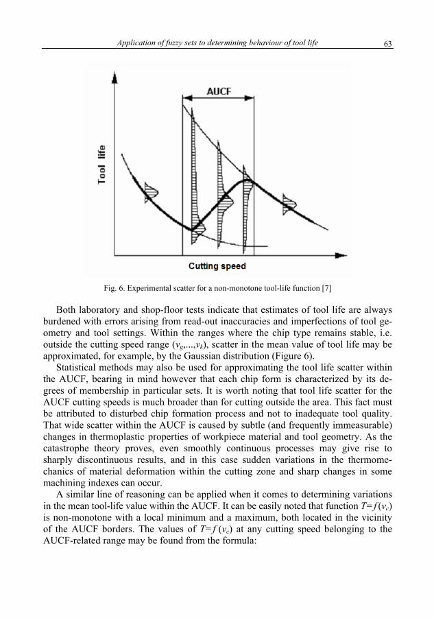
Application of fuzzy sets to determining behaviour of tool life
63
Fig. 6. Experimental scatter for a non-monotone tool-life function [7]
Both laboratory and shop-floor tests indicate that estimates of tool life are always burdened with errors arising from read-out inaccuracies and imperfections of tool ge-ometry and tool settings. Within the ranges where the chip type remains stable, i.e. outside the cutting speed range (vg,...,vk), scatter in the mean value of tool life may be approximated, for example, by the Gaussian distribution (Figure 6).
Statistical methods may also be used for approximating the tool life scatter within the AUCF, bearing in mind however that each chip form is characterized by its de-grees of membership in particular sets. It is worth noting that tool life scatter for the AUCF cutting speeds is much broader than for cutting outside the area. This fact must be attributed to disturbed chip formation process and not to inadequate tool quality. That wide scatter within the AUCF is caused by subtle (and frequently immeasurable) changes in thermoplastic properties of workpiece material and tool geometry. As the catastrophe theory proves, even smoothly continuous processes may give rise to sharply discontinuous results, and in this case sudden variations in the thermome-chanics of material deformation within the cutting zone and sharp changes in some machining indexes can occur.
A similar line of reasoning can be applied when it comes to determining variations in the mean tool-life value within the AUCF. It can be easily noted that function T=f (vc) is non-monotone with a local minimum and a maximum, both located in the vicinity of the AUCF borders. The values of T=f (vc) at any cutting speed belonging to the AUCF-related range may be found from the formula:

M. MIERNIK 64
)))((()))((( ABcBBABcAA TTvTTTvTT −−=−+= µµ , (7)
where µA(vc) and µB(vc) are to be determined according to rules (5) and (6). A discontinuity in the chip formation process occurring within the AUCF can be
observed not only in difficult-to-machine materials but also in more easy-to-machine steels. A continuous chip transforms into a shear-localized chip within the cutting speed range of 150–1000 m/min. This range of speeds is commonly recommended for such tools as coated carbides, ceramics and cubic boron nitride (CBN).
Fig. 7. Bifurcation of the T = f (vc) function within AUCF
Experimental tests serve as a basis for determining an optimum cutting speed vopt ensuring the highest tool life. The life T0 determined statistically for that speed corre-sponds to a local maximum of the tool-life function (Figure 7). If, however, by coinci-dence, thermoplastic properties of machined material and tool geometry start acting together within the AUCF to create conditions promoting a continuous chip instead of shear-localized chip, then quick dulling of a tool will occur after time Tk rather than an expected service life T0. This catastrophic behaviour cannot be attributed to inadequate tool quality and its real cause can be established by meticulous analysis of the chip appearance.
5. Concluding remarks
This study is an attempt to apply the theory of fuzzy sets in the explanation of non-monotone behaviour of the tool-life function and especially the occurrence of local
Application of fuzzy sets to determining behaviour of tool life
65
maxima/minima. The dynamic morphogenesis theory (catastrophe theory) is capable of modelling both continuously progressing processes (quantitative changes) and sud-den jumps from one equilibrium to another (qualitative changes).
Actual machinability tests on Stellite cobalt alloys revealed the existence of the AUCF where the chip formation process undergoes a sudden change. Diffused borders separating particular chip types presented as a function of cutting parameters result from inherent inhomogeneity of machined material and elastic deformability of the tool–machine system. Non-monotonic behaviour of the tool-life function may be at-tributed to the disturbed mechanics of material deformation for those combinations of cutting conditions that give rise to the AUCF occurrence.
References
[1] Taylor F.W.: On the Art of Cutting Metals, Amer. Mach., 1907, Vol. 28. [2] Podurayev V.N.: Cutting of Difficult-to-Machine Materials (in Russian), Vysshaya
Shkola, Moscow, 1974. [3] Krobacher E.J., Merchant M.E.: Basic Factors in Hot Machining of Metals, Trans.
A.S.M.E., 1951, Vol. 94. [4] De Almeida S.M., Hinds B.K.: The Influence of Temperature on the Machinability of
Stellite 6, Proc. 21-th Int. Mech. Tool Des. Res. Conf., Swansea, 1980. [5] Miernik M.: Bases of Cutting Cobalt Alloys (in Polish), Scientific Papers of the Institute
of Machine Building Technology No. 41, Monographs No. 9, Wrocław University of Technology, 1989.
[6] Miernik M.: The Tool Life in the Regions of Undetermined Cutting (in Polish), Scientific Papers of the Institute of Machine Building Technology No. 31, Conferences No. 9, Wro-cław University of Technology, 1986.
[7] Miernik M.: Application of the Catastrophe Theory to the Study on the Chip Formation Process, Eur. J. Mech. Ing., 1992, Vol. 37, 1.
[8] De Almeida S.M., Miernik M., Żebrowski H.: Influence of Microstructure on Chip Formation and Machinability of Some Cobalt Alloys, Material Science and Technology, 1988, Vol. 4.
[9] Cieślak M., Smoluk A.: Fuzzy sets. Image Recognition. Catastrophe Theory (in Polish), PWN, Warszawa, 1988.
[10] Thom R.: Mathematical Models of Morphogenesis, J. Wiley and Sons Inc., New York, 1983.
[11] Poston T., Steward I.: Catastrophe Theory and its Applications, Pitman Publ. Ltd., Lon-don, 1981.
[12] Klamecki B.E.: Castastrophe Theory Model of Chip Formation, Trans. A.S.M.E., J. Eng. for Ind., 1982, Vol. 104, 4.
[13] Von Turkovich B.F.: Influence of Very High Cutting Speed on Chip Formation Mecha-nics, Proc. N.A.M.R.C., 1979, Vol. 7.
[14] Komanduri R. et al.: On the Catastrophic Shear Instability in High-Speed Machining of an AISI 4340 Steel, Trans. A.S.M.E., J. Eng. for Ind., 1982, Vol. 104, 2.

M. MIERNIK 66
Zastosowanie teorii zbiorów rozmytych do analizy niemonotoniczności okresu trwałości ostrza
Przedstawiono przykłady niemonotoniczności funkcji okresu trwałości ostrza podanej przez Taylora. Wykazano doświadczalnie powiązanie między występowaniem podstawowych od-mian wióra (wiór segmentowy, wiór ciągły, wiór piłozębny o zlokalizowanych strefach ścina-nia) a niemonotonicznością funkcji okresu trwałości ostrza skrawającego na przykładzie orto-gonalnego toczenia poprzecznego stopów kobaltowych typu stellit. Zaprezentowano próbę wyjaśnienia przyczyn powstawania niemonotoniczności funkcji okresu trwałości funkcji, opie-rając się na teorii zbiorów rozmytych. Podano reguły obowiązujące w tzw. „obszarach nieokre-ślonego przebiegu formowania wióra”, a dotyczące lokalnych minimów i maksimów funkcji Taylora. Przedstawiono krótki zarys teorii zbiorów rozmytych w ujęciu bifurkacji przebiegu okresu trwałości ostrza, w ujęciu dynamicznej teorii morfologii R. F. Thoma (tzw. teorii kata-strof).

ARCHIVES OF CIVIL AND MECHANICAL ENGINEERING
Vol. IV 2004 No. 4
Analysis of surface roughness profile after its machining in terms of nonlinear dynamics
M. MIERNIK, J. SZYMKOWSKI, M. WIĄCEKWrocław University of Technology, Wybrzeże Wyspiańskiego 25, 50-370 Wrocław
The feed influence on nonlinear changes of the surface roughness after its machining was presented. It was revealed that the derivative of the roughness factor was discontinuous in the function of feed. The roughness profile of a real surface depended on some random factors. Application of fractals (in the form of chaotic attractors) to the analysis of the surface roughness profile after turning was presented. The ef-fect of feed rate and cutting speed on the fractal dimension and the maximum value of Lapunov exponent as well as on the representation characteristics of cutting process in 3D phase surface were evaluated.
Keywords: surface roughness, machining, nonlinear dynamics
1. Introduction
Most goods produced by man are made by machining. This method involves the greatest costs, which encourages us to make a right and wise choice of conditions for such a process. The machining process is named dimensional and surface creating. Construction of a comprehensive machining model that describes genesis of outer layer constitution and allows its comparison to real results is essential.
2. Theoretical model of surface roughness
The first attempt to develop a mathematical model of cutting process was under-taken at the beginning of the twentieth century by Taylor [1] who arrived at statistic-experimental equation for wedge substance. Another model, elaborated by Kaczmarek [2], is based solely on geometric-kinematic mapping (Figure 1).
Making an assumption that nose radius r and the tool cutting edge angles κ and κ1 (κ is main angle and κ1 is minor one) are constant, we can claim that particular cases of mapping depend on feed rate only, and the values of feed, which are consid-ered to be the limits between mapping cases, are called the limit feeds.
The first case of mapping takes place when transverse traces of mapping are formed due to crossing the arch parts of the cutting edge (Figure 1a) – this is arch mapping. This case occurs when:
11 sin2 κ⋅⋅=≤ rff , if κ >κ1, κsin2 ⋅⋅=≤ rff 1 , if κ <κ1. (1)

M. MIERNIK et. al 68
Case r=const, κ=45°, κ1=30°, f-variable
c)
b)
a)
Fig.1. The cases of geometric-kinematic mapping of cutting tool on specimen

Analysis of surface roughness profile after its machining
69
The second case of mapping (Figure 1b) occurs when transverse traces of mapping appear as a result of crossing the arch and straight-line parts of cutting edge and is called the arch–straight-line mapping.
This case takes place for
1
12
1 sin2
sin2sin2
κ
κκ
κ⎟⎠⎞
⎜⎝⎛ +
⋅⋅<<⋅⋅ rfr , if κ >κ1,
(2)
κ
κκ
κsin
2sin
2sin2
12 ⎟⎠⎞
⎜⎝⎛ +
⋅⋅<<⋅⋅ rfr , if κ <κ1.
In the third case (Figure 1c), the transverse traces of mapping appear as a result of crossing straight-line parts of cutting edge. This is the straight-line mapping case which takes place for:
1
12
sin2
sin2
κ
κκ⎟⎠⎞
⎜⎝⎛ +
⋅⋅≥ rf , if κ >κ1,
(3)
κ
κκ
sin2
sin2
12 ⎟⎠⎞
⎜⎝⎛ +
⋅⋅≥ rf , if κ <κ1. .
Based on the theoretical model of the roughness described above it was possible to plot the curve representing the theoretical roughness Rzt (Figure 2).
Fig. 2. Theoretical roughness Rzt versus log f for I, II and III cases of mapping

M. MIERNIK et. al 70
Theoretical surface roughness Rzt and feed limits are listed in the Table. Table. Theoretical surface roughness
Rzt
2245.0 frr −−⎟⎠
⎞⎜⎝
⎛⋅⋅+
⎟⎟⎠
⎞⎜⎜⎝
⎛−⋅−
2sin2
1sin2
sin22sin
12
11
1
κ
κκ
κ
r
fr
f
( )
( ) ⎥⎦
⎤⎢⎣
⎡−
++
×
−+
1sin
sinsin
1sin
sinsin
1
1
1
1
κκκκ
κκκκf
For κ >κ1
Feed
f < f1=2r sinκ1
f1<f<f2
1
12
2 sin2
sin2
κ
κκ⎟⎠⎞
⎜⎝⎛ +
=≥ rff
Symbol Case of mapping I II III
Symbol
For κ <κ1
Feed f< f1=2r sinκ
f1<f<f2
κ
κκ
sin2
sin2
12
2
⎟⎠⎞
⎜⎝⎛ +
=≥ rff
Rzt2245.0 frr −−
⎟⎠⎞
⎜⎝⎛⋅⋅+
⎟⎟⎠
⎞⎜⎜⎝
⎛−
⋅⋅−
2sin2
1sin2
sin22sin
2 κ
κκ
κ
r
fr
f ( )
( ) ⎥⎦
⎤⎢⎣
⎡−
++
×
−+
−
1sin
sinsin
1sin
sinsin
1
1
1
1
κκκκ
κκκκf
The curve in Figure 3 represents geometric-kinematic dependences only. Thus, physical and chemical phenomena in workpiece cutting such as: machine tool proper-ties, edge design, lubricant influence and tool wear are not taken into account.
Fig. 3. Roughness function versus feed
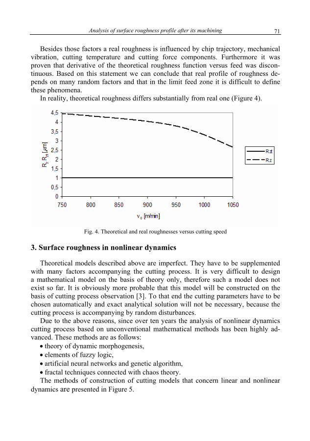
Analysis of surface roughness profile after its machining
71
Besides those factors a real roughness is influenced by chip trajectory, mechanical vibration, cutting temperature and cutting force components. Furthermore it was proven that derivative of the theoretical roughness function versus feed was discon-tinuous. Based on this statement we can conclude that real profile of roughness de-pends on many random factors and that in the limit feed zone it is difficult to define these phenomena.
In reality, theoretical roughness differs substantially from real one (Figure 4).
Fig. 4. Theoretical and real roughnesses versus cutting speed
3. Surface roughness in nonlinear dynamics
Theoretical models described above are imperfect. They have to be supplemented with many factors accompanying the cutting process. It is very difficult to design a mathematical model on the basis of theory only, therefore such a model does not exist so far. It is obviously more probable that this model will be constructed on the basis of cutting process observation [3]. To that end the cutting parameters have to be chosen automatically and exact analytical solution will not be necessary, because the cutting process is accompanying by random disturbances.
Due to the above reasons, since over ten years the analysis of nonlinear dynamics cutting process based on unconventional mathematical methods has been highly ad-vanced. These methods are as follows:
• theory of dynamic morphogenesis, • elements of fuzzy logic, • artificial neural networks and genetic algorithm, • fractal techniques connected with chaos theory. The methods of construction of cutting models that concern linear and nonlinear
dynamics are presented in Figure 5.

M. MIERNIK et. al 72
Theoryof Cutting
Experiment
FuzzyLogic
NeuralNetworks
GeneticAlgorithms
Chaos ResearchFractals
CatastropheTheory
Modelof cutting
LinearDynamics
NonlinearDynamics
Fig. 5. The methods of modeling the cutting process [5]
Up to now fractal analysis in connection with Lapunov’s exponent (λ) monitoring has been the most often used techniques. The exponent (λ) represents a number of valuable information about both the nature of a cutting process and surface subjected to cutting and can be calculated from the expression:
)0()(
limlim0
i
i
ti tt
εε
λε→∞→
= ; i=1,..., dl, (4)
where: λi – calculated exponent for phase space of the i-th direction, dl – local dimension of attractor, t – time, εi (0) – location of an initial trajectory, εi (t) – trajectory location after time t.
The analysis of Lapunov’s exponent consists in choosing its biggest value and de-termining its plus/minus sign. Positive sign (λ > 0) denotes the condition at which

Analysis of surface roughness profile after its machining
73
a c
n for the purpose of cognition.
a)
haotic system exists. The fractal analysis allows creating the so-called chaotic at-tractors and determining fractal dimension. Characteristics of these both factors change together with the cutting parameters.
In Figure 6, the attractors for regular elements are presented. They have no con-nection with nonlinear dynamics, but are show
b)
c)
Fig. 6. Geometrically regular objects and their attractors
4. Experiment conditions

M. MIERNIK et. al 74
The purpose of the experiments was to collect an indispensable data in the form of surfaces of alloy cast-iron workpiece machined by turning in a wide range of cutting par
alues of the greatest Lapunov’s exponent were bigger than zero which suggested that the surfaces investigated had a chaotic character.
ameters. Cutting tool CSRNR 2525-12 with κ = 75° and κ1 = 15° was used. Inserts SNGN 120408T0202 with PVD coatings and the nose radius r = 0.8 mm were used. Cutting speed was varied in the range of 750–1050 m/min, feed of 0.08–0.24 mm/rev, and depth of 0.5–1 mm. Roughness parameters were measured using Form Talysurf 120L Taylor Hobson device.
5. Results of investigations
In all cases, the calculated v
Chaotic attractors created on the basis of phase delay [4] are presented as irregular loops (one loop corresponds to the feed value defined) in Figure 7b.
Fig. 7. Profile of alloy cast-iron being turned (vc = 900 m/min, f = 0.24 mm/rev, ap = 1 mm) (a),
its chaotic attractor (b)
It has been in the values of roughness parameters, i.e. indirectly with an increase in cutting speed and
ension can be helpful as an additional parameter characterizing the surface being machined.
ered loops on geometrical mapping can be seen which was proven by the experiment [6].
also revealed that fractal dimension decreases together with a decrease
a decrease in feed.
6. Conclusions
1. Fractal dim
2. A decrease in feed is accompanied with an increase in fractal dimension. The concentration of non-ord

Analysis of surface roughness profile after its machining
75
3. Fractal analysis could be helpful in the analysis of surface roughness. 4. Both fuzzy logic elements and neural networks can be fruitful in creating moni-
toring systems for machining in real time (on-line).
[1] Taylor F.W.: On the Art of Cutting Metals. Amer. Mach., 1907, Vol. 28. arek J.: Podstawy obróbki wiórowej, ściernej i erozyjnej, Wydawnictwo Nauko-hniczne, Warszawa, 1970.
i Warszawskiej,
Analskrawaniem w ujęciu dynamiki nieliniowej
eliniowość zmian chropowatości ości jest nieciągła w funkcji po-
ży od czynników losowych. Przed-sta
References
[2] Kaczmwo-Tec
[3] Jemielniak K.: Obróbka skrawaniem, Oficyna Wydawnicza PolitechnikWarszawa, 1998.
[4] Ott E.:, Chaos w układach dynamicznych, Wydawnictwa Naukowo-Techniczne, War-szawa, 1997.
[5] Miernik M.: Skrawalność metali. Metody określania i prognozowania, Oficyna Wy-dawnicza Politechniki Wrocławskiej, Wrocław, 2000.
[6] Broll S., Grzesik W.: Zastosowanie analizy fraktalnej do oceny profilu chropowatości po-wierzchni. Zagadnienia inżynierii powierzchni w obróbce skrawaniem, Międzynarodowe Sympozjum Inżynieria Powierzchni ’99, Wrocław–Szklarska Poręba, 7–9.06.1999.
iza profilu chropowatości powierzchni po obróbce
Przedstawiono analizę wpływu posuwu skrawania na nipowierzchni. Wykazano, że pochodna wskaźnika chropowatsuwu, a profil chropowatości powierzchni rzeczywistej zale
wiono wyniki badań nad zastosowaniem fraktali (chaotycznych atraktorów) do analizy pro-filu chropowatości powierzchni po toczeniu. Oceniono wpływ posuwu i prędkości skrawania na wymiar fraktalny i największy wykładnik Lapunowa oraz na charakter odwzorowania dy-namiki procesu skrawania w trójwymiarowej przestrzeni fazowej.

ARCHIVES OF CIVIL AND MECHANICAL ENGINEERING
Vol. IV 2004 No. 4
Correction of geometrical defects of stamping parts by numerical simulation and design of experiment
E. PAIREL, Y. LEDOUX, R. ARRIEUX, L. TABOUROT, O. INCANDELA Laboratory of Applied Mechanics, University of Savoy, BP 806, 74016 ANNECY Cedex, France
A method of correction and optimization of stamping processes is proposed. The experiment design and finite element methods are interfaced. This is applied in a part showing large springback. After de-termining some important process parameters that affect springback, a fractional factorial experiment de-sign is built and the corresponding numerical simulations are carried out. This enabled us to obtain de-formed meshes which were post-processed in order to measure a virtual part geometry. Linear mathe-matical relations between the part geometry and process parameters are established which allows deter-mining their interactions and their influence on the geometrical shape of parts. Finally those mathematical relations were necessary for establishing correct values of the process parameters which lead to the ex-pected geometry of parts.
Keywords: stamping, design of experiments, finite element method, elastic springback, tool optimization
1. Introduction
With an increasing complexity of product geometry, it is more and more difficult to determine the tool geometry and the process parameters of a deep drawing operation. Furthermore, the designers want to control the geometry of the final product with a precision that requires the compensation for the tool geometry in order to take into account elastic deflections that occur after the operation. Empirical rules combined with costing trial and error method are used to find a right combination of process pa-rameters.
Finite element technique may be used to assist engineers but it often poorly reflects the reality because of an approximate modelling both the process and the material be-haviour. Even in this case, the optimization method is still a trial and error method.
In fact, whatever the technique used to optimize the deep-drawing operation, one is often unable to deal with complex interaction between the factors influencing this op-eration. Optimization of complex parts is then a hazardous procedure that often leads to delay, the lack of quality and costing adjustment of the tool geometry (when it is still possible!) and the process parameters.
Nevertheless the design and optimization of the drawing process must be consid-ered using the finite elements simulation.
This paper proposes an alternative to this (lack of) technique. It shows the interest in the application of the design of experiments to deep-drawing process during the process optimization phase in combination with the finite element simulations. In or-
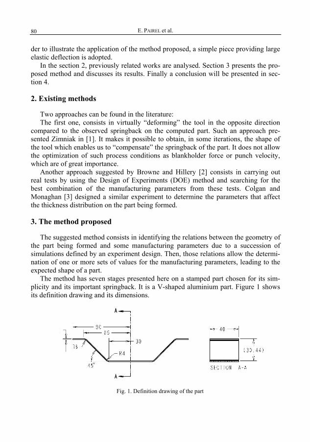
E. PAIREL et al. 80
der to illustrate the application of the method proposed, a simple piece providing large elastic deflection is adopted.
In the section 2, previously related works are analysed. Section 3 presents the pro-posed method and discusses its results. Finally a conclusion will be presented in sec-tion 4.
2. Existing methods
Two approaches can be found in the literature: The first one, consists in virtually “deforming” the tool in the opposite direction
compared to the observed springback on the computed part. Such an approach pre-sented Zimniak in [1]. It makes it possible to obtain, in some iterations, the shape of the tool which enables us to “compensate” the springback of the part. It does not allow the optimization of such process conditions as blankholder force or punch velocity, which are of great importance.
Another approach suggested by Browne and Hillery [2] consists in carrying out real tests by using the Design of Experiments (DOE) method and searching for the best combination of the manufacturing parameters from these tests. Colgan and Monaghan [3] designed a similar experiment to determine the parameters that affect the thickness distribution on the part being formed.
3. The method proposed
The suggested method consists in identifying the relations between the geometry of the part being formed and some manufacturing parameters due to a succession of simulations defined by an experiment design. Then, those relations allow the determi-nation of one or more sets of values for the manufacturing parameters, leading to the expected shape of a part.
The method has seven stages presented here on a stamped part chosen for its sim-plicity and its important springback. It is a V-shaped aluminium part. Figure 1 shows its definition drawing and its dimensions.
Fig. 1. Definition drawing of the part

Correction of geometrical defects of stamping parts by numerical simulation
81
The stamping process is presented in Figure 2 in the “formed part” position. The shape of the part in the tool corresponds to the expected shape and does not take the springback into account.
Fig. 2. Initial stamping process in the final position
3.1. Stage 1: simulation of the initial designed stamping process
The first simulation is carried out with the simple tooling shown in Figure 2 in or-der to check the elastic deflections. The finite-element calculation software Explicit ABAQUS is used. The material used is an 6061 T4 aluminium alloy sheet. The be-haviour law is determined based on tensile tests using an extensometer and an image analysis system for the high-strain levels [4]. It is introduced point by point in the cal-culation software. An elastoplastic isotropic behaviour is assumed. Four layers of 2D rectangular elements allow a part modelling. The element size is smaller in the part ar-eas which will be strongly strained. The contact between the tools and the blank is of the Coulomb type with a friction coefficient f = 0.1 determined by experience.
Taking an isotropic character of aluminium into account, it is decided to realise a planar simulation on half of the profile only (see Figure 3). The simulation of the ini-tial stamping process gives the shape of the part presented in Figure 3.
Fig. 3. Shape of the part obtained by simulation with the initial process
It can be observed that the straight segments of the part keep their rectilinear shape. The defects are essentially dimensional defects: the angle between the bottom and the

E. PAIREL et al. 82
lateral edge is upper than 135°, so an elastic deflection opens the angle after a simple bending operation, as expected; while the angle between the lateral edge and the upper flange is lower than 135°, this means that an elastic deflection closes the angle after a bending–unbending operation on the die radius.
The angles do not have the right values and consequently the height is not enough. So it is decided to characterise those defects by linear and angular parameters (stage 2).
3.2. Stage 2: parametrization of the geometrical defects of the part
Taking into account the observed geometrical defects of the part, it is now neces-sary to characterize them by dimensional parameters which will be measurable on the simulated strained part.
We assume that the profile is composed of straight segments and arcs of circle or of ellipse. These theoretical features will be fitted on the profile of the virtual part, constituting of a set of nodes, in stage 5. This fitting enables us to define the size and location parameters.
It is necessary to redraw the part with the location defects between geometrical features in order to reveal the implicit parameters of the definition drawing (A2 in this example).
Fig. 4. Parameter setting of the part having location defects
Several parameter settings of the geometry are possible. For the part studied, three important geometrical parameters revealing elastic deflections are selected: the two angles A1, A2 and the distance H shown in Figure 4. The radii are not taken into account.
Those parameters will be measured on the simulated part at stage 5.
3.3. Stage 3: searching for the parameters that affect the stamping process
As the previous stage, this one needs also thinking about. It consists in searching for the process parameters that will be able to affect the selected geometry parameters of the part. Moreover, they must be strictly independent of each other: this means that the variation of one of them must be obtained without modification of the others.

Correction of geometrical defects of stamping parts by numerical simulation
83
The selected process parameters are shown in Figure 5. They are as follows: die angle A, die radius R, die width W, punch travel D and blankholder force F.
Those parameters and their variation range are chosen according to the initial simulation and to the observations of their probable influence. Their values are given in Table 1.
Fig. 5. Tool parameters
Table 1. Tested parameters of the stamping process with their fields of variation
Parameter Initial value Low value (–1)
High value (+1)
A: angle of the die 0° 0° 20°
R: radius of the die 6 mm 6 mm 10 mm
W: width of the die 59 mm 52 mm 59 mm
D: depth of the punch 30.44 mm 33 mm 38 mm
F: force of the blankholder 800 N 5 N 1000 N
Finally three equations will be obtained, each representing one geometrical pa-
rameter, i.e. A1, A2 and H, as a function of the five process parameters, A, R, W, D, and F.
3.4. Stage 4: choice of the model and construction of the experiment design
Here we select the first-degree polynomial model which assumes a linear variation of the output from every input:
Y = a0 + a1A' + a2R' + ... + a5 F ' + a12A'R' +... + a45D 'F ' (where Y is A1, A2 or H ).
In this model, the terms Xi, Xj, are the interactions between factors, this means that the effect of one of them Xi, depends on the value of the other one Xj.

E. PAIREL et al. 84
We use a fractional experiment design in order to decrease a number of numerical simulations. For five factors it is necessary to carry out sixteen numerical experiments as shown in Table 2, while for a full factorial experiment design, 32 experiments should be necessary. For every variable, two levels are tested: a low and a high ones defined in Table 1. In Table 2, the levels –1 and +1 correspond respectively to a low value and a high value of the parameter.
Table 2. Experiment design with two levels to test the stamping parameters (a low value of the factor is noted “–1” and a high value “+1”) No. of the experi-ment
Angle of the die A
Radius of the die R
Width of the die W
Depth of the punch
D
Force of the blank-holder F
Result
1 –1 –1 –1 –1 –1 Simulated profile 1
2 –1 –1 –1 +1 +1 Simulated profile 2
3 –1 –1 +1 –1 +1 Simulated profile 3
4 –1 –1 +1 +1 –1 Simulated profile 4
5 –1 +1 –1 –1 +1 Simulated profile 5
6 –1 +1 –1 +1 –1 Simulated profile 6
7 –1 +1 +1 –1 –1 Simulated profile 7
8 –1 +1 +1 +1 +1 Simulated profile 8
Table 2. Experiment design with two levels to test the stamping parameters (a low value of the factor is noted “–1” and a high value “+1”)
No. of the experi-ment
Angle of the die A
Radius of the die R
Width of the die W
Depth of the punch
D
Force of the blank-holder F
Result
9 +1 –1 –1 –1 +1 Simulated profile 9
10 +1 –1 –1 +1 –1 Simulated profile 10
11 +1 –1 +1 –1 –1 Simulated profile 11
12 +1 –1 +1 +1 +1 Simulated profile 12
13 +1 +1 –1 –1 –1 Simulated profile 13
14 +1 +1 –1 +1 +1 Simulated profile 14
15 +1 +1 +1 –1 +1 Simulated profile 15
16 +1 +1 +1 +1 –1 Simulated profile 16
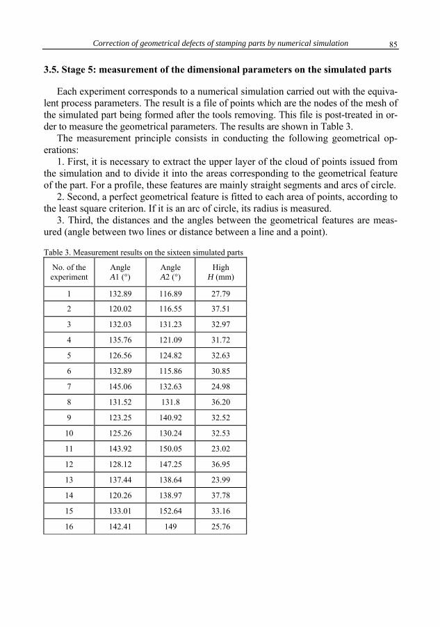
Correction of geometrical defects of stamping parts by numerical simulation
85
3.5. Stage 5: measurement of the dimensional parameters on the simulated parts
Each experiment corresponds to a numerical simulation carried out with the equiva-lent process parameters. The result is a file of points which are the nodes of the mesh of the simulated part being formed after the tools removing. This file is post-treated in or-der to measure the geometrical parameters. The results are shown in Table 3.
The measurement principle consists in conducting the following geometrical op-erations:
1. First, it is necessary to extract the upper layer of the cloud of points issued from the simulation and to divide it into the areas corresponding to the geometrical feature of the part. For a profile, these features are mainly straight segments and arcs of circle.
2. Second, a perfect geometrical feature is fitted to each area of points, according to the least square criterion. If it is an arc of circle, its radius is measured.
3. Third, the distances and the angles between the geometrical features are meas-ured (angle between two lines or distance between a line and a point).
Table 3. Measurement results on the sixteen simulated parts
No. of the experiment
Angle A1 (°)
Angle A2 (°)
High H (mm)
1 132.89 116.89 27.79
2 120.02 116.55 37.51
3 132.03 131.23 32.97
4 135.76 121.09 31.72
5 126.56 124.82 32.63
6 132.89 115.86 30.85
7 145.06 132.63 24.98
8 131.52 131.8 36.20
9 123.25 140.92 32.52
10 125.26 130.24 32.53
11 143.92 150.05 23.02
12 128.12 147.25 36.95
13 137.44 138.64 23.99
14 120.26 138.97 37.78
15 133.01 152.64 33.16
16 142.41 149 25.76

E. PAIREL et al. 86
3.6. Stage 6: calculation and validation the polynomial models Y=f (X)
From the results of the experiment design the coefficients of the polynomial model of every output A1, A2 and H are calculated:
The general method for calculating these coefficients is a multilinear regression. With the sixteen experiments of the fractional experiment design, the following equa-tions are obtained (the most significant effects are in bold type):
A1 = 131.90 – 0.19A' + 1.74R' + 4.58W ' – 2.37D' – 5.05F ' – 0.17A'R' + 0.58A'W ' – 0.32A'D' – 0.5A'F ' – 0.22R'W ' + 0.49R'D' – 0.75R'F ' + 0.35W ' D ' – 0.26W 'F ' + 0.51D'F ' ,
A2 = 133.66 + 9.80A' + 1.88R' + 5.8W ' – 2.32D' + 1.86F ' – 0.53A'R' + 0.47A'W ' + 0.22A'D' – 0.38A'F ' + 0.17RW – 0.68RD – 0.35RF + 0.14WD – 0.59WF + 0.43DF,
H = 31.27 – 0.56A' – 0.60R' – 0.68W ' + 2.39D' + 3.69F ' + 0.06A'R' – 0.31A'W ' + 0.15A'D' + 0.70A'F ' + 0.03R'W ' – 0.41R'D' + 0.58R'F ' – 0.33W ' D' + 0.53W ' F ' – 0.25D'F ' .
A', R', W ' , D' and F' are the standardised variables, respectively corresponding to the die angle A, the die radius R, the die width D, the punch travel W and the tighten-ing force F. They vary from –1 to +1 when the corresponding variable varies from a low value to a high one.
Each of the three models must be validated. For that, three verifications are made: 1. First, the ability of the model to predict the value of the output for any extreme
configuration of the factors, i.e. a configuration such that the factors have the value –1 or the value +1, is checked. These configurations are called the nodes of the study field. There are thirty two (2)5 nodes. Sixteen were already measured in the experi-ment design. For five factors, the adopted models have sixteen independent coeffi-cients, which enables them to pass exactly by the sixteen experimental points of the experiment design. So, this first verification is useless here.
It is thus necessary to test these models on nodes out of the experiment design. One can choose a configuration which, according to the model, gives the minimal or maximum value to the output. In this example, exceptional fact, the configuration given in Table 4 gives, according to the polynomial models, simultaneously the maximum value with the A1and A2 angles and the minimum value for the height H.
One notes that the values predicted by the models deviate from the actual values. The models thus do not seem very precise when the manufacturing parameters have extreme values not tested in the experiment design.
As it is not into the plan, it enables us to test the three models:

Correction of geometrical defects of stamping parts by numerical simulation
87
Table 4: Verification of the models on a particular configuration out of the experiment design No. A' R' W ' D' F ' A1 A2 H
17 1 1 1 –1 –1 Theoretica: 147.1° Theoretic: 152.4°
Theoretic: 21.7 mm
Realb: 142.8° Real: 149.9° Real: 25.4 mm
Deviationc: 4.3° Deviation: 2.5° Deviation: – 3.7 mm
a – obtained with the polynomial model. b – obtained with the numerical simulation by FEM. c – (Y theoretic – Y real).
2. The third verification, consist in checking the ability of the model to predict the value of the output inside the field of study, i.e. when the factors have intermediate values between –1 and +1. For that, the model is tested at the center of the field of study, i.e. when the standard variables are equal to zero and the real variables are equal to their average values.
Table 5: Verification of the models at the center of the field of study No. A' R' W ' D' F ' A1 A2 H
18 0 0 0 0 0 Theoretica: 131.9° Theoretic: 133.7°
Theoretic: 31.3 mm
Realb: 130.2° Real: 132.4° Real: 33.2 mm
Deviationc: 1.7° Deviation: 1.3° Deviation: – 1.9 mm
a – obtained with the polynomial model. b – obtained with the numerical simulation by FEM. c – (Y theoretic – Y real).
One notes again that the models deviate from reality, but the differences are lower than in the preceding extreme configuration.
To improve the precision of the models, it would be necessary to increase the num-ber of tests of the experiment design to enable one to calculate the interactions of the order of 3 and higher and to introduce quadratic terms in order to model the non-line-arity of the phenomena.
In the continuation, the search for the optimal solutions is undertaken with these models by privileging the solutions close to the experimental points of the experiment design in order to limit the error of prediction of the models.
3.7. Stage 7: search for optimal values of stamping process parameters
The objective is to determine the values of the process parameters which allow one to obtain the best values of the part parameters, i.e. as close as possible to the target values: A1 = 135°, A2 = 135° and H = 30.44 mm. The principle consists in minimiz-

E. PAIREL et al. 88
ing a function equal to the sum of the deviations between the theoretical and the de-sired output. In order to keep this sum positive, the deviations are squared:
F = (A1 – 135°)² + (A2 – 135°)² + (H – 30.44)².
This function has several local minima in the field of study defined by the values –1 and +1 of the process parameters. Most of them are shown in Table 6, sorted on the angle A:
Table 6. Several optimal solutions No. of optimal solution
Angle of the die
A' A
Radius of the die
R' R
Width of the die W ' W
Depth of the punch
D' D
Blankholder force F ' F
1 0.35 13.5°
–1 6 mm
0.75 58.1 mm
1 38 mm
–0.91 47 N
2 0.28 12.8°
–1 6 mm
0.74 58.1 mm
0.82 37.5 mm
–0.8 104.5 mm
3 –0.04 9.5°
0.82 9.6 mm
0.24 56.3 mm
0.45 36.6 mm
–0.26 372 N
4 –0.16 8.3°
0.03 8.0 mm
0.50 57.3 mm
–0.06 35.3 mm
–0.11 445 N
5 –0.30 6.9°
–0.21 7.6 mm
0.62 57.7 mm
–0.47 34.3 mm
0.07 540 N
6 –0.44 5.6°
–1 6 mm
0.88 58.6 mm
–0.88 33.3 mm
0.27 638 N
7 –0.53 4.7°
1 10 mm
0.41 56.9 mm
–1 33.0 mm
0.33 669 N
Several selection criteria can be considered to adopt a solution. Because of the pre-cision of the models, it is decided here to select the optimal solution which is the clo-sest to one of the tests of the realised experiment design.
According to this criterion the first solution of Table 6 is taken. This solution has been simulated. The results are shown in Table 7:
Table 7: Verification of the chosen optimal solution for stamping parameters No. A' R' W ' D' F ' A1 A2 H
19 0.35 13.5°
–1 6 mm
0.75 58.1
1 38 mm
–0.9147 N
Theoretica: 135° 135° 30.44 mm
Realb: 133.8° 134.5° 30.4 mm
Deviationc: 1.2° 0.5° 0.4 mm
a – obtained with the polynomial model. b – obtained with the numerical simulation by FEM. c – (Y theoretic – Y real).

Correction of geometrical defects of stamping parts by numerical simulation
89
The simulation of this solution gives the results very close to those predicted, particularly for A2 and H.
4. Conclusion
A method of optimization of stamping processes with numerical simulations has been presented. It uses the fractional experiment designs to obtain linear relations between the geometrical parameters of the formed part and the parameters related to the process of stamping. Those relations allow one to determine the influence of the stamping parameters (tool geometry, blankholder force, punch velocity) on the part geometry [5] and to optimize their values.
Here, it has been applied to an example presenting an important springback and it enables one to determine the shape of the tool and the optimal stamping conditions to compensate for the effects of this springback on simulated parts.
If the results of the numerical simulation are close to reality, the stamping process so designed will give parts of the expected shape.
The models adopted here could be improved by conducting additional tests in order to take the non-linearity of the phenomena and the interactions between stamping parameters of the higher order into account.
This method, under development, will allow one to optimize the design of indus-trial stamping processes by limiting the expensive tests and the corrections in the press shop.
References
[1] Zimniak Z.: Tooling design for sheet metal forming processes compensating springback error, Proceedings of the 6th ESAFORM Conference on Material Forming, V. Brucato (ed.), Italy, April 28–30, 2003.
[2] Browne M.T., Hillery M.T.: Optimising the variables when deep-drawing C.R.1 cups, Journal of Material Processing Technology, 2003, 136, pp. 64–71.
[3] Colgan M., Monaghan J.: Deep drawing process: analysis and experiment, Journal of Material Processing Technology, 2003, 132, pp. 35–41.
[4] Dumoulin S., Tabourot L., Chappuis C., Vacher P., Arrieux R.: Determination of the equivalent stress-equivalent strain relation of a sample of copper in tensile loading, In-ternational Journal of Material Processing Technology, 2003, 133, pp. 79–83.
[5] Pairel E., Ledoux Y., Tabourot L., Arrieux R.: A method to determine relations between process conditions and draw part geometry, XVI International Scientific and Techno-logical Conference on Design and Technology of Drawpieces and Die Stamping, June 14–16, 2004, Poznań, Poland.

E. PAIREL et al. 90
Korekcja geometrycznych defektów wyrobów tłoczonych za pomocą symulacji numerycznej i planowania eksperymentu
Zaproponowano metodę korekcji i optymalizacji procesów tłoczenia. Aby określić sprężynowanie wyrobów charakteryzujących się dużymi odkształceniami, zastosowano sprzężoną metodę planowania eksperymentu i metodę elementów skończonych. Określono istotne parametry wpływające na sprężynowanie, a następnie zastosowano analizę czynnikową i odpowiednie symulacje numeryczne. Wyniki w postaci zdeformowanych siatek zostały użyte do określenia wirtualej geometrii wyrobów. Określono zależności liniowe pomiędzy geometrią wyrobu i parametrami procesu, które umożliwiły ustalenie ich wpływu i wzajemnego oddziaływania na kształt geometryczny wyrobów. Te zależności pozwoliły ustalić poprawne wartości parametrów procesu umożliwiające otrzymanie wyrobów o oczekiwanej geometrii.

ARCHIVES OF CIVIL AND MECHANICAL ENGINEERING
Vol. IV 2004 No. 4
Information about PhD thesis at the Civil Engineering Faculty and the Mechanical Engineering Faculty of Wrocław University of Technology
Title: Nondestructive identification of compression strength of concrete by means of neural networks (in Polish) Nieniszcząca identyfikacja wytrzymałości na ściskanie betonu z wykorzystaniem sztucznych sieci neutronowych
Author: Krzysztof Schabowicz Supervisor: Doctor Jerzy Hoła, Professor of Wrocław University of Technology Promoting Council: Institute of Civil Engineering, Wrocław University of Technology Reviewers:
Professor Zenon Waszczyszyn Professor Mieczysław Kamiński
Date of PhD thesis presentation: February 11th, 2003 PhD thesis is available in Main Library and Scientific Information Centre of WUT The monograph contains: 181 pages, 63 figs, bibliography: 176 items Keywords: nondestructive tests, concrete, compression strength, artificial neural networks
Abstract: Results of experimental and numerical analyses proving that artificial neural networks are suitable for identifying the compression strength of concrete on the basis of its parameters evaluated by nondestructive methods are presented. An overview of the literature on nondestructive methods of evaluating the compression strength of concrete is given. Compression strength identification techniques are compiled and analyzed. Also an overview of the literature on artificial neural network is presented. Neural networks most suitable for the task have been selected.
A database for seven concretes differing in their compression strength and type of aggregate was created on the basis of external and in-house research results. Thus patterns for teaching and testing the selected neural networks were established. The artificial neural networks have proved to be suitable for identifying the compression strength of concrete. Novel methods of identifying the compression strength of concrete on the basis of its parameters evaluated by nondestructive techniques have been developed. The methods have been verified by applying them to real building structures.

Information about PhDs and habilitations 92
Title: Mechanism of strain fracture of materials in quasi-isothermal cutting with one-sided concentrator of stresses (in Polish) Mechanizm lokalizacji odkształceń i pękania materiałów przy quasi-izotermicznym ścinaniu z jednostronnym koncentratorem naprężeń
Author: Grzegorz Chruścielski Supervisor: Professor Edward Stanisław Dzidowski Promoting Council: Mechanical Faculty, Institute of Production Engineering and Auto-mation, Wrocław University of Technology Reviewers:
Professor Jerzy Gronostajski Professor Józef Zasadziński
Date of PhD thesis presentation: September 30th, 2002 PhD thesis is available in Main Library and Scientific Information Centre of WUT The monograph contains: 107 pages, 45 figs, bibliography: 165 items Keywords: chip formation model, mesomechanism, ductile fracture, low SFE materials
Abstract: The process of cutting with one active concentrator of tensions is characterized by its periodicity which causes that the material being separated takes on the shape of chip. This does not occur when two active concentrators of tensions are used for cutting. As is well known, the type of chip results in waste of both energy and tools as well as reliability of machines, espe-cially those being numerically controlled. Therefore, investigations of the mechanisms that determine the type of chip and choice of chip formation process modelling technique are the principle object of present dissertation.
For this reason, the analysis of current state of knowledge of one active concentrator of tension-based process modelling was carried out. It was affirmed that well-known models of continuous chip were not able to generate the criteria of fracture of cutting material and they cannot predict the other types of chips. It was assumed that the main cause of the above was lack of explicit conception of physical modelling of this group of processes. In particular, this concerns the cutting in isothermal conditions, where the most of well-known types of chips are formed, including continuous chip – the least desirable for automatic machining centres.
It was put forward a thesis that further development of modelling of the processes based on one active concentrator of tensions was possible only due to development of a new conception of physical modelling. In oder to support this thesis, a mesoscope conception of modelling of two-concentrators-based processes reported by Dzidowski was applied. This conception is based on structural levels of plastic deformation, especially on the results of dislocation struc-ture evolution leading to deformation localization in isothermal shear bands. Thus it generates new criteria and possibilities for controlling the fully comprehended processes of cutting.
It was proposed the experimentally verified new model of cutting with one active concen-trator of tensions. This model is based on the conception of Dzidowski, but some modifications in specificity (cycle) of processes based on cutting with one active concentrator of stresses are made. Therefore, it can be applied to the description of mechanism and the way of forming different types of chips. In particular, this model is useful for modelling the processes based on separation of thin layers of material by plastic cutting.

Information about PhDs and habilitations 93
Title: Influence of slides on frictional contact in conditions of dry rolling-sliding friction (in Polish) Wpływ poślizgów na sprzężenie cierne w warunkach suchego tarcia toczno-ślizgowego
Author: Zbigniew Ferenc Supervisor: Professor Czesław Koziarski Promoting Council: Institute of Machines Design and Operation, Wrocław University of Technology Reviewers:
Professor Włodzimierz Waligóra Professor Zbigniew Lawrowski
Date of PhD thesis presentation: April 27th, 2004 PhD thesis is available in Main Library and Scientific Information Centre of WUT The monograph contains: 128 pages, 104 figs, bibliography: 133 items Keywords: microslip, kinematic slip
Abstract: The influence of tangent forces on overloads occurring on the contact surfaces of collaborating machine elements and torque transmission instability, deformation continuity and displacements associated with this were presented. The measurements of forces and torque coupled with friction at the strictly set slide values and revolving and linear speeds were carried out. Displacement on the contact surfaces was measured by optical method following completion of force and torque measurements. Temperature on anterior surface at a few chosen parameters of coupling was registered. At the end the results of investigation of cone-form metal samples seizing were presented. Temperature and resistant forces at 15% sliding were measured.

Information about PhDs and habilitations 94
Title: An influence of mechanical stabilisators on the changes in the spine flexibility (in Polish) Wpływ zastosowania stabilizatorów mechanicznych na zmiany podat-ności kręgosłupa
Author: Agnieszka Szust Supervisor: Professor Romuald Będziński Promoting Council: Institute of Machines Design and Operation, Wrocław University of Technology Reviewers:
Professor Jan Marciniak Doctor Mieczysław Szata
Date of PhD thesis presentation: November 19th, 2004 PhD thesis is available in Main Library and Scientific Information Centre of WUT The monograph contains: 210 pages, 203 figs, bibliography: 112 items Keywords: biomechanics of the human spine, overstress, stability, method of the stabilisation Abstract: The monograph deals with the human spine, in particular it analyses of the load of the lumbar and thoracic spines in physiological conditions under functional load and in pathologically destabilised conditions. Experimental examination of the specimens of a natural lumbar spine was carried with the testing machine MTS-Bionix.
The examination consists of: a physiological spine test, a destabilized spine test; a test on a destabilized spine that was restabilized by the systems of implants used in orthopaedic treat-ment of lateral curvatures of the spine. The test carried out on three stabilizing systems made it possible to analyse the response of the lumbar and thoracic spines to flexion/extension and compression.
This experimental analysis is necessary for characterising the factors affecting the spine flexibility.

Information about PhDs and habilitations 95
Title: Wavelet analysis in parametric identification of discrete dynamic sys-tems (in Polish) Analiza falkowa w parametrycznej identyfikacji dyskretnych układów dynamicznych
Author: Magdalena Napiórkowska-Ałykow Supervisor: Professor of Wrocław University of Technology Wojciech Glabisz Promoting Council: Institute of Civil Engineering, Wrocław University of Technology Reviewers:
Professor Jerzy Rakowski, Poznań University of Technology Professor Paweł Śniady, Wrocław University of Technology
Date of PhD thesis presentation: October 20th, 2004 PhD thesis is available in Main Library and Scientific Information Centre of WUT The monograph contains: 150 pages, 59 figs, bibliography: 146 items Keywords: wavelet packet analysis, parametric identification Abstract: The dissertation presents an application of, never used so far, wavelet packet analysis in the parametric identification of discrete dynamic systems. A new algorithm, founded on Walsh packet properties, was developed and applied in solving signal derivatives, which are the basis of the parametric identification of discrete dynamic systems. A new procedure of identification, based on the Haar filter and filtered form of signal derivatives, was developed. This procedure enables reduction of derivative degree. The algorithms were tested in single degree of freedom systems (SDOF) and two degree of freedom systems, which were described by linear and nonlinear equations with constant and variable coefficients.

Information about PhDs and habilitations 96
Title: Usefulness of polymer sulphur composites to the protection of rein-forcement and concrete against corrosion (in Polish) Przydatność polimerowych kompozytów siarkowych do ochrony przed korozją stali zbrojeniowej i betonu
Author: Mariusz Książek Supervisor: Professor of Wrocław University of Technology Jerzy Hoła Promoting Council: Institute of Civil Engineering, Wrocław University of Technology Reviewers:
Professor Lech Czarnecki Professor Mieczysław Kamiński, Wrocław University of Technology
Date of PhD thesis presentation: June 16th, 2004 PhD thesis is available in Main Library and Scientific Information Centre of WUT The monograph contains: 152 pages, 101 figs, bibliography: 137 items Keywords: polymer sulphur composite, surface protection against corrosion, reinforcement, concrete Abstract: This paper presents the results of the experimental research and analyses indicating the usefulness of polymer sulphur composites to the protection of reinforcement and concrete against corrosion. The paper presents the review of the literature, among other things, a select use of polymer sulphur composites in buildings, the methods of the surface protection of rein-forcement and concrete against corrosion and the methods of evaluating a protection layer on these materials. The research deals with the composition of materials and the conditions for their formation. The physical and mechanical properties of polymer sulphur composites were evaluated. After the analysis of the initial results the optimum compositions of polymer com-posites were chosen. The experimental program comprised: adhesion of the composite to smooth and ribbed reinforcement and to a standard mortar and concrete, the loss of the com-posites or reinforcement and ordinary concrete in acid solutions, alkaline and salt solutions and in the water. Parallely the polarization tests were carried out on reinforcement and concrete with or without covering them with polymer sulphur composites. The usefulness of polymer sulphur composites to the surface protection of reinforcement and concrete against corrosion was evaluated.

Information about PhDs and habilitations 97
Title: Modelling and dynamic analysis of steel beam bridges under moving load (in Polish) Modelowanie i analiza dynamiczna belkowych mostów stalowych pod obciążeniem ruchomym
Author: Monika Podwórna Supervisor: Professor Marian Klasztorny Promoting Council: Institute of Civil Engineering, Technical University of Wrocław Reviewers:
Professor Paweł Śniady Doctor Roman Lewandowski
Date of PhD thesis presentation: June 18th, 2003 PhD thesis is available in Main Library and Scientific Information Centre of WUT The monograph contains: 137 pages, 53 figs, 18 tables, bibliography: 42 items Keywords: railway bridge, steel beam bridge, trains, non-linear modelling, dynamic analysis Abstract: The dissertation concerns dynamics of single-track, single-span, steel beam railway bridges carrying high-speed passenger trains. Physically non-linear modelling of the bridge-track-moving train system (MTP) and a computer algorithm for calculating dynamic and quasi-static responses of a bridge to a moving train are developed. The main goal is to derive a design model of the MTP system, i.e. the model with simplifications acceptable from a practical point of view. Dynamic analysis of steel beam bridges loaded with passenger trains moving at velocities of 100–300 km/h has been performed on a series-of-types of bridges.

Information about PhDs and habilitations 98
Title: Deflection of the continuous RC beams under sustained loads
(in Polish) Ugięcia długotrwale obciążonych statycznie niewyznaczalnych belek żelbetowych
Author: Sebastian Toś Supervisor: Professor of Wrocław University of Technology Mariusz Szechiński Promoting Council: Institute of Civil Engineering, Wrocław University of Technology Reviewers:
Professor Tadeusz Godycki-Ćwirko, Gdańsk University of Technology Professor Mieczysław Kamiński, Wrocław University of Technology
Date of PhD thesis presentation: October 13th, 2004 PhD thesis is available in Main Library and Scientific Information Centre of WUT The monograph contains: 134 pages, 187 figs, bibliography: 119 items Keywords: reinforced concrete, continuous beams, long-term deflection Abstract: The dissertation deals with the behaviour of the continuous RC beams under sus-tained loads. Two-span beams of rectangular and T-shaped cross sections were analyzed. The tests were conducted on elements in the uncracked phase and in the phase after cracking.
In order to find the load-carrying capacity of the elements, a disruptive investigation was carried out. Besides the author evaluated the material characteristics of the concrete and the steel: compressive and tensile strength as well as the modulus of elasticity. Simultaneously the rheological behaviour of the concrete used (creep and shrinkage) under the sustained loads was investigated. The concrete samples in the shape of a cylinder were used. The results were given in the form of diagrams and represented by mathematical functions as well.
In theoretical research, the author analyzed present methods of estimating the deflections of RC structures under sustained loads. He assumed that it was possible to estimate the deflection of the RC structure under sustained load by reducing its stiffness in time. The effects of theo-retical analysis were compared with experimental results.

Information about PhDs and habilitations 99
Title: The influence of subsoil vibrations on horizontal pressure of granular material exerted on silo walls (in Polish) Wpływ drgań podłoża gruntowego na poziome parcia materiału sypkiego na ściany silosu
Author: Radosław Tatko Supervisor: Professor of Wrocław Uniwersity of Technology Sylwester Kobielak Promoting Council: Institute of Civil Engineering, Wrocław Uniwersity of Technology Reviewers:
Professor Roman Ciesielski, Cracow University of Technology Professor Mieczysław Kamiński, Wrocław University of Technology
Date of PhD thesis presentation: June 9th, 2004 PhD thesis is available in Main Library and Scientific Information Centre of WUT The monograph contains: 133 pages, 163 figs, bibliography: 66 items Keywords: silo, granular material, subsoil vibrations, horizontal pressure Abstract: The dissertation describes laboratory investigation of steel flat-bottomed silo model filled with sand and subjected to external dynamic loads. The silo was placed on a system of springs, which represents a subsoil. The loads in the form of horizontal impulses were applied to a bottom plate of the silo. Horizontal pressure in time was used for analysing the influence of subsoil vibrations on the distribution of the pressure changes. Basic conclusions: (1) the subsoil vibrations cause two types of changes of the horizontal pressures: constant changes which are observed after completion of model vibrations and cyclic momentary changes; (2) the subsoil vibrations generate a constant increase or constant decrease in pressure.

Information about PhDs and habilitations 100
Title: Application of wavelets in direct methods of structural mechanics (in Polish) Zastosowanie falek w przybliżonych metodach mechaniki budowli
Author: Tomasz Koźbiał Supervisor: Doctor Wojciech Glabisz, Professor of Wrocław University of Technology Promoting Council: Institute of Civil Engineering, Wrocław University of Technology Reviewers:
Doktor Jerzy Rakowski, Professor of Poznań University of Technology Professor Piotr Konderla
Date of PhD thesis presentation: May 12th, 2004 PhD thesis is available in Main Library and Scientific Information Centre of WUT The monograph contains: 91 pages, 46 figs, 9 tables, bibliography: 87 items Keywords: wavelet analysis, direct methods Abstract: The dissertation presents a new, rarely used so far, way of constructing the solutions in the direct methods of structural mechanics which involves wavelet approximations. Discrete and wavelet packet analyses are used in some one- and two-dimensional boundary-value prob-lems analysed by the extended Galerkin and Ritz methods. New adequate algorithms are devel-oped and applied in solving mechanical problems such as bending of beams and plates and stability analysis of beams. The results obtained are compared with the exact solutions or with those from the traditional finite-element method. The techniques of computation of integrals of the products of wavelets and their derivatives (called connection coefficients) for Daubechies wavelet family are proposed.


