UCGE Reports Number 20301 Department of Geomatics Engineering Arctic Sea Ice Freeboard Heights from Satellite Altimetry (URL: http://www.geomatics.ucalgary.ca/graduatetheses) by Vidyavathy Renganathan January 2010
therefore, cannot be extrapolated to interpret sea ice conditions in the open ocean.
Brown and Cote (1992) analyzed the ice thickness data from 1950 to 1989 in the
Canadian Arctic and concluded that (i) the interannual variability of land fast ice
thickness is closely tied to annual and decadal variations in snow depth and, (ii) in
order to separate the thinning trends from inter-annual variability, longer time series
of data from more monitoring stations are needed. Drilling techniques can also be used
to infer the thickness distribution in an ice floe, by creating a probability distribution
function using sufficient number of samples. Eicken and Lange (1989) suggest that a
good representation of the thickness distribution in an ice floe is possible to achieve
even with shorter profiles. Drilling methods have poor spatial and temporal resolution
because they are labor intensive, expensive and are usually carried out in campaigns.
On the other hand, they provide a highly accurate validation data set that is required
for remote sensing data calibration and validation. In situ measurements of physical
properties of snow and ice are also needed in order to convert sea ice freeboard into
sea ice thickness using isostatic equilibrium assumptions (Equation 3.1).
Ground penetrating radar (GPR) GPRs are also widely used to measure the
snow and sea ice thickness by converting the GPR velocities into thickness esti-
21
220˚
220˚230˚
230˚
240˚
240˚
250˚
250˚
260˚
260˚
270˚
270˚
280˚
280˚
290˚
290˚
300˚
300˚
310˚
310˚
60˚ 60˚
65˚ 65˚
70˚ 70˚
75˚ 75˚
80˚ 80˚
85˚ 85˚
Alert
Baker Lake
Cambridge Bay
Coral Harbour
Eureka
Hall Beach
Inuvik
Iqualit
Resoulte
Yellowknife
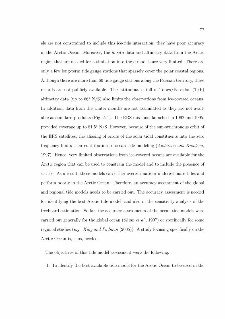
Figure 3.1: The New Arctic Program monitoring stations in the Canada.
mates. This method can provide larger spatial coverage when compared to the drilling
method. However, GPR is a field remote sensing technique. Hence, it has a larger
uncertainty in the ice thickness measurements when compared to the drilling method.
Galley et al. (2009) found good agreement between the GPR measurements and the
physical and dielectric properties of the snow/ice medium.
3.2 Remote Sensing
3.2.1 Submarine
Upward-Looking Sonar (ULS) ULSs are mounted on submarines and used to
measure the sea ice draft (Fig. 3.3). The pressure sensor located in the submarine’s
hull measures the depth of the ULS below sea level. The sonar transducer mounted
on the conning tower of the submarine measures the time taken by the sound beam
to reach target (under-ice topography) and reflect back to the transducer (which can
22
Figure 3.2: The land-fast ice thickness profiles measured at a number of monitoring stations in the Canadian Arctic.Data archived by the Canadian Ice Service.
23
Figure 3.3: A schematic representation of the submarine, sonar beam, and the icecover. The pressure sensor measures the keel depth, D. The height H is the verticaldistance from the pressure sensor to the sonar transducer, mounted on the conningtower at depth DT . ‘r’ and ‘row’ are the ranges to the ice and open water. ‘d’ is themeasured sea ice draft. Source: Rothrock and Wensnahan (2007).
be interpreted as the distance between the ULS and ice bottom surface). These two
measurements are combined to derive the sea ice draft.
Sea ice thickness, t, can then be calculated from the sea ice draft, d, by assuming
isostatic equilibrium, using equation 3.1,
t =ρwd− ρss
ρi
, (3.1)
The snow depth (s) and the densities of water (ρw), ice (ρi) and snow (ρs) are
obtained from in situ measurements or standard values are assumed. The standard
values and the expected uncertainties in each of these parameters are described in
more detail in Chapter 7, section 7.3.
24
ULS mounted on United States Navy submarines have routinely measured the ice
draft in the Arctic Ocean since 1958 (Rothrock et al., 1999). Data from approximately
70 cruises, at least one per year that lasted about 20-40 days, were archived. These
data include measurements of both the winter maximum and the summer minimum
ice draft. Data from 1976-2000 covering about 120,000 km of profiles were made
available to the science community through the National Snow and Ice Data Center
(NSIDC) .
These draft measurements were collected for safe maneuvering of submarines in
ice-covered oceans and were not intended for scientific research. Hence, these data
sets have random spatial and temporal coverage. If these data sets are to be used
in scientific research, knowledge of their quality or an error estimate is essential.
Rothrock and Wensnahan (2007) identified the possible sources of errors in subma-
rine draft measurements, namely measurement precision, errors in identifying open
water, sound speed error, errors due to variable sonar footprint size, uncontrolled
gain and thresholds, difference between analog and digitally recorded data. The mea-
sured pressure is converted into keel depth using an assumed sea water density value,
which introduces additional errors. Rothrock and Wensnahan (2007) report that the
submarine drafts have a tolerable error of ∼ 25 cm averaged over 10’s of kilometers
and, therefore, these data sets can be used to validate observations from spaceborne
techniques.
Submarine drafts were used in a number of studies to estimate the thinning of
Arctic sea ice cover (e.g., Rothrock et al. (1999), Rothrock et al. (2003), Yu et al.
(2004), Zhang et al. (2000), Wadhams and Davis (2000)). Rothrock et al. (1999)
found that the mean ice draft in the Arctic Ocean decreased by ∼ 40% between 1958-
25
1976 and 1993-1997. Wadhams and Davis (2000) found a 43% decrease in mean ice
draft between 1976-1996. Studies attribute the decrease in ice draft to (i) changes in
precipitation, and (ii) increased ice export that is associated with decadal variations
in atmospheric circulation, North Atlantic Oscillation (NAO) and Arctic Oscillation
(AO) (Kwok and Rothrock , 1999).
3.2.2 Airborne
Electromagnetic Induction The Electromagnetic Induction (EMI) sounding tech-
nique has been used, since 1990, to collect sea ice thickness measurements in the Arctic
and the Antarctic (Kovacs and Holladay (1990), Haas (2004), Eicken et al. (2001)).
The EMI instrument can be used to collect both ground-based and airborne data.
However, they can yield only limited spatial and temporal resolution compared to the
spaceborne techniques. Shipborne measurements are possible but are limited by the
fact that ships cannot penetrate through the thickest ice regions. The EMI technique
is based on measuring the sub-surface mean electrical conductivity. Because of the
strong contrast in electrical conductivity between sea ice layer, 0 ∼ 50 mSm−1 (milli-
siemens per metre) and underlying cold sea water, ∼ 2500 mSm−1, the EMI can
successfully distinguish between the two mediums and measure the sea ice thickness
(Haas , 2003). The transmitter coil creates a primary electromagnetic field that in-
duces eddy currents at the ice-ocean interface (see Fig. 3.4). As a result, a secondary
electromagnetic field is generated. The receiver coil then measures the strength and
phase of the secondary field which is dependent on the thickness of sea ice. Thick ice
produces a weak secondary field, while thin ice produces a strong secondary field.
26
Figure 3.4: The principle of Electromagnetic Induction ice thickness sounding.Source: Haas (2003). The transmitter coil generates the primary field that induceseddy currents at the ice-ocean interface. Consequently, a secondary field is generated.The receiver coil measures the amplitude and phase of the secondary field.
The EMI method has an accuracy of ∼ 10 cm over level ice, estimated from the
comparisons with drilling measurements (Haas, 2003). It has a much poorer accuracy
over pressure ridges, because the ice thickness is underestimated in those regions. The
measurements are averaged over a certain footprint area that is approximately equal
to the distance between the sensor and the water surface. Hence, over ridge keels,
the receiver records mixed signals from the narrow ridge keel and the adjacent sea
water, thus underestimating the ice thickness. In Antarctica, the gap layer below
the superimposed ice also causes underestimation of ice thickness (Haas, 2003). If
the height of the sensor system above the sea level is known, then freeboard can be
derived using isostatic equilibrium assumptions (Equation 3.1). These independent
EMI freeboard estimates can be used as validation data for freeboard estimates from
satellite altimetry.
27
Figure 3.5: Mean ice thickness measured from an airborne laser altimeter near Green-land from mid to late June 1998. Source: Hvidegaard and Forsberg (2002).
Haas et al. (2008) analyzed airborne-EMI measurements made from helicopters
during late summers of 2001, 2004 and 2007 over the Transpolar Drift. They found
an ongoing reduction of up to 44% in the mean ice thickness near the North Pole
region and suggested that the main reason for this reduction is due to a regime shift
in sea ice from multi-year ice to second-year ice to first-year ice.
Laser Altimetry Sea ice freeboards can be derived using airborne laser altimetry
techniques. Hvidegaard and Forsberg (2002) analyzed data collected with an Optech
501SX laser altimeter during the airborne gravity campaigns in 1998 over the polar
seas off northern Greenland. Figure 3.5 shows the ice thickness calculated from the
measured freeboards. Hvidegaard and Forsberg (2002) estimated an accuracy of ∼15
cm for the derived freeboards and a thickness accuracy of ∼1 m. The laser altime-
ter operates at a wavelength of 904 nm and has a footprint size of less than 1 m.
28
GPS (Global Positioning System) receivers onboard provides precise positioning. A
laser altimetry system measures the surface elevation which is reduced to sea ice free-
board by combining the elevations with a regional geoid model (Forsberg et al., 2000).
Sea ice freeboard can be converted into sea ice thickness using isostatic equilibrium
assumptions (Equation 3.2).
K = 1 +ρihi + ρshs
hi(ρw − ρi) + hs(ρw − ρs)(3.2)
where K is the conversion factor, h and ρ are the thickness and density values
respectively, for ice (i), snow (s) and water (w). The standard values and the expected
uncertainties in each of these parameters are described in more detail in Chapter 7,
section 7.3.
Major error sources were identified as snow loading (leads to an overestimation of
thickness), lack of open water regions (leads to underestimation of thickness) and, er-
rors in the freeboard to thickness conversion factor (on the order of ∼30 cm, Wadhams
et al. (1992).
Varnai and Cahalan (2007) describe the potential of offbeam lidar techniques to
provide snow and ice thickness measurements. The method is based on, “observing
the horizontal spread of lidar pulses: The bright halo observed around an illuminated
spot extends farther out in thicker layers because photons can travel longer without
escaping through the bottom” (Voss and Schoonmaker (1992), Fig. 3.2.2). This
principle was already used in many applications, e.g., to measure thickness of clouds
(Polonsky et al., 2005). Sea ice halos are usually larger because sea ice is much
thicker than snow and snow halos are brighter because snow has more scatterers in
the medium (Varnai and Cahalan, 2007). The authors report that for snow and
29
Figure 3.6: A schematic representation of the airborne sea ice measurements usingoffbeam lidars Source: Varnai and Cahalan (2007).
sea ice thickness (< 30 cm and 3 m, respectively) the uncertainties in the thickness
retrievals are ∼ 10%.
3.2.3 Spaceborne
Passive Microwave The first global views of the sea ice cover was made possi-
ble by the development of spaceborne measurement techniques. Passive microwave
sensors have been used to monitor the sea ice extent, area, concentration and ve-
locity since 1978. Advanced Very High Resolution Radiometer (AVHRR), Scanning
Multichannel Microwave Radiometer (SMMR) and Special Sensor Microwave/Imager
(SSM/I) have been widely used to determine the trends in sea ice extent (Fig. 1.1,
Gloersen et al. (1999), Parkinson et al. (1999), Comiso (2002), Comiso et al. (2003)
and Comiso and Parkinson (2008)). Agnew et al. (2008) used AMSR-E enhanced
resolution data from 2002-2007 to estimate the daily sea ice area fluxes between the
Canadian Arctic Archipelago and the Arctic Ocean and Baffin Bay. Cavalieri and
Parkinson (2008) analyzed 28 years of Antarctic sea ice extent derived from SSM/I
and SMMR and found that the total Antarctic sea ice extent trend increased slightly
30
from approximately 1.0 ± 0.4% per decade. Kwok (2008) used AMSR-E data to
reliably retrieve sea ice motion in the Arctic. He states that this sensor has improved
spatial resolutions and lower sensitivity to atmospheric moisture which resolved a
number of previous issues with the sea ice motion retrieval process.
Gloersen et al. (1999) reported a global sea ice extent decrease by 0.01±0.003 ×
106 km2 per decade and decrease in areal coverage as 0.009±0.002×10⁶ km2. Parkin-
son et al. (1999) analyzed a 18.2 year record of Arctic sea ice extent from SSM/I
(1978-96) and found seasonal, regional, and interannual variabilities with an overall
decreasing trend of 34300 km2yr−1. It is important to note that in order to compre-
hensively study the changes in sea ice cover due to climate change and variability,
change in sea ice volume (both area and thickness) must be analyzed.
Sea ice velocities can also be derived from SSM/I. Alexandrov et al. (2000) stud-
ied the sea ice exchange between Laptev Sea and the Arctic Ocean using ice drifts
from SSM/I, imaging side-looking radar and a dynamic-thermodynamic model. Kwok
(2000) examined the sea ice motion associated with NAO using 18-years of SSM/I
and buoy data. Variation in the sea level pressure due to NAO results in wind forc-
ing, which in turn changes the sea ice circulation in the Arctic Ocean. Consequently,
ice flux, ice extent, and ice thickness distribution are affected. Kwok and Rothrock
(1999) and Kwok et al. (2004a) identified significant correlation between sea ice area
flux through the Fram strait and the NAO index.
Because of its capability to monitor during day/night and at almost all-weather
conditions at global scale with high temporal resolution (∼ daily), passive microwave
sensors are the primary tool that provides relatively long historical record of sea ice
31
conditions in the Arctic and Antarctic. SSM/I data have a spatial resolution of about
25 km× 25 km. These data are freely available through NSIDC and have been used
in a number of studies to analyze the spatial and temporal variations in sea ice cover
at global scales. Fig. 3.7 shows the Arctic sea ice extent which was ∼ 15.14 million
square kilometers on February 28, 2009, the day it reached a winter maximum for
the year (source: NSIDC). The maximum extent was reported to be 720,000 square
kilometers less than the 1979-2000 average (NSIDC).
Synthetic Aperture Radar Synthetic Aperture Radar (SAR) is a spaceborne
imaging radar system onboard RADARSAT–1/2, ERS–1/2, Envisat ASAR, and
TerraSAR-X satellites among others. SAR backscatter data have been used to dis-
criminate between various features, such as multi-year ice (MYI), first-year ice (FYI),
and open water or leads (Kwok et al. (2004b), Melling (1998)). Figure 3.8 shows MYI
characterized by its brighter tone and rough texture (region A), old ice floes identi-
fied by bright round shapes (regions C and D), open water distinguished by its dark
tone (region E) and pressure ridges identified by bright linear features (region F).
Sea ice type information obtained from SAR backscatter data can be used to inter-
pret radar/laser altimetry waveforms. Therefore, the laser altimeter onboard ICESat
(which delivers both the waveform and ellipsoidal height for every footprint) has the
potential to provide both thickness and sea ice type information.
Bogdanov et al. (2007) describe a number of algorithms to retrieve sea ice pa-
rameters from SAR data, including supervised and unsupervised sea ice classification
and sea ice concentration. SAR data have also been used to study the sea ice mo-
tion and deformation in the Arctic Ocean (Kwok and Cunningham (2002), Kwok
(2004)). Barber et al. (1998) identified the different thermodynamic phases in the
32
Figure 3.7: Arctic sea ice extent on February 28, 2009, the date of the annual max-imum. The orange line shows the 1979 to 2000 median extent for that day. Credit:National Snow and Ice Data Center.
33
Figure 3.8: RADARSAT SAR image showing different sea ice types in the EastSiberian Sea. A – multi-year ice; B – first-year ice; C and D – floes of old ice; E –leads. Source: Alexandrov et al. (2007).
seasonal evolution of radar backscatter: fall freeze up, winter, early melt, melt onset
and advanced melt. Changes in backscatter for snow-covered FYI and MYI during
these periods are shown in Barber et al. (2001). Yackel et al. (2001) evaluated the
potential of time-series RADARSAT-SAR data to detect the melt onset on landfast
FYI. Wadhams et al. (1991) found a positive correlation between SAR backscatter
level and ice drafts (measured by sonar), although the processes that influence the
backscatter are not directly related to thickness. They reported that only 46% of the
backscatter variances are explained by draft variations. In summary, SAR systems
are an important tool for monitoring the geophysical state of the sea ice.
34
3.3 Sea Ice Modeling
Coupled ice-ocean models were developed to improve our understanding of the
Earth’s climate and how it is changing by studying the air-sea-ice interaction. The
thermodynamic growth and dynamical redistribution of sea ice are modeled typically
with forcing parameters such as winds, currents, albedo and temperature, and are
constrained with observations. Hibler (1979) developed a dynamic thermodynamic
sea ice model where the sea ice thickness was treated in only two-categories, as thick
ice or open water. Later, Hibler (1980) and a number of researchers adapted a
variable thickness sea ice model based on Thorndike et al. (1975) to improve the
model simulation. The ice-thickness distribution function is given by
∂g
∂h= −∇.(ug) −
∂(fg)
∂h+ FL + ψ (3.3)
where g is the ice-thickness distribution function, t is time, u is ice velocity in
x and y direction, f is the ice growth rate, h is the ice thickness, FL term describes
lateral melting and ψ is a redistribution function due to ridging.
Zhang and Rothrock (2001) further improved the Thorndike et al. (1975) model
by incorporating the sea ice enthalpy distribution that conserves both the ice mass
and ice thermal energy. Bitz et al. (2001) simulated the ice thickness in a coupled-
climate model based on Thorndike et al. (1975), where the thickness distribution is
Eulerian in x-y space and Lagrangian in h space, while in Thorndike et al. (1975) it is
Eulerian in both domains. The difference between the lagrangian formulation of the
ice-thickness and the eulerian method is that the lagrangian method allows for the
inclusion of a vertical temperature profile with relative ease (Bitz et al., 2001). Lindsay
35
and Zhang (2006) developed a sea ice model by assimilating observational sea ice
concentration and sea ice velocity data which improved the model results significantly
when compared with the ice draft measurements. Miller et al. (2007) and Miller et al.
(2005) report that their Arctic sea ice thickness model was found to correlate well with
observations when the large scale shear strength of the sea ice leads was increased and
observational data of sea ice thickness, draft, extent, and velocity are used in model
development. Rollenhagen et al. (2009) developed a finite element sea ice model by
assimilating 3-day mean sea ice drift fields obtained from passive microwave sensors
and found that thickness distribution became more realistic. Randall et al. (1998)
and Steele and Flato (2000) reviewed the recent progress made in sea ice model
development. In summary, a number of sea ice models are developed and improved
by parameterizing a more realistic dynamic and thermodynamic processes in sea ice.
3.4 Summary
The number of field and remote sensing techniques that are used to measure the sea
ice thickness and other physical variables of the sea ice cover were described. A list
of the measurement techniques and the expected errors are presented in Table 3.1.
The expected error in spaceborne techniques are discussed in Chapter 7.
Table 3.1: Techniques used to measure the sea ice thickness and their expected un-certainty
Method Parameter UncertaintyDrilling Thickness 2∼5 cmUpward-looking Sonar Draft 25 cm over 10’s kmAirborne Electro-magneticInduction
Thickness 10 cm over level ice
Airborne laser altimetry Freeboard 15 cm
Chapter 4
Arctic Sea Ice Freeboard Heights from Satellite
Altimetry
In this chapter, the satellite radar altimetry measurement principle, the Arctic sea
ice thickness from the European Earth Resources Satellite (ERS), the ICESat and
GLAS systems, and the principle of Arctic sea ice freeboard retrieval from ICESat
are introduced.
4.1 Radar altimetry measurement principle
The main objective of satellite radar altimetry is to measure the distance from the
satellite to the ocean surface, i.e., the range. The altimeter transmits radar pulses that
interacts with the sea surface and get reflected back to the altimeter receiver system.
The round-trip travel time of the received pulse is then determined to calculate the
range using the formula (section 2.4 in Chelton et al. (2001)),
R = R−∑
j
∆Rj , (4.1)
where R = c*t/2. R is the range calculated from the round-trip travel time t
and the speed of light c. R is the corrected range. ∆Rj are the positive correc-
tions that are removed from R to correct for atmospheric refraction effects, sea-state
biases, instrument corrections such as antenna gain and doppler shift, and geophys-
ical corrections such as geoid height, ocean tides and atmospheric pressure loading.
36
37
For more details about the radar measurement principles, range corrections and sea
surface height determination refer to Chelton et al. (2001).
4.2 Overview of the ICESat laser altimeter mission
Mission objective The main objective of the Ice, Cloud, Elevation Satellite (ICE-
Sat) mission is to monitor the polar ice sheets and determine the inter-annual and
long-term mass changes with high accuracy and precision (Zwally et al., 2002). Specif-
ically, the mission objective was to reduce the uncertainty in the ice sheet mass balance
estimates by achieving an accuracy of better than 2 cm/yr over a 100 km x 100 km
area (Schutz et al., 2005). In order to achieve this optimistic objective, ICESat uti-
lized a narrow beam laser altimeter with sophisticated design and instrumentation. A
number of calibration and validation experiments were carried out to ensure that the
elevation products meet the science requirements in terms of accuracy and precision.
In this study, two campaigns were carried out in Churchill, Manitoba, to determine
the accuracy of ICESat over multiple surface types (Chapter 6).
Applications Although, ICESat was primarily designed to meet the increasing
demands of cryospheric research (polar ice sheets and Arctic sea ice), the 15 Geo-
science Laser Altimeter System (GLAS) data products are currently used in many
multidisciplinary and interdisciplinary applications such as land topography, hydrol-
ogy, oceanography, vegetation canopy heights, cloud heights and atmospheric aerosol
distributions.
Mission description ICESat was launched from the Vandenberg Air Force Base,
California on January 13, 2003 into an orbit of ∼ 600 km altitude and 94◦ inclination.
38
Figure 4.1: Nadir and Zenith views of the Ice, Cloud, and Elevation Satellite andGeoscience Laser Altimeter System (Schutz et al., 2005).
This inclination was mainly chosen to allow for the comparison of derived elevations
at crossover points (Schutz et al., 2005). The two reference orbits that were used in
the mission are an 8-day repeat and a 91-day exact repeat (with a 33 day sub-cycle).
The 91-day interval provides a denser track coverage for science applications, while
the 8-day interval allows frequent repeats of ground calibration sites. In sub-Arctic
and Arctic regions, the tracks are more densely spaced than near the equator and,
therefore, it provides dense coverage for the sea ice application.
39
ICESat carries the Geoscience Laser Altimeter System (GLAS) (see Fig. 4.1).
GLAS produces 1064 nm and 532 nm laser pulses at a rate of 40 Hz – 1064 nm
for surface altimetry and dense cloud heights and 532 nm for vertical distribution
of clouds and aerosols studies (Spinhirne et al., 2005). The transmitted laser pulses
illuminate a footprint area of ∼ 65 m in diameter and a footprint spacing of ∼ 172 m
(Fig. 4.2). GLAS has three lasers (referred to as laser 1, 2 and 3) mounted on a rigid
optical bench, which is the reference for GLAS measurements, with only one laser
operating at a time. Laser 1 started firing on February 20, 2003 but failed on March
29, 2003. The Independent GLAS Anomaly Review Board concluded that the most
likely cause for the failure for laser 1 was an unexpected failure mechanism in a pump
diode array and rise in oscillator temperature that led to excessive power degradation.
These early issues in laser life time required a reduction in the laser operating period
to 33-days, three times per year – February/March, May/June, October/November
(Abshire et al., 2005), which would still meet the science requirements of polar ice
sheet monitoring studies (Schutz et al., 2005). Laser 2 started firing on September
25, 2003 and collected data during three ICESat epochs. On June 21, 2004, laser
2 was switched off and laser 3 started the data acquisition and continued on until
October 19, 2008, when it failed. On November 25, 2008, laser 2 was turned back
on and acquiring data from Fall 2008 to Spring 2009. Laser 2 unexpectedly stopped
firing on October 11, 2009 during the Fall 2009 campaign. With the completion of
the spring 2009 campaign, the GLAS instrument successfully completed taking over
1.9 billion measurements.
The spacecraft was designed to accommodate special off-nadir pointing maneuvers
that would allow the laser to be pointed at selected targets that lie slightly off the
40
Figure 4.2: ICESat measurement principle – GLAS measures the range to the surface(land, ocean, sea ice) and clouds by transmitting short laser pulses at two frequencies(near infrared and green). The ICESat position is determined from the GPS andICESat orientation and location of the laser footprint on the surface are determinedby the Instrument Star Tracker and Precise Attitude Determination (Zwally et al.,2002).
nominal nadir track (up to +/- 50 km away). These special maneuvers were also used
in compensating for the orbit drifts, carried out near polar regions, and to support
calibration/validation (Schutz et al., 2005). The off-nadir pointing option did not
apply to this research, as we target the entire Arctic Ocean rather than a specific
area within the Arctic Ocean. However, such maneuvers would have been useful for
field campaigns (see, Chapter 6).
4.2.1 Measurement principle
The GLAS system provides the elevation of the Earth’s surface with respect to a
reference ellipsoid. GLAS transmits laser pulses (nominal pulse length 6 ns) that
illuminates an area on the surface of the Earth, within its footprint, and gets reflected
back to the instrument. The echo pulse is received by the telescope (see Fig. 4.1) and
41
the analog detector. The transmitted and received pulses are digitized by a 1 GHz
sampler and telemetered to the ground stations. These digitized pulses, called laser
waveforms, are analyzed to calculate the pulse travel time and the range vector. The
range is calculated from the centroid of the waveform. The centroid is determined
from the peak location of the Gaussian curve that is fitted to the received waveform.
Yi et al. (2003) reported an uncertainty of ∼ 2 cm in the range estimate due to this
fitting procedure. Tropospheric corrections are then applied to the calculated range
vector.
The Instrument Star Tracker (Fig. 4.1) provides the direction of the range vector
through the Precision Attitude Determination (PAD) process and, the GPS tracking
system provides the position of the GLAS system in space through the Precision
Orbit Determination (POD) process. Finally, the elevation of the laser footprint on
the Earth’s surface is derived, with respect to a reference ellipsoid, from its position
vector which is the sum of the two vectors: the position vector of the GLAS system and
the range vector (Schutz et al., 2005). A more detailed description of the procedure
followed to determine the absolute elevation estimate is given by Brenner et al. (2003).
Since its launch, ICESat has provided a highly accurate three-dimensional view of
the Earth. Due to its high accuracy and precision, ICESat data has been used to eval-
uate the SRTM (Shuttle Radar Topography Mission) DEM’s (Braun and Fotopoulos
(2007), Bhang et al. (2007)). Carabajal and Harding (2005) reported a vertical error
in elevation of about 1 ∼ 4 cm over flat surfaces. This level of accuracy is acceptable
for sea ice freeboard application. However, Zwally et al. (2002) reported an elevation
uncertainty of ∼ 14 cm, which includes uncertainties in orbit determination (5 cm),
improvements between data releases include calibration of reflectivity estimates, cor-
rections for waveform saturation and oscillator frequency.
The GLAS data products that are processed and distributed include global al-
timetry (GLA01), global atmosphere (GLA02), global backscatter (GLA07), global
cloud and aerosol heights (GLA09 and GLA10), antarctic and greenland ice sheet
altimetry (GLA12), ocean altimetry (GLA15) and land surface altimetry (GLA14).
GLAS-13 sea ice altimetry data products for mission phases until March 2007 (Ta-
ble 4.1) were analyzed in this study. This product provides sea ice elevations (laser
footprint geolocation) along with the reflectance values, geophysical corrections, and
instrument/atmospheric/saturation corrections and flags for the range measurements.
4.2.3 Data filtering
The GLAS system provides the elevation of the Earth’s surface with respect to the
Topex/Poseidon (T/P) reference ellipsoid. These elevations are obtained by removing
the average range measurements within the footprint area from the orbital height of
the satellite. Corrections for instrument and atmospheric biases and ocean tides
have been applied to the GLAS-13 product prior to distribution. A number of other
corrections were applied to the data products in order to obtain reliable, precise
estimates and reduce the systematic errors and uncertainties for the sea ice freeboard
retrieval. They are similar to the procedure followed by Kwok et al. (2006).
• Outliers are removed by checking the difference between the geoid height and
the ellipsoidal height for each footprint. If the difference is more than 2 m (i.e.,
+/- 2 m) then the data are removed from the analysis. This check is essential
to remove the measurements from clouds or fog.
45
• Data are removed where the sea ice concentration value is less than 30 %. Sea
ice concentration values were derived from NASA’s gridded (12.5 km resolution)
QuikSCAT backscatter data.
• i reflctUcorr is the reflectivity, which is the ratio of the received energy and the
transmitted energy. Data are rejected when the reflectivity is greater than 1
because the waveform distortion increases as the reflectivity increases.
• i gainSet1064 is the time-varying gain setting and indicates the level of con-
tamination by atmospheric scattering due to clouds, water vapor. A high time-
varying gain setting implies low signal-to-noise ratio. In this study, data are
rejected when the gain is above 30.
• i SeaIceVar is an indicator of the level of non-Gaussian nature of the return
waveform, i.e., the standard deviation of the sea ice Gaussian fit. A high
i SeaIceVar value indicates high uncertainty in the elevation estimate. Data
are rejected when i SeaIceVar is greater than 60.
• i satElevCorr is the saturation elevation correction. This correction was intro-
duced to mitigate the error caused by higher than predicted energy return, that
occurred more frequently during the early mission phases (Laser 1, Laser 2A,
Laser 2B, Laser 3A, and Laser 3B) (reported by NSIDC data release summary).
A fraction of the waveforms become saturated due to the limited dynamic range
of the instrument. Depending on the i satCorrFlg (saturation correction flag)
value (valid or invalid) i satElevCorr will be applied. Otherwise, it might intro-
duce an error of ∼ 1 m (NSIDC).
• i ElvuseFlg is the elevation use flag that indicates the validity of the elevation
46
measurements. Data are rejected when the flag is invalid.
• i numPk indicates the number of peaks in the return pulse that is detected by
the Gaussian fitting procedure. Data were rejected when more than two peaks
were found.
4.3 Overview of the sea ice freeboard estimation procedure
Sea ice freeboard is calculated by subtracting the sea surface height from the sea
ice surface height. The ICESat/GLAS system measures the ellipsoidal height of the
snow surface overlying the sea ice medium, as the backscatter from a laser altimeter
originates from the air-snow interface rather than the snow-ice interface as in the case
of a radar altimeter (under cold and dry conditions). Therefore, the snow depth must
be known in order to derive sea ice surface heights from ICESat. The next step is
to determine the sea surface heights. There are two approaches to determine the sea
surface height: (i) from ICESat observations from open water regions, referred to as
‘lowest level’ method in the literature and (ii) from a combination of models (this
method was adapted in this study).
4.3.1 Sea ice freeboard from the ‘lowest levels’
Sea ice freeboard from ERS
The method of deriving Arctic sea ice thickness from radar altimetry was first demon-
strated by Laxon et al. (2003) and Peacock and Laxon (2004). They used eight years
of data (1993-2001) from the 13.8-GHz radar altimeter on board the ERS-1 and ERS-
2 satellites. The data covered a major portion of the permanent sea ice cover in the
Beaufort, Chukchi, East Siberian, Kara, Laptev, Barents and Greenland Seas, 65◦
47
N up to 81.5◦ N. The elevations over the ice surface and open water were derived
by applying corrections for orbit, ocean tides and atmospheric delays. The sea sur-
face height is determined from specular returns (they mainly originate from smooth
surfaces such as leads and open water that are in between ice floes) in the radar
backscatter and used as the reference for local sea level. The total ice freeboard is
then obtained by subtracting the sea surface height from the sea ice surface eleva-
tions. Under cold and dry conditions, radar backscatter originates from the snow-ice
interface (Beaven et al., 1995). In this case, the total ice freeboard actually repre-
sents the sea ice freeboard. Fig. 4.3 shows the average winter Arctic sea ice thickness
(October to March, 1993–2001). Ice thickness is computed from the ice freeboard by
assuming hydrostatic equilibrium and fixed densities of sea ice and sea water. Laxon
et al. (2003) concluded that the data revealed high interannual variability in the mean
Arctic ice thickness, dominated mainly by the changes in the amount of summer melt.
Sea ice freeboard from ICESat
Kwok et al. (2007) used a similar procedure as Laxon et al. (2003), i.e., the local sea
surface was derived from the altimetry data. In their method, the tie points for sea
surface estimates from the GLAS elevations were chosen using three criteria within
every 25 km2 area:
1. ICESat data from new openings/leads that were identified using SAR imagery.
2. When the reflectivities of the data points were lower than the background snow-
covered sea ice and the ICESat elevation at that data point exceeded a certain
deviation below that of the local mean surface.
3. Under the only condition that the ICESat elevation exceeded an expected de-
48
Figure 4.3: Average winter (October–March) Arctic sea ice thickness from 1993–2001measured using ERS (Laxon et al., 2003). No data available in the marginal seas orabove 81.5◦ N (ERS latitudinal limit).
viation below that of a local mean surface.
The tie points are used to derive the sea surface heights that are removed from the
snow/sea ice surface heights to get the total freeboard. The limitations are that it
depends on the availability of new openings in every 25 km2 area. Otherwise, the
sea surface will be tilted due to variations in short length-scale geoid, tides and mean
dynamic topography. Also, the specular returns from open water are limited by the
dynamic range in the instrument (see section 4.2.3) and sometimes are rejected as
saturated data points. Therefore, the lowest levels are not truly from open water
areas; instead, are from recently refrozen thin ice or rough sea surface.
Forsberg and Skourup (2005) derived sea ice freeboards from ICESat data in the
Arctic Ocean using the ‘lowest level’ method. They determined the ‘lowest level’ sur-
49
face, a representation of the local sea level, from the geoid-reduced ICESat elevations
(at 10 km length scales) which was used in the sea ice freeboard retrieval. Kurtz et al.
(2008) also used the ‘lowest level’ method similar to Forsberg and Skourup (2005) at
different length scales (50 km, 25 km) to determine the sea ice freeboards in the
Arctic.
4.4 Sea ice freeboard from geodetic models
The total freeboard (sea ice + snow) is calculated by subtracting the sea surface
height from the snow surface height measured by the laser altimeter ICESat.
F = E − SSH, (4.2)
where, F is the sea ice plus snow freeboard, E is the ellipsoidal height of the snow
surface, and SSH is the instantaneous sea surface height at the ICESat footprint
location. Sea surface height, in this study, is defined as the sum of the geoid (N),
ocean tides (T), mean dynamic topography (MDT), and atmospheric pressure loading
effect (IBE). The basic equation for sea ice freeboard height estimation from altimetry
data products using geodetic and oceanographic models is, therefore (Fig. 4.4),
F = E −N − T −MDT − S − IBE − e, (4.3)
where, F is the ice freeboard, S is the snow thickness, e is sum of errors in each
measurement. The procedure for calculating each parameter in Eqn. 4.3 is discussed
in the following sections.
50
Figure 4.4: Sea ice freeboard height estimation principle. F is the sea ice freeboard,E is the ellipsoidal height of snow surface, N is the geoid undulation, T and MDT arethe ocean tides and mean dynamic topography, S is the snow thickness.
51
4.4.1 Sea ice surface heights
ICESat/GLAS geolocated GLA-13 products contain the geodetic latitude, longitude
and the height of the snow or ice surface above a reference ellipsoid. ICESat uses
the same reference ellipsoid as the TOPEX/Poseidon and Jason-1 satellites. The
elevations with respect to the T/P ellipsoid need to be transformed into elevations
with respect to the WGS-84, in order to maintain a consistent reference system in
the sea ice freeboard retrieval procedure (e.g., the geoid model used in this study is
referenced to the WGS-84 ellipsoid). The differences between the T/P ellipsoid and
the WGS-84 ellipsoid are summarized in Table 4.2 below.
where φ is latitude, h1 and h2 are elevations for ellipsoids 1 and 2 (T/P and WGS-84),
respectively, a1 and a2 are the equatorial radii of ellipsoids 1 and 2, respectively, and
b1 and b2 are the polar radii of ellipsoids 1 and 2, respectively.
NSIDC distributes ITT Visual Information Solutions (ITT VIS) IDL (Interactive
Data Language) tools to perform the elevation transformation between the two ellip-
soids. The elevation conversion equation (Eqn. 4.4) shows that the transformation
is a function of latitude – 70 cm at the equator and 71.3682 cm at the poles. The
NSIDC tool was implemented in this study to calculate the transformation values for
one ICESat mission phase. As the study area is above the Arctic Circle, the trans-
formation values only ranged from 71.10 cm to 71.36 cm. Since the difference (∼
0.25 cm) is well below the ICESat/GLAS elevation precision (∼ 2 cm, Zwally et al.
(2002)), a fixed value of 71 cm was used in this study to perform the transformation.
That is, 71 cm was removed from GLAS elevations to reference them to the WGS-84
ellipsoid. The next step is, as mentioned earlier, the determination of sea surface
height.
4.4.2 Geoid Heights
Geoid is an equipotential surface of the gravity field, sometimes approximated as the
mean sea level. From Fig. 4.5, it can be seen that the geoid height (measured with
respect to the WGS-84 ellipsoid) in the Arctic Ocean ranges from -30 m (near the
Canadian Archipelago) to 66 m (near the Fram Strait). It is the dominant signal in
the determination of SSH.
The different geoid models available for the region of study include ArcGP, Arctic
Gravity Project (Forsberg and Kenyon, 2004), and EIGEN-GL04c, GRACE-LAGEOS
53
Figure 4.5: The geoid heights (N) at each ICESat footprint location (February 2005epoch) obtained from the EIGEN-GL04c model. N ranges from -30 m (near theCanadian Archipelago) to 66 m (near the Fram Strait).
54
2004 Combination (Foerste et al., 2008) models. The Arctic Gravity Project, since
1998, collected gravity field data that were available for the Arctic region, north
of 64◦ N. Forsberg et al. (2007) summarized the list of data that were compiled
in the ArcGP study. (i) Airborne gravity data – over Greenland collected by US
Naval Research Laboratory, near coastal regions around Greenland, Svalbard and
parts of Canada collected by Denmark-Norway, Fram Strait and north of Greenland
collected by Germany, and Russian survey data from north of Frans Josef Land. (ii)
Surface gravity data – Gravity data collected by Canada (Natural Resources Canada),
Scandinavia, US, Germany, and Russia on land, sea, and sea ice. (iii) Submarine data
– SCICEX US gravity data. (iv) Satellite altimetry – Retracked ERS altimetry gravity
anomalies that filled a major gap in the Ocean, north of Siberia, as well as ICESat
data (see Forsberg and Skourup (2005)).
Since the launch of GRACE (Tapley et al., 2004) and the CHAllenging Minisatel-
lite Payload (CHAMP), a number of new generation global gravity field models were
developed. The EIGEN-GL04S1, a satellite-only model (GRACE-LAGEOS) com-
plete to degree and order 150, was combined with the surface gravity (altimetry and
gravimetry) data to compute the new high-resolution more accurate global gravity
field model, EIGEN-GL04c (Foerste et al., 2008). The newer surface gravity data sets
in the Arctic (ArcGP data sets as mentioned above), Antarctica and North America,
and a new mean sea surface height model from altimetry processing developed by
GFZ were used in the development of the EIGEN-GL04c model. The shortest wave-
length of this model is 110 km and it is complete to degree and order 360 in spher-
ical harmonic coefficients (Foerste et al., 2008). The authors state that the long-
to medium-wavelength (∼ 400 km) model accuracy was improved by one order of
55
magnitude (∼ 3 cm) in geoid heights when compared with models from pre-CHAMP
generation and that the model accuracy at its full-spatial resolution was estimated
as ∼ 15 cm. In this study, the EIGEN-GL04c model developed by Geo Forschungs
Zentrum (GFZ) was used in the sea ice freeboard retrieval procedure (Fig. 4.5).
ICESat/GLAS data products provide the geoid height for each footprint (not ap-
plied to the data) using the Earth Gravitational Model 1996 (EGM96 model), which
is a pre-CHAMP generation model. Therefore, in this study, the geoid height was
calculated for each footprint using the EIGEN-GL04c model. The permanent-tide
reference system in this model is the tide-free system. But a mean-tide system is
more suitable for oceanographic applications (Hughes and Bingham, 2008). There-
fore, the geoid heights were transformed from a tide-free permanent tide system into a
mean-tide system. The procedure is explained in more detail in the following section.
Permanent tides in Geoid models
The long-term average of the tide-generating potentials (ocean and Earth tides) for
the Sun and the Moon are not zero because of the permanent deformation caused by
these potentials. Conventionally, in the definition of the geoid, the periodic compo-
nent of these potentials are averaged out. The non-zero average results in an increase
in the Earth’s equatorial bulge. This permanent deformation is treated in three dif-
ferent ways when calculating the 3-D positions and the gravity field – mean-tide,
tide-free and zero-tide. These concepts are discussed in detail in Ekman (1989). The
pros and cons of each of these systems are discussed in Makinen and Ihde (2008). The
permanent effect is either retained or removed from the computations of the geoid
and the topography.
56
Figure 4.6: Schematic illustration of different tidal concepts for the crust/topography(dashed lines) and the geoid (solid lines), as sections in a meridional plane. The crustsare from largest to smallest flattening: mean, conventional tide-free, fluid tide-free(not discussed here). The geoids are from largest to smallest flattening:mean, zero,conventional tide-free, fluid tide-free (Makinen and Ihde, 2008).
57
1. Tide-free system – In this system, the representation is a tide-free crust (topog-
raphy) over a tide-free geoid (Fig. 4.6). In other words, the effect of permanent
deformation is removed from both the topography and the potential. As a re-
sult, the equatorial bulge is allowed to relax as a response to the absence of the
extra potential. However, this is only a theoretical construct as the extent of the
relaxation to such a perturbation is not known and therefore assumptions have
to be made (Hughes and Bingham, 2008). This system is the present realization
for 3-D positioning (Makinen and Ihde, 2008).
2. Zero-tide system – In this system, the representation is a mean crust over a zero-
tide geoid. That is, the tide-generating potential is removed from the potential
and retained in the topography. In current practice, this system is widely used
in fields related to absolute gravity.
3. Mean-tide system – In this system, the effect of the permanent deformation is
retained in the shape of the Earth (topography and the geoid). Therefore, the
potential field in this system contains not only the masses of the Earth but
also the time-average of the tide-generating potential. Because the Ocean set-
tles down according to the total potential it can sense, irrespective of where it
originates from, the mean-tide system is appropriate for oceanographic applica-
tions. Hence, this system was recommended to be used in calculations with T/P
GDRs (Geophysical Data Records) to get sea surface with respect to a mean
geoid (Rapp et al. (1991)). Mean sea level by definition is in the mean-tide
system. Hence, the EIGEN-GL04c model geoid height have to be transformed
from tide-free to mean-tide system.
58
The transformation from a tide-free permanent tide system to a mean-tide system
is given by (Ekman (1989), and Lemoine et al. (1998)),
Nm = Ntf + (1 + k)(9.9 − 29.6 ∗ sin2φ)cm, (4.5)
where Nm is the geoid height in the mean-tide system, Ntf is the geoid height in the
tide-free system, k is the Love number taken as 0.3 (see Chapter 11 in Lemoine et al.
(1998)) and φ is the geodetic latitude.
The transformation was carried out for geoid heights at each ICESat/GLAS foot-
print. Fig. 4.7 shows the difference between the two permanent tide systems in the
study area, approximately from −29 cm to −17 cm. The differences are significantly
large and illustrates the importance of adopting the correct reference system for this
study.
4.4.3 Tides
Ocean tides and ocean loading tides are removed from the sea ice surface height in
order to estimate the sea ice freeboard. GLAS-13 data products contain sea ice surface
heights where the ocean and loading tides were already accounted for. NSIDC uses a
GOT0.99 ocean and loading tide model for release 28 data. However, in this study,
it was found that the AOTIM-5 model was the best available model for the Arctic
Ocean. Hence, it was used in the sea ice freeboard retrieval algorithm to calculate
ocean tides (see Chapter 5 for more details). Loading tides, since it is a small signal
which does not change significantly between tide models, were not replaced with
the AOTIM-5 model. The difference was insignificant for this study. The average
amplitude of ocean tides in the Arctic Ocean is about 20 cm with extreme values of
+/- 50 cm in coastal areas (Fig. 4.8).
59
Figure 4.7: The permanent-tide transformation correction (from tide-free tomean-tide) for geoid heights at each ICESat footprint location (November 2005epoch). The corrections range from −29 cm to −17 cm with larger values towardsthe poles.
60
Figure 4.8: Ocean tides at each ICESat footprint (October 2004 epoch) derived usingthe AOTIM-5 model. The tide values range from -30 cm to +30 cm in the ArcticOcean. Larger tide values are seen near the marginal seas.
61
4.4.4 Mean Dynamic Topography
Ocean dynamic topography is defined as the height of the sea surface above a gravity
equipotential surface (e.g., the geoid). The ocean surface deviates from the geoid
(which is the ocean surface at rest) due to the forcing from winds, geostrophic surface
currents, ocean circulation, etc. Mean dynamic topography (MDT) is a long-term
average of the sea surface that excludes short-term changes, such as ocean tides or
atmospheric pressure effects. It mainly represents the large-scale thermohaline ocean
circulation (driven by temperature and salinity gradients), and is an important signal
for climate studies as it moderates the Earth’s climate. In the Arctic Ocean, MDT
has a range of up to ∼ 60 cm. For example, in the University of Washington MDT
model (UW), it ranges from –30 cm (near the Fram Straight) up to + 30 cm (in the
Beaufort gyre) (Fig. 4.9). The major signal is around the Beaufort polar anticyclonic
gyre. In the northern hemisphere, anticyclonic gyres have a convergent motion due
to the Coriolis effect (the opposite is true for cyclonic gyres) and, therefore, a large
positive MDT is seen near the Beaufort gyre (Fig. 4.9). The difference between
the dynamic topography and mean dynamic topography is known as the sea level
anomaly (SLA). It is an important parameter for studying phenomena such as the
El Nino. Satellite altimetry data have been used to derive estimates of SLAs and,
recently, even to predict SLA’s from altimetry data (Niedzielski and Kosek , 2009).
One of the simple approaches to determine the MDT is to calculate the dynamic
heights using the Levitus climatology of temperature and salinity (Levitus , 1982).
Dynamic height is the difference between two pressure surfaces, p1 and p2, usually
62
Figure 4.9: The mean dynamic topography (MDT) in the Arctic Ocean obtainedfrom the University of Washington model (UW) (Steele et al., 2004). A larger MDTsignal (+30 cm) is seen around the anticyclonic Beaufort gyre.
63
measured with respect to a zero-level surface (z = 0),
D(p1, p2) =
∫ p2
p1
αdp, (4.6)
where α is the specific volume (density) distribution within the water column. The
density is measured in situ by measuring the temperature and salinity profiles as a
function of pressure (depth). Comparing dynamic heights at two points is equivalent
to comparing their horizontal pressure gradients (Knauss, 1978). Levitus estimated
a dynamic height of up to 2 m in the equatorial oceans.
However, even under barotropic conditions (where the isobaric surfaces are parallel
to the isopycnic surfaces) the dynamic heights and dynamic topography may not be
equivalent because the gravitational equipotential surface that is used as a reference in
dynamic topography may not be parallel to the isobaric or isopycnic surface. Refine-
ments were made to the Levitus method by applying an inverse model with dynamical
constraints to derive the barotropic signal in LeGrand et al. (1998). Near-surface drift
velocities have also been used to derive MDT (Niiler et al., 2003). However, these
methods are limited by the inhomogeneous hydrographic data. Hydrographic data,
drifter velocities and coincident altimeter measurements were combined in a number of
studies (Rio and Hernandez (2004), LeGrand et al. (2003)) to determine the MDT. In
order to overcome the limitations of inhomogeneous spatial and temporal data distri-
bution, Bingham and Haines (2006) derived MDT by assimilating hydrographic data
into the Ocean General Circulation Model (forcing the model with realistic winds,
fluxes of heat and freshwater), thereby producing uniform sampling for any required
time period. Bingham and Haines (2006) concluded that this method offers the most
effective way of combining observations and the physical understanding of the ocean.
64
Vossepoel (2007) evaluated the accuracy of a number of MDT models based on ob-
servations (such as altimetry and hydrographic data) and numerical modeling. The
estimated RMS difference between five different observational MDT models was ∼ 10
cm at a spatial scale of 167 km. The RMS differences between modeled and observed
MDT were ∼ 8.8 cm (at a spatial scale of 167 km). Besides quantifying the mutual
differences, the regions of largest uncertainties were also identified. A similar study
is needed for regional analysis in the Arctic Ocean.
In the ArcGICE project (Forsberg et al., 2007), four oceanographic MDT models
were compared with the MDT derived from altimetry: MICOM (Miami Isopycnic
Coordinate Ocean Model, Bleck et al. (1992)), OCCAM (Ocean Circulation and Cli-
mate Advanced Modeling Project developed by Southampton Oceanographic Center
in UK), PIPS (Polar Ice Prediction System developed by the US Naval Postgraduate
School) and UW (University of Washington, Steele et al. (2004)). It was found that
the models differ from each other, probably due to the differences in the ice-ocean
interaction physics that was assumed or the forcing parameters. The differences were
of the order of 50 cm, which is comparable to the MDT signal and the freeboard signal
itself. Therefore, MDT is the major source of error and uncertainty in this method
of sea ice freeboard retrieval using models. However, these errors are expected to
improve greatly with the new generation of MDT models. When these MDT models
were compared with the altimetry-based MDT in the ArcGICE study, the UW model
showed the best agreement. In this study, therefore, the UW model was used to derive
MDT for each ICESat/GLAS footprint in the sea ice freeboard retrieval algorithm.
Outlook As the modeling of mean dynamic topography continue to improve, the
best modeling can be achieved by assimilating all available hydrographic data, alti-
65
metric data and gravimetric data (e.g., Maximenko and Niiler (2004)) rather than
based on pure hydrodynamics and air-ice-ocean physics, i.e., by creating a hybrid
model (similar to ocean tide models). However, deriving an accurate model for the
Arctic Ocean based on this method can still be a challenge due to limitations in
hydrographic data availability for this region. Since, the geoid model has improved
in accuracy for the Arctic Ocean (see section 4.4.2), altimetry data can be used to
derive observational MDT for this region to be assimilated in the hybrid model. Fors-
berg et al. (2007) (ArcGICE project) demonstrated the possibility of deriving MDT
from ERS and ICESat altimetry data. With the launch of European Space Agency
(ESA) Gravity field and steady-state Ocean Circulation Explorer (GOCE) satellite
mission, the geoid and MDT are expected to improve immensely. The main objective
of GOCE is to determine the geoid with an accuracy of 1–2 cm at 100 km spatial
resolution and, to determine the mean ocean circulation (Drinkwater et al., 2007).
4.4.5 Inverse Barometric Effect
The inverse barometric effect is the hydrostatic response of the sea surface to the
changes in atmospheric pressure (or atmospheric loading). In general, for an increase
in the atmospheric pressure of ∼1 mbar, the sea surface is depressed by ∼1 cm. The
surface pressure in the Arctic Ocean is, spatially, a smooth surface ranging from 1006
mbar when there is low pressure up to 1020 mbar when there is high pressure (Fig.
4.10). The IBE corrections are only of the order of 15 – 20 cm (1 cm/mbar).
GLAS-13 data products also distribute the atmospheric pressure values at the
Earth’s surface (sea surface), that were derived from the National Center for Envi-
ronmental Prediction (NCEP) global numerical weather analysis fields. These fields
66
Figure 4.10: The sea level pressure (in mbar) variability in the Arctic Ocean obtainedfrom the Physical Sciences Division, Earth System Research Laboratory, NOAA,Boulder, Colorado.
67
are on a 2.5◦×2.5◦ grid every 6 hours that includes temperature, geopotential height,
surface pressure and relative humidity at standard atmospheric pressure levels. Al-
though the NCEP analysis fields provide surface pressure, their accuracies were not
acceptable. Hence, the GLAS team (Herring and Quinn (2001), Algorithm Theoret-
ical Basis Document) developed a procedure to reduce the upper atmospheric NCEP
fields down to the surface height (GLAS height at that location) by assuming a hor-
izontally stratified atmosphere, that is in hydrostatic equilibrium. The pressure is
related to height by the hydrostatic equation,
∂p = g(Z)ρ(Z)∂Z, (4.7)
where Z is geometric height, p is pressure, g is gravity, and ρ is density.
The correction for the inverse barometric effect (in mm) can be computed using
the linear formula (from (AVISO , 2008) Handbook),
IBE = −9.948 ∗ (Patm − P ), (4.8)
where Patm is the instantaneous surface atmospheric pressure, P is the time-varying
mean of the global surface atmospheric pressure over the oceans (taken as 1013.3
mbar), and 9.948 is a scale factor (in mm/mbar) that was adapted from Wunsch
(1972). According to this equation, a 1 mbar error in the sea level pressure will lead
to a 10 mm error in the IBE correction.
In this study, the IBE correction was calculated using a similar formula as above
(Eqn. 4.8), where the constant was replaced by 11.2 mm/mbar. This constant was
computed by Kwok et al. (2006) for the Arctic region by analyzing the repeat ICESat
tracks (Fig. 4.11). The constant is slightly higher than the AVISO value and the
68
ideal 1 cm/mbar value. Kwok et al. (2006) attribute a part of this difference to the
response of sea level to wind stress (Fu and Pihos , 1994), i.e., atmospheric loading
contains two components – surface pressure and wind stress. Because the effect of the
wind stress on the ice-covered sea level is not understood in detail, it is not possible
to separate these two signals.
In the ArcGICE project (Forsberg et al., 2007), 11.2 mm/mbar was used as the
constant to determine the IBE correction. The same procedure was followed in this
study as well. The sea level pressure was linearly interpolated from the NCEP re-
analysis fields for each ICESat/GLAS footprint and the IBE correction was calculated
using the procedure described above. The IBE correction is important for two rea-
sons: (i) the spatial variations lead to a correction of magnitude ∼ 15 cm which is
significant for this application, and (ii) the temporal variations in the atmospheric
pressure lead to variations in the GLAS measured sea (ice) surface heights between
different ICESat tracks and, therefore, this correction reduces those variances.
4.4.6 Snow depth
ICESat/GLAS is a laser sensor and does not penetrate through the snow layer. How-
ever, under cold and dry conditions, snow layer becomes transparent to radar (On-
stott , 1992). Radar can penetrate through several decimeters into the low-salinity
multi-year ice (MYI) at just −5 ◦C (at > −5 ◦C, melting occurs. The presence of
water decreases the penetration depth). In contrast, over a saline new or first-year
ice (FYI) the penetration depth is only few centimeters (Hallikainen and Winebren-
ner , 1992). Snow depth must be known in order to convert the ICESat-derived total
freeboard into sea ice freeboard. Besides snow thickness, snow density must also be
69
Figure 4.11: The regression of ICESat elevation differences (∆h) and sea level pressuredifferences (∆P ) (Kwok et al., 2006). The differences are between two 8-day exactrepeat cycles during February-March 2003 ICESat mission phase.
70
known in order to derive sea ice thickness from sea ice freeboard (see section 4.4.7).
Factors that affect the snow distribution on sea ice are ambient temperature, pre-
cipitation, wind direction, thermodynamics, ice type or ice surface topography, ge-
ographic location and season. The precipitation is higher in the Antarctic than in
the Arctic due to the presence of nearby moisture source. Hence, thicker snow is
observed over Antarctic sea ice. Strong winds prevailing over sea ice redistribute the
snow depending on ice type or surface roughness. This results in the formation of
sastrugi (compressed and deformed snow) and balcan dunes on snow (Massom et al.,
2001). Snow on FYI is easily redistribute by winds due to smaller surface roughness
on FYI. Deformed ice types, such as MYI and pressure ridges, create snow catchment
structures, hence thick snow is observed over these ice types. Thus, addition of snow
increases the surface elevation and decreases the ice surface roughness.
Snow cover observations Basin-scale snow cover observations are very limited
in the Arctic. Warren et al. (1999) and Massom et al. (2001) compiled all in situ
observations of snow depth in the Arctic and Antarctic. These observations, however,
have poor spatial and temporal resolution. Warren et al. (1999) used a statistical
method to model snow climatology from in situ observations. A two-dimensional
quadratic function was fitted to all data for a particular month, irrespective of the
year in order to represent the geographical and seasonal variation of snow depth.
These data may not be representative of the present day conditions. Iacozza and
Barber (1999) used a geostatistical technique known as a variogram, to model the
statistical distribution of snow depth. The model provided a good representation
of variability of snow depth with ice type. Remote sensing techniques can provide
large-scale snow cover observations over longer time periods. However, there are no
71
existing algorithms to derive snow depth with reasonable accuracy (better than 5 cm).
Chang and Chiu (1990) derived snow depth from Scanning Multi-channel Microwave
Radiometer (SMMR) data at 25 km resolution. Bindschadler et al. (2005) estimated
the snow accumulation from satellite laser altimetry. They used passive microwave
data to identify the extent and timing of new snow on the Antarctic ice sheets, and
used cross-over elevation measurements from GLAS/ICESat to estimate the amount
of new snow over ice sheets. The total snow depth over sea ice, however, cannot
be discerned from this technique. Comiso et al. (2003) used the measured radiances
from Advanced Microwave Scanning Radiometer for EOS (AMSR-E) data to derive
snow depth among other parameters in the Arctic and the Antarctic.
New missions, ICESat-2 and Cryosat-2, are expected to be launched in the next
few years. Co-incident laser and radar altimeter measurements have the potential
to provide snow depth in the Arctic at basin-length scales under cold, dry condi-
tions. The laser altimeter measures the elevation of the air-snow interface due to
the high optical reflectivity of the snow surface, while the radar altimeter measures
the elevation of the snow-ice interface under cold, dry conditions. When the snow is
wet, the penetration depth of the radar pulse through the snow layer decreases and
backscatter originates from the snow medium. Leuschen et al. (2008) carried out a
similar study to estimate snow depth in the Antarctic, but with airborne data. Data
collected with Applied Physics Laboratory’s Delay-Doppler Phase Monopulse (D2P)
radar and NASAs Airborne Topographic Mapper (ATM) scanning lidar were used in
their study.
Kwok and Cunningham (2008) developed a new procedure to construct daily fields
of snow depth on a 25 km grid using the climatological and meteorological data.
72
The daily actual snowfall data (snow water equivalent) from European Centre for
Medium-Range Weather Forecasts (ECMWF) products were combined with the mod-
ified seasonal snow density from Warren et al. (1999) to construct the daily Arctic
snow depth. The detail procedure is described in Kwok and Cunningham (2008).
Initial conditions of snow cover over MYI are obtained from Warren et al. (1999).
Daily snow accumulation (constrained by temperature conditions and concentration)
from ECMWF SWE is done on a 25 km grid beginning September 15, along the drift
trajectories of sea ice constructed from AMSR-E sea ice motion fields (in order to keep
track of the advection of the sea ice parcels and the corresponding snow cover on top).
The sources of error (limitations) are from the frost deposition, snow sublimation and
wind redistribution because these factors were not considered in this procedure. Other
sources of error in their snow depth estimation procedure are discussed below.
Fig. 4.12 shows the constructed snow depth by Kwok and Cunningham (2008) for
the ICESat mission phases of October 2005 and February 2006. Using a spatial mask
for MYI and FYI ice fractions, the snow cover within those regions were separated.
The mean snow depth over MYI was – 29.3 cm (σ 5.7 cm) in October 2005; 45.0 cm
(σ 5.6 cm) during February 2006; over FYI – 13.0 (σ 9.1 cm) during October 2005;
29.1 cm (σ 8.2 cm) during February 2006.
It can be noted that the standard deviation of the constructed snow depths are
low, ∼ 5.5 cm over MYI cover regions and ∼ 8.5 cm over FYI cover regions. This is
well below the accuracy of ICESat/GLAS elevation that have uncertainties of about
∼ 14 cm over the 70 m footprint area (Zwally et al., 2002). Moreover, the accuracy of
the Kwok method is probably also on the same level as, or more than, the standard
deviation. This is because there is a number of sources of error in their procedure:
73
Figure 4.12: The distributions of the sea ice freeboard, constructed snow depth,effective snow depth (after adjusting the actual snow depth when larger than the totalfreeboard), and ice thickness for October-November 2005, February-March 2006 fromKwok and Cunningham (2008). a) first-row: Distribution in the entire Arctic Ocean.b) second-row: Distributions over multi-year ice regions. c) third-row: Distributionsover first-year and second-year ice zones. N is the number of ICESat freeboard samplesin the distributions. Mean and standard deviations for each ICESat mission phaseare also provided.
74
the uncertainties in the SWE estimation, ECMWF fields, and sea ice advection from
AMSR-E, deriving snow density values from the seasonal estimates from 1999 that are
not representative of present day conditions, ignoring the effects of wind redistribution
and snow sublimation, accuracy of the conversion from SWE/snow density to snow
depth, etc. When the uncertainties are added together, it is likely that they are the
same or more than the standard deviation of the snow depth estimates.
4.4.7 Sea ice freeboard to thickness conversion
The ratio of the freeboard to thickness depends on the physical properties (density)
of the ocean, sea ice and the overlying snow layer. Under hydrostatic equilibrium,
the relationship between sea ice thickness hi, snow depth hs, and the total freeboard
htf is given by
hi =ρw
ρw − ρi
htf −ρw − ρs
ρw − ρi
hs (4.9)
where ρi is the density of sea ice, ρs is the density of snow, and ρw is the density of
seawater.
Table 4.3: List of models used in the sea ice freeboard retrieval from GLAS elevationsand, their range and uncertainties
Parameter Model used Range UncertaintyGeoid (N) EIGEN-
GL04c-30 to +66 m ∼ 15 cm
Ocean tides (T) AOTIM-5 -30 to +30 cm ∼ 10 cmMean dynamic topography(MDT)
UW -30 to +30 cm ∼ 15 cm
Inverse barometric effect(IBE)
NCEP/NCAR -10 to +10 cm ∼ 5 cm
75
4.5 Summary
The method of determining sea ice freeboard heights from ICESat GLAS sea ice
altimetry products was described. The instantaneous sea surface height at each foot-
print will be modeled using a number of geodetic and oceanographic models. A
summary of those models, and their range variability in the Arctic Ocean and uncer-
tainty, is presented in Table 4.3.
Chapter 5
Ocean Tide Models in Freeboard Estimation
In the sea ice freeboard retrieval process, ocean tide elevations need to be estimated
for each ICESat footprint in order to model the true instantaneous sea surface height.
ICESat data products use the GOT00.2 model to correct for the ocean and loading
tides (Ray , 1999). However, this model and other available global/regional tide mod-
els have poor accuracy in the Arctic Ocean mainly because (i) the governing hydro-
dynamic equations in these models are not parameterized for the presence of sea ice
(King and Padman, 2005), (ii) observations from ice-covered oceans were not assimi-
lated into these models, and (iii) lack of high resolution, highly accurate bathymetry
data especially under ice shelves (needed to model the tidal energy dissipation). Us-
ing such an erroneous model in the sea ice freeboard estimation, may sometimes seem
like the ice is growing during the melting season or vice versa. In other words, it
will introduce errors in the freeboard estimates. Tide models assimilate two types of
observations: (i) satellite altimetry, and (ii) tide gauge records.
5.1 Motivation and objective
The ocean tides change in the Arctic Ocean when compared to tropical and sub-
tropical open ocean, due to the presence of sea ice cover. For example, the tidal
amplitude changes by up to 3% and the phase changes by about 1 hour (Kowalik and
Proshutinsky , 1994). Although this change is small in the open ocean, locally it can
occur at a wider range. Since the GOT model and other global and regional tide mod-
76
77
els are not constrained to include this ice-tide interaction, they have poor accuracy
in the Arctic Ocean. Moreover, the in-situ data and altimetry data from the Arctic
region that are needed for assimilation into these models are very limited. There are
only a few long-term tide gauge stations that sparsely cover the polar coastal regions.
Although there are more than 60 tide gauge stations along the Russian territory, these
records are not publicly available. The latitudinal cutoff of Topex/Poseidon (T/P)
altimetry data (up to 66◦ N/S) also limits the observations from ice-covered oceans.
In addition, data from the winter months are not assimilated as they are not avail-
able as standard products (Fig. 5.1). The ERS missions, launched in 1992 and 1995,
provided coverage up to 81.5◦ N/S. However, because of the sun-synchronous orbit of
the ERS satellites, the aliasing of errors of the solar tidal constituents into the zero
frequency limits their contribution to ocean tide modeling (Andersen and Knudsen,
1997). Hence, very limited observations from ice-covered oceans are available for the
Arctic region that can be used to constrain the model and to include the presence of
sea ice. As a result, these models can either overestimate or underestimate tides and
perform poorly in the Arctic Ocean. Therefore, an accuracy assessment of the global
and regional tide models needs to be carried out. The accuracy assessment is needed
for identifying the best Arctic tide model, and also in the sensitivity analysis of the
freeboard estimation. So far, the accuracy assessments of the ocean tide models were
carried out generally for the global ocean (Shum et al., 1997) or specifically for some
regional studies (e.g., King and Padman (2005)). A study focusing specifically on the
Arctic Ocean is, thus, needed.
The objectives of this tide model assessment were the following:
1. To identify the best available tide model for the Arctic Ocean to be used in the
78
Figure 5.1: T/P data available between 2003–2005 near Churchill. A gap in theavailable data during the winter months is evident.
freeboard retrieval algorithm.
2. To study the influence of sea ice on the amplitude of ocean tides.
3. To study the effect of sea ice on the amplitude of major tidal constituents.
4. To evaluate the accuracy of the global and regional models in the Arctic Ocean.
The tide model assessment was carried out in different stages in this research:
(i) assessment in Churchill, Manitoba, Hudson Bay by comparison with tide gauge
data; (ii) assessment in the Arctic Ocean by comparison with tide gauge data; and
(iii) assessment in Churchill, Manitoba, Hudson Bay by comparison with satellite
altimetry data. In the following sections, an overview of (i) the existing ocean tide
models, (ii) tide gauge and sea ice concentration data used in this study, (iii) ice-tide
interaction processes, and (iv) accuracy assessment procedure and results is presented.
79
5.2 Ocean tide models
During 1994, about 12 new global ocean tide models were released after the availability
of high precision T/P data whose aim was to improve tide models among other
objectives. The ocean tide models that were evaluated in this study are mostly an
updated version of these original models namely, CSR4.0, GOT00.2, TPXO6.2 and
AOTIM-5.
5.2.1 CSR 4.0
The Center for Space Research global ocean tide model (CSR 4.0) was developed
by Richard Eanes at the University of Texas. It is an updated version of the CSR
3.0 (Eanes and Bettadpur , 1996) and CSR 2.0 (Eanes , 1994) models. CSR 4.0 is an
empirical model based on assimilation of 6.4 years of sea-surface height data from the
TOPEX/Poseidon (T/P) altimetry mission with CSR 3.0 as reference model. CSR
3.0 is based on long-wavelength adjustment to the AG95.1 model (Andersen et al.,
1995) for the semi-diurnal tides and the FES94.1 model (LeProvost et al., 1998) for
the diurnal tides. The FES94.1 model is a purely hydrodynamic finite element model
based on non-linear formulation of the shallow water equations and does not include
any satellite altimetry data in its solution.
The corrections to the CSR 3.0 orthoweights (in 2◦×3◦ spatial bins) were computed
using the T/P altimetry data. These corrections were smoothed by convolving them
with a two-dimensional Gaussian filter which has a full-width-half-maximum of 2.3
degrees. “The smoothed orthoweight corrections were output on the 0.5◦ × 0.5◦ grid
of CSR 3.0 and then added to the CSR 3.0 values to obtain the new CSR 4.0 model”
(Eanes , 2002). CSR 4.0 follows the FES94.1 model beyond ± 66 latitude (as this
80
is the cutoff for T/P data). It does not include any corrections to the long-period
tides, even though the tides in long-period band were adjusted simultaneously with
the tides in diurnal and semi-diurnal bands. Using the tidal orthoweights, ocean
tides and loading tides can be synthesized for a given latitude, longitude and time.
Necessary Fortran subroutines are available at (Eanes , 2002). The model can also be
used for deriving tidal harmonic constants at a particular location.
5.2.2 GOT 00.2
The Goddard/Grenoble Ocean Tide Model (GOT00.2) , an updated version of GOT99.2
model (Ray , 1999), was developed by Richard Ray at NASA’s Goddard Space Flight
Center. This model is based on the assimilation of more than six years of T/P data,
81 cycles of ERS-1 and ERS-2 data, and a long wavelength adjustment of hydrody-
namic models in shallow and inland seas and the FES94.1 model. It has a resolution
of 0.5◦ × 0.5◦. Since both T/P and ERS data were used in the assimilation process,
this model is expected to perform better than CSR 4.0 in polar regions (66◦ N –
81.5◦ N) because the ERS tracks converge towards the poles and, therefore, provide
dense measurements. Data from ice-covered regions were not assimilated into the
model, therefore GOT00.2 will follow FES94.1 in those areas. Ray (1999) reports
that the GOT99.2 model has an accuracy of < 1.5 cm in the deep ocean for the main
semi-diurnal lunar constituent (M2) when compared with deep-ocean tide-gauge mea-
surements. More details about the model development and comparisons of the model
with tide gauge records can be found in Ray (1999). The ICESat elevation product
GLA13, used in this study, is already corrected for ocean tides and loading tides using
this GOT00.2 model.
81
5.2.3 TPXO 6.2
The TOPEX/Poseidon crossover solution version 6.2 (TPXO6.2) is a medium-resolution
(smaller than CSR 4.0 and GOT00.2), 0.25 ◦×0.25 ◦ fully global assimilation model
developed by Egbert and Erofeeva (2002) at Oregon State University. It is a global
model which best-fits, in a least-squares sense, the Laplace Tidal Equations and along
track averaged data from T/P and Jason satellites. The methods used to compute
the model are described in detail in Egbert et al. (2004) and Egbert and Erofeeva
(2002). The model domain includes ocean cavities under the floating ice shelves. The
principal assimilated data set in this model is T/P altimetry between 66◦ N/S lati-
tude. However, ERS data and coastal and benthic tide gauge data from the Arctic
and Antarctic were also assimilated into the model. Thus, TPXO6.2 is one of the
most accurate global tidal solutions, particularly for high latitudes (King and Padman
(2005), King et al. (2005) and Padman and Fricker (2005)).
TPXO 6.2 model is based on the generalized inverse (GI) modeling of the barotropic
ocean tides approach. Egbert and Erofeeva (2002) state that this method has a num-
ber of significant advantages over other tidal data assimilation methods as it allows
for the computation of a-posteriori error bars, testing of the hypotheses, and com-
plete control over conditioning of the inverse solution, but has a main disadvantage
of demanding heavy computations. Egbert and Erofeeva (2002) developed and imple-
mented an efficient and feasible method for GI-based global and regional barotropic
tidal modeling.
The latest version of the TPXO model (TPXO 7.1) is also currently available from
Egbert (2009). Improvements in this model are due to the assimilation of longer time
82
series of altimetry data, improved bathymetry, and improved resolution of global and
local grids. This model was not available at the time of this research work.
5.2.4 AOTIM-5
The Arctic Ocean Tide Inverse Model (AOTIM-5) was developed by Padman and
Erofeeva (2004) at the Oregon State University. It is a regional high-resolution (5-
km regular grid) inverse model of Arctic Ocean barotropic tides. The authors also
developed a Arctic Ocean linear-dynamics based tide model (AODTM). The AOTIM-
5 model assimilated a number of coastal and benthic tide gauges (about 250 to 310 tide
gauges per constituent) and T/P and ERS altimetry data (about 364 cycles and 108
cycles, respectively) for further improvements of the dominant constituents. It uses
the open boundary forcing from the TPXO.6.2 solution, and a newer bathymetry
from the International Bathymetric Chart of the Arctic Ocean (Jakobsson et al.,
2000). Data assimilation was done only for the four most energetic simulated tidal
constituents (M2, S2, K1 and O1): TG+T/P+ERS for M2 and O1, TG+T/P for K1
and TG only for S2.
This model is significantly better than other global models mainly in the Canadian
Arctic Archipelago, Nares Strait, and the Baffin Bay and Labrador Sea, and can be
explained by the higher resolution of the new model in these topographically complex
regions (Padman and Erofeeva, 2004). The authors suggest that the model can be
significantly improved by further increasing model resolution, adding ice-ocean inter-
actions, and increasing the sophistication of dissipation parameterizations, including
benthic friction and the conversion of barotropic tidal energy to internal tides. They
also suggest that the dynamics-only model (AODTM) should be developed with com-
83
parable accuracy as the AOTIM-5. AODTM will significantly perform better than
AOTIM-5 in regions where no tide gauge records are available, i.e., in the central
deep Arctic basins, due to the accurate modeling of dynamics. In contrast, AOTIM-5
is simply an extrapolation of a solution that is constrained by coastal tide gauge data.
AOTIM-5 is used in this research work and it is available for downloading through
the Oregon State University website.
5.3 Tide Gauge Records in the Arctic Ocean
In most parts of the Arctic, there has been a rapid reduction in the number of op-
erational Arctic tide gauges. Plag (2000) reported the current status of Arctic tide
gauges and made recommendations to improve the spatial and temporal coverage of
the Arctic observing system. For example, (i) organizing the Arctic tide gauges into a
more homogeneous regional network, (ii) co-locating tide gauges with space-geodetic
receivers, (iii) performing zero-epoch absolute gravity measurements at these tide
gauge stations.
Table 5.1: List of Arctic tide gauge stations analyzed in this study and their recordlength
Station Name Latitude Longitude Record LengthPrudhoe 70.40000 211.47333 Jul 1, 1993 - Oct 31, 2004Churchill 58.76667 265.81667 Jan 1, 1940 - Dec 31, 2005Alert 82.49186 297.68267 Nov 1, 1961 - Jul 31, 1979Tuktoyaktuk 69.43826 227.00560 Nov 1, 1961 - Sep 30, 1991Resolute 74.68333 265.11667 Nov 1, 1961 - May 31, 1977Cambridge Bay 69.11667 254.93333 Nov 1, 1961 - Aug 31, 1981Cape Parry 70.15000 235.33333 Aug 1, 1966 - Jul 31, 1981Sachs Harbour 71.96667 234.75000 Sep 1, 1971 - Jul 31, 1982Cornwallis 75.38333 236.05000 Nov 1, 1986 Sep 30, 1994
84
In this study, the Tide Gauge Records (TGR) for 9 stations (Fig. 5.2) were obtained
from Marine Environmental Data Services (MEDS) and Joint Archive for Sea Level
(JASL). The station name, location and record length are listed in Table 5.1. MEDS,
Canada, maintains an inventory of tide and water level (TWL) for about 966 stations
all over Canada, however, most of them are located outside the Arctic basin and thus
do not contribute to the knowledge of ocean tides in the Arctic ocean (open ocean).
Hourly, daily and monthly TWL data are available from the Canadian Hydrographic
Service’s water level gauging network. JASL, a collaboration between the University
of Hawaii Sea Level Center, the World Data Center-A for Oceanography, the National
Oceanographic Data Center, and the National Coastal Data Development Center,
provides a research quality database for about 330 stations. It is the largest global
Sea ice concentrations (SIC) were obtained from the SSM/I passive microwave sensor
(Comiso, 1990) and weekly ice charts provided by the Canadian Ice Services.
5.4.1 SSM/I
The National Snow and Ice Data Center (NSIDC), Boulder, Colorado provides SSM/I
daily and monthly polar gridded SIC. SSM/I sea ice products are in polar stereo-
graphic projection, gridded at a resolution of 25 km × 25 km, beginning 25 June
1987. Two sets of SSM/I SIC grids have been formulated. The first data set was
generated using the NASA Team algorithm (Cavalieri et al., 1996) and the second
85
Figure 5.2: Arctic tide gauge stations
using the Bootstrap algorithm (Comiso (1990), which was used in this study). The
SSM/I-derived ice concentrations are daily total and monthly averaged ice fractions
for both hemispheres. Both the NASA Team and Bootstrap data are provided in
Hierarchical Data Format.
5.4.2 Ice Charts
SIC were provided by Canatec Associates, Calgary, Canada, using their Ice Statistics
Program (ICE ’06). ICE’06 was recently upgraded in November 2006 with a new
worldwide ice data set (years 1972–2005). ICE ’06 generates statistical output based
on over 30 years of continuous weekly ice charts. The source data are in the SIGRID
gridded ice format standard of the World Meteorological Organization (WMO). The
nominal resolution of SIGRID is 25 km in latitude (and the longitudinal resolution
86
varies with latitude).
As the interaction of sea ice and tidal constituents must be discussed at the same
time and location, it is noted that the SIC data are available only from 1972 (Ice
Charts) and 1987 (SSM/I). However, the TGR at most of the stations (e.g., Alert,
Resolute) are available from 1961 and at some stations they end in the late 1970’s.
Hence, the SIC data were not available for comparison at all stations/times.
5.5 Ice-tide interactions
5.5.1 Effect of tides on sea ice
The ice-tide interactions affect the air-sea-ice interaction, and hence play an important
role in the climate regime in ice-covered areas. They influence the heat exchange
from the ocean to the atmosphere through formation of tidal leads (see, Holloway
and Proshutinsky (2007)). Tidal currents induce stress at the ice-water interface
and increase tidal mixing at the bottom of the ice layer. This causes more heat to
be transported from the deep ocean into the surface mixed layer that can result in
formation of polynyas (Martin et al., 2004). The magnitude of the stress that is
induced depends on the relative velocity between the sea ice layer and the ocean
(Pease et al., 1983). During winter, when the ice formation is complete and packed,
the sea ice mobility is confined and the relative velocity between the ice layer and the
tidal current increases, which exerts more stress at the ice-ocean interface. This can
lead to increased turbulent heat fluxes and reduce the thermodynamic ice growth.
Koentopp et al. (2005) ran a dynamic-thermodynamic sea ice model with and with-
out adding the tidal stress. Their results showed that the tidal currents reduce the
87
expansion of sea ice cover (15 to 25% in marginal ice zones), speed up the retreat
process and alter the evolution of sea ice both locally by 5% (and at basin-wide scales,
although, to a lesser extent).
Tides also cause lateral shear and strain on the ice cover. This can cause the
ice layer to fracture and lead to more open water formation. Eisen and Kottmeier
(2000) show that tides enhance the lead formation in the western part of the Weddell
Sea which increases the heat exchange between the ocean and the atmosphere, affect
the salt mass released into the ocean and the thermodynamic ice growth rate. Heil
et al. (2008) found that the sea ice velocity variance near the continental shelf in the
Weddell Sea was dominated more by semi-diurnal processes such as tides rather than
low-frequency atmospheric changes.
5.5.2 Effect of sea ice on ocean tides
The effect of ocean tides on sea ice has been studied extensively in the past, while the
influence of sea-ice cover on the ocean tides is yet to be explored in detail. Although
the tidal variations have been studied, the seasonal variations due to the presence of
sea ice cover have not been analyzed (Kagan et al., 2008). The precise role of the
ice-ocean stress in the observed tidal variations is thus unclear.
Sea ice cover dampens the tidal amplitude and affects the phase of the tidal wave.
Fig. 5.3 shows a negative correlation between the tide water level from TGR and sea
ice concentration that was observed at the Churchill tide gauge station in Hudson Bay.
A minimum water level is measured during winter months when there is a maximum
SIC, and a maximum water level is measured during the summer months when ice-
free conditions prevail. The decreased water level is due to the damping mechanism
88
to dissipate the tidal energy that also induces friction at the ice-ocean interface. Such
decrease in tidal elevations were also observed by Murty (1985). Godin and Barber
(1980) summarized the variability of tides in the Canadian Arctic tide stations. They
found that the variability of tides induced by the ice cover were more detectable in
Hudson Bay and the Amundsen Gulf, whereas around Resolute the effect was not
detectable. They also noted that the arrival time of the tides at the sites was altered
both ways during the ice-free months, i.e., arrived early and delayed. St-Laurent
et al. (2008) also measured this influence of sea ice on the tidal amplitude and phase
in the Hudson Bay System (Fig. 5.4) using a numerical model and observations
from moorings. They noted that the tidal range both increased (Hudson Strait) and
decreased (Hudson Bay, Foxe Basin) in different areas of the Hudson Bay System.
Through numerical simulations, they demonstrated that the seasonal variability of
the M2 amplitude in some stations was caused by the under-ice friction.
5.6 Accuracy assessment of Ocean tide models using tide
gauge records
5.6.1 Accuracy assessment in Churchill, Hudson Bay
The accuracy assessment of the ocean tide models were carried out first in Churchill
because Hudson Bay exhibits a seasonal ice cover. Therefore, it is ideal for evaluating
the performance of tide models in the presence and absence of ice cover.
The Hudson Bay System
Hudson Bay is the largest inland sea in Canada, extending from 51◦ N to 70◦ N and
78◦ W to 95◦ W. The total area of the enclosed sea is about 800,000 km2. Together
89
Figure 5.3: A time-series of tide water level (red curve) and sea ice concentration(green curve) indicates they are negatively correlated.
Figure 5.4: The amplitude and phase anomaly in the M2 constituent between (a)March and (b) September, derived by St-Laurent et al. (2008) using numerical simu-lations.
90
Figure 5.5: Ocean tides in the Hudson Bay System predicted using the CSR 4.0 model(January 1, 2006).
with James Bay, Foxe Basin, Hudson Strait, Ungava Bay and other adjacent basins,
the area of the Hudson Bay System is about 1,200,000 km2 (Fig. 5.5). It is a shallow
basin with maximum water depth of about 258 m (or 867 m including other basins).
Hudson Bay is essentially a closed system (exchange of waters only through Foxe
Basin and Hudson Strait) that is isolated from the open-ocean circulation. Hence, the
change in sea level (or sea ice surface height) is mainly due to atmospheric pressure
loading and ocean tides. The tidal range is about ∼4 m (Fig. 5.5). Tides enter
through the Hudson strait and travel along the south-west coast in the Hudson Bay.
91
Annual sea ice concentration
Hudson Bay is usually 100% ice-covered during the winter months from January to
March and completely ice-free during the summer months from August to September.
During the melt onset in April, the sea ice concentration (SIC) along most of Hudson
Bay is ∼ 70–90%, whereas in the northwest it is only about 40–60% due to the strong
northwesterly winds in that region that drive the sea ice offshore (Mysak et al., 1996).
In July, most of Hudson Bay is ice-free except along the southern shore where the
SIC is ∼ 20–40%. This is due to piling up of sea-ice pushed southward from the
North. In this study, SIC data were obtained from SSM/I passive microwave sensor
measurements distributed by NSIDC (section 5.4).
Churchill Tide Gauge Station
Churchill is the only major, currently operational tide gauge station in Hudson Bay
with more than 65 years of data. Other tide gauges such as Inukjuak, Coral Harbour
and Moosonee operated only for few months during 1972–1980. The time series of
monthly tide water level in Churchill (Fig. 5.6) shows a decrease in sea level of ∼ 1
m in 60 years, i.e., ∼ 15 mm/year. This is an evidence of post-glacial rebound oc-
curring around Churchill. Until 1940, the TGRs were available only for the summer
months and they were not representative of the tides occurring during other seasons.
The tide gauge station was initially located close to the mouth of the Churchill River
(Wolf et al., 2006), therefore, it was influenced more by the river inflow rather than
the dynamics in the open ocean. In addition, the TGR contains errors in the calibra-
tion of the tide gauge during the early 1940’s. Tushingham (1992) speculated other
complications in the Churchill TGR due to the Churchill River Diversion Project in
1975–1977 that resulted in a drastic reduction of the outflow. Although, there were
92
Figure 5.6: Churchill tide gauge record between 1938–2003 indicating a decrease insea level of approximately ∼15 mm/year.
problems with the Churchill TGR during the early years, it is the only long-term
TGR available for the Hudson Bay System. In this study, the hourly TGRs from
January 2003 to September 2005 were analyzed.
Analysis of Tide Gauge Records
TGRs were analyzed using the software package developed by Foreman (1977). Tidal
constituents can be derived from the input tide water levels, which can be unevenly
spaced in time. Hence, old tide gauge records consisting of only the daily extreme
values can be analyzed as well. Using the derived tidal constituents as an input, tide
water levels can be predicted. When the predictions were made for the same time
period as the input tidal constituents, the predicted tide water levels are referred to as
synthetic data. Real observations and synthetic data are not identical, as the synthetic
93
tides only consider the major constituents, although the number of constituents can
be freely selected. However, predictions can also be made for future months and years
using the derived tidal constituents.
Analysis of major tidal constituents
In section 5.5.2, it was shown that the tide water level is negatively correlated with
the sea ice concentration. Although, both ocean tides and sea ice cover exhibit a
seasonal/annual cycle, this negative correlation between them is not a coincidence.
In order to demonstrate that this correlation is due to the ice-tide interaction, and
not entirely due to the annual period of the astronomical tide-generating forces, tidal
constituents (especially semi-diurnal and diurnal) were analyzed separately in this
study.
Hourly TWL were predicted using the global and regional tide models CSR 4.0,
GOT00.2, and TPXO6.2 described in section 5.2. Using Foreman’s software, the
tidal constituents were derived from the (i) TGRs, (ii) Synthetic data, and (iii) three
global tide models. In this study, a time series of four tidal constituents were derived:
lunar), similar to Andersen et al. (1995). A three-month window of TWL data was
used to derive the tidal constituents representative for the central month. Then, the
window was moved forward by one month to calculate the next set of tidal constituents
that again refers to the central month, i.e., the following month when compared to the
previous three-month window. Thus, a monthly time-series of tidal constituents were
derived. The time-series was then compared with the sea ice concentration values in
order to assess the effect of sea ice on the tidal constituents amplitude.
94
Figure 5.7: A time-series of M2 tidal amplitude in Churchill were derived using i)tide gauge records (red curve), ii) synthetic data (green), and iii) CSR 4.0 (blue),iv) GOT ‘00 (purple), v) TPXO6.2 (cyan) ocean tide models and compared withSSM/I sea ice concentrations that were scaled down from 0–100% to match the scaleof the tidal amplitude (brown). A negative correlation is observed between the seaice concentration and the M2 tidal amplitude derived from TGR and synthetic data.
95
The comparison of the M2 tidal amplitude from TGR and models with the SIC is
shown in Fig. 5.7. SIC is scaled down from 0–100% to match the scale of amplitude
values. During winter, when the SIC is high, the TGR M2 amplitude is minimum
indicating the damping mechanism. The synthetic data also exhibit similar behav-
ior because they were derived using the constituents from TGR data. The global
tide models CSR 4.0, GOT 00 and TPXO6.2 agree with each other, mainly because
they have assimilated similar altimetry data sets during the model development, and
are based on similar hydrodynamic principles - all excluding the ice-tide interaction
processes. Therefore, they do not exhibit seasonal behavior or agree with the in-situ
TGR that records the real tidal amplitude under the influence of sea ice cover. The
difference between model prediction and TGR in Churchill is approximately 35 cm for
the M2 component alone. This is an indicator that these models are not constrained
to include the ice-ocean frictional processes.
The results from TGR analysis indicate the effect of sea ice on tides. These results
can be verified with the findings from St-Laurent et al. (2008) who were the first to
show the significant seasonal variability of M2 occurring throughout the Hudson Bay
System (HBS). The authors analyzed data from eight moorings distributed through-
out the HBS. They found that the M2 amplitude both increased (near Hudson Strait)
and decreased (Hudson Bay and Foxe Basin) at different stations in HBS. Using nu-
merical experiments, they were also able to demonstrate that these seasonal variations
(modification of winter M2 elevation) were caused by the under-ice stress that modi-
fies the amphidromic points and accounts for both the increased and decreased winter
elevations.
96
In summary, the time-series analysis of the M2 amplitude from TGRs shows the
damping mechanism near Churchill. The global models do not agree with TGRs and
are not able to include this effect in their tidal predictions as the ice-tide frictional
processes are not parameterized in the models. A similar analysis was carried out for
the most energetic tidal constituents, M2, S2, K1, O1, with the TGR in the Canadian
Arctic where a similar damping effect on the tidal constituent amplitude was detected.
This indicates that the negative correlation between the SIC and tidal constituent
amplitude is not caused by annual climate variations, but is due to the sea ice-tide
interaction processes. The findings from this analysis are presented in the following
section.
5.6.2 Accuracy assessment in the Arctic Ocean
Tide gauge records from a number of stations were analyzed in this study in order
to determine the accuracy of the global and regional ocean tide models in different
parts of the Arctic Ocean. Predictions of tide water levels at nine tide gauge stations
(Table 5.1, Fig. 5.2) were made using the tide models CSR 4.0, GOT00.2, TPXO6.2,
and AOTIM-5. Time-series of tidal constituents were derived from TGR and tide
model predictions, following the same procedure as described in section 5.6.1. These
constituents were compared with each other and with the SIC from SSM/I and ice
charts whenever available. The findings are summarized as follows:
1. All tidal constituents derived from TGR were negatively correlated with the sea
ice concentration. The M2 constituent exhibits the most variability (damping)
due to sea ice cover, e.g., in Churchill (Fig. 5.17), Cambridge Bay (Fig. 5.12)
and Cape Parry (Fig. 5.15). This is in agreement with the results from Godin
97
Figure 5.8: A time-series of K1 tidal amplitude at Station Alert derived from i) tidegauge records (red curve), ii) CSR 4.0 (green), iii) GOT ‘00 (blue), iv) AOTIM-5(purple) ocean tide models. AOTIM-5 model shows good agreement with the TGR.
Figure 5.9: A time-series of M2 tidal amplitude at Station Alert derived from i) tidegauge records (red curve), ii) CSR 4.0 (green), iii) GOT ‘00 (blue), iv) AOTIM-5(purple) ocean tide models. AOTIM-5 model shows good agreement with the TGR.
98
Figure 5.10: A time-series of O1 tidal amplitude at Station Alert derived from i) tidegauge records (red curve), ii) CSR 4.0 (green), iii) GOT ‘00 (blue), iv) AOTIM-5(purple) ocean tide models. AOTIM-5 model shows good agreement with the TGR.
Figure 5.11: A time-series of K1 tidal amplitude at Station Cambridge were derivedfrom i) tide gauge records (red curve), ii) CSR 4.0 (green), iii) GOT ‘00 (blue) oceantide models and compared with sea ice concentrations (brown). TGR and SIC showa negative correlation. The global models and TGR show poor agreement (in ampli-tude).
99
Figure 5.12: A time-series of M2 tidal amplitude at Station Cambridge were derivedfrom i) tide gauge records (red curve), ii) CSR 4.0 (green), iii) GOT ‘00 (blue) oceantide models and compared with sea ice concentrations (brown). TGR and SIC showa negative correlation. The global models and TGR show poor agreement (in ampli-tude).
Figure 5.13: A time-series of O1 tidal amplitude at Station Cambridge were derivedfrom i) tide gauge records (red curve), ii) CSR 4.0 (green), iii) GOT ‘00 (blue) oceantide models and compared with sea ice concentrations (brown). TGR and SIC showa negative correlation. The global models and TGR show poor agreement (in ampli-tude).
100
Figure 5.14: A time-series of S2 tidal amplitude at Station Cambridge were derivedfrom i) tide gauge records (red curve), ii) CSR 4.0 (green), iii) GOT ‘00 (blue) oceantide models and compared with sea ice concentrations (brown).
Figure 5.15: A time-series of M2 tidal amplitude at Station Cape Parry were derivedfrom i) tide gauge records (red curve), ii) CSR 4.0 (green), iii) GOT ‘00 (blue) oceantide models and compared with sea ice concentrations (brown).
101
Figure 5.16: A time-series of K1 tidal amplitude at Station Churchill were derivedfrom i) tide gauge records (red curve), ii) CSR 4.0 (green), iii) GOT ‘00 (blue),iv) TPXO6.2 (purple) ocean tide models and compared with sea ice concentrations(brown).
Figure 5.17: A time-series of M2 tidal amplitude at Station Churchill were derivedfrom i) tide gauge records (red curve), ii) CSR 4.0 (green), iii) GOT ‘00 (blue),iv) TPXO6.2 (purple) ocean tide models and compared with sea ice concentrations(brown).
102
and Barber (1980). Although they did not analyze the tidal constituents, they
found an increase in the tidal range during open water conditions at stations
Churchill, Cambridge Bay and Coral Harbour during 1971–1975. They also
found that the variability in the tidal range was not detectable in the Resolute
TGR.
2. The global ocean tide models are not correlated to the sea ice dynamics (Fig.
5.12, 5.13 and 5.11). For example, these models do not exhibit similar seasonal
behavior as the TGR. An explanation is clearly that these models do not assim-
ilate data from the sea ice covered areas and winter months, hence, the models
are not sensitive to sea ice–tide interactions.
3. Amplitude of the tidal constituents are either overestimated (in Alert and Cam-
bridge Bay; Fig. 5.13, 5.11, and 5.10) or underestimated (in Alert, Churchill
and Cambridge Bay; Fig. 5.12, 5.17, 5.9 and 5.16) by the global models when
compared to TGR. The differences are of the order of 1 to 10 cm.
4. The difference between TGR and global models, including the high-resolution
TPXO6.2 model, is particularly large (10 cm) in Churchill (Fig. 5.17) where
the tidal ranges are generally high (∼4 m) compared to the open ocean.
5. The AOTIM-5 regional tide model is found to perform the best of all models
in areas where the AOTIM-5 is defined (Fig. 5.9, 5.8 and 5.10) in terms of
tidal amplitude prediction, that is if the TGR is considered to be absolute. At
most of the stations, the AOTIM-5 model prediction and the TGR agree well
and match in amplitude (Fig. 5.9) while the global models overestimate or
underestimate the constituent. The main reason for this excellent agreement is
103
265˚00'
265˚00'
265˚30'
265˚30'
266˚00'
266˚00'
58˚30' 58˚30'
59˚00' 59˚00'
Figure 5.18: The amount of T/P avail-able within a 50 km distance from theChurchill tide gauge station.
264˚00'
264˚00'
264˚30'
264˚30'
265˚00'
265˚00'
265˚30'
265˚30'
266˚00'
266˚00'
266˚30'
266˚30'
267˚00'
267˚00'
267˚30'
267˚30'
58˚00' 58˚00'
58˚30' 58˚30'
59˚00' 59˚00'
59˚30' 59˚30'
60˚00' 60˚00'
Figure 5.19: The amount of T/P avail-able within a 100 km distance from theChurchill tide gauge station.
because these data were already assimilated into the model (see section 5.2).
However, the AOTIM-5 does not show the annual variability as the TGR but
only matches in the amplitude.
5.7 Accuracy assessment of Ocean tide models using Satellite
Altimetry data
The assessment of global tide models by comparison with TGRs only indicates the ac-
curacy of these models near the coast where tide gauge stations are situated. However,
the performance of the global tide models in the open ocean must also be assessed in
order to obtain a comprehensive analysis of their accuracy in the entire Arctic basin,
including open ocean and coastal areas.
104
As a preliminary analysis, T/P altimetry data from January 2003 and September
2005 were compared with the global tide models and TGRs near Churchill. Fig. 5.18
and 5.19 shows the T/P data that were available for the time period of this study.
The comparison was done using two data sets: (i) data available within a 50 km
radius from the Churchill tide gauge station, and (ii) data available within a 100 km
radius from the Churchill station. The differences T/P – models and T/P – TGR are
summarized in Table 5.2 and 5.3. The results are discussed as follows:
Table 5.2: Mean and standard deviation of the differences between T/P and globalocean tide models near the Churchill tide gauge station within a 50 km radius.
Table 5.3: Mean and standard deviation of the differences between T/P and globalocean tide models near the Churchill tide gauge station within a 100 km radius.
heights. This was then compared with the orthometric heights obtained from the
precise leveling survey. The accuracies of the precise leveling, ICESat elevations and
the geoid model affect how well the two measurements agree. The ICESat footprint
size is large, ∼70 m, and the variability of the vertical structure of the canopy and
ground within this footprint area is expected to be on the same scale as the accuracies
of the geoid model, leveling survey and ICESat. Hence, the comparison between
the precise leveling measurements and ICESat elevations is reasonable, however, a
cm-level agreement cannot be expected, as in some of the studies mentioned above
(section 6.2) that were conducted in flat and homogeneous regions. The objective of
this validation is to estimate the real differences between the ICESat measurements
(at 70 m spatial resolution) and in-situ measurements (point measurements), over
topographically complex surfaces.
6.3.1 Accuracy over land and water
The two ICESat tracks, referred to as (i) Tidal flats (Fig. 6.1) and (ii) Runway
(Fig. 6.2) passed through various surface types such as tidal flats (Fig. 6.3), rock
outcrops (Fig. 6.4), tundra (Fig. 6.5), boreal forests (Fig. 6.6), open water (Fig.
6.7) and the Airport Runway. ICESat data from all epochs that were available at
the time of this study were used to compare the ICESat measurements with the field
measurements. However, ICESat tracks from most of the epochs were more than 100
metres away from the surveyed track. The topography, especially near the Runway
track, changes considerably within this 100 m distance. Hence, only March 2004
and March 2006 mission phase data were used in the analysis. The comparisons
between the survey measurements from September 2006 and ICESat measurements
from March 2004/2006 are expected to be valid as the study area is considered stable
120
Figure 6.3: Tidal flats. Figure 6.4: Rock out-crops.
Figure 6.5: Tundra vege-tation.
Figure 6.6: Borealforests. Figure 6.7: Open water.
at most of the regions – no change or developments in the surface topography except
possible changes in the water levels in the tidal flats and vegetation growth.
The differences between the survey measurements and the ICESat data are plotted
against the profile distance in Fig. 6.8 for the Tidal Flats track and Fig. 6.9 for the
Runway track. Orthometric heights were used in the comparison. Along the Tidal
Flats track, the two measurements agree within ∼30 cm. Along the Runway track,
the accuracy decreased as there were more complex surfaces.
Table 6.1: Mean differences in the orthometric heights obtained from leveling surveyand ICESat over a variety of surface types.
Surface Type Mean Difference (m)Wetlands 0.60Runway 0.20Boreal forests 0.90Open Ocean >1.0Tidal flats 0.30
121
Figure 6.8: Differences (brown) between the orthometric heights obtained from lev-eling survey (purple) and ICESat (blue) along the TIDAL FLATS track.
Figure 6.9: Differences (brown) between the orthometric heights obtained from lev-eling survey (purple) and ICESat (blue) along the RUNWAY track.
122
The results are summarized as follows (Table 6.1).
• Over flat areas such as the Airport runway, there was good agreement between
the precise leveling measurements and ICESat. The differences were within
∼20 cm on average. Over complex surfaces such as boreal forests, the accuracy
degraded to ∼90 cm. Backscatter from the ICESat probably originated from
the tree canopy (branches, tree crown, etc.; tree height >3 m) because the laser
altimeter does not fully penetrate through the vegetation cover. In contrast,
the survey measurements were made on the ground. These differences could
have caused the large ∼90 cm differences near boreal forests.
• The difference between the two data sets were the largest near the coast among
all surface types, >1 m. This large difference can be explained by ocean tides.
The tidal range near Churchill is approximately ∼4 m. Because the time of
measurements for the two data sets are different (survey data – September
2006; ICESat data – March 2004), most of the differences can be explained
by differences in the tide levels and piling up of sea ice cover near the coast
in March. At the time of precise leveling survey (September 8, 2006 at 14:00
local time), the tide level was approximately 0.52 m (MEDS database) and the
ICESat measurement (March 5, 2004 at 16:00 local time) 2.44 m. Hence, there
was a 2 m difference in the tide water level between those measurement periods.
6.4 March 2008 Campaign
A GPS RTK (real-time kinematic) survey was carried out in Churchill, Manitoba
during March 4-10, 2008. The ICESat orbit information was obtained from the NASA
123
GLAS science team. The expected ICESat overpass near Churchill (58.766◦ N, 94.166◦
W) was on March 5, 2008 at 22:32 UTC. RADARSAT ScanSAR Wide imagery, with a
spatial resolution of 100 m and a scene size of 500 km, was acquired from the Canadian
Ice Services (Fig. 6.10). The image was acquired for the Churchill study area in order
to plan the survey based on the sea ice conditions. Fig. 6.11 shows the lead formation
about 2 km from the Churchill coast. Therefore, it was possible to survey only about
1.5 km of the land-fast sea ice underneath the ICESat track (Fig. 6.12). This is
a reccurring lead formation in this area. Therefore, in the future, a longer ICESat
track beyond the lead formation can be surveyed by using the helicopter means of
transportation to get across the lead. Although the field campaign was planned to
carry out GPS survey for 8 days, the weather conditions were not ideal. Four days
were lost due to a snow storm. In the end, the survey was carried out over only a
three day period. This was just the amount of the time taken to survey along a 1.5
km stretch of the ICESat track (i.e., only 20 or less ICESat footprints). The ICESat
footprints that were within a 50 m distance from the surveyed points were used in
the comparison.
6.4.1 Accuracy over sea ice
The measured GPS RTK elevations were then compared with the ICESat GLAS-06
elevation product that was acquired from NSIDC. The differences between these two
data sets were approximately 2.0 m (Fig. 6.13).
The GPS RTK survey along this track was carried out on March 8, 2008 between
12:00 – 16:00 local time. ICESat overpass was on March 5, 2008 at ∼22:40 UTC. The
two measurements were, therefore, taken under different environmental conditions
124
Figure 6.10: RADARSAT ScanSAR Wide scene showing the sea ice conditions in theHudson Bay region (and Churchill (red)) on March 4, 2008. Spatial resolution – 100m and scene size – 500 km. Image provided by the Canadian Ice Services.
125
Figure 6.11: RADARSAT ScanSAR Wide scene showing the sea ice conditions onMarch 4, 2008 near Churchill (green). The ICESat track is plotted in red and the 1.5km GPS RTK survey track is shown in purple. The Churchill coastline is marked inyellow.
Figure 6.12: Ellipsoidal heights measured over the land-fast sea ice near Churchill,using GPS RTK survey along the ICESat track. #1 is a rougher fast-ice region thatwas within 400 m from the coast. #2 is a relatively flat fast-ice region approximately800 m away from the coast.
126
Figure 6.13: Comparison between the ellipsoidal heights obtained from GPS RTKsurvey (purple) and ICESat (blue) near Churchill. ICESat elevations after applyingthe tide-difference (between ICESat measurement and GPS measurement) correctionare plotted in brown.
such as ocean tides and atmospheric pressure. These differences in the environmental
conditions will be reflected in the differences between these measurements. Ocean
tides are particularly large near the coast and must be measured along with the GPS
RTK. Due to limitations in the equipment that was available, an extra station could
not be set up to measure tides over the time period of the survey. However, tide
water levels were obtained from MEDS. On March 5, 2008 at 22:40 UTC the tide
water level was 3.4 m and on March 8, 2008 between 12:00 – 16:00 local time, the
tide water level ranged from 1.3 m to 0.3 m and back up to 1.1 m. The difference in
tide water levels between the two measurement time is ∼ 2.1 m.
In order to improve the comparison, the ocean tides must be removed from both
data sets (GPS RTK and ICESat). The use of ocean tide models will only introduce
additional errors as these models do not have acceptable accuracy near the coast
127
and in the ice-covered oceans (see Chapter 5). Therefore, as a simple correction, the
difference in the tide water level was applied to the heights measured from the GPS,
i.e., 2.1 m were removed from the GPS heights. After applying the corrections for
ocean tides, the two data sets show good agreement with differences <10 cm. Other
effects such as atmospheric pressure will also impact the comparison, particularly over
sea ice. It is relevant to consider these effects for validation of ICESat over sea ice,
because the satellite measures about 7 km per second. It would take approximately
3 days to measure over a 7 km distance with the GPS RTK depending on the ice
conditions. Hence, the environmental conditions would be different between these
data sets and should be corrected for or taken into consideration when analyzing the
differences between them.
6.4.2 Sea ice roughness
Sea ice roughness estimates were also derived from the RTK measurements. The
classical approach to measure the sea ice surface roughness is to compute the variance
of the surface elevations around its mean value and to apply Fourier spectrum analysis
to derive the roughness distribution at a range of wavelengths (i.e., Adolphs (1999)).
In this study, the roughness estimates were calculated by simply deriving the variance
and standard deviation of the land-fast sea ice regions. As expected, the roughness
was higher at regions closer to the coast, ∼0.263 m (Fig. 6.16 and region 1 in Fig.
6.12). Sea ice roughness at regions about 1.5 km away from the coast was ∼0.183 m
(Fig. 6.17 and region 2 in Fig. 6.12).
Figs. 6.14 and 6.15 show the ICESat elevation profile and the received waveform
characteristics. The sharp decline in elevation from the coast to the open ocean is the
128
Figure 6.14: GLAS elevation profile (red) over land-fast ice (region of GPS RTKsurvey) near Churchill obtained using the NSIDC GLAS visualizer software.
129
Figure 6.15: GLAS waveform characteristics (received energy in green) over land-fastice (region of GPS RTK survey) near Churchill obtained using the NSIDC GLASvisualizer software.
Figure 6.16: A rougher fast-ice regionapproximately within a 400 m distancefrom the Churchill coast.
Figure 6.17: A relatively flat fast-iceregion approximately 800 m away fromthe Churchill coast.
130
area that was surveyed with GPS RTK (see Fig. 6.12). The waveform characteristics
show the stronger backscatter from the coastal regions (roughness 0.263 m, region 1
in Fig. 6.12) and a moderate backscatter corresponding to the relatively flat sea ice
about 1.5 km away from the coast (roughness 0.183 m, region 2 in Fig. 6.12).
6.5 Summary and Outlook
ICESat laser altimeter measurements were validated over multiple surfaces types in
Churchill, Manitoba for the first time. The findings from this investigative study are
summarized below.
• The differences between the precise leveling and ICESat measurements were
large in (i) topographically complex areas because ICESat did not reflect off
the ground (rather from the tree canopy) while leveling measurements were
taken on the ground, and (ii) the coastal areas due to differences in the surface
characteristics (survey was carried out in September during open water condi-
tions and ICESat measurements are from March mission phase under sea ice
conditions).
• Fricker et al. (2005) carried out GPS measurements over salar de Uyuni salt
flats, Bolivia. They surveyed a 54 km × 45 km area, created a digital elevation
model and compared it with all the ICESat epochs that were available. A simi-
lar study can be carried out in Churchill both over land and sea ice. GPS RTK
survey technique is less time consuming when compared to precise leveling and
can be used to survey a larger grid area. Over land, because the topography
does not change significantly, survey over a grid area will provide more ICESat
131
footprints for comparison, as more ICESat epochs (and more repeat tracks)
will be available. Statistics can be derived based on more samples. Precision
estimates can also be derived when more measurements are available. However,
this technique cannot be followed over sea ice, because tidal variations will af-
fect the comparison between ICESat and survey measurements. But, a larger
width of the predicted ICESat track can be surveyed to ensure that the survey
measurements are available along the actual ICESat track. In both field cam-
paigns (land and sea ice), the actual ICESat track sometimes deviated from the
predicted track by about ∼ 100 m. Hence, by surveying over a wider track, it
can be ensured that GPS RTK survey measurements are available at the actual
ICESat footprint/track. The differences in the time of measurements between
RTK and ICESat will not impact the comparison significantly over land, as it
would over sea ice, because the land is relatively more stable.
• In conclusion, Churchill is an ideal validation site for multiple satellite altime-
try missions (current and upcoming) that will complement the traditional tide
gauge-altimetry comparisons. The Churchill site is relatively easily accessible
compared to the Arctic Ocean (which is an extreme challenging environment).
Moreover, it is a host to a variety of complex surface types and long-term
geodetic observation systems. Therefore, it is possible to carry out accuracy
and precision assessment of altimetry measurements over many surface types,
in one inexpensive and short-term planned campaign. This field work was an
investigative analysis to assess the feasibility of such studies.
Chapter 7
Arctic Sea Ice Freeboard Heights from ICESat –
Results
The sea ice freeboard heights derived from ICESat laser altimetry, using the method
described in Chapter 4, are presented in this Chapter. The sea ice freeboards were
derived from 10 ICESat epochs using the GLAS-13 release 28 data. The data analy-
ses were carried out at different stages: (i) An examination of the regional, seasonal
and inter-annual variability in the Arctic sea ice freeboards was performed. (ii) The
freeboard maps were compared with other studies and a sensitivity analysis was per-
formed to estimate the uncertainty in the freeboard retrieval procedure. (iii) The
probability density distribution of the sea ice freeboards in the Arctic Ocean was also
analyzed to determine the dominant ice type and the amount of significantly deformed
ice cover. (iv) The sea ice growth during the freeze-up season was examined using
GLAS-13 release 26 data from the ICESat October 2003 epoch. (v) A regional sea
ice thickness distribution was computed from the sea ice freeboards and compared
with the sea ice thickness distribution from the Helicopter-based Electromagnetic In-
duction technique. (vi) Finally, a sensitivity analysis was carried out to examine the
uncertainty in the sea ice thickness estimates. The results from the above analyses
are presented in the following sections.
132
133
Figure 7.1: The Arctic Ocean including marginal seas and the Transpolar current.Credit: WHOI
The Arctic Ocean System
A brief overview of the different regions in the Arctic Ocean, which will be referred to
in the following sections, is provided here. The Arctic Ocean has a total area of about
15 million km2 that includes the Arctic basin and the marginal seas, namely Baffin
Bay, Barents Sea, Beaufort Sea, Chukchi Sea, East Siberian Sea, Greenland Sea,
Hudson Bay, Hudson Strait, Kara Sea, Laptev Sea, and the Northwest Passage (Fig.
7.1). It is essentially an enclosed basin, and the exchange of waters with the Pacific
and the Atlantic Ocean occurs through the Bering Strait and the Fram Strait/Davis
Strait/Norwegian seas, respectively. It has a coastline of about 45,000 km and an
average depth of 4,600 m. The sea ice cover in the Arctic Ocean approximately
reaches an area of about 15 million km2 during the winter seasonal maximum, and
134
reduces to ∼ 4 million km2 during the Summer seasonal minimum (Fig. 1.1).
7.1 Arctic sea ice freeboards
The total freeboard in the Arctic Ocean were computed using data from 10 ICESat
epochs. The most recent release 28 GLAS-13 data was available for only 10 epochs at
the time of this study. In this freeboard retrieval, all corrections that were discussed
in section 4.4 were applied, including the mean dynamic topography and inverse baro-
metric effect (Fig. 7.4). Table 7.1 summarizes the mean and the standard deviation
of the freeboard distribution for 10 ICESat epochs.
Table 7.1: Mean and standard deviation of the total freeboard for 10 ICESat missionphases
are zero during the month of October a few days after the summer minimum.
And thicker freeboards (∼ 20 – 40 cm) can be seen in those regions during the
month of February, when the ice cover approaches its seasonal maximum in
March–April.
5. The ice conditions in the Nordic Seas (Barents, Greenland, and Norwegian seas)
show 65% seasonal changes in the ice area (Mironov et al., 2007). Figs. 7.8 -
7.13 show that there is only limited data available around these regions. Hence,
the seasonal changes in these regions cannot be studied in more detail.
6. Mironov et al. (2007) report that in the marginal Arctic seas (Kara, Laptev,
East Siberian, Chukchi, and Beaufort Seas) the ice conditions decrease by about
20 – 30% from March to September. Fig. 7.9 and 7.10 show that the ice cover
has grown to its full extent in these regions during February–March (∼ 20 cm
freeboard, equivalent to 1.2 – 1.6 m thickness) when compared to the conditions
in October–November.
7. The ice conditions in the Arctic basin are more stable, exhibiting less (< 20%)
changes in the ice cover between Winter and Summer (Mironov et al., 2007)
which can also be seen in the results from this study.
8. Fig. 7.6 and 7.7 show that the ice drift velocity increases from Summer to Win-
ter in the regions nearing the Fram Strait, and the Beaufort Gyre area decreases
from Winter to Summer. These processes also cause seasonal variations in the
sea ice cover.
9. The seasonal variations in the total freeboard also includes the variations in
the snow accumulation. Fig. 4 in Kwok and Cunningham (2008) shows that
147
the snow accumulation between October–November 2005 and February–March
2006 is ∼ 15 cm over both multi-year ice and first-year ice zones.
Interannual variations
The causes of interannual variations in the Arctic sea ice cover are changes in the
intensity of solar radiation that is absorbed by the ice, the ice age composition and
the thickness of the ice formed during the freezing season (Mironov et al., 2007).
1. Figs. 7.9 and 7.12 show the sea ice extent in the Arctic Ocean after the seasonal
minimum in September. The second lowest minimum sea ice extent, since the
satellite observation began in 1979, was observed in September 2005. Hence,
Fig. 7.9 shows a lower sea ice extent when compared to October 2006. Most of
the recovered sea ice cover is expected to be younger ice (first-year or second-
year) rather than multi-year ice (see Fig. 2.1 in Chapter 2).
2. The interannual variations are also due to differences in the exact dates of freeze-
up and melt onset. Since, ICESat only measures ∼ 33 days, three times a year
and not always at the same 33 day time interval, the inter-annual variation
signal is sampled irregularly. Hence, conclusions cannot be drawn about inter-
annual variations with only 4-5 years of data.
3. Mironov et al. (2007) analyzed the contributions of the variability of sea ice
cover in the marginal seas towards the variability of sea ice cover in the Arctic
Ocean at different seasons. They found that the contribution from the Nordic
seas is the largest during winter and the contribution from the Siberian shelf is
largest during summer.
148
4. The sea ice circulation and advection causes interannual variability. The sea
ice cover is constantly advected in the Arctic Ocean due to the Beaufort Gyre
and the Transpolar Drift. The sea ice produced in the Russian Arctic joins the
Transpolar Drift and ends up in the Greenland Seas. The sea ice is exported
into the Greenland Seas from the Kara Sea in 1–2 years, Laptev Sea in 2–3
years, East Siberian Sea in 3–4 years, and Chukchi Sea in 4–5 years. The sea
ice in the north of Greenland and Canada takes up to 7–8 years to reach the
Fram Strait and Greenland seas. Hence, the ice parcel that was seen in the first
year at a given location is not the same ice parcel seen in the following year
due to sea ice circulation in the Arctic Ocean. This also leads to interannual
variability.
5. The inter-annual trend in the freeboard is not studied in this work because of
the uncertainties in the estimated freeboard. The accuracy of the freeboard
results must improve before such analyses can be made.
7.1.4 Comparison of freeboard with the ‘lowest level method’
Figs. 7.14 and 7.15 show the sea ice freeboards derived using geodetic models (used in
this study) and the ‘lowest level method’ (implemented by Henriette Skourup at the
Technical University, Denmark). The differences between the two methods are the (i)
geoid model – ArcGP in ‘lowest levels’, EIGEN-GL04c in this study, (ii) MDT model
– observed in ‘lowest levels’ by using the lowest elevation within a 25-km area, UW
model in this study. These are the only main differences between the two methods.
The comparison shows that the overall sea ice freeboard distributions from the two
methods are in good agreement. From regional comparisons, it can be seen that
149
Figure 7.14: Arctic sea ice freeboards during the February2006 ICESat epoch, computed from geodetic and oceano-graphic models
Figure 7.15: Arctic sea ice freeboards during the Febru-ary 2006 ICESat epoch, computed using the ‘lowest level’method by Henriette Skourup, Technical University, Den-mark.
150
Figure 7.16: MDT – October 2004 Figure 7.17: February 2005 Figure 7.18: May 2005
Figure 7.19: October 2005 Figure 7.20: February 2006 Figure 7.21: March 2007
151
similar features are detected in both methods, namely:
• Thicker ice export in the Fram Strait, eastern parts of Greenland.
• Thicker multi-year ice north of Greenland and Ellesmere islands (in the Cana-
dian archipelago).
• Land-fast and thinner sea ice in the Barents and Kara seas.
• Ice free conditions in the southern regions of Svalbard and northern parts of the
Barents sea.
• Flaw polynyas between the fast-ice covered regions of the Russian Arctic and
the drifting ice in the Central Arctic (section 7.1.3).
The sources of error in the ‘lowest level’ method is due to the assumption that
the lowest elevation within a 25-km area are open water regions. In this study, the
major possible source of error is the mean dynamic topography model. Fig. 7.16–7.21
show the MDT signal during different ICESat mission phases. In the ArcGICE study
(Forsberg et al. (2007)), it was found that there are large differences in the MDT signal
predicted by different MDT models. However, the UW model used in this study had
the best agreement with the MDT signal derived from altimetry data (see Figure 6 in
Skourup and Forsberg (2008)). Therefore, the UW model has sufficient accuracy for
the sea ice freeboard estimation. In summary, the Arctic sea ice freeboards estimated
from geodetic models show good agreement with the ‘lowest level’ method (overall
and regional).
152
7.1.5 Sensitivity analysis
A sensitivity analysis must be carried out in order to determine the uncertainty in
the estimated sea ice freeboards from ICESat. Using Eqn 4.3 and assuming that
the variables are uncorrelated, the sensitivity equation of the total freeboard (sea ice
freeboard plus snow depth) is –
σ2
hf= σ2
he+ σ2
hn+ σ2
ht+ σ2
hmdt+ σ2
hibe(7.1)
where, σhf, σhe
, σhn, σht
, σhmdt, and σhibe
are the uncertainties in the total free-
board, ellipsoidal heights, geoid undulations, ocean tides, mean dynamic topography,
and inverse barometric effect correction. The expected uncertainties in each of the
quantities are (i) he – 5 cm. Zwally et al. (2002) estimated an uncertainty of ∼ 14
cm within a GLAS 70 m footprint area. However, the GLAS accuracy improves over
larger spatial scales. Hence, an uncertainty of 5 cm over 100 km was assumed. (ii) hn
– 15 cm. Foerste et al. (2008) reported an uncertainty of 15 cm over the full-resolution
(110 km) of the geoid model, EIGEN-GL04c. (iii) ht – 10 cm. This value was taken
from the accuracy assessment carried out in this study (Chapter 5). (iv) hmdt – 15
cm. The UW model agrees with the MDT derived from altimetry data (Forsberg
et al. (2007)). Therefore, the error was assumed as 15 cm (which is half of the range
variability in the MDT signal in the Arctic Ocean). (v) hibe – 5 cm. There are no
formal error estimates provided for the atmospheric fields produced by the NCEP
Global Data Assimilation System (GDAS), especially in the Arctic Ocean. Herring
and Quinn (2001) report that some studies have compared the NCEP GDAS with
the European Center for Medium-Range Weather Forecasting (ECMWF) analyses,
however both of these analyses have used similar input data and physical models and,
153
hence, cannot provide a quantitative error estimate. Therefore, an uncertainty of 5
cm was assumed in the Arctic Ocean. This is comparable to the sea level pressure
variability of ∼ 15mbar and the corresponding IBE correction of ∼ 15 cm (section
4.4.5). The uncertainty of 5 cm represents one-third of the variability of the sea level
pressure signal.
Using the assumed uncertainties in Eqn. 7.1, an uncertainty of ∼ 24 cm in the total
freeboard in the Arctic Ocean (at approximately 100 km length scale) was found. The
freeboard distribution at regional scales (longer than 100 km) are, therefore, expected
to have better accuracy.
7.1.6 Arctic sea ice freeboard distribution
It is important to compute the probability density function (PDF) of the sea ice free-
board distribution, denoted as g(h), besides the mean of the freeboard distribution.
The g(h) is significant for a number of reasons –
1. The shape of the g(h) is a measure of the extent of sea ice deformation.
2. It controls the surface heat budget. Especially, the thin ice distribution domi-
nates the heat exchange between the ocean and atmosphere.
3. g(h) can be combined with the ice velocity (derived from active or passive
microwave sensors) to measure the mass flux.
4. The thin ice distribution (seasonal ice cover) can also be used to estimate the
melt rate or the fresh water flux.
5. By combining the g(h) with multi-year ice or first-year ice fraction, the ice
strength and other mechanical properties of different ice types can be estimated.
154
6. The long term trend in g(h) also indicates the response of the ice cover to
climate variability (Wadhams and Amanatidis, 2005).
Figure 7.24: October 14–23 2003 Figure 7.25: October 19–28 2003
Figure 7.26: October 24–November02 2003
Figure 7.27: October 29–November08 2003
Figure 7.28: Sea ice concentrationfrom SSM/I
157
The derived freeboard maps were compared with the sea ice concentration during
October, 2003 obtained from the SSM/I sensor. The freeboard results show good
agreement with the sea ice concentration. The regions of low or zero sea ice concen-
tration matches with the regions of low or zero freeboard.
7.3 Sea ice thickness computation from sea ice freeboards
The total thickness (sea ice thickness + snow depth) measured using the Helicopter-
borne Electromagnetic Induction (HEM) technique were obtained from Haas et al.
(2006) for comparison with this study. The HEM data were collected on May 14, 2006
over a ∼ 380 km track. In order to compare the total freeboard computed in the study
with the HEM total ice thickness, the total freeboard around the HEM track (Fig.
7.29) was converted into total ice thickness. The steps involved in this procedure are
(i) converting the total ice freeboard into sea ice thickness, (ii) converting the sea ice
thickness into total ice thickness (adding the snow depth).
Arctic sea ice freeboard can be converted into sea ice thickness by assuming hy-
drostatic equilibrium conditions. The physical properties of the ice layer and the
overlying snow layer such as snow depth, snow density, sea water density and sea ice
bulk density must be known in order to convert the freeboard into thickness (Eqn.
4.9). In this study, these physical properties were assumed as a constant, although
the absolute value depends on their thermodynamic growth stage and physical con-
stituents (e.g., brine volume).
Seawater density The density of seawater is a function of temperature, salinity
and pressure. In this study, the density of the surface seawater can be assumed
as a constant, 1024kg/m3 with an uncertainty of ∼ 1kg/m3. It is valid to assume
158
Figure 7.29: Tracks of Helicopter-borne EMI measurements (red) and ICESat free-board measurements (blue) in the region north of Ellesmere island and Greenland.
a constant value, because the uncertainty in the thickness estimation due to the
uncertainty in seawater density is insignificant (section 7.3.2). As a comparison,
Laxon et al. (2003) used a constant value of 1023.9kg/m3 with an uncertainty of
0.5kg/m3 as the seawater density.
Sea ice bulk density The composition of the sea ice layer includes solid ice, solid
salts and liquid brine and air pockets. Because, the distribution of these components
vary within the ice layer and between ice floes, the sea ice density also varies spatially
and temporally. Since 1927, a number of studies have reported the sea ice density
measured using different techniques. Timco and Frederking (1996) presented a sum-
mary of the reported values. The sea ice density varied over a wide range of values –
720kg/m3 to 940kg/m3. In general, the measured density ranges from 840kg/m3 to
910kg/m3 for the first-year sea ice above the waterline, 720kg/m3 to 910kg/m3 for
159
the multi-year sea ice layer above the waterline, and 900kg/m3 to 940kg/m3 for all
ice types below the waterline. Laxon et al. (2003) used 915.1kg/m3 as the constant
value for ice density. In this study, the sea ice bulk density (i.e., depth integrated)
was assumed to be 920kg/m3 with an uncertainty of 10kg/m3, similar to Kwok and
Cunningham (2008).
Snow depth Kwok and Cunningham (2008) estimated the snow depth distribution
in the Arctic Ocean (section 4.4.6). In this study, a constant snow depth of 50 cm
(with an uncertainty of 5 cm) was assumed along the HEM track (∼ 380 km) in the
MYI region north of Greenland and Ellesmere island. This value is based on the
average snow depth in the northern parts of Ellesmere Island (Figure 4 in Kwok and
Cunningham (2008)).
Snow density Warren et al. (1999) reported that the snow density exhibits sea-
sonal variations, but very little geographic variation on the sea ice. Their results indi-
cate that the temporal variations range from ∼ 250kg/m3 in September to 320kg/m3
in June, and the rate of increase in snow density is higher from September to Decem-
ber than from January to June. Kwok and Cunningham (2008) used the similar values
as Warren et al. (1999) with some modifications – a lower snow density (∼ 200kg/m3
instead of 250kg/m3) was used for the fall season from September to December. It
is challenging to estimate the time-dependent snow bulk density (i.e., density inte-
grated over the snow depth/layer) for the entire Arctic basin. Various processes such
as snow storms (add more fresh snow that has a lower density) constantly modify the
snow layer and the density distribution within the snow layer. Therefore, there are
significant uncertainties in the assumed snow density values. Warren et al. (1999)
reported a 100kg/m3 uncertainty in their snow density climatology. In this study,
160
Table 7.2: A summary of the assumed values for the physical properties of sea iceand snow depth
Parameter Assumedconstant
Uncertainty
Snow depth 50 cm 5 cmSnow density 320 kg/m3 100 kg/m3
Sea ice density 920 kg/m3 10 kg/m3
Seawater density 1024kg/m3
1 kg/m3
the snow density was assumed to be a constant, 320kg/m3 in May (based on Warren
et al. (1999) and Kwok and Cunningham (2008)).
Table 7.2 summarizes the snow density, snow depth, sea ice bulk density and sea
water density values that were assumed in this study and the uncertainties in each
of those parameters. A sensitivity analysis must be performed in order to assess the
uncertainty in the ice thickness estimation process. The sources of uncertainty in the
thickness estimates are the errors in the freeboard estimation, and assumptions made
about the physical properties of the sea ice and snow layer.
7.3.1 Comparison of total ice thickness from HEM measurements and
ICESat
The sea ice thickness was calculated along the HEM track using the sea ice freeboard
heights from the ICESat May 2006 epoch. The objective of this comparison is (i) to
demonstrate the potential of deriving sea ice thickness estimates from ICESat, and
(ii) to perform a regional validation of the sea ice thickness distributions.
Fig. 7.30 shows the sea ice thickness distribution in the region (Fig. 7.29) north of
Greenland and Ellesmere Island. It can be seen that the HEM-based total ice thick-
ness distribution is relatively narrow, when compared to the ICESat-based thickness
161
0 1 2 3 4 5 6 7 8 9 10 11 12 13 14 150
0.05
0.1
0.15
0.2
0.25Sea ice thickness distribution
Sea ice thickness (m)
Pro
babi
lity
dens
ity
HEMICESat
Figure 7.30: Probability density function of the total ice thickness (sea ice + snowdepth) distribution derived from ICESat (blue) and HEM (red).
distribution. This is because more ICESat points were available to derive the thick-
ness distribution in the study area (Fig. 7.29). Hence, more number of ice thickness
classes were sampled by ICESat. The mean, median and standard deviation of the
HEM-based total thickness distribution were 4.94 m, 4.60 m and 2.24 m respectively.
The mean, median and standard deviation of the ICESat-based total thickness dis-
tribution were 5.47 m, 4.91 m and 2.66 m, respectively. This indicates that the
thickness distributions derived from the two techniques agree within 0.53 m. These
differences are within the accuracy of the two techniques. It can also be seen that the
ICESat-based thickness distribution has a slightly higher frequency over the thicker
ice classes, which might have increased the mean when compared to the HEM dis-
tribution. Since, more ICESat points were available in the study area, the standard
deviation is higher, confirming that a wider range of thickness classes were sampled
by ICESat.
162
7.3.2 Sensitivity analysis
A sensitivity analysis must be carried out in order to examine the uncertainty in the
estimated sea ice thickness. Using Eqn 4.9 and assuming that the physical properties
are uncorrelated, the sensitivity equation of the sea ice thickness is
σ2
hi= σ2
htf
(
∂hi
∂htf
)2
+ σ2
hs
(
∂hi
∂hs
)2
+ σ2
ρs
(
∂hi
∂ρs
)2
+ σ2
ρi
(
∂hi
∂ρi
)2
+ σ2
ρw
(
∂hi
∂ρw
)2
(7.2)
where,
∂hi
∂htf
=ρw
ρw − ρi
,
∂hi
∂hs
=ρw − ρs
ρw − ρi
,
∂hi
∂ρs
=hs
ρw − ρi
,
∂hi
∂ρi
=ρwhtf − (ρw − ρs)hs
(ρw − ρi)2,
∂hi
∂ρw
=−ρihtf + (ρi − ρs)hs
(ρw − ρi)2,
where, hi is the sea ice thickness, hs is snow depth, htf is total freeboard, ρw is
seawater density, ρs is snow density, and ρi is sea ice density. The uncertainties in
the physical properties are assumed as, (i) σhtf= 5 cm. This value is the relative
difference in the overall mean taken from the comparison with Kwok and Cunningham
(2008) study; (ii) σhs= 0.05 m; (iii) σρs
= 100kg/m3; (iv) σρw= 1kg/m3; (v) σρi
=
10kg/m3 (Table 7.2). The nominal values used in the sensitivity calculations are (i)
htf = 1.0 m; (ii) hs = 0.5 m; (iii) ρs = 320kg/m3; (iv) ρw = 1024kg/m3; (v) ρi =
920kg/m3.
The uncertainty in the computed sea ice thickness, σhi, in the MYI region north of
Ellesmere island and Greenland, is estimated as 0.98 m. This is comparable to the
163
Table 7.3: Sensitivity analysis of the thickness estimates
x σx∂hi
∂hxσx
(
∂hi
∂hx
)
htf m 0.05 9.85 0.49hs m 0.05 -6.77 -0.33ρs(kg/m
3) 100 0.0048 0.48ρi(kg/m
3) 10 0.0621 0.62ρw(kg/m3) 1 -0.0573 -0.057
∼ 0.75 m uncertainty estimated by Kwok and Cunningham (2008) over the perennial
ice cover. A larger uncertainty was found in this study, because the uncertainties
vary with the relative thickness and snow depth values (a larger nominal value was
used in this study, because the study area represents the thickest ice cover region in
the Arctic Ocean). Over seasonal ice zones with thinner freeboard and snow depth,
the thickness estimates are expected to have lower uncertainties. For example, using
different nominal values that represent the FYI region in Winter (htf = 30 cm, hts =
20 cm), the estimated uncertainty decreases to 0.646 m.
7.4 Summary
• ICESat data provides dense coverage at the high-latitude regions that can be
exploited to study the temporal evolution of the sea ice cover. Such an analysis
was carried out in this thesis. Using 10 days of ICESat release 26 data, a first-
order estimate of the time-series of total freeboard heights in the Arctic Ocean
was derived. The sea ice begins to form in the seasonal ice cover regions and
continues to grow in thickness and area. Similar analysis could be carried out
with the upcoming releases that contain improved saturation corrections.
• The sea ice freeboard maps obtained from release-28 data show good agreement
164
with QuikSCAT backscatter fields. The freeboard distributions in October 2005
and February 2006 were compared with the findings from other studies. The
freeboard estimation using the geodetic and oceanographic models agrees well
with the other methods.
• The error budget was computed from the sensitivity analysis for the freeboard
estimation procedure used in this study. The sensitivity analysis shows that the
uncertainty in the freeboard estimation is on the order of ∼ 24cm and the MDT
is the major source of error in the freeboard estimation. In this thesis, the MDT
model which was consistent with the MDT derived from satellite altimetry was
used. It is expected that the MDT models will continue to improve in the future
with the launch of the GOCE satellite and the assimilation of altimetry-derived
MDT signals. Although an uncertainty of 24 cm was found over a 100 km
length scale, the overall mean of the freeboard distribution in October 2005 and
February 2006 agree within 5 cm with the Kwok and Cunningham (2008) study.
This implies that both methods resulted in a similar sea ice distribution and the
inherent uncertainties in both methods are on the same scale. In conclusion,
both methods are able to provide sea ice distribution in the Arctic, and the
current limitations in the method described here are due to the component
models, which will continue to improve in the future.
• The sea ice freeboard maps show reasonable regional and seasonal distribution
that are consistent with the reported values in the literature. The probability
density distribution of the sea ice freeboard heights were also derived in order to
study the physical characteristics of the sea ice cover. The non-Gaussian shape
of the PDF (with wide shallow tail) indicates that the MYI cover is highly
165
deformed with higher number of thicker ice classes. The relatively narrow thin
ice classes indicate that the FYI cover nearly attains the same thickness (uniform
growth rate) with little deformation. A time-series of the PDF distribution can
be used to study the change in mechanical properties of the ice cover.
• It was demonstrated that the sea ice thickness can also be estimated from the
sea ice freeboard heights. The sensitivity analysis indicates that the accuracy of
this procedure is 0.98 cm (comparable to the reported values in the literature).
The sea ice thickness estimates derived in this study show good agreement
(within 0.53 cm) with independent measurements (HEM).
Chapter 8
Conclusions and Outlook
8.1 Conclusions
The list of contributions and conclusions from this research work are presented by
addressing the research objectives stated in section 1.2.
• The sea ice freeboard heights in the Arctic Ocean were derived from ICESat
sea ice altimetry data products using a new method. Regional and seasonal
analyses of the sea ice freeboard distribution were also carried out which indi-
cated that the freeboard heights estimated in this study are consistent with the
regional/seasonal values reported in the literature.
• The present generation of geoid, ocean tides and mean dynamic topography mod-
els were used to estimate the instantaneous sea surface heights at basin-wide in
the Arctic Ocean. The MDT signal is likely the major source of error in the
sea surface height (and freeboard) estimation because there are differences in
the MDT signal predicted by different MDT models. Nevertheless, the MDT
models are expected to improve in the future, with the launch of the GOCE
satellite and the assimilation of ice-altimetry based MDT signals.
• The advantages of using the method described in this study to derive freeboard
heights are that (i) it does not depend on other data sets such as RADARSAT
to identify the open water regions and (ii) it does not depend on the availability
of open water regions within every 25 km × 25 km area. Sea ice freeboard
166
167
heights can be derived at more ICESat footprint locations when compared to
other methods that depend on ‘observing’ the instantaneous sea surface heights.
• The uncertainty of the sea ice freeboard retrieval process was estimated as ∼
24cm. However, a regional accuracy assessment of the existing MDT models
must be carried out, in order to determine a more representative error budget
for the freeboard estimates.
• The accuracy assessment of the existing global and regional ocean tide models
that was carried out in this study indicates that the best ocean tide model for the
Arctic Ocean is the AOTIM-5 model. Therefore, the tide model correction from
the GOT ‘00 model must be replaced by the AOTIM-5 model, because the two
models show > 20 cm differences in some parts of the Arctic Ocean which will
affect the freeboard estimation.
• The sea ice freeboard maps show good comparison with the ‘lowest level’ method.
Although this is not an entirely independent comparison (both maps were de-
rived from ICESat), the good comparison between the two freeboard maps
indicates that the existing geoid/ocean tides/MDT models, in general, have a
reasonable accuracy in the Arctic Ocean to enable the estimation of freeboard
height at accuracies comparable to the observational techniques, e.g. lowest
level.
• It was demonstrated that the sea ice thickness can also be derived from ICESat
at regional scales with an accuracy of ∼ 98 cm over complicated MYI zones.
The accuracy is, however, expected to improve over seasonal ice zones.
• The preliminary field experiments carried out in Churchill, Manitoba, indicate
168
that Churchill is a suitable site for validating ICESat elevations because it pro-
vides a variety of surface types in one location. The field campaigns are also
inexpensive compared to Arctic expeditions. With a limited number of GPS
RTK and ICESat elevations for comparison, it was found that the measure-
ments agree within < 10 cm. This indicates that ICESat data have sufficient
accuracy to provide sea ice freeboard heights.
8.2 Outlook
An outlook into the future of sea ice freeboard retrieval from ICESat is provided.
• The accuracies of the geoid and mean dynamic topography models are expected
to improve with the launch of the GOCE satellite. The main objective of GOCE
is to determine the geoid with an accuracy of 1–2 cm at better than 100 km
spatial resolution and to determine the mean ocean circulation (Drinkwater
et al., 2007). The ocean tide models are also expected to improve in the future
with the availability of ice-altimetry data from ICESat since 2003 (and, in the
future, possibly Cryosat-2 and ICESat-2) for assimilation into these models.
The improvements in the accuracy of models will also improve the accuracy of
the freeboard heights. Altimetry data are currently assimilated in many models
and also used in the sea ice freeboard estimation. Rather than estimating one
parameter with high accuracy, altimetry data can provide an optimal estimate
of all of the geophysical parameters.
• An optimal estimate of the instantaneous sea surface height can be achieved
by combining the different methods of sea surface height estimation. The in-
169
stantaneous local sea level can be observed when ICESat passes through open
water regions and leads. These measurements can be used to constrain the in-
stantaneous sea surface heights modeled in this study. In this manner, a better
accuracy can be achieved in all regions. When there are no leads present in the
region (25 km × 25 km), the oceanographic models can provide an estimate
of the sea surface height and, when the leads are present in the region, the
observations will constrain the modeled sea surface heights.
• The method of sea ice freeboard retrieval used in this study can be used to
derive freeboard heights from the upcoming Cryosat-2 and ICESat-2 missions.
A continuous temporal coverage of the Arctic Ocean may be achieved with the
upcoming missions when compared to ICESat that provides coverage of up to
four months every year only.
• The accuracy of sea ice thickness estimates can be improved by using regional
in-situ sea ice and snow bulk density profiles. A number of field campaigns were
carried out by the research community in different parts of the Arctic Ocean.
Access to these data sets will greatly reduce the uncertainty in the thickness
estimates at regional scales. A more comprehensive accuracy assessment of the
estimated freeboard heights can be achieved when such independent data sets
are available for validation.
• The interannual trend in the sea ice thickness (and volume) can be derived in
the future, as the accuracy of the sea ice freeboard and thickness will continue
to improve (e.g., Kwok et al. (2009) and Kurtz et al. (2009)).
Bibliography
Abshire, J. B., X. Sun, H. Riris, J. M. Sirota, J. F. McGarry, S. Palm, D. Yi, and
P. Liiva (2005), Geoscience Laser Altimeter System (GLAS) on the ICESat Mission:
Wadhams, P., J. C. Comiso, J. Crawford, G. Jackson, W. Krabill, R. Kutz, C. B.
Sear, R. Swift, W. B. Tucker, and N. R. Davis (1991), Concurrent remote sensing of
Arctic sea ice from submarine and aircraft, Int. J. Remote Sens., 12(9), 1829–1840.
Wadhams, P., W. B. Tucker, W. B. Krabill, N. Swift, J. C. Comiso, and N. R. Davis
(1992), Relationship Between Sea Ice Freeboard and Draft in the Arctic Basin,
and Implications for Ice Thickness Monitoring, J. Geophys. Res., 97 (C12), 20,325–
20,334.
Warren, S. G., I. G. Rigor, N. Untersteiner, V. F. Radionov, N. N. Bryazgin, Y. I.
Aleksandrov, and R. Colony (1999), Snow depth on Arctic sea ice, J. Clim., 12,
1814–1829.
Wessel, P., and W. H. F. Smith (1991), Free software helps map and display data,
EOS Trans. AGU, 72, 441.
188
Wolf, D., V. Klemann, J. Wunsch, and F.-P. Zhang (2006), A reanalysis and reinter-
pretation of geodetic and geological evidence of glacial-isostatic adjustment in the
Churchill region, Hudson Bay, Surveys in Geophysics, 27 (1), 19–61.
Wunsch, C. (1972), Bermuda Sea level in relation to tides, weather, and baroclinic
fluctuations, Rev. of Geophys. and Space Physics, 10 (1), 1–49.
Yackel, J. J., D. G. Barber, and T. N. Papakyriakou (2001), On the Estimation
of Spring Melt in the North Water Polynya using RADARSAT-1, Atmos.Ocean,
39(3), 195–208.
Yi, D., X. Sun, and H. J. Zwally (2003), A study of the GLAS echo waveform using
ground test data, in EGS - AGU - EUG Joint Assembly, Abstracts.
Yu, Y., G. A. Maykut, and D. A. Rothrock (2004), Changes in the thickness distri-
bution of Arctic sea ice between 1958-1970 and 1993-1997, J. Geophys. Res., 109,
C08004, doi:10.1029/2003JC001982.
Zhang, J., and D. Rothrock (2001), A Thickness and Enthalpy Distribution Sea-Ice
Model, J. Phys. Oceanogr., 31, 2986–3001.
Zhang, J., D. Rothrock, and M. Steele (2000), Recent Changes in Arctic Sea Ice: The
Interplay between Ice Dynamics and Thermodynamics, J. Clim., 13, 3099–3114.
Zhang, X., and J. E. Walsh (2006), Toward a Seasonally Ice-Covered Arctic Ocean:
Scenarios from the IPCC AR4 Model Simulations, J. Clim., 19, 1730–1747.
Zwally, H. J., B. Schutz, W. Abdalati, J. Abshire, C. Bentley, A. Brenner, J. Bufton,
J. Dezio, D. Hancock, D. Harding, T. Herring, B. Minster, K. Quinn, S. Palm,
J. Spinhirne, and R. Thomas (2002), ICESat’s laser measurements of polar ice,
atmosphere, ocean, and land, J. Geodyn., 34, 405–445.
Appendix A
Sea ice freeboard heights from ICESat
The procedure for deriving the sea ice freeboard heights from ICESat is explained in
this section.
1. The ICESat GLAS-13 sea ice altimetry data products are available for down-
loading through the NSIDC. These granules (files) are first converted from binary to
ASCII format using the NSIDC IDL tools.
2. Each GLAS-13 record contains the following parameters (Table A). The NSIDC
IDL software were modified to extract the necessary parameters that are needed for
the sea ice freeboard estimation. In this study, i lat, i lat, i UTCTime, i elev, i ocElv,
i reflctUcorr, i gainSet1064, i SeaIceVar, i satElevCorr, i ElvuseFlg, i numPk were
extracted. The GLAS-13 data file now contain a matrix of the above parameters.
3. Only the data above 66◦ N were retained. The next step is data filtering. See
section 4.2.3 for the filtering procedure. The GLAS-13 data for each mission phase
now contain a matrix of the UTC time, latitude, longitude, and corrected sea ice
surface elevation.
4. The GOT ’00 model from the GLAS-13 product (i ocElv) was added back to
the corrected sea ice surface elevation (see chapter 5). Since the ICESat elevations
refer to the Topex/Poseidon ellipsoid, 71 cm was subtracted to reference them to the
WGS-84 ellipsoid (section 4.4.1).
5. After the saturation corrections are applied (section 4.2.3), the next step is the
estimation of instantaneous sea surface heights. The UTC time, latitude and longi-
189
190
Table A.1: ICESat GLAS-13 recordName Descriptioni rec ndx GLAS record indexi UTCTime Transmit time of first shot in frame in J2000i transtime One-way transmit timei Spare1 Sparesi deltagpstmcor Delta GPS time correctioni dShotTime Laser shot time deltas (shots 2-40)i lat Coordinate data, latitude, specific to sea ice rangei lat Coordinate data, longitude, specific to sea ice rangei elev Sea ice surface elevationi PADPoint PAD pointing unit vector in ICRFi PODFixedPos Position orbit vector in ICRFi sigmaatt Attitude quality indicatori Azimuth Local azimuthi SolAng Solar incidence anglei tpintensity avg Transmit pulse intensity - frame averagei tpazimuth avg Transmit pulse azimuth - frame averagei tpeccentricity avg Transmit pulse eccentricity - frame averagei tpmajoraxis avg Transmit pulse major axis - frame averagei poleTide Pole Tidei gdHt Geoidi erElv Solid earth tide elevation (at first and last shot)i spElv Tide elevations, specifici ldElv Load tide elevationi spare12 Sparesi wTrop Range correction - wet tropospherei dTrop Range correction - dry tropospherei surfType Region type (view byte structure)i bs conf Blowing snow confidencei bs erd Blowing snow range delayi DEM elv DEM elevationi refRng Reference rangei TrshRngOff Threshold retracker range offseti siRngOff Sea ice range offseti SigEndOff Signal end range offseti cntRngOff Centroid range offseti reflctUncorr Reflectivity not corrected for atmospheric effectsi reflCor atm Reflectance correction, atmosphere
191
i maxSmAmp Peak amplitude of smoothed received echoi ocElv Ocean tide elevation (at first and last shot)i numPk Number of peaks found in the returni spare11 Sparesi skew2 Skewnessi spare4 Sparesi BergElev Iceberg elevationi spare10 Sparesi SiRngFst Sea ice range increment to first peaki SeaIceVar Standard deviation of the sea ice Gaussian fiti ElvuseFlg Elevation use flag (view byte structure)i atm avail Atmosphere availaility flag (view byte structure)i erd Estimated range delayi rdu Range delay uncertaintyi cld1 mswf Cloud multiple scattering warning flag (view byte
structure)i MRC af Medium resolution cloud availability flag (view byte
structure)i spare9 Sparesi ElvFlg Elevation definition flag (view byte structure)i rng UQF Range offset quality/use flag (view byte structure)i atmQF Atmosphere flag (view byte structure)i timecorflg Time correction flag (view byte structure)i APID AvFlg APID data availability flag (view byte structure)i AttFlg2 Attitude flag 2 (view byte structure)i spare5 Sparesi FrameQF Altimeter frame quality flag (view byte structure)i OrbFlg POD flag (orbit flag) (view byte structure)i rngCorrFlg Range correction flag (view byte structure)i CorrStatFlg Correction status flag (view byte structure)i beam coelev Co-elevationi beam azimuth Azimuthi AttFlg1 Attitude flag 1 (view byte structure)i Spare6 Sparesi DEM hires src High Resolution Source Flag (view byte structure)i DEM hires elv High Resolution Elevationi satNdx Saturation Index
192
i satElevCorr Saturation Elevation Correctioni satCorrFlg Saturation Correction Flag (view byte structure)i satNrgCorr Saturation Energy Correctioni spare13 Sparesi gval rcv Gain Value used for Received Pulsei RecNrgAll Received Energy signal begin to signal endi FRir cldtop Full Resolution 1064 Cloud Topi FRir qaFlag Full Resolution 1064 Quality Flag (view byte struc-
ture)i FRir ODflg Full Resolution 1064 Optical Depth Flagi FRir intsig Full Resolution 1064 Integrated Signali spare14 Sparesi Surface temp Surface Temperaturei Surface pres Surface Pressurei Surface relh Relative Humidityi maxRecAmp Max Amplitude of Received Echoi sDevNsOb1 Standard deviation of 1064 nm background noise (al-
ternate)i pctSAT Percent Saturationi TxNrg 1064 nm laser transmit energyi eqElv Equilibrium tide elevation (at first and last shot)i spare8 Spares
193
tude are used to calculate the ocean tides, geoid height, mean dynamic topography
and inverse barometric effect at each ICESat footprint using the models described in
section 4.4. An additional correction was calculated for the geoid heights to change
its permanent-tide reference system from tide-free to zero-tide (section 4.4.2). The
sum of these parameters yields the instantaneous sea surface height at the ICESat
footprint.
6. The estimated instantaneous sea surface height is then removed from the GLAS-
13 elevation obtained from step 4 to get the total freeboard (sea ice plus snow thick-
ness). The final output of the freeboard retrieval algorithm is time, latitude, longitude
and total freeboard at each ICESat footprint. Finally, the data are gridded onto a
10’ × 5’ grid and plotted using the Generic Mapping Tools (see chapter 7).