Are High-Interest Loans Predatory? Theory and Evidence ...

Are High-Interest Loans Predatory?

Theory and Evidence from Payday Lending

Hunt Allcott, Joshua Kim, Dmitry Taubinsky, and Jonathan Zinman∗

September 9, 2020

Abstract

It is often argued that consumer lending regulations can increase welfare, becausehigh-interest loans cause “debt traps” where people borrow more than they expect orwould like to in the long run. We test this using an experiment with a large paydaylender. Although the most inexperienced quartile of borrowers underestimate theirlikelihood of future borrowing, the more experienced three quartiles predict correctly onaverage. This finding contrasts sharply with priors we elicited from 103 payday lendingand behavioral economics experts, who believed that the average borrower would behighly overoptimistic about getting out of debt. We provide a novel test showing thatborrowers are willing to pay a significant premium for an experimental incentive to avoidfuture borrowing, which implies that they perceive themselves to be time inconsistent.We use the data on forecast accuracy and valuation of the experimental incentive toestimate a structural model of time preferences and beliefs, which we use for a behavioralwelfare evaluation of common payday lending regulations. In our model, banning paydayloans reduces welfare relative to existing regulation, while limits on repeat borrowingmight increase welfare by inducing faster repayment that is more consistent with long-run preferences.

JEL Codes: D14, D15, D18, D61, D90, L69.

Keywords: Payday lending, present focus, naivete, consumer protection, behavioral welfare

analysis.

∗Allcott: Microsoft Research, New York University, and NBER. [email protected]. Kim: Stanford Univer-sity. [email protected]. Taubinsky: Berkeley and NBER. [email protected]. Zinman: Dartmouthand NBER. [email protected]. We thank Xavier Gabaix, David Laibson, Adair Morse, Manisha Padi, PaigeSkiba, Jeremy Tobacman, and seminar participants at Berkeley, the CFPB Research Conference, Harvard, HarvardBusiness School, the IPA Financial Inclusion Conference, the London School of Economics, NBER Public EconomicsMeeting, Northwestern, Stanford, Stanford Institute for Theoretical Economics, Stockholm University, the UK Fi-nancial Conduct Authority, and Uppsala for helpful feedback. We thank the Sloan Foundation for grant funding.We are grateful to Raj Bhargava, Surya Ierokomos, Eric Koepcke, and Afras Sial for outstanding research assistance,to Melissa Horste and Innovations for Poverty Action for dedicated project management, and to employees of thepartner payday lender for their collaboration on the project. Our Memorandum of Understanding with the lenderallowed us to publish this research without prior review by the lender and granted zero editorial control to thelender. The experiment was registered in the American Economic Association Registry for randomized trials (trialID AEARCTR-0003043, available from www.socialscienceregistry.org/trials/3043) and was approved by InstitutionalReview Boards at NYU (protocol number FY2018-1997), Stanford (#46136), and IPA (#14663). Replication filesare available from https://sites.google.com/site/allcott/research.

“The most hated sort [of wealth-getting], and with the greatest reason, is usury, which

makes a gain out of money itself, and not from the natural object of it.”

–Aristotle (Politics)

“No man of ripe years and of sound mind, acting freely, and with his eyes open, ought

to be hindered ... in the way of obtaining money, as he thinks fit.”

–Jeremy Bentham (Defense of Usury, Letter 1, 1787)

People have long questioned the ethics and social consequences of high-interest lending. Indeed,

usury laws and other high-interest lending restrictions are among the oldest and most prevalent

forms of consumer protection regulation. However, the extent to which such regulation actually

benefits or harms consumers is still poorly understood. We study this issue in the context of payday

lending in the United States.

Critics argue that payday loans are predatory, trapping consumers in cycles of repeated high-

interest borrowing. A typical payday loan incurs $15 interest per $100 borrowed over two weeks,

implying an annual percentage rate (APR) of 391 percent, and more than 80 percent of payday

loans nationwide in 2011-2012 were reborrowed within 30 days (CFPB 2016). As a result of these

concerns, 18 states now effectively ban payday lending (CFA 2019), and in 2017, the Consumer

Financial Protection Bureau (CFPB) finalized a set of nationwide regulations. The CFPB’s then-

director argued that “the CFPB’s new rule puts a stop to the payday debt traps that have plagued

communities across the country. Too often, borrowers who need quick cash end up trapped in loans

they can’t afford” (CFPB 2017).

Proponents argue that payday loans serve a critical need: people are willing to pay high interest

rates because they very much need credit. For example, Knight (2017) wrote that the CFPB

regulation “will significantly reduce consumers’ access to credit at the exact moments they need it

most.” Under new leadership, the CFPB has rescinded part of its 2017 regulation on the grounds

that it would reduce credit access.

At the core of this debate is the question of whether borrowers act in their own best interest.

If borrowers successfully maximize their utility, then restricting choice reduces welfare. However,

if borrowers have self-control problems (“present focus,” in the language of Ericson and Laibson

2019), then they may borrow more to finance present consumption than they would like to in the

long run. Furthermore, if borrowers are “naive” about their present focus, overoptimistic about

their future financial situation, or for some other reason do not anticipate their high likelihood of

repeat borrowing, they could underestimate the costs of repaying a loan. In this case, restricting

credit access might make borrowers better off.

We designed and implemented an experiment with a large payday lender (henceforth, the

“Lender”) to answer two basic questions. First, do borrowers anticipate the extent of their re-

peat borrowing? Second, do borrowers perceive themselves to be time consistent? Our experiment

provides model-free evidence on these questions and also identifies a structural model of present

focus with partially naive beliefs—one of the first such estimates outside of laboratory experiments.

1

We then use our structural estimates as inputs to welfare analysis of three common payday lending

regulations—the first such analysis that accounts for key potential behavioral biases motivating

these regulations.

Our experiment ran from January to March 2019 in 41 of the Lender’s storefronts in Indiana,

a state with fairly standard lending regulations. Customers taking out payday loans were asked to

complete a survey on an iPad. The survey first elicited people’s predicted probability of getting

another payday loan from any lender over the next eight weeks. We then introduced two different

rewards: “$100 If You Are Debt-Free,” a no-borrowing incentive that they would receive in about 12

weeks only if they did not borrow from any payday lender over the next eight weeks, and “Money

for Sure,” a certain cash payment that they would receive in about 12 weeks. We measured

participants’ valuations of the no-borrowing incentive through an incentive-compatible adaptive

multiple price list (MPL) in which they chose between the incentive and varying amounts of Money

for Sure. We also used a second incentivized MPL between “Money for Sure” and a lottery to

measure risk aversion. The 1,205 borrowers with valid survey responses were randomized to receive

either the no-borrowing incentive, their choice on a randomly selected MPL question, or no reward

(the Control group). We match each participant’s survey responses to borrowing data from the

Lender and to the state-wide database of borrowing from all payday lenders.

We first provide model-free results on the two key basic questions above. We find that on

average, people almost fully anticipate their high likelihood of repeat borrowing. The average bor-

rower perceives a 70 percent probability of borrowing in the next eight weeks without the incentive,

slightly lower than the Control group’s actual borrowing probability of 74 percent. Experience

seems to matter. People who had taken out three or fewer loans from the Lender in the six months

before the survey—approximately the bottom experience quartile in our sample—underestimate

their future borrowing probability by 20 percentage points. By contrast, more experienced bor-

rowers predict correctly on average. The fact that payday borrowing is a high-stakes decision with

clear feedback and repeated opportunities to learn could explain the contrast with findings of sub-

stantial naivete in lab experiments (Augenblick and Rabin 2019) and exercise (e.g., DellaVigna and

Malmendier 2004; Acland and Levy 2015; Carrera et al. 2019).

We develop a novel and robust test of perceived time consistency: whether a person’s valuation

of a future price change differs from the the equivalent variation implied by the Envelope Theorem

using her predicted consumption. For example, risk-neutral and time-consistent borrowers who

predict that a $100 price increase would reduce their borrowing probability from 70 percent to 50

percent would be willing to pay approximately $100 × (70% + 50%)/2 = $60 to avoid the price

increase. Since the no-borrowing incentive is equivalent to a $100 fixed payment plus a $100 price

increase, these example borrowers would value the incentive at $100 – $60 = $40. Since the incentive

is risky, risk aversion would reduce that valuation. Time-inconsistent borrowers who believe that

their future selves will borrow more than their current preferences would have higher valuations,

because the price increase moves future borrowing more in line with current preferences. Thus, if

these example borrowers value the incentive at more than $40 and are also risk averse, we can infer

2

that they perceive themselves to be time inconsistent.1

On average, borrowers value the no-borrowing incentive 30 percent more than they would if

they were time consistent and risk neutral. And since their valuations of our survey lottery reveal

that they are in fact risk averse, their valuation of the future borrowing reduction induced by the

incentive is even larger than this 30 percent “premium” suggests. Qualitative data support the

conclusion that borrowers want to change their behavior: 54 percent of our sample reports that

they “very much” would like to give themselves extra motivation to avoid payday loan debt in the

future, and only 10 percent report “not at all.”

We then use these model-free results to identify a structural model of partially naive present

focus. Specifically, we assume that people have quasi-hyperbolic time preferences (e.g., Laibson,

1997; O’Donoghue and Rabin, 1999), meaning that utility in all future periods is discounted by an

additional β ≤ 1. We follow O’Donoghue and Rabin (2001) in allowing people to mispredict their

present focus, believing that their future selves will discount later periods by β. “Sophisticated”

people have β = β, and “(partially) naive” people have β > β .

Borrowers’ predicted versus actual borrowing probabilities identify sophistication versus naivete.

The small degree of average misprediction in our data translates to an average value of β/β that

ranges from 0.95 to 0.98, depending on risk aversion assumptions, implying that borrowers are

almost fully sophisticated on average. Under the plausible assumption that β ≤ β for all borrowers,

this implies that few borrowers are very naive. Borrowers’ valuations of the no-borrowing incentive

identify average perceived present focus β. The large observed premium translates to average β

between 0.76 and 0.87, implying that borrowers believe they have significant self-control problems.

Combining our estimates of β/β and β implies an average β between 0.74 and 0.83.

We import these parameter estimates into a model of borrowing and repayment, which we

use to evaluate payday lending regulations. The model builds on Heidhues and Koszegi (2010).

Borrowers first choose a loan amount in period 0. In each subsequent period, borrowers receive a

stochastic repayment cost shock and can choose to repay the loan, reborrow, or default. Prior work

in deterministic models has found that even small amounts of naivete can cause discontinuously

large effects on behavior and thus large welfare losses (O’Donoghue and Rabin 1999, 2001; Heidhues

and Koszegi 2009, 2010). However, we show that stochasticity in cost shocks makes behavior, and

thus welfare, continuous in the level of naivete. We further show that losses from naivete can be

bounded using observed behavior, and simple calibrations suggest that the losses are small.

Using the model, we carry out numerical simulations that combine our estimates of β and

β with additional demand and repayment cost uncertainty parameters calibrated to match the

observed repayment and default probabilities and the empirical distribution of loan sizes. We find

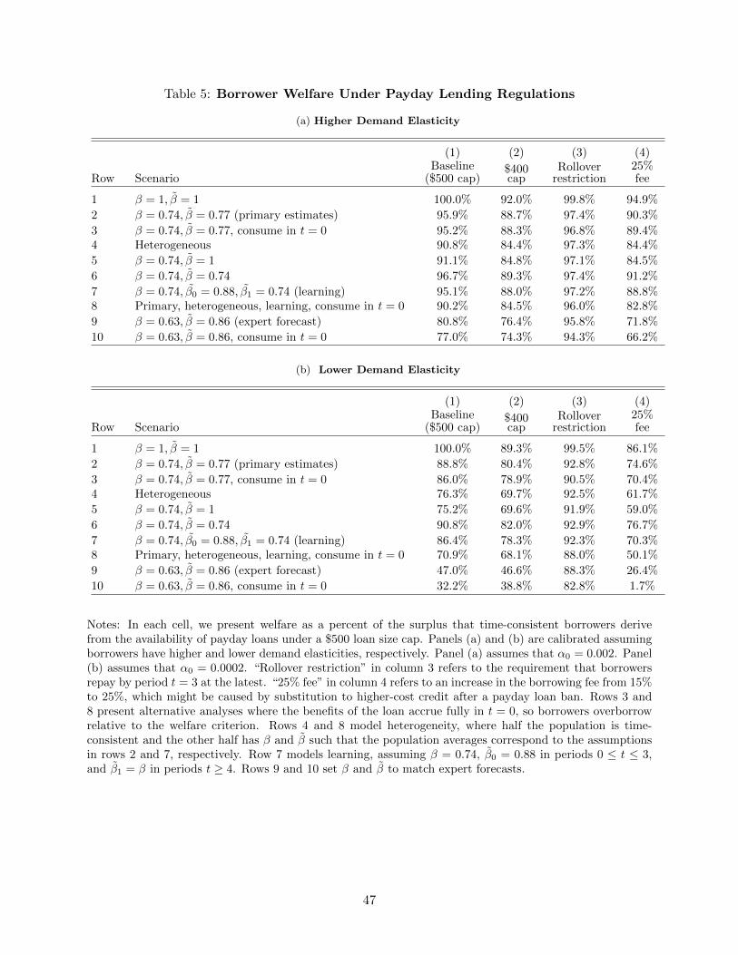
that under a standard $500 loan size cap, borrowers with our estimated β and β enjoy 89 to

96 percent as much surplus as a time-consistent borrower. Because borrowers are close to fully

sophisticated about repayment costs, payday loan bans and tighter loan size caps reduce welfare in

1In Section 5.1, we show that people overestimate the incentive’s effect on borrowing. This does not matter forour test: it requires only that people truthfully report their subjective beliefs on average, not that their subjectivebeliefs are correct.

3

our simulations. Limits on repeat borrowing increase welfare in some (but not all) specifications,

by inducing faster repayment that is more consistent with long-run preferences. These conclusions

are robust to various assumptions about heterogeneity in present focus and naivete.

Before we released the paper, we surveyed academics and non-academics who are knowledgeable

about payday lending to elicit their policy views and predictions of our empirical results. We use

the 103 responses as a rough measure of “expert” opinion, with the caveat that other experts not

in our survey might have different views. Our results contrast sharply with the weight of expert

opinion in our survey. Our average expert believed that borrowers would be much more naive

than they actually are—specifically, that borrowers would underestimate their future borrowing

probability by 30 percentage points, in contrast to the actual 4 percentage points. Furthermore,

more than half of our experts believed that payday loan bans are good for borrowers, and repeat

borrowing limits were slightly less popular than bans. In contrast, our model suggests that repeat

borrowing limits could benefit consumers, while bans do not.2

We highlight five important caveats. First, our parameter estimates are local to the 1,205

people in our experiment, although our sample does not differ substantially on observables from

typical payday borrowers. Second, our welfare analyses take the long-run preferences of present-

focused borrowers as being normatively relevant; this “long-run criterion” is common but somewhat

controversial (Bernheim and Rangel 2009; Bernheim 2016; Bernheim and Taubinsky 2018). Using

a different welfare criterion would likely strengthen our model’s prediction that most regulation

reduces welfare. Third, we model borrowing and repayment choices for an exogenous set of potential

borrowing spells with exogenous initial liquidity demand, instead of modeling individuals who

choose when to borrow over their lifetimes. As a result, we do not capture the possibility that

rollover restrictions might result in more (albeit shorter) spells, or that people might keep larger

buffer stocks in response to payday borrowing restrictions. However, additional analyses provide no

empirical support for those hypotheses: people do not keep significantly more liquid assets in states

with payday loan bans or in years after their state imposes a ban. Fourth, our analyses assume that

there are no market failures or behavioral biases other than present focus and misprediction. Fifth,

our results about the welfare benefits of payday lending consider markets with existing regulations

such as moderate loan size caps and truth-in-lending requirements, and thus do not speak to the

effects of deregulation.

Section 1 discusses related literature. Sections 2–5 present the background, experimental design,

data, and reduced-form empirical results. Section 6 presents the present focus model and estimation,

Section 7 presents our behavioral welfare evaluation of payday lending regulations, and Section 8

concludes.

2These prescriptions are consistent with arguments by Skiba (2012) and Morse (2016).

4

1 Related Literature

Our work builds on several existing literatures. One literature uses quasi-experimental variation to

evaluate the impacts of payday loan access (Zinman 2010; Melzer 2011, 2018; Morse 2011; Morgan,

Strain, and Seblani 2012; Carrell and Zinman 2014; Bhutta, Skiba, and Tobacman 2015; Bhutta,

Goldin, and Homonoff 2016; Carter and Skimmyhorn 2017; Gathergood, Guttman-Kenney, and

Hunt 2019; Skiba and Tobacman 2019). These papers consider a variety of different outcomes and

find a mix of positive and negative effects. Such impact evaluations can be difficult to use for welfare

analysis because it is not clear how to trade off effects on different outcomes, how to consider other

unmeasured welfare-relevant outcomes, or how to evaluate regulations such as rollover restrictions

that change the payday loan product instead of eliminating access. This highlights the need for

welfare analyses that include explicit measures of consumer bias. Our paper is the first to do this

for payday lending.3

We also build on existing papers studying imperfect information and behavioral biases among

payday loan borrowers. Bertrand and Morse (2011) show that providing information to first-time

borrowers about fees and the likelihood of repeat borrowing reduces borrowing. This result is

consistent with our finding of naivete among inexperienced borrowers, as the information could

induce sophistication and reduce borrowing.4 Mann (2013) asks borrowers how long they think it

will be before they go an entire pay period without borrowing, finding that 60 percent of borrowers

predict correctly within three days. However, Mann (2013) does not present formal statistical tests

of whether borrowers are biased on average, and his sample includes only people who have not

borrowed in the last 30 days, which may limit the generalizability of his results. Leary and Wang

(2016) show that one reason for payday borrowing is failure to plan for predictable income shocks.

Carter et al. (2019) find that payday borrowers who are quasi-experimentally granted more time

to repay loans do not repay more, and they show that this is consistent with a model of present

focus. Carvalho, Olafsson, and Silverman (2019) show that laboratory measures of decision quality

are negatively correlated with high-interest borrowing in Iceland. Relative to these papers, a key

contribution of our work is a theoretically driven design that allows us to estimate a model of

borrowing behavior, which then allows us to carry out a quantitative behavioral welfare analysis.

Skiba and Tobacman (2018) use observational data on payday borrowing to estimate a present

focus model. Their identification exploits the timing of default: in their model, naivete is required

to explain long borrowing spells ending in default, as sophisticates would default earlier to avoid the

interest payments. More recent work by Heidhues and Strack (2019), however, shows that the timing

of choices cannot be used to identify either β or β without additional parametric assumptions, as

3For other examples of this approach to behavioral policy evaluation, see Abaluck and Gruber (2011), Allcott andTaubinsky (2015), Allcott, Lockwood, and Taubinsky (2019), Bronnenberg et al. (2015), Chetty, Looney, and Kroft(2009), Grubb and Osborne (2015), Handel (2013), Handel and Kolstad (2015), Handel, Kolstad, and Spinnewijn(2019), Taubinsky and Rees-Jones (2018), and Rees-Jones and Taubinsky (Forthcoming); see Bernheim and Taubinsky(2018) for a review.

4Burke, Leary, and Wang (2016) show that this information provision had material effects when implementedthroughout Texas.

5

every distribution of stopping times can be rationalized by a time-consistent model with a different

distribution of unobserved shocks. For example, with a right-skewed distribution of income shocks,

one might reborrow repeatedly in hopes of repaying upon a high income draw and then default if

that high draw doesn’t come.5

Finally, our identification strategy for β and β advances the large empirical literature on present

focus. Many lab and field experiments document preference reversals, demand for commitment,

overoptimism, or other evidence of naive or sophisticated present focus without estimating model

parameters.6 Another set of experiments and field studies estimate part of a present focus model,

for example identifying β while assuming that people are fully naive or fully sophisticated.7 There

are only a handful of papers that estimate a full model of partially naive present focus.8 Our iden-

tification strategy is closest to that of parallel work by Carrera et al. (2019), which we extend and

generalize substantially to applications that involve non-separable dynamic programming models

with diminishing marginal utility from money and income effects.

2 Payday Lending Background

Payday loans are small, high-interest, single-payment consumer loans that typically come due on

the borrower’s next pay date. In the Lender’s data, typical loan maturities are about 14 days for

people on weekly, biweekly, or semimonthly pay cycles, and about 30 days for people on monthly

pay cycles. In 2016, Americans borrowed $35 billion from storefront and online payday lenders,

paying $6 billion in interest and fees (Wilson and Wolkowitz 2017). In Indiana, the site of our

experiment, lenders disbursed 1.2 million payday loans for a total of $430 million in 2017 (Evans

2019).

Indiana law caps loan sizes at $605 and caps the marginal interest and fees at 15 percent of

the loan amount for loans up to $250, 13 percent on the incremental amount borrowed from $251-

$400, and 10 percent on the incremental amount borrowed above $400. The Lender and its main

competitors charge those maximum allowed amounts on all loans. The annual percentage rate

(APR) for a 14-day loan with 15 percent interest is 391 percent, meaning that borrowing $100 over

each of the approximately 26.1 two-week periods in a year would incur $391 in interest. Regulations

vary across states (NCSL 2019), although Indiana’s price and loan size caps are close to the norm.

5The extent to which this matters is unclear: Martinez, Meier, and Sprenger (2020) show that present focusparameter estimates are not very sensitive to distributional assumptions in their tax filing application, while Heidhuesand Strack (2019) provide calibrated examples where parameter estimates are highly sensitive.

6See, for example, Ashraf, Karlan, and Yin (2006), Beshears et al. (2015), DellaVigna and Malmendier (2006),Duflo, Kremer, and Robinson (2011), Goda et al. (2015), Gine, Karlan, and Zinman (2010), John (forthcoming),Kaur, Kremer, and Mullainathan (2015), Kuchler and Pagel (2018), Read and van Leeuwen (1998), Royer, Stehr,and Sydnor (2015), Sadoff, Samek, and Sprenger (forthcoming), Schilbach (2019), Shapiro (2005), and Toussaert(2018).

7See, for example, Acland and Levy (2012), Andreoni and Sprenger (2012a; 2012b), Augenblick (2018), Augenblick,Niederle, and Sprenger (2015), Fang and Silverman (2004), Laibson et al. (2015), Mahajan, Michel, and Tarozzi (2020),Paserman (2008), and Shui and Ausubel (2005). See Imai, Rutter, and Camerer (2020) for a meta-analysis of presentfocus estimates from the Andreoni and Sprenger (2012a) convex time budget approach.

8To our knowledge, these are Augenblick and Rabin (2019), Bai et al. (2018), Carrera et al. (2019), Chaloupka,Levy, and White (2019), and Skiba and Tobacman (2018).

6

To take out a payday loan, borrowers must present identification, proof of income (e.g. a

paycheck stub or direct deposit slip), and a post-dated check for the amount of the loan plus

interest. Payday lenders do minimal underwriting, sometimes checking data from a subprime

credit bureau. By law, payday lenders in Indiana must report all loans to a database managed

by a company called Veritec. Lenders must check that database before disbursing loans to ensure

that people do not borrow from more than two lenders at once. We ran our experiment in Indiana

because we received regulatory approval to match consenting survey participants to their borrowing

records from this database.

When the loan comes due, borrowers can repay (either in person or by allowing the lender to

successfully cash the check) or default. After borrowers repay the principal and interest owed on

a loan, they can immediately get another loan. In some states, loans can be “rolled over” without

paying the full amount due, but Indiana law does not allow this. Per Indiana law, a borrower can

get up to five consecutive loans from a given lender. After that, the borrower cannot take out a

new loan from any lender for seven days. This rollover restriction has limited impact because it

lasts less than one pay cycle, so people can get another loan before they get close to running out

of money before their next paycheck arrives.

In 2017, 80 percent of the Lender’s loans nationwide were followed by another loan within the

next eight weeks. In principle, people can borrow any continuous amount. In practice, most people

make a binary decision to either reborrow the same amount or not get a new loan. Appendix Figure

A1 shows that of all consecutive loans disbursed nationwide by the Lender in 2017, 68 percent of

the subsequent loans were for the exact same amount as the previous loan, while 17 percent were

for more and 15 percent were for less. We will use this fact to simplify our model.9

If the borrower does not come to the store to repay the loan, the lender attempts to cash the

post-dated check, and is allowed by state law to do so up to three times. For bounced checks, the

borrower’s bank will likely charge a fee of about $30, and lenders in Indiana charge an additional

$25 bounced check fee. State law does not permit late fees. If the loan remains unpaid, the Lender’s

local staff try to work out a repayment plan with the borrower. If that fails, the Lender occasionally

refers an account to a third-party collection agency. The Lender does not lend to people who have

unpaid balances from past loan cycles.

Default is relatively rare on a per-loan basis: in 2017, only 3 percent of the Lender’s loans ended

in default. However, about 16 percent of loan sequences ended in default in that year.

Payday lending has the hallmarks of a competitive market. Entry requires only modest physical

capital, technology, and regulatory compliance relative to many other industries. There are about

300 payday lending stores in Indiana, of which the majority are owned by three national chains

(Evans 2019). Despite high interest rates, risk-adjusted profits appear to be low: Ernst & Young

(2009) estimated pre-tax profit margins of less than 9 percent on the borrowing fees, with the

majority of the costs due to operating costs (62 percent) and defaulted loans (25 percent). Thus,

9This fact is notable because depending on the distribution of income shocks, a standard model might predictthat borrowers would gradually pay down the principal instead of repeatedly borrowing the same amount and thenrepaying in full.

7

market power is unlikely to be an economically meaningful distortion in this industry.

Substitutes for storefront payday loans include online loans, checking account overdrafts, auto

title loans, pawn shops, loans from friends and family, and paying bills late. There is some disagree-

ment across datasets about how much liquidity payday borrowers might have available on credit

cards, which have much lower interest rates (Agarwal, Skiba, and Tobacman 2009; Bhutta, Skiba,

and Tobacman 2015).

The Lender and its main competitors transparently disclose the interest and other fees, in both

absolute levels and APRs, both in stores and on their websites. Furthermore, the CFPB’s 2017

regulation would limit the number of times that lenders can attempt to cash borrowers’ checks,

which generates the main fees that could be less salient to borrowers. For this reason, we do not

study shrouded fees as a motivation for additional regulation.

3 Experimental Design

We designed the experiment to answer two key questions: whether people anticipate repeat borrow-

ing, and whether people are willing to pay a premium for an incentive to avoid future borrowing.

The experiment ran at 41 of the Lender’s stores in Indiana from January 7th through March

29th, 2019, for two weeks in each store. We piloted and refined the survey extensively in fall 2018,

including follow-up interviews with store staff and with people who had taken the survey to check

their interpretation and understanding of the questions.

We contracted with a research company called EA Consultants to place a recruiter in each

center on most days. The recruiter would approach customers either before or after they took

out a loan and ask them to take a survey on an iPad. The iPad survey was self-contained, so

the recruiters were only needed to recruit and answer questions if they arose. Perhaps as a result

of the extensive piloting and refinement, the recruiters reported that they received essentially no

questions about the survey.

Survey details. Appendix I presents the full survey instrument. To be eligible, a person must

have taken out a payday loan from the Lender in Indiana in the past 30 days. After securing

informed consent, the survey asked people’s name and date of birth (to match to borrowing records)

and email address (to send gift cards as payment for participation).

The first substantive question on the survey was to ask people to report the probability that

they would take out another payday loan from any payday lender in the next 8 weeks. The possible

answers were 0%, 10%, 20%, ..., 90%, 100%.

The survey then introduced the first reward for completing the survey, “$100 If You Are Debt-

Free.” Participants were told that if they were selected for this reward, we would send them a

Visa cash card 12 weeks from now if they did not take out another payday loan from any lender

in the next eight weeks. The survey clarified that “All payday lenders are required to report loans

to a database. We will use that database to check your borrowing from all payday lenders.” We

8

included a comprehension check question to make sure that participants understood the incentive.

We then asked people to report the probability that they would take out another payday loan from

any payday lender in the next eight weeks, if they were offered $100 If You Are Debt Free; we call

this P in this section only.

Rewards and multiple price lists. After the belief elicitations were complete, the survey

introduced the second possible reward: a certain payment that we called “Money for Sure.” Just

as with the $100 If You Are Debt Free reward, Money for Sure would be paid within 12 weeks

on a Visa cash card. The survey then walked participants through an adaptive series of questions

to determine their valuations of the no-borrowing incentive. The first question asked whether the

person would prefer to receive the no-borrowing incentive or an amount of Money for Sure equal to

the incentive’s expected value. We helped people to calculate that expected value and highlighted

the non-financial reasons why they might prefer a certain payment versus a no-borrowing incentive.

The survey read,

Earlier, you told us that you have a [P ]% chance of getting another payday loan before

[8 weeks from now] if you are selected for $100 If You Are Debt-Free. In other words,

you would have a [100−P ]% chance of being debt-free. So on average, $100 If You Are

Debt-Free would earn you $[100− P ].

Given that, which reward would you prefer?

• $100 If You Are Debt-Free. This gives you extra motivation to stay debt-free.

• $[100− P ] For Sure. This gives you certainty and avoids pressure to stay debt-free.

The survey then sequentially offered choices with different amounts of Money For Sure in order to

bound the amount at which the borrower was indifferent between the certain payment and $100 If

You Are Debt-Free.10

The third possible reward for completing the survey was called Flip a Coin for $100. Participants

who were selected for this reward would have a 50 percent chance of winning $100 and a 50 percent

chance of winning nothing. This would also be paid within 12 weeks on a Visa cash card. The

survey led participants through an analogous adaptive question procedure, beginning with a tradeoff

between Flip a Coin for $100 and $50 For Sure. People’s valuations of Flip a Coin for $100 from

this procedure provide a measure of risk aversion.

10Because the survey allowed probabilities P to take values 0%, 10%, ..., 90%, 100%, the initial offer of Money ForSure could take values from $0, $10, ..., $90, $100. If the borrower preferred the no-borrowing incentive over 100−PFor Sure, the survey would offer another choice with 100−P + 20. If the borrower preferred 100−P + 20, the surveywould offer 100 − P + 40. If the borrower preferred 100 − P + 40, the survey would backtrack to 100 − P + 10 toavoid giving the mistaken impression that this was a bargaining game. Once the borrower preferred x For Sure overthe no-borrowing incentive, the survey would offer x− 10 for Sure. After that question, the borrower’s valuation ofincentive would be bounded within a $10 range. The algorithm worked analogously if the borrower initially preferred100− P For Sure over the no-borrowing incentive.

9

Attention check and qualitative questions. Immediately after this second MPL, there was

an attention check question in which the text asked people to click the “next” button instead of

answering. The survey ended with three qualitative questions designed to elicit intuitive measures

of desired motivation to avoid future borrowing and of past misprediction of payday borrowing.

Randomization and incentive compatibility. The computer used people’s responses on the

two adaptive procedures to fill out two multiple price lists (MPLs) with amounts of Money for Sure

ranging from $0 to $160 in increments of $10. Although all participants completed the MPLs, only

two percent of survey respondents (the “MPL group”) were ex-post randomly assigned to receive

the choice they made (or would have made) on a randomly selected row from one of the two MPLs.

Because all participants had a chance of having their MPL decisions determine their outcomes, it

was incentive compatible for participants to answer all questions truthfully. We informed people of

this before beginning the questions, saying “Think carefully, because the computer may randomly

select one of the following questions and give you what you chose in that question.” People could

click to a separate page for full implementation details.

We did not incentivize belief elicitations because truthful reporting is not incentive compatible

for individuals who perceive themselves to be time inconsistent. A person who thinks that she

borrows too much should report a borrowing probability that is lower than her actual belief, to

incentivize her future self to borrow less.11

The randomization assigned participants to $100 If You Are Debt-Free (the “Incentive group”),

no reward (the “Control group”), or the MPL group with 44, 54, and 2 percent probability, re-

spectively. Participants were randomized if they had “valid” survey data under four pre-registered

criteria: (i) if they passed both the no-borrowing incentive comprehension check and the attention

check, (ii) did not make inconsistent choices on either of the two MPLs, and (iii,iv) had certainty

equivalents of less than $160 on both of the two MPLs.

Post-survey. After the survey was complete, the iPad informed participants of whether they had

been selected for a reward. Each day, we matched surveys to the Lender’s records. Participants

whose name and birth date could be matched to a payday loan disbursed by the Lender in the

past 30 days were sent an email thanking them for participating and a reminder of any reward

that they had received. They also received a separate email from our gift card vendor explaining

how to claim their $10 gift card. People who began the survey but failed to complete received an

email encouraging them to complete their survey from where they had left off. People who took

out payday loans from a store on a day when the survey was available in that store were emailed

a link to take the survey online.

After four weeks, all participants received a second email, including a reminder of any reward

that they had received. After eight weeks, we received borrowing records from the Veritec statewide

database. By no more than 12 weeks after the survey (in practice, typically at 10 weeks), people

11Although Augenblick and Rabin (2019) show that this distortion is bounded in deterministic, continuous-effortsettings, this does not generalize to our stochastic discrete choice setting.

10

who had received Money For Sure or had been offered $100 If You Are Debt-Free and had not

borrowed were sent an email from our gift card vendor explaining how to claim their cash cards.

4 Data

4.1 Survey and Borrowing Data

13,191 people took out payday loans from one of the Lender’s stores on a day when the survey was

available in that store. We have the Lender’s records for those 13,191 loans, plus all loans from 2012

through February 2018 for a random sample of the Lender’s customers nationwide who took out

payday loans either online or in storefronts. The Lender’s data include income, an internal credit

score on a scale from 0–1000, pay cycle length, loan length, and loan amount. For our analyses

using the Lender’s nationwide data, we use all loans disbursed in 2017, the most recent complete

year. From the statewide payday lending database managed by Veritec, we also observe whether

each survey participant got another loan from any lender over the next eight weeks after they

took the survey. Payday borrowers typically borrow from only one lender, and reborrowing rates

are almost exactly the same whether calculated with the Lender’s data or with the Veritec data.

Appendix Table A1 presents more information on our key variables and their sources. Appendix

Table A2 documents that the Incentive and Control groups are balanced on observables.

Of the 13,191 people who took out loans on survey days in survey stores, 2,236 consented and

2,122 completed the survey, of whom 1,205 had valid survey data under the four pre-registered

criteria introduced in Section 3. See Appendix Table A3 for details. Unless otherwise noted,

figures and tables in the paper are limited to the 1,205 borrowers with valid data, following our

pre-registered sample inclusion criteria.12 Three percent of surveys were completed by borrowers

who had not responded in the store and were invited by email. Although our valid sample comprises

only a small share of customers who could have taken the survey, Table 1 shows that they are

comparable on our observable characteristics to the 13,191 borrowers on survey days and to the

Lender’s borrowers nationwide in 2017. The average loan length in our survey sample is 16 days,

the average loan amount is $373, and borrowers’ average annual income is about $34,000.

To cleanly compare predicted and actual borrowing, our survey participants’ borrowing after

the survey must not be affected by unexpected common shocks. For example, if unemployment

suddenly rose in the two months after the survey, this could cause an unpredicted borrowing increase

that our framework would attribute to naivete. Appendix Figure A4 shows that in Indiana over

the study period, per-capita income growth was steady and unemployment varied by only 0.1

percentage points.

We say that borrowers reborrowed if they were issued another loan from any payday lender at

any point between the day they took the survey and eight weeks after the survey. We say that

borrowers defaulted on a loan if they did not pay off all principal and fees owed. We say that

borrowers repaid if they did not reborrow or default—that is, if they did not owe debt to a payday

12The pre-registration is available at www.socialscienceregistry.org/docs/analysisplan/2037.

11

lender at any point between the day their current loan (at the time of the survey) came due and

eight weeks after the survey. We define a loan sequence (or borrowing spell) as a series of loans

with no more than eight weeks between any two loan disbursals.

4.2 Expert Survey

Before releasing our paper, we elicited predictions of our results and opinions about payday lending

regulation from a sample of domain experts, following recent work by DellaVigna and Pope (2018)

and others. We surveyed both academic and non-academic experts. For academics, our sample

frame was behavioral and household finance economists we cited in our April 2019 draft, plus

participants before two seminar presentations in April 2019. For non-academic experts, the sample

frame was (i) the chief consumer finance regulator in each of the 50 states plus DC, (ii) the lead

staff person for each Congressperson and Senator on the federal House and Senate financial services

committees, (iii) researchers and regulators working on consumer lending and credit from the CFPB

and the Department of Defense, and (iv) leadership and head payday lending experts at five major

think tanks (the Pew Center, the Center for Financial Services Innovation, the Consumer Federation

of America, the National Consumer Law Foundation, and the Center for Responsible Lending).

The survey began with a detailed description of our study’s context and sample, followed by

two sets of questions. First, we elicited opinions about whether three common types of payday

lending regulation were good or bad for consumers, and the certainty that the expert had in her

answer. Second, we elicited predictions of our empirical results. To elicit expert beliefs about

borrowers’ misprediction, we asked if the experts thought that the average payday loan borrower

underestimates, overestimates, or correctly foresees the chance that she will reborrow in the future.

We then told experts that borrowers in our data had about a 70 percent chance of reborrowing

over the next eight weeks, and asked for their estimate of borrowers’ average predicted reborrowing

probability.13 To elicit expert beliefs about borrowers’ demand for behavior change, we asked

if the experts thought that “the average payday loan borrower would want to give herself extra

motivation to avoid re-borrowing.” For experts who reported that they had a PhD in economics,

we also elicited their estimate of borrowers’ average β parameter.

We had 103 respondents, of whom 68 percent work at a university and have a PhD in economics.

See Appendix Table A4 for descriptive statistics. Appendix J presents the full expert survey

instrument.

5 Reduced-Form Empirical Results

This section presents answers to our two empirical research questions using only minimal modeling

assumptions.

13We said 70 percent because we did not yet know the sample average reborrowing probability when we fielded theexpert survey.

12

Define b as possible amounts of a no-borrowing incentive and γ = $100 as the actual incen-

tive offered in our experiment. Define µ(b) and µ(b) as the actual and perceived probabilities of

reborrowing over the next eight weeks. Define w(b) as a borrower’s valuation of a no-borrowing

incentive of amount b, i.e. the w(b) such that the borrower would be indifferent between a b dollar

no-borrowing incentive and w(b) dollars of Money for Sure. To be concise, we often use w (with no

argument) to refer to the w(γ) elicited on the survey.

Figure 1 illustrates the framework guiding our analysis. The x-axis is the probability of borrow-

ing in the next eight weeks, and the y-axis is the cost of borrowing. There are three demand curves:

actual, predicted, and desired. In a standard model of time-consistent consumers with rational ex-

pectations, these three curves coincide. Actual and predicted demand differ if people mispredict

future borrowing due to naivete about self-control problems, overoptimism about or inattention to

future income or expenditure needs, or any other reason. Predicted and desired demand differ if

people perceive themselves to be time inconsistent.

5.1 Do Borrowers Anticipate Repeat Borrowing?

We begin by comparing predicted and actual borrowing in the standard environment without the

experimental no-borrowing incentive. Figure 2 shows that the average borrower predicts she has a

µ(0) ≈ 70 percent chance of borrowing without the incentive, while in reality, µ(0) ≈ 74 percent

of borrowers in the Control group did borrow. This implies that the average borrower almost fully

anticipates repeat borrowing.14 Although our pre-registered exclusion restrictions could in principle

be correlated with sophistication, we find that is not the case: Appendix Figure A10 shows that

the results are largely the same when we do not apply the restrictions.

This slightly underestimated borrowing probability is consistent with responses to an additional

qualitative survey question. When asked how their past expectations of payday loan usage had lined

up with reality, 36, 25, and 39 percent of borrowers reported getting payday loans “more often than

I expected,” “less often than I expected,” and “about as often as I expected,” respectively. This

response distribution is close to the rational expectations benchmark, under which equal shares of

people would report borrowing “more often” and “less often” than expected.

Figure 3 presents misprediction as a function of recent borrowing experience. The four expe-

rience groups are approximately quartiles of the experience distribution in our sample. Borrowers

who had gotten three or fewer loans in the previous six months underestimate future borrowing by

20 percentage points, whereas borrowers with four or more recent loans predict close to correctly on

average.15 This is consistent with borrowers learning from experience—either about their present

14The samples in the left and right spikes of Figure 2 are different in that the left spike includes the full sample whilethe right spike includes the (randomly assigned) Control group only. This makes little difference for the conclusionbecause there is only minimal sampling error: the Control group’s predicted borrowing probability without theno-borrowing incentive is 69 percent.

15Over-optimistic beliefs are sometimes attributed to aspirational reporting, where time-inconsistent people misre-port beliefs in order to encourage future behavior change (Augenblick and Rabin, 2019). The fact that experiencedborrowers are on average exactly right suggests that this and related reporting biases did not affect their reports,although such factors could in principle affect less experienced borrowers.

13

focus or about the consequences of borrowing, as we discuss further in Section 6.8. It is also possible

that this correlation is due to unobserved factors that positively correlate with both reborrowing

and sophistication, although it is unclear what these factors might be, and our model in Section 7

predicts a negative correlation: all else equal, sophisticated types reborrow less, which would imply

a learning effect even larger than suggested by the correlation in Figure 3.16

This evidence that experienced borrowers are sophisticated differs from evidence of substantial

naivete in other settings. One potential explanation is that learning is context-specific, and payday

borrowing is a high-stakes domain with clear feedback and repeated learning opportunities.17

Appendix B further explores borrowers’ beliefs, showing that predicted and actual borrowing

are positively correlated. This relationship is attenuated relative to a 45-degree line because of

survey response noise due to rounding and other cognitive difficulties in articulating probabilities.

However, we show in the appendix that this does not bias our estimate of individuals’ average

forecast, because rounding leads to approximately mean-zero measurement error in people’s true

subjective beliefs.

The respondents to our expert survey believed that borrowers would be much more naive than

they actually are. 78 percent of our respondents thought that the average borrower underestimates

reborrowing. Figure 4 presents the distribution of respondents’ beliefs about borrowers’ average

predicted reborrowing probability. The average respondent thought that the average borrower

would predict only a 40 percent chance (standard error = 2.1 percent) of reborrowing over the next

eight weeks, a 30 percentage point misprediction relative to the 70 percent reborrowing probability

we told the experts. This contrasts sharply with the limited misprediction documented in Figure

2.

Misprediction in Incentive condition. A related but different question is whether people

correctly predict their borrowing in the Incentive condition. The average borrower predicts that

she has only a µ(γ) ≈ 50 percent chance of borrowing if offered the no-borrowing incentive, while

in reality, µ(γ) ≈ 70 percent of borrowers in the Incentive group did borrow. Putting this together

with the averages in Figure 2, this implies that the average borrower predicts that the no-borrowing

incentive would reduce borrowing by ∆ := µ(0)− µ(γ) ≈ 20 percentage points, whereas in reality,

the incentive reduced borrowing by only µ(0)− µ(γ) ≈ 3.8 percentage points.

There are several potential explanations. First, even if borrowers correctly predict their status

quo borrowing probability, they might overestimate their demand response if liquidity shocks have

16Appendix Figure A11 shows qualitatively similar results after defining experience to be the number of previousloans in the current loan cycle. Appendix Figure A12 shows that the decrease in misprediction with experience isdriven mostly by higher predicted borrowing probability, not lower actual borrowing probability. Appendix FigureA13 shows that misprediction does not differ statistically by internal credit score or income.

17Settings where significant naivete has been documented include real-effort laboratory experiments (Augenblickand Rabin 2019), which are low-stakes one-shot settings, and gym attendance (DellaVigna and Malmendier 2004;Acland and Levy 2015; Carrera et al. 2019), which has repeated learning opportunities but relatively low stakes.Kaur, Kremer, and Mullainathan (2015) and Yaouanq and Schwardmann (2019) find that people become moresophisticated over time in experiments with clear and salient feedback. Theoretical models show that learning isenhanced by stakes in the presence of partial commitment devices (Ali 2011), or by the possibility of many futurecontracting opportunities (Gagnon-Bartsch, Rabin, and Schwartzstein 2019).

14

higher variance than they realize. Indeed, because of the lack of price variation in the payday

loan market, borrowers have little opportunity to learn their price elasticity. Second, because the

experimental incentive is new and unfamiliar, borrowers may have forgotten about it and failed to

predict that they would forget. Indeed, although our participants are liquidity constrained and we

sent two reminder emails, our gift card vendor reports that only 44 percent of the $100 gift cards

were claimed, compared with 76 percent of the $10 gift cards given as participation payments the

day after the survey. Third, experimenter demand effects could have caused people to overstate

their beliefs about the effect of the incentive.

Appendix Figure A14 shows that there is no relationship between experience and mispredic-

tion in the Incentive condition. Because experienced borrowers are more accurate in the Control

condition, this means that experienced borrowers are actually worse at predicting the effect of the

incentive relative to Control. This suggests that learning is context-specific and bias-specific. Bor-

rowers may be fairly sophisticated about their present focus in normal conditions, but very naive

about their propensity to forget in unfamiliar conditions.

Figure 5 presents estimates of the average predicted and actual effects of the incentive separately

for people who reported that the incentive would reduce their borrowing and people who reported

that it would not. Because of noise in reported beliefs, the latter group includes the five percent

of respondents who reported µ(γ) > µ(0), and splitting on reported beliefs may not be the same

as splitting on actual beliefs. The figure shows that the low predicted response group correctly

predicts that the incentive will not affect their borrowing and the high predicted response group

correctly predicts that the incentive will reduce their borrowing, but the latter group substantially

overestimates the actual effect.

The bulk of the evidence suggests that misprediction in the Incentive condition lacks external

validity: it appears to be driven by the unusual nature of the experimental incentive. Thus, we

use only the misprediction in the status quo Control condition to identify naivete. Our estimates

in Sections 5.2 and 6 rely only on the assumption that people truthfully reported their subjective

beliefs (on average) about the effect of the incentive on borrowing; the fact that these subjective

beliefs are incorrect does not matter. We explore robustness to this assumption in Section 6.

5.2 Do Borrowers Perceive Themselves to Be Time Consistent?

To identify perceived time inconsistency, we compare valuations of the no-borrowing incentive to

the valuation a time-consistent borrower would have. Our strategy exploits the fundamental link

between time consistency and the Envelope Theorem for dynamic optimization. A time-consistent

person’s expected utility is unaffected by marginal changes in her future behavior, since her future

behavior maximizes her current utility function (by definition). Thus, a time-consistent borrower’s

valuation of a marginal no-borrowing incentive equals the mechanical effect of the incentive on

cash-on-hand; the induced marginal behavior change has no effect. By contrast, future behavior

changes do have first-order effects on the expected utility of time-inconsistent people because they

do not share the preferences of their future selves. Thus, a time-inconsistent borrower’s valuation

15

of the no-borrowing incentive will include this additional effect.

Combining valuations of future price changes with predictions of future behavior thus allows

tests of whether people perceive themselves to be time inconsistent. To be clear, this is a test of

perceived, not actual, time inconsistency, and the test is robust to misprediction of the effects of

the no-borrowing incentive.

For intuition, examine Figure 1. For this figure, we assume that borrowers have constant

marginal utility from the experimental payments. The no-borrowing incentive of γ = $100 is

equivalent to giving people $100 while also increasing the price of borrowing by $100. Thus, a

time-consistent borrower values the incentive at $100 minus the consumer surplus loss from a $100

price increase. On the figure, this consumer surplus loss is area ABCD. Thus, borrowers who

perceive themselves to be time consistent will value the incentive at $100−ABCD.

However, borrowers who perceive themselves to be time-inconsistent predict that they will have

different preferences in the future than they do when they take the survey. The figure captures

this by distinguishing between predicted and desired demand. As drawn, desired demand is shifted

inward, meaning that borrowers want their future selves to borrow less. The perceived additional

utility gain from a marginal behavior change is the vertical distance between perceived and desired

demand, which integrates to the trapezoid ABEF over the behavior change induced by the γ = $100

incentive. Thus, borrowers who perceive themselves to be time inconsistent will value the incentive

at $100−ABCD +ABEF .

In Appendix D.1, we formalize this idea using the the general Envelope Theorem results de-

veloped by Milgrom and Segal (2002) for arbitrary choice-sets, which encompass almost any time-

consistent stochastic dynamic programming model. We summarize the key results here using sim-

plified notation.

Consider a time-consistent borrower determining her change in valuation w′(b)db from a marginal

incentive change db. Let m1 and m0, respectively, denote the expected marginal utilities of money

(for the time when the experimental payments are made) across states of the world in which the

person does and does not borrow. The borrower predicts that she will avoid borrowing with prob-

ability 1 − µ, and the expected marginal utility in that state of the world is m0, so the Envelope

Theorem implies that utility from the change db is (1 − µ)dbm0. Similarly, the expected utility

from w′(b)db Money for Sure is (µm1 + (1− µ)m0)w′(b)db.

Thus, the valuation w′(b)db of a marginal incentive change db satisfies

(µm1 + (1− µ)m0)w′(b)db︸︷︷︸expected utility from Money for Sure

= (1− µ)dbm0︸︷︷︸expected utility from incentive

. (1)

If the borrower is risk neutral over income, then m0 = m1, and w′(b)db = (1− µ)db. In practice,

we expect m0 ≤ m1, both because the income from a non-marginal incentive reduces marginal

utility and because people have higher marginal utility of income in the states of the world where

they need to borrow. This implies

w′(b)db ≤ (1− µ)db. (2)

16

To determine a borrower’s valuation of the non-marginal no-borrowing incentive γ, we integrate

over Equation (2) as formalized in Appendix D.1. Assuming that µ is locally linear in the incentive

over this range, we show in Appendix D.2 that borrowers who perceive themselves to be time

consistent must have

w(γ) ≤ w∗ :=

(1− µ(0) +

∆

2

)γ, (3)

where ∆ := µ(0)− µ(γ).18 With constant marginal utility, this holds with equality, and the right-

hand side is the valuation we derived graphically on Figure 1: $100−ABCD. Because the bound

uses subjective expectations µ, it is valid for borrowers who mispredict borrowing for any reason,

including if they unexpectedly forget about the no-borrowing incentive.

Now consider borrowers who perceive themselves to be time inconsistent. The standard En-

velope Theorem logic does not apply: borrowers who perceive themselves to be time inconsistent

believe that their future behavior will not optimize current utility, so their valuation of the in-

centive includes the current utility benefits from behavior change. The perception that one will

“overborrow” (“underborrow”) in the future relative to current preferences will increase (decrease)

valuations of the no-borrowing incentive. Valuations w above the valuation bound w∗ from Equa-

tion (3) are consistent with perceived overborrowing.19 Valuations below that bound could be

consistent with perceived underborrowing or with m0 < m1. Thus, we have a one-sided test of time

inconsistency. In Section 6, we impose additional structure to tighten the bound and allow two-

sided tests. Even the one-sided test, however, is significantly more powerful in detecting perceived

time inconsistency than is the take-up of commitment contracts with no financial upside, since

demand for such contracts is easily eroded by the need for flexibility in an uncertain environment

(e.g., Heidhues and Koszegi, 2009; Laibson, 2015; Carrera et al., 2019).

Figure 6 presents the key moments that identify time inconsistency. The first spike shows

that the average borrower in our sample values the $100 no-borrowing incentive at $52. The

second spike is the valuation bound for time-consistent borrowers from the right-hand side of

Equation (3): w∗ =(

1− 70% + 70%−50%2

)× $100 ≈ $40 on average. Since the average valuation

exceeds the average valuation bound, we infer that the average borrower perceives herself to be

time inconsistent. We refer to the difference between these first two spikes, i.e. the average of

w − w∗, as the “behavior change premium.” This is $12 on average, or 30 percent more than the

average valuation bound.

The third spike on Figure 6 shows that the average borrower is willing to pay $42 for the $100

coin flip. This implies material risk aversion, with a risk premium of about $8 for a 50 percent

chance of receiving $100. Thus, the $12 behavior change premium could be a loose lower bound on

18The bound continues to hold if µ is concave in b, and increases only slightly under reasonable functional formswhen µ is convex. For example, if µ′(γ) = 1

4µ′(0), constituting an arguably high degree of curvature, Equation

(3) becomes w(γ) ≤ [(1− µ(0)) + 0.6(µ(γ)− µ(0))] γ under a quadratic approximation to µ. See Appendix D.2 fordetails.

19If people understate their true predicted borrowing probability µ(γ) on the survey, then the valuation bound wecalculate is higher than the “correct” valuation bound, which biases against detecting perceived time inconsistency.

17

borrowers’ actual valuation of the behavior change induced by the incentive.

This perceived time inconsistency is consistent with qualitative survey responses. Panel (a)

of Figure 7 shows that 54 percent of people report that they would “very much” like to give

themselves extra motivation to avoid future payday loan debt, 36 percent report “somewhat,” and

only 10 percent “not at all.” Panel (b) shows that although many people want motivation to avoid

payday loan debt, they tend to think that restrictions on repeat borrowing would be bad for them.

This is consistent with uncertainty about liquidity shocks creating a need for flexibility. Responses

to these two questions are correlated: people who want more motivation are more likely to think

that borrowing restrictions would be good for them.

Appendix Figure A2 presents the distribution of valuations of the no-borrowing incentive. Fig-

ure 8 shows that the behavior change premium is correlated with other survey responses in expected

ways. People who report that they want more motivation to avoid payday loan debt, that a rollover

restriction would be good for them, or that the incentive will reduce their probability of borrowing

have higher behavior change premia.

6 Partially-Naive Present Focus Model

6.1 Model

The previous section shows that misperceived borrowing and perceived time inconsistency are iden-

tified with minimal assumptions. In this section, we use similar identification ideas and additional

assumptions to estimate a structural model of borrowers’ time preferences and beliefs.

We assume that borrowers have quasi-hyperbolic preferences given by Ut = ut+β∑T

τ=t+1 δτ−tuτ ,

where ut is the period t utility flow. Following O’Donoghue and Rabin (2001), we allow people to

mispredict their preferences: in all periods t < τ , they predict that their period τ self will have

short-run discount factor β. We discuss other misprediction models in Section 6.7.

Our model builds on Heidhues and Koszegi (2010). We focus on three periods of a potentially

longer or infinite-horizon model. In period 0, the borrower gets a loan of amount l and then takes

our survey. The next eight weeks after the survey are period 1. At the beginning of period 1,

the borrower receives a smoothly distributed transitory shock θ. This shock captures expenses

(such as car repairs) and income shocks (such as being scheduled for fewer hours at work) that are

unpredictable as of period 0. In period 1, the borrower chooses to either repay or reborrow. If she

repays, she pays the principal and fee l + p(l) in period 1 and receives no-borrowing incentive b in

period 2. If she reborrows, she pays only the fee p(l) in period 1, owes l + p(l) in period 2, and

does not receive the no-borrowing incentive.

For notational convenience, we define repayment cost and continuation cost functions, with the

understanding that these functions correspond to reduced consumption and reduced continuation

values. The cost of paying amount x in period 1 is a smooth function k(x, θ) that is convex in x and

strictly increasing in θ. The expected reduction in period 2 continuation value caused by period 2

debt x is C(x). The x in C(x) can be negative for borrowers who are owed an incentive payment.

18

For simplicity, the exposition in this section assumes that the borrower has the same expectation

C of period 2 continuation costs in both periods 0 and 1. However, the proofs of this section’s results

in Appendix E allow for certain types of correlated shocks that reveal additional information about

C in period 1.

The assumption of a well-behaved continuation cost function C is far from innocuous when

β < 1, because C is the solution to a non-cooperative game played between the different selves

(Harris and Laibson 2001; Laibson et al. 2015). In Appendix F.1, we show existence, uniqueness,

and smoothness of C in the fully dynamic model presented in Section 7.

Three assumptions of this framework should be made explicit. First, people cannot get a loan

of any amount other than l in period 1. As shown in Appendix Figure A1, this is realistic because

most people either repay or reborrow the same amount as their previous loan. Second, borrowers

cannot default in period 1. This is a reasonable approximation because the probability of default on

any one loan is only 3 percent. The microfounded model in Appendix F.1 allows people to default

in period 2 or later, so the possibility of default can influence the period 2 continuation value C.

Third, borrowers have only one borrowing decision in period 1.

To quantify the different marginal utilities m1 and m0 from Section 5.2, we use a quadratic

approximation to C(x). Let α := C′′(0)

C′(0)be the coefficient of absolute risk aversion at x = 0, and

define ρ := α(l + p). Under a quadratic approximation, ρ approximates the percent difference in

marginal utilities when people reborrow versus repay: ρ ≈ C ′(l + p)/C ′(0)− 1.

6.2 Demand for Payday Loans

This formulation allows us to put structure on the desired, predicted, and actual demand curves

from Figure 1. Define θ∗B as the cutoff value of θ at which the period 1 benefits of reborrowing

equal the discounted period 2 costs:

k(l + p, θ∗B)− k(p, θ∗B)︸︷︷︸period 1 utility benefit of reborrowing

= Bδ(C(l + p)− C(−b)

)︸︷︷︸

period 2 continuation cost of reborrowing

. (4)

The actual, predicted, and desired cutoffs θ∗B are derived from setting B = β, B = β, and B = 1,

respectively. The borrower reborrows when θ > θ∗β. When taking the survey in period 0, the

borrower predicts that she will reborrow if θ > θ∗β. To maximize period 0 utility, the borrower

would reborrow if θ > θ∗1. Actual, predicted, and desired demands are thus the probability that θ

exceeds θ∗β, θ∗β, and θ∗1, respectively.

The constant marginal utility case from Section 5.2 corresponds to linear C. Under this as-

sumption, Equation (4) can be written as

k(l + p, θ∗B)− k(p, θ∗B)

BδC ′= l + p+ b. (5)

Now the period 1 benefits and period 2 costs of reborrowing are in units of period 2 dollars,

consistent with the y-axis of Figure 1. Each borrowing probability on the x-axis corresponds to

19

a unique θ∗B, and thus a unique numerator on the left-hand side of Equation (5). Since predicted

demand uses B = β instead of B = β in the denominator, predicted demand is shifted down from

actual demand by proportion β/β on Figure 1. Since desired demand uses B = 1, desired demand

is shifted down from predicted demand by proportion β.

6.3 Identifying Sophistication versus Naivete

In Section 5.1, we compared predicted and actual demand to identify misprediction in probability

units. We now identify the relationship between β and β by transforming misprediction into

marginal utility units.

Define γ† such that µ(γ†) = µ(0). In words, γ is the no-borrowing incentive at which predicted

demand with the incentive would equal actual demand without the incentive. Under a linear

approximation, the perceived demand slope is −∆γ (where ∆ := µ(0)−µ(γ), as before), the definition

of γ† becomes µ(0) + γ† −∆γ = µ(0), and thus

γ† =γ

−∆(µ(0)− µ(0)) . (6)

This shows how γ† transforms misprediction µ(0) − µ(0) into dollar units using the perceived

demand slope γ

−∆. In Figure 1, γ† is the vertical distance between points H and G, the predicted

and actual demand curves at probability µ(0). γ† > 0 implies that people overestimate future

borrowing, while γ† < 0 implies that people underestimate borrowing. From Section 5.1, we know

that γ† < 0 on average in the data.

We can also write γ† as a function of β and β using the right-hand side of Equation (4). For

γ† to equate predicted demand at incentive γ† with actual demand at zero incentive, it must also

equate the predicted period 2 reborrowing cost at incentive γ† with the actual reborrowing cost at

zero incentive:

β[C (l + p)− C(0)

]︸︷︷︸

period t self’s borrowing cost

= β[C (l + p)− C(−γ†)

]︸︷︷︸

predicted borrowing cost with incentive γ†

. (7)

We can re-write this as a function of α and ρ using a quadratic approximation to C.

Proposition 1. Assume that terms of order (l + p+ b)3C ′′′ and µ′′γ2 are negligible. Then

β (l + p)(

1 +ρ

2

)︸︷︷︸

period t self ’s borrowing cost

= β(l + p+ γ†

)(1 +

ρ

2− α

2γ†)

︸︷︷︸predicted borrowing cost with incentive γ†

, (8)

where γ† = γ

−∆(µ(0)− µ(0)).20

20The quadratic approximation to C is increasing in γ† for all γ† < 0. The quadratic function (l+ p+x)(1 + ρ/2−α/2x) can be factored as (l + p + x)(2/α + l + p − x)α/2, which has its vertex at 1/α. Thus, γ† uniquely identifiesβ/β.

20

If C is linear, then ρ = α = 0, and thus

β

β=l + p+ γ†

l + p. (9)

We can see this equation on Figure 1. Both the left-hand side and right-hand side reflect the

ratio of the height of H to the height of G, i.e. the ratio of predicted to actual marginal utility at

probability µ(0). We infer lower β/β (more naivete) when γ† is more negative (people more heavily

underestimate future borrowing).

In Appendix E.1, we show that Equation (9) provides a lower bound on β/β under general

assumptions allowing any convex C (not just a quadratic approximation) and arbitrarily correlated

shocks to k and C.

6.4 Identifying Perceived Present Focus

In Section 5.2, we identified perceived time inconsistency by testing for whether people value the

no-borrowing incentive more than they would if they perceived themselves to be time consistent.

We now identify perceived present focus parameter β by putting more structure on that intuition.

For this section, we need to consider how predicted reborrowing µ depends on both Money for

Sure w and on the no-borrowing incentive b, and thus we sometimes write µ(w, b) in the derivations.

When µ has one argument, we continue to mean µ(b).

From the perspective of the period 0 self, the change in expected utility from a marginal change

in b at w = 0 is

dV

db= δ

[(k(l + p, θ∗β)− k(p, θ∗

β))− δ

(C(l + p)− C(−b)

)]︸︷︷︸

utility loss from marginal borrowing probability increase

µ′b(0, b)︸︷︷︸∆ behavior

+δ (1− µ(0, b))C ′(−b)︸︷︷︸mechanical effect

(10)

The “mechanical effect” is the expected utility gain from the increased incentive, holding behavior

constant. From Equation (4), the period 0 self predicts that the period 1 self will set k(l+ p, θ∗β)−

k(p, θ∗β) = βδ

(C(l + p)− C(−b)

). Substituting this into (10) yields

dV

db= δ2

−(1− β)(

C(l + p)− C(−b))

︸︷︷︸perceived internality

µ′b(0, b)︸︷︷︸∆ behavior

+ (1− µ(0, b))C ′(−b)︸︷︷︸mechanical effect

. (11)

This follows the Envelope Theorem discussion from Section 5.2. Borrowers with β = 1 perceive

that period 1 behavior maximizes period 0 preferences, so the first term inside the brackets drops

out and dVdb is just the mechanical effect of the incentive.

Using similar logic, the period 0 self’s change in expected utility from a marginal change dw in

Money for Sure at b = 0 is

21

dV

dw= δ2

−(1− β)(

C(l + p− w)− C(−w))

︸︷︷︸perceived internality

µ′w(w, 0)︸︷︷︸∆ behavior

+ (1− µ(w, 0))C ′(−w) + µ(w, 0)C ′(l + p− w)︸︷︷︸mechanical effect

.(12)

To compute the non-marginal effects of w and b, we integrate over the marginal conditions above

and set them equal. To obtain simple approximations to these integrals in terms of observables, we

continue to assume that µ is locally linear and take a quadratic approximation to C.

Proposition 2. Assume that terms of order (l+p)3C ′′′/C ′ are negligible and that µ is locally linear

and separable in w and b. Then

(1− αw

2

)w ·

(1 + ρ

(µ(0) +

wρ

γ

∆

2

))︸︷︷︸

utility from w if time consistent

−(

1− β)(

1 +ρ

2

)(l + p)︸︷︷︸

perceived internality

wρ

γ∆︸︷︷︸

∆(w) behavior

(13)

=(

1− αγ

2

) γ ·

(1− µ(0) +

∆

2

)︸︷︷︸

utility from γ if time consistent

+(

1− β)(

1 +ρ

2

)(l + p+

γ

2

)︸︷︷︸


∆︸︷︷︸∆(γ) behavior

.

The left-hand side is the expected utility of w(γ) dollars of Money for Sure, and the right-hand

side is the expected utility of the γ no borrowing incentive.

If C is linear, then α = ρ = 0, and this simplifies to

w =

(1− µ(0) +

∆

2

)γ︸︷︷︸

utility from γ if time consistent

+(

1− β)(

l + p+γ

2

)︸︷︷︸


∆︸︷︷︸∆(γ)behavior︸︷︷︸

internality reduction benefit

. (14)

We can see this equation on Figure 1. As discussed in Section 5.2, risk-neutral people who perceive

they are time consistent value the no-borrowing incentive at(

1− µ(0) + ∆2

)γ. The additional

structure in this section allows us to map the behavior change premium trapezoid ABEF to an

estimate of β. The height of the trapezoid is the difference between the weights that the period 0 and

period 1 self put on the perceived period 2 continuation cost of reborrowing:(

1− β) (l + p+ γ

2

).

The width is the change in borrowing probability ∆ := µ(0) − µ(γ). We infer a lower β (more

perceived present focus) when w is more positive (people are willing to pay more for the incentive

to avoid future borrowing).

22

6.5 Identifying Curvature

Our formulas can accommodate any curvature parameter α. One approach is to use borrowers’

certainty equivalents of the Flip a Coin for $100 lottery: lower certainty equivalents imply more

curvature. In Appendix E.3, we show that this implies a sample average α ≈ 0.0064.

The benefit of this approach is that α is elicited from our population of payday borrowers.

Curvature estimates from other populations may not be relevant: the fact that payday borrowers

carry costly debt suggests that their marginal utility may be sensitive to small gains and losses.

However, α ≈ 0.0064 may be too large: under a quadratic approximation, α ≈ 0.0064 implies that

an extra $100 of debt increases utility from the marginal dollar by 64 percent, and thus borrowers

who have $400 more debt (approximately the average loan size) in period 2 have 256 percent higher

marginal utility. One potential confound is that since the $100 lottery is smaller than most loans,

certainty equivalents may be affected by small-stakes risk aversion that is behaviorally distinct

from utility function curvature (Rabin 2000). For comparison, our lottery α estimate is 3 to 30

times larger than other estimates using higher-stakes field decisions such as insurance choice and

labor supply in less liquidity-constrained populations.21 In our empirical estimation, we therefore

consider multiple curvature values between α = 0.0064 and α = 0.

6.6 Empirical Implementation

In theory, Equations (8) and (13) hold for each individual borrower, and individual survey responses

could imply individual-specific β and β. In practice, any survey responses are noisy, so we observe

µ, w, and risk aversion with measurement error. Furthermore, since Equations (8) and (13) involve

squaring some of these survey response variables, we have non-classical measurement error that

cannot be addressed by simply taking expectations.

To address this, we define groups of observations indexed by g and calculate group-level averages

of the empirical objects in Equations (8) and (13), including γ†g = γµg(0)−µg(γ) (µg(0)− µg(0)). For

our primary estimates, we use the five groups defined by quintiles of loan size l.

In Appendix E.4, we show how we can substitute the group average variables into Equations

(8) and (13), take expectations over observations, and re-arrange, giving the following estimating

equations:

(β

β

)=

∑i

(lg + pg + γ†g

)(1 +

ρg2 −

αg2 γ†g

)∑

i (lg + pg)(1 +

ρg2

) (15)

and

21Using insurance decisions, Cohen and Einav (2007) estimate α ≈ (0.00087, 0.0019), Handel (2013) estimatesα ≈ (0.00019, 0.000325), and Sydnor (2010) estimates α ≈ 0.002. Chetty (2006) estimates a constant relative riskaversion coefficient of 0.7 from labor supply elasticities, which translates to α ≈ 0.0007 if payday borrowers have$1000 monthly “uncommitted” (in the sense of Chetty and Szeidl, 2007) consumption. Using relatively small-stakesgambles, van Gaudecker, van Soest, and Wengstrom (2011) estimate α ≈ 0.03, and Holt and Laury (2002) estimateα ≈ 0.2.

23

ˆβ = 1−

∑i

wg ·

(1 + ρg

(µg(0) +

wgρgγ

∆g

2

)) (1− αgwg

2

)− γ ·

(1− µg(0) +

∆g

2

) (1− αgγ

2

)∑

i

(1 +

ρg2

)∆g

(lg + pg + γ

2

) (1− αgγ

2

)+ (lg + pg)

wgρgγ

(1− αgwg

2

) . (16)

If β/β and β are homogeneous across borrowers, Equations (15) and (16) deliver unbiased

estimates as long as survey response error is mean-zero, so the expectations of wg, µg, µg, and

γ†g equal the true group means. If β/β and β are heterogeneous, Appendix E.4 lays out a set of

assumptions under which Equations (15) and (16) are unbiased. One key assumption is that terms

of order E[(1− βi)2|g] are negligible. This is reasonable because if we think that no borrowers have

β > 1, not many borrowers can plausibly have βi 1 given that our empirical estimate is that

the average βi is not far from one. A second key assumption is that E[βi|g] does not vary across

g. This is reasonable if we think that perceived time inconsistency is unrelated to loan size. Other

papers that estimate present focus models (e.g. Laibson et al. 2015; Skiba and Tobacman 2018)

assume homogeneity or comparable orthogonality conditions, although Bai et al. (2018) estimate a

distribution of unobserved heterogeneity.

If β/β and β are homogeneous or βi/βi is orthogonal to βi (i.e., people who think they are more

versus less present focused misperceive their true present focus by the same proportion on average),

then the sample average β is simply

β =

(β

β

)· ˆβ. (17)

Appendix E.4 shows that this estimator is also unbiased if βi is orthogonal to a naivete statistic1−βi1−βi introduced by Augenblick and Rabin (2019), which reflects the degree to which people think

their present focus is closer to 1 than it actually is.

We estimate standard errors by bootstrapping.

6.7 Other Sources of Misprediction

This section has interpreted misprediction µ(0) − µ(0) through the lens of a present focus model.

However, misprediction could also be driven by overoptimism about future income or expenditure

needs, or inattention to changes in those variables (Browning and Tobacman 2015; Karlan et al.

2016; Gabaix 2017). Our estimates of β do not depend on the magnitude or source of misprediction,

but our estimates of β could be affected.

For example, consider a model in which borrowers perceive that period 1 repayment costs k will

be factor κ ≤ 1 as large as they actually are. Then the right-hand side of Equation (7) is multiplied

by 1/κ, and the right-hand side of Equation (15) delivers an estimate of κ ·β/β. Intuitively, naivete

about present focus causes a borrower to think that the period 1 self will give immediate costs β/β

less weight than she does in reality, which is mathematically isomorphic to believing that period 1

costs will be κ smaller than they are in reality (Browning and Tobacman 2015).

24

If κ 6= 1, we cannot estimate β with Equation (17). However, if we assume that κ ≤ 1 and

β/β ≤ 1—that is, that borrowers are not underoptimistic and do not perceive themselves to be

future focused—then we can bound β on

[(β

β

)· ˆβ,

ˆβ

]using the estimates from Equations (15) and

(16). The lower bound is from the assumption that κ = 1, so all of misprediction is driven by

naivete about present focus, while the upper bound is from the assumption that β/β = 1, so all of

misprediction is driven by other factors.

While Section 5 showed that borrowers overestimated the effect the incentive would have on

borrowing, this should not affect our parameter estimates. We do not use misprediction in the

Incentive condition to identify β/β, and our estimate of β and the above bounds on β are valid

as long as respondents correctly reported their beliefs on average on the survey. This would be

the case under either of two plausible microfoundations for misprediction of the incentive effect: if

κ < 1 and borrowers thus underestimate the variance in repayment cost shocks, or if they forget

about the incentive with some probability in period 1, but naively fail to foresee this in period 0.

6.8 Parameter Estimates

Table 2 presents our parameter estimates. Column 1 presents the estimated average β/β, which

can also be interpreted as κ in a model where borrowers perceive that future repayment costs will

be share κ as large as they actually are. Column 2 presents the estimated average β. Column 3

presents the implied estimate of average β. As discussed in Section 6.7, this is a lower bound on β

if κ < 1.

The first five rows present estimates using the full sample at different values of α. The estimates

of β/β, β, and β are monotonic in α over this range, so the estimates for α ≈ 0.0064 and α = 0

provide bounds. Our point estimates of borrowers’ average β/β range from 0.95 to 0.98, reflecting

the fact that the sample slightly underestimates borrowing on average. For each α, β/β is statisti-

cally distinguishable from one with slightly more than 95 percent confidence. Our point estimates

of borrowers’ average β range from 0.76 to 0.87, and the upper end of the confidence intervals never

exceeds 0.90. Assuming less risk aversion increases β because it increases the modeled valuation

that a time-consistent borrower would have for the (risky) incentive, thereby reducing the premium

attributed to perceived internality reduction. The point estimates of β range from 0.74 to 0.83.

The next two rows present estimates for the subsample of borrowers who had gotten three or

fewer loans from the Lender in the six months before taking the survey, for the bounding high and

low values of α. The two rows after that present estimates for the complementary subsample with

four or more loans of recent experience. Consistent with Figure 3, more experienced borrowers are

fully sophisticated, with estimated β/β ≈ 1.00, while less experienced borrowers have β/β between

0.79 and 0.89. The point estimates for β differ modestly. Under the plausible assumption that

β ≤ β for all borrowers, this implies that experienced borrowers are all sophisticated, although

there is more scope for significant heterogeneity among the inexperienced borrowers.

The implied lower bounds on β are statistically different for the two groups, especially for α = 0.

There are two possible explanations. First, it could be that the groups’ actual β parameters are the

25

same, and the reduced misprediction in the experienced group is from learning about the utility

cost of repayment, not learning about present focus. Second, the different estimates could be driven

by experiential learning in the sense of Laibson’s (2018) “model-free equilibrium”: borrowers with

particularly low β learn that borrowing is delivering low payoffs, and they thus avoid borrowing.

In this model, borrowers do not necessarily learn an exact model of their preferences, and their

perceived β does not necessarily change—the low-β types simply select out of borrowing.

As discussed in Section 6.6, we estimate population average parameters under certain orthog-

onality and homogeneity assumptions. The final rows of Table 2 present estimates where we

separately estimate the parameters by above- versus below-median experience (our most important

moderator) and take the subsample size-weighted average of the two estimates within each boot-

strap replication. The resulting parameter estimates are almost identical to the primary estimates

in the earlier rows. Thus, accounting for heterogeneity along this key dimension does not affect our

estimates of the sample average.

So far, we have assumed that people correctly reported their beliefs (on average) on the survey.

If people instead overstated their true beliefs ∆ about the effect of the incentive, our parameter

estimates can be interpreted as bounds. β would be an upper bound (i.e. people perceive more

present focus than we estimate), because if predicted behavior is less responsive to the incentive than

people report, their internality reduction per unit of behavior change is higher than we estimate.

Sophistication would be an upper bound (i.e. β/β will be smaller than we estimate), because if

predicted demand is less responsive than people report, a given amount of misprediction in the

Control condition implies a larger difference in predicted versus actual marginal utility.

To explore possible magnitudes, we estimate β/β and β with alternative equations where we

set ∆ to half its reported amount, keeping α = 0.0064. That is, we assume that people report that

the incentive will reduce their borrowing probability by twice as much as they actually believe.

Under this assumption, β drops substantially to 0.54, and β/β decreases to 0.95. Thus, to estimate

β, it is crucial to assume that people reported their beliefs without bias. However, the fact that

this alternative assumption delivers a low β that is out of line with estimates from other domains

provides additional support for the assumption that people did correctly report their beliefs.

The respondents to our expert survey believed that borrowers would have less demand for

behavior change than they actually did. Only 56 percent believed that the average borrower would

want motivation to avoid future borrowing. By contrast, Figure 7 documented that 90 percent

of borrowers reported qualitatively that they wanted extra motivation to avoid payday loan debt.

Quantitatively, Figure 9 shows that most respondents overestimated borrowers’ average β. The

average respondent predicted β ≈ 0.86 (standard error = 0.03), which is larger than the point

estimates in Table 2 except at α = 0.

26

7 Policy Evaluation

In this section, we study the welfare effects of three common payday lending regulations: a payday

lending ban (in practice, effectuated by a low interest rate cap that causes all lenders to exit),

a rollover restriction (in practice, effectuated by a required “cooling off period” that disallows

additional borrowing for 30 days after three consecutive loans), and a loan size cap. In Section

7.1, we set up the model. In Section 7.2, we give theoretical intuition for how different parameters

affect welfare. In Section 7.3, we turn to numerical simulations.

7.1 Model

We continue with the model as described in Section 6, except that we endogenize the initial loan

amount, explicitly model reborrowing over many periods, and allow default. We also re-number

the periods, so periods 0–2 from Section 6 could represent any three periods in this section.

People borrow amount l in period t = 0. In each subsequent period t ∈ 1, ..., T, with T

possibly infinite, borrowers receive transitory shock θt and correlated shock ηt and then have three

options. First, they can repay l + p(l). In this case, the game ends. Second, they can pay the

fee p(l) and reborrow the principal l. In this case, the game continues. Third, they can default,

incurring immediate cost χ. In this case, the game ends.

Let u(l, ν) denote the benefit of borrowing amount l, where ν is a shock. Analogous to Section

6, the utility cost of paying amount x in period t is k(x, θt, ηt). Define C(l) as the actual cost,

in expectation using the t = 0 information set, of repaying a loan of size l beginning in t = 1,

and let C(l) denote the t = 0 self’s perception of that cost. These continuation cost functions are

endogenously determined by repayment cost function k(x, θt, ηt) and equilibrium borrower behavior.

Theorem 1 in Appendix F.1 shows that under some regularity conditions on k and θt, ηt, there

exists a unique equilibrium for finite T , and a unique stationary equilibrium for T = ∞, with

smooth continuation cost functions C and C.22

For welfare analysis, we use the “long-run criterion,” taking the preferences of the t = −1 self

to be normatively relevant. This is common (e.g. O’Donoghue and Rabin 1999, 2006; Carroll

et al. 2009) but not uncontroversial (Bernheim and Rangel 2009; Bernheim 2016; Bernheim and

Taubinsky 2018). Any welfare criterion that places more weight on the later selves’ preferences to

borrow would likely strengthen our conclusion that most regulation reduces welfare.

For our primary analysis, we follow Heidhues and Koszegi (2010) in assuming that the loan af-

fects utility only after period t = 0, as might be the case for a car repair that the borrower can afford

only by taking out a loan. Thus, the borrower chooses l in t = 0 to maximize βδ[u(l, ν)− C(l)

],

and the welfare criterion is βδ2 [u(l, ν)− C(l)]. We also present alternative analyses in which the

benefits of the loan accrue fully in t = 0, so the borrower maximizes u(l, ν) − βδC(l), and the

welfare criterion is βδ [u(l, ν)− δC(l)]. The difference between these two cases is that in our alter-

22We are able to establish these results even though the Bellman operator on the continuation value functions isnot a contraction. When T =∞, there may also be non-stationary equilibria in environments with minimal variationin θ and η. We use stationarity as an equilibrium refinement.

27

native analysis, the borrower “overborrows” relative to the welfare criterion even when C(l) = C(l),

since the benefits are immediate while the repayment costs are delayed. To avoid the mechanical

implication that borrowers with lower β derive less welfare, we normalize both welfare criteria by

1/β.

Our analyses consider only consumer welfare, and we abstract away from the supply side of the

market by assuming that the interest rate is exogenous. This is realistic given that interest rates

in Indiana and other states equal the regulated cap.

7.2 Theoretical Results

7.2.1 Setup

We now present theoretical intuition for the welfare effects of payday borrowing under different

assumptions for borrower types and the amount of volatility in θ and η. For borrower types, we

consider different assumptions for β and β, and we allow borrowers to learn their type, having

perceived present focus β0 ≥ β in period t = 0 and β1 ∈ [β, β0] for t ≥ 1. In this sub-section, we

assume infinite horizon (T =∞), which allows us to consider stationary equilibria, and we assume

that the long-run discount factor is δ = 1, which is a close approximation given that pay cycles are

two weeks to one month long.

7.2.2 Repayment Behavior and Costs

The effect of β and β on repayment costs depends on the amount of volatility in repayment cost

shocks θ, η. Proposition 5 in Appendix F.4 shows that with high enough volatility, present focus

and naivete have zero effect on repayment costs: regardless of β and β, borrowers repay in “good”

states and reborrow in “bad” states. Proposition 6 in Appendix F.4 shows that in the limit case of

vanishing volatility in θ and η, persistently naive (β1 > β) borrowers perpetually reborrow because

they are over-optimistic about repaying in the next period, which entices them to reborrow in the

current period. This generates infinite repayment costs C. This result echoes O’Donoghue and

Rabin (1999, 2001), who show that naive agents can infinitely delay an unpleasant task (such as

repaying a loan) in a deterministic setting.23

However, the limit case in Proposition 6 leads to stark and counterfactual predictions. First,

because borrowers predict that their future selves will be approximately indifferent between rebor-

rowing and repaying, they will believe that even small temporary incentives to repay next period

will ensure repayment that period. However, our belief elicitations reject this. Second, with even

23In Appendix F.6, we establish a type of “purification theorem” showing that as repayment cost shock volatilityvanishes, behavior converges to a stationary mixed strategy equilibrium of a deterministic game. Our frameworkdiffers from O’Donoghue and Rabin (1999, 2001) in three main ways. First, because our borrowers choose theirloan amounts in t = 0, the welfare effects of present focus and naivete operate on that margin as well. Second, ourborrowers have the option to default. Third, we allow uncertainty in repayment costs, which substantially changesthe equilibrium and results. In a deterministic environment, O’Donoghue and Rabin show that sophisticated typesplay pure strategies with cycles, for example completing the task only in periods that are multiples of three. Byintroducing stochasticity, we can focus on stationary pure-strategy equilibria, which may be more realistic.

28

small amounts of persistent naivete, borrowers would reborrow in perpetuity. However, this does

not happen in the data. In fact, we can use observed reborrowing rates to provide upper bounds

on the effects of β and β on repayment costs.

Proposition 3. Suppose that the unconditional distribution of η is time invariant. Let µ be the

empirically observed reborrowing rate. Relative to the repayment costs CTC(l) of time-consistent

borrowers, the repayment costs CSβ (l) of borrowers with present focus β and β1 = β are bounded by

CSβ (l) ≤ CTC(l)

1− (1− β)µ≤ CTC(l)

β. (18)

If µ < 1, the repayment costs CPNβ,β1

(l) of partially naive borrowers with present focus β and long-run

beliefs β1 > β are bounded by

CSβ (l) ≤ CPNβ,β1

(l) ≤CTC(l)− µβCS

β1(l)

1− µ. (19)

The first expression shows that for sophisticates, present focus cannot increase repayment costs

by more than proportion 1/β. The second expression shows that for persistently naive types,

naivete can generate large repayment costs only in the limit of perpetual reborrowing (µ→ 1).

To illustrate Proposition 3, consider the case of temporary partial naivete (β0 > β, β1 = β), as

in our empirical results. When the weak inequalities in Proposition 3 hold with equality, perceived

costs are C = CTC

1−(1−β0)µ, actual costs are C = CSβ = CTC

1−(1−β)µ , and the ratio is C/C = 1−(1−β)µ

1−(1−β0)µ.

If the reborrowing probability is µ = 0.75 and if β0 = 0.78 and β = 0.70, as shown in the sixth

row of Table 2 for α = 0.0064, then C ≈ 1.20CTC , C ≈ 1.29CTC , and C/C ≈ 0.93. That is,

present focus increases the cost of borrowing by 29 percent, and temporary naivete leads borrowers

to underestimate these costs by seven percent in period t = 0.

Next, consider the case with persistent partial naivete (β1 > β). When the weak inequalities

in Proposition 3 hold with equality, perceived costs are C = CSβ1

= CTC(l)

1−(1−β1)µ, actual costs are

C = CPNβ,β1

=CTC(l)−µβCS

β1(l)

1−µ , and the ratio is C/C = 1−µ1−µ+(β1−β)µ

. If the reborrowing probability

is µ = 0.75 and if β1 = 0.76 and β = 0.74, as shown in the top row of Table 2 for α = 0.0064, then

C = 1.22CTC , C = 1.29CTC , and C/C ≈ 0.94. That is, the borrower underestimates the costs of

re-borrowing in each period by six percent.

This illustrates that theoretical results that minor naivete can have discontinuously large wel-

fare costs (O’Donoghue and Rabin 1999, 2001; Heidhues and Koszegi 2009, 2010) hinge on the

assumption of a deterministic environment. Proposition 4 in Appendix F.2 shows that in our

model, behavior is continuous in all parameters in the presence of uncertainty.

The proofs in Appendix F also show that these results are similar if borrowers mispredict

future borrowing because they mispredict future repayment costs k(x, θ, η) rather than their level

of present focus.24

24The observed overestimation of the effect of the no-borrowing incentive could reflect underestimation of the

29

7.2.3 Welfare Gains from Payday Borrowing

We now consider the welfare gains from payday borrowing, taking into account the t = 0 borrowing

decision. Figure 10 illustrates how a borrower with a given loan demand shock ν determines her

desired loan size l in period t = 0. The downward-sloping line is the marginal utility from borrowing

an additional dollar, u′(l, ν). The two upward-sloping lines are the actual and perceived marginal

repayment costs, C ′ and C ′. These cost functions are the same if β0 = β, and they differ if β0 > β.

In t = 0, the borrower chooses l to equate the marginal benefit u′ and perceived marginal

repayment cost C ′, giving l = l∗. The borrower’s welfare, however, is determined by actual repay-

ment cost C ′. The loan size that maximizes the t = −1 self’s welfare is l†, where u′ = C ′. The

welfare gain from a loan of size l†, denoted G, is the shaded triangle at left. The welfare loss from

“overborrowing,” denoted L, is the shaded triangle at right. The net welfare gain from a loan of

size l∗ is G− L.

We can use the above logic about repayment behavior to characterize the distance between

C ′ and C ′, and thus the welfare gain G − L. On one extreme, if borrowers are time consistent

or fully sophisticated (β = β), then C ′ = C ′, l∗ = l†, L = 0, and payday borrowing increases

welfare. On the other extreme, if borrowers are persistently naive (β1 > β) in the limit case of

vanishing volatility, then C = ∞, l∗ > l† = 0, L = ∞, and payday borrowing decreases welfare.

For intermediate cases, L = O(

(1− C ′/C ′)2)

, i.e. losses from overborrowing are the same order

as the square of the share of repayment costs that are misperceived.25 This implies that for C ′/C ′

close to 1, as in the empirical estimates from Section 7.2.2, L cannot be large in absolute terms,

even if it is larger than G for some borrowers.

Given our empirical estimates, how likely is it that L > G? Following the above calculations,

we conservatively assume C ′/C ′ ≈ 0.9, so borrowers underestimate repayment costs by 10 percent.

In general, when demand for a product is only slightly distorted relative to the social optimum,

the only way the product can reduce welfare is if consumers don’t perceive much surplus from the

product. In the context of Figure 10, when C ′/C ′ ≈ 0.9, this means that the only way to make L

larger than G for a given loan size l∗ is to make both u′ and C ′ very flat, so that G becomes very

short and L becomes very wide.

However, two additional arguments discipline how flat u′ and C ′ can be. First, we show in

Appendix F.8 that assuming linear u′ and C ′ and C ′/C ′ ≈ 0.9, L > G requires u′(0)/C ′(0) ≤ 1.25:

the marginal benefit of the first dollar borrowed must not exceed the perceived marginal cost of

the first dollar borrowed by more than 25 percent. This requires that demand be implausibly

elastic: all payday loan demand would disappear if lenders charged even modestly higher fees.

Recall that borrowers in our survey predicted that a $100 no-borrowing incentive would reduce

volatility in repayment cost shocks. This would cause borrowers to overestimate repayment costs, since highervolatility increases the option value of reborrowing and thus generally reduces the costs of longer borrowing spells.

25Formally, let κ := C′/C′, and set W (κ) = u(l∗(κ)) − C(l∗(κ)), omitting ν as an argument for shorthand anddefining l∗ to satisfy u′(l∗)− κC′(l∗) = 0. Then W ′(κ) = (u′(l∗)− C′(l∗)) dl

∗

dκand W ′′(κ) = ((u′′(l∗)− C′′(l∗)) dl

∗

dκ+

(u′(l∗)− C′(l∗)) d2l∗

dκ2 . Now L = W (1)−W (κ) = W ′(1)(1− κ) +W ′′(1)(1− κ)2 +O((1− κ)3). Since W ′(1) = 0 and

W ′′(1) = ((u′′(l∗)− C′′(l∗)) dl∗

dκ, it follows that L = ((u′′(l∗)− C′′(l∗)) dl

∗

dκ(1− κ)2 +O((1− κ)3).

30

their reborrowing probability by only 20 percentage points, which suggests that demand is not that

elastic, at least on the reborrowing margin.

Second, an estimate of curvature disciplines how flat C ′ can be. In Appendix F.8 we show

that even when C ′′/C ′ is more than ten times smaller than our lottery-based survey estimate of α,

G > L for any loan larger than about $200, which is the majority of payday loans in our data.

7.3 Numerical simulations

7.3.1 Setup

To quantify the welfare effects of payday lending regulations, we now calibrate a parametric version

of our borrowing and repayment model. We assume that the benefit from borrowing is u(l, ν) =

ν(1− e−α0l

), where α0 is a curvature parameter and ν ∼ Lognormal(µν , σ

2ν). Higher ν implies

higher absolute and marginal utility from borrowing. We truncate ν at the 95th percentile of its

distribution so that high ν draws do not drive the welfare estimates.

The utility cost of repaying x in period t is k(x, θt, ηt) = (θt + ηt) (eα1x − 1), where α1 is a

curvature parameter and θ ∼ Beta(aθ, bθ). We use the beta distribution for two reasons. First,

the distribution needs to have bounded support; thick-tailed distributions such as the lognormal

generate reborrowing rates that are too low. Second, the flexibility of the beta distribution allows us

to match reborrowing rates with different amounts of variance in θ, and thus to consider scenarios

where bias has small or large effects on repayment costs. Less flexible distributions would create a

false sense of certainty about welfare results. We assume that η ∈ 0, η, with η = 0 in period t = 1

with probability q, and with the probability of transitioning to a different state given by 1− q.The default cost is χ = χ0

(eα1(l+p) − 1

). This parameterization makes it more costly to default

on a larger loan. Constant default costs across loan sizes would generate much higher default rates

on larger loans, which would run counter to the cross-sectional pattern in our data and the quasi-

experimental results in Dobbie and Skiba (2013). Default costs might be higher for larger loans

because the “guilt” costs are higher, because lenders have more incentive to work to collect larger

loans, and because the costs from losing access to credit may be larger for people who borrow more.

7.3.2 Calibration Procedure

We assume a 15 percent borrowing fee, so p(l)/l = 0.15. We set δ = 0.998, as this implies a five

percent annual discount rate for two week periods, corresponding to bi-weekly pay cycles.

As discussed in Section 7.2.3, the welfare gains from borrowing are increasing in the slopes of u′

and C ′, or equivalently the curvature of u and C. We thus choose α0 and α1 to be conservatively

lower than our empirical estimate of α ≈ 0.0064. We set α1 = 0.002 and use the estimates of

(β, β) = (0.74, 0.77) from the second row of Table 2. We numerically verify that this produces C

with a coefficient of absolute risk aversion of almost exactly α = 0.002, so these assumptions are

internally consistent. We allow α0 to range between the four non-zero curvature values considered

in Table 2.

31

We calibrate the remaining parameters to match four moments from a random sample of bor-

rowers who took out a loan from the Lender in 2017: the probability of reborrowing, the probability

of defaulting, and the mean and variance of loan size. Panel (a) of Table 3 presents those four mo-

ments. Ideally, we would match the loan size distribution that would exist without a loan size cap,

but only three states (Texas, Wyoming, and Utah) do not have loan size caps. To ensure a more

representative sample of states while keeping the calibration simple, we use data from the 11 states

where the Lender operates that have loan size caps between $450 and $550.

We calibrate these remaining parameters in two steps. In the first step, we calibrate η, χ0, q,

aθ, and bθ. We set χ = 1.1 to guarantee that borrowers never choose to default when η = 0 for

any distribution of θ. We set η high enough such that borrowers always choose to default when

η = η for any distribution of θ. This approach simplifies estimation by assuming that all borrowers

default if and only if they draw a bad state η. We then set 1 − q to match the empirical default

rate of 0.028.

We then set the distribution of θ to match the empirical reborrowing probability. We set

θ ∼ Beta(aθ, 1), where aθ is the only free parameter. This allows a family of distributions that spans

everything between a uniform distribution (aθ = 1) and a degenerate distribution with no variance

in θ (aθ →∞), which matches the limit case of vanishing volatility considered in Proposition 6.26

In Appendix H we also consider a second scenario with θ ∼ Beta(aθ, 0.02), which allows a highly

bimodal distribution of θ, as in the limit case of high volatility considered in Proposition 5. In

both scenarios, reborrowing probabilities are monotone in aθ, and it is straightforward to find the

aθ that matches the empirical reborrowing probability.

With these parameters in hand, we numerically calculate perceived and actual expected loan

repayment cost C(l) and C(l) for all l.

The second step of the calibration procedure is to calibrate the distribution of ν. To do so, we

simulate a set of potential borrowing spells, each with a draw of ν, and find the perceived optimal

loan size l∗ ∈ [0, $500] for each spell as a function of ν and C(l). We cap loan sizes at $500 to match

the fact that our empirical data are drawn from states with loan size caps around $500. We find

the mean and variance (µν , σ2ν) such that the distribution of simulated l∗ (conditional on l∗ > 0)

matches the empirical mean and variance of loan sizes.

We simulate welfare under counterfactual policies for an exogenous set of potential borrowing

spells. Because the distribution of ν is held fixed across counterfactuals, our simulations do not

capture the possibility that rollover restrictions might result in more potential borrowing spells by

breaking up single long spells into multiple short spells, or that people might keep larger buffer

stocks in response to payday borrowing restrictions. This may be realistic: Appendix Table A5

shows that in the Panel Survey of Income Dynamics, households do not hold more liquid assets in

states with payday loan bans or in years after their state imposes a ban.

Panel (b) of Table 3 presents the simulation parameters. Column 1 presents the calibration

26Changing the second scale parameter bθ from 1 to values of 2, 3, 4, or 5 does not have a meaningful effect on theresults.

32

when α0 = 0.002, and column 2 presents the calibration when α0 = 0.0002.

Appendix G provides more details on the calibration procedure.

7.3.3 Results

Table 4 presents simulated borrower behavior under the baseline policy in our sample, a $500 loan

size cap. Panels (a) and (b) present results for α0 = 0.002 and α0 = 0.0002, respectively. We

present results with other values of α0 in Appendix H. Each row presents behavior under different

assumptions for β, β, and whether the benefits of the loan accrue in t = 0 or t = 1. Since the

simulation parameters other than β and β were calibrated using our estimated(β,

ˆβ)

and then held

constant across rows, the loan size and reborrowing probabilities in row 2 approximately match the

empirical moments from Table 3, and they vary across the other rows.27

In both panels, present focus parameters affect borrower behavior. Comparing rows 1 and 2

shows that borrowers with our primary estimates of β and β reborrow more and pay more back

to the lender than they would if they were time consistent. Comparing rows 2 and 3 shows that

people take out larger loans under the alternative assumption that the benefits of the loan accrue

fully in t = 0. Comparing row 5 to row 2 or row 6 shows that naivete increases reborrowing and

amount repaid.

Row 7 considers borrowers who are partially naive in t ≤ 3 but become sophisticated beginning

in t = 4, matching our empirical evidence. We estimate that β/β ≈ 0.84 at α = 0.002 for

borrowers with 0–3 loans in the past six months. For this row, we maintain β = 0.74 and set

β0 = β/(β/β) ≈ 0.88. This has little effect relative to row 2.

In rows 9 and 10, we set β and β to match expert forecasts. We use the β = 0.86 forecasted

by the average expert, and we calculate β/β by inserting experts’ average forecast of borrower

misprediction into Equation (15) using α = 0.002. Multiplying these gives β = 0.63. These

assumptions generate much more reborrowing and much higher fees paid than the time-consistent

case or our primary estimates.

In the previous sub-section, we showed that the losses from overborrowing L/G are proportional

to (1−κ)2. Jensen’s Inequality implies that assuming homogeneous β and β causes us to understate

L/G relative to a heterogeneous case with the same population average parameters. To address

this, rows 4 and 8 consider extreme parameterizations of heterogeneity, where half the population

is time consistent and the other half has β and β such that the population averages correspond to

the assumptions in rows 2 and 7, respectively. Row 8 also imposes the alternative assumption that

the benefits of the loan accrue fully in t = 0, making this row a “worst-case scenario” for borrower

welfare, and thus a “best-case scenario” for regulation.

Table 5 presents welfare estimates under alternative payday lending regulations, using the same

assumptions in each row as in Table 4. Panels (a) and (b) again present results for α0 = 0.002 and

27The small discrepancy in reborrowing probability is because we calibrate the distribution of θ to match rebor-rowing rates for the empirical loan size distribution instead of the simulated distribution, which assumes a lognormaldistribution.

33

α0 = 0.0002, respectively. In each cell of both panels, we present welfare as a percent of the welfare

that time-consistent borrowers derive from the availability of payday loans with a $500 loan size

cap. Thus, we report 100% in column 1 ($500 cap) of row 1 (time-consistent borrowers). Cells with

positive values below 100% imply that borrowers still derive positive surplus from payday loans,

but not as much as time-consistent consumers under a $500 cap. Negative numbers would imply

that borrowers are harmed by access to payday loans.

In each panel, column 1 presents welfare effects under the baseline policy, a $500 loan size

cap. Column 2 considers a $400 loan size cap. On top of the baseline $500 cap, column 3 adds a

rollover restriction, which we model as a requirement that the loan be repaid no later than t = 3.

Modeling a payday loan ban requires some assumption about what alternative products borrowers

can substitute to. Column 4 considers the effects of a payday loan ban under the assumption that

borrowers can only substitute to higher-cost loans with a $500 loan size cap and a 25 percent fee

instead of 15 percent. Alternatively, a ban on all short-term high-cost borrowing would eliminate the

surplus reported in column 1; this reduces welfare as long as the surplus in column 1 is positive. Of

course, time-consistent borrowers are harmed by any regulation imposed in columns 2–4, although

the rollover restriction does not affect them much because they repay quickly.

Comparing the different rows in column 1 of each panel, we can see the effects of different

parameter assumptions on welfare under status quo regulation. Row 2 shows that the welfare

losses from our estimated levels of present focus are only 4.1 percent with less elastic demand

(Panel (a)) and 11.2 percent with more elastic demand (Panel (b)). In both panels, welfare is

higher in row 2 than most subsequent rows, particularly when we assume heterogeneity, temporary

naivete, and that the benefits of the loan accrue in t = 0. The larger welfare losses from present

focus in Panel (b) are consistent with the discussion in Section 7.2.3 about how more elastic demand

decreases the gains from borrowing relative to the costs of overborrowing.

The most significant welfare loss occurs when using experts’ forecasts of β and β. However,

Table 4 shows that these scenarios generate counterfactually high reborrowing probabilities. When

we instead re-calibrate the distributions of θ and ν to match the empirical reborrowing rate at

experts’ β and β, borrower welfare is much higher; see Tables A15–A18 in Appendix H.

Across all rows of both panels other than the expert forecasts, the welfare losses relative to the

time-consistent case in row 1 are less than 30 percent, and the net benefits are always positive.

Present focus and naivete have smaller effects on welfare (in this table) than they do on interest

payments (in Table 4) for two reasons. First, while present focus and naivete can prolong borrowing

spells and thus increase the monetary costs of borrowing, longer borrowing spells allow borrowers

to repay when it is less costly to utility to do so. Second, borrowers in our model derive substantial

surplus from payday loans: column 4 of Table 5 shows that the gains from borrowing are large even

if fees increase substantially to 25 percent.

Comparing the different columns in each row, we can see the effects of regulation under the

different parameter assumptions. Given that welfare is so close to the time-consistent benchmark,

it is not surprising that loan size caps and payday loan bans reduce welfare, regardless of whether

34

we model a payday loan ban as a fee increase to 25 percent or a ban on all high-cost borrowing.

However, rollover restrictions at least slightly improve borrower welfare in all rows with time-

inconsistent borrowers, as the regulation induces faster repayment in line with the t = −1 self’s

preferences.

As discussed in Section 7.2, present focus and naivete have smaller effects on borrowing behavior

and welfare—and thus the welfare gains from regulation are smaller—when there is more volatility in

repayment cost shocks. Tables A11–A14 in Appendix H confirm this numerically, presenting results

with the highly bimodal beta distribution generated by the assumption that θ ∼ Beta(aθ, 0.02). In

these simulations, present focus and naivete have almost no effect on behavior, and all regulations

including rollover restrictions reduce welfare.

We advise against relying on the exact magnitudes presented in Table 5, especially because there

are many other plausible ways of calibrating a parametric model of borrower behavior. Notwith-

standing, the combination of theoretical and numerical results in Sections 7.2 and 7.3 paint a clear

picture: it is unlikely that banning payday lending would increase borrower welfare at parameter

assumptions that match the empirical data.

7.4 Existing Policies and Expert Policy Views

Through the lens of our theoretical results and numerical calibrations, some existing payday lending

regulations are welfare reducing. Eighteen states have banned payday lending, which in our model

causes substantial welfare losses relative to the baseline $500 loan size cap. Some states have

particularly stringent loan size caps, such as the $300 limit in California, but our model suggests

such tightened caps reduce welfare.

In our model, the only additional regulation that appears to benefit borrowers is a rollover

restriction. This encourages faster repayment, consistent with our survey participants’ qualitative

and quantitative desires to motivate themselves to avoid reborrowing. Contrasting with our model’s

prescriptions, rollover restrictions are de facto much less common than bans and loan size caps.

While many states have de jure rollover restrictions, in most states these rules are in practice

ineffective because they are not combined with sufficiently long “cooling off periods” that prohibit

new loans within the same pay cycle. Our results suggest that strengthening these policies might

be the most promising type of additional regulation. Our results are consistent with the views in

Skiba (2012), and the 2017 CFPB rule includes a rollover restriction combined with a mandatory

30-day cooling off period after the third consecutive loan.

Before our paper was released, the experts who responded to our survey were sharply divided

about whether regulation would benefit consumers. Figure 11 shows that 56 percent of experts

believed that prohibiting payday lending would benefit consumers. In our expert survey, a rollover

restriction was less popular than prohibiting payday lending: only 50 percent of our experts thought

that a rollover restriction would benefit consumers. However, our experts were very uncertain: their

average certainty was 0.44 on a scale from 0 (not at all certain) to 1 (extremely certain).

We also suggested a similar question about payday loan bans for the IGM Economic Experts

35

Panel, a survey used to gauge opinion among leading economists. Of the IGM experts, 33 percent

agreed that a payday loan ban would make consumers better off, while 25 percent disagreed, and

37 percent were uncertain.28

8 Conclusion

This paper contributes new empirical facts and theoretically grounded policy analysis to the con-

tentious debate about payday lending regulation. We find that experience matters: inexperienced

borrowers underestimate their likelihood of borrowing, while more experienced borrowers predict

correctly. One natural explanation is that payday lending is a high-stakes setting with regular and

repeated opportunities to observe one’s behavior. We also find that borrowers are willing to pay a

premium for an incentive to avoid future borrowing, which implies that they perceive themselves

to be time inconsistent. Our novel approach to estimating β and β in a dynamic stochastic setting

could be useful in other applications.

Our analysis does not address important questions around whether other financial products or

government regulations might benefit payday borrowers. While our results suggest that borrowers’

decisions are close to optimal given their liquidity needs, these initial liquidity needs that drive

people to demand payday loans may be due to suboptimal consumption and savings decisions (e.g.,

Leary and Wang 2016). Policies and financial products that encourage more precautionary saving

might increase welfare.

In the context of our structural model of borrowing and repayment, our finding of present focus

with limited naivete implies that payday loan bans and tightened loan size caps are likely to harm

borrowers. Rollover restrictions could increase welfare by inducing faster repayment in line with

long-run preferences. The policy prescriptions of our model contrast with the opinions of experts

who responded to our survey, as well as with the types of payday lending regulation most popular

among U.S. states. The disagreement and uncertainty among experts and regulators highlights the

potential value of papers like ours that carry out behavioral welfare analyses grounded in theory

and data.

28See here for the IGM survey results.

36

http://www.igmchicago.org/surveys/payday-lending

References

Abaluck, Jason and Jonathan Gruber. 2011. “Choice Inconsistencies among the Elderly: Evidence fromPlan Choice in the Medicare Part D Program.” American Economic Review 101 (4):1180–1210.

Acland, Dan and Matthew R. Levy. 2012. “Naivete, Projection Bias, and Habit Formation in Gym Atten-dance.” Working Paper: GSPP13-002.

———. 2015. “Naivete, Projection Bias, and Habit Formation in Gym Attendance.” Management Science61 (1):146–160.

Agarwal, Sumit, Paige Marta Skiba, and Jeremy Tobacman. 2009. “Payday Loans and Credit Cards: NewLiquidity and Credit Scoring Puzzles?” American Economic Revew: Papers and Proceedings 99 (2):412–417.

Ali, S. Nageeb. 2011. “Learning Self-Control.” Quarterly Journal of Economics 126 (2):857–893.

Allcott, Hunt, Benjamin Lockwood, and Dmitry Taubinsky. 2019. “Regressive Sin Taxes, with an Applicationto the Optimal Soda Tax.” Quarterly Journal of Economics 134 (3):1557–1626.

Allcott, Hunt and Dmitry Taubinsky. 2015. “Evaluating Behaviorally Motivated Policy: ExperimentalEvidence from the Lightbulb Market.” American Economic Review 105 (8):2501–2538.

Andreoni, James and Charles Sprenger. 2012a. “Estimating Time Preferences from Convex Budgets.” Amer-ican Economic Review 102 (7):3333–3356.

———. 2012b. “Risk Preferences Are Not Time Preferences.” American Economic Review 102 (7):3357–3376.

Ashraf, Nava, Dean Karlan, and Wesley Yin. 2006. “Tying Odysseus to the Mast: Evidence from a Com-mitment Savings Product in the Philippines.” Quarterly Journal of Economics 121 (2):673–697.

Augenblick, Ned. 2018. “Short-Term Discounting of Unpleasant Tasks.” Working Paper.

Augenblick, Ned, Muriel Niederle, and Charles Sprenger. 2015. “Working Over Time: Dynamic InconsistencyIn Real Effort Tasks.” Quarterly Journal of Economics 130 (3):1067–1115.

Augenblick, Ned and Matthew Rabin. 2019. “An Experiment on Time Preference and Misprediction inUnpleasant Tasks.” Review of Economic Studies 86 (3):941–975.

Bai, Liag, Benjamin Handel, Edward Miguel, and Gautam Rao. 2018. “Self-Control and Demand for Pre-ventive Health: Evidence from Hypertension in India.” NBER Working Paper No. 23727.

Bernheim, B. Douglas. 2016. “The Good, the Bad, and the Ugly: A Unified Approach to Behavioral WelfareEconomics.” Journal of Benefit-Cost Analysis 7 (1):12–68.

Bernheim, B. Douglas and Antonio Rangel. 2009. “Beyond Revealed Preference: Choice-Theoretic Founda-tions for Behavioral Welfare Economics.” Quarterly Journal of Economics 124 (1):51–104.

Bernheim, B. Douglas and Dmitry Taubinsky. 2018. Behavorial Public Economics, vol. 1, chap. 5. Elsevier,1 ed.

Bertrand, Marianne and Adair Morse. 2011. “Information Disclosure, Cognitive Biases, and Payday Bor-rowing.” Journal of Finance 66 (6):1865–1893.

Beshears, John, James J. Choi, Christopher Harris, David Laibson, Brigitte C. Madrian, and Jung Sakong.2015. “Self-Control and Commitment: Can Decreasing the Liquidity of a Savings Account IncreaseDeposits?” Working Paper: NBER WP No. 21474.

37

Bhutta, Neil, Jacob Goldin, and Tatiana Homonoff. 2016. “Consumer Borrowing after Payday Loan Bans.”Journal of Law and Economics 59 (1):225–259.

Bhutta, Neil, Paige Marta Skiba, and Jeremy Tobacman. 2015. “Payday Loan Choices and Consequences.”Journal of Money, Credit and Banking 47:223–260.

Bronnenberg, Bart J., Jean-Pierre Dube, Matthew Gentzkow, and Jesse M. Shapiro. 2015. “Do PharmacistsBuy Bayer? Informed Shoppers and the Brand Premium.” Quarterly Journal of Economics 130 (4):1669–1729.

Browning, Martin and Jeremy Tobacman. 2015. “Discounting and Optimism Equivalences.” Working Paper.

Burke, Kathleen, Jesse Leary, and Jialan Wang. 2016. “Information Disclosure and Payday Lending inTexas.” Working Paper.

Carrell, Scott and Jonathan Zinman. 2014. “In Harm’s Way? Payday Loan Access and Military PersonnelPerformance.” Review of Financial Studies 27 (9):2805–2840.

Carrera, Mariana, Heather Royer, Mark Stehr, Justin Sydnor, and Dmitry Taubinsky. 2019. “How arePreferences For Commitment Revealed?” Working Paper.

Carroll, Gabriel D., James J. Choi, David Laibson, Brigitte C. Madrian, and Andrew Metrick. 2009. “OptimalDefaults and Active Decisions.” Quarterly Journal of Economics 124 (4):1639–1674.

Carter, Susan Payne, Kuan Liu, Paige Marta Skiba, and Justin Sydnor. 2019. “Time to Repay or Time toDelay? The Effect of Having More Time Before a Payday Loan is Due.” Working Paper.

Carter, Susan Payne and William Skimmyhorn. 2017. “Much Ado About Nothing? New Evidence on theEffects of Payday Lending on Military Members.” Review of Economics and Statistics 99 (4):606–621.

Carvalho, Leandro, Arna Olafsson, and Dan Silverman. 2019. “Misfortune and Mistake: The FinancialConditions and Decision-Making of High-Cost Loan Borrowers.” Working Paper.

CFA. 2019. “Legal Status of Payday Loans by State.” URL https://paydayloaninfo.org/state-information.

CFPB. 2016. “Payday Loans, Auto Title Loans, and High-Cost Installment Loans: Highlights from CFPBResearch.” Tech. rep., Consumer Financial Protection Bureau.

———. 2017. “CFPB Finalizes Rule To Stop Payday Debt Traps.” URL https://

www.consumerfinance.gov/about-us/newsroom/cfpb-finalizes-rule-stop-payday-debt-traps/.

Chaloupka, Frank J., Matthew R. Levy, and Justin S. White. 2019. “Estimating Biases in Smoking Cessation:Evidence from a Field Experiment.” Working Paper: NBER WP No. 26522.

Chetty, Raj. 2006. “A New Method of Estimating Risk Aversion.” American Economic Review 96 (5):1821–1834.

Chetty, Raj, Adam Looney, and Kory Kroft. 2009. “Salience and Taxation: Theory and Evidence.” AmericanEconomic Review 99 (4):1145–1177.

Chetty, Raj and Adam Szeidl. 2007. “Consumption Commitments and Risk Preferences.” Quarterly Journalof Economics 122 (2):831–877.

Cohen, Alma and Liran Einav. 2007. “Estimating Risk Preferences from Deductible Choice.” AmericanEconomic Review 97 (3):745–788.

DellaVigna, Stefano and Ulrike Malmendier. 2004. “Contract Design and Self-Control: Theory and Evi-dence.” Quarterly Journal of Economics 119 (2):353–402.

38

https://paydayloaninfo.org/state-information

https://paydayloaninfo.org/state-information

https://www.consumerfinance.gov/about-us/newsroom/cfpb-finalizes-rule-stop-payday-debt-traps/

https://www.consumerfinance.gov/about-us/newsroom/cfpb-finalizes-rule-stop-payday-debt-traps/

———. 2006. “Paying Not to Go to the Gym.” American Economic Review 96 (3):694–719.

DellaVigna, Stefano and Devin Pope. 2018. “Predicting Experimental Results: Who Knows What?” Journalof Political Economy 126 (6).

Dobbie, Will and Paige Marta Skiba. 2013. “Information Asymmetries in Consumer Credit Markets: Evi-dence from Payday Lending.” American Economic Journal: Applied Economics 5 (4):256–282.

Duflo, Esther, Michael Kremer, and Jonathan Robinson. 2011. “Nudging Farmers to Use Fertilizer: Theoryand Experimental Evidence from Kenya.” American Economic Review 101 (6):2350–2390.

Ericson, Keith Marzilli and David Laibson. 2019. Intertemporal Choice, vol. 2, chap. 1. Elsevier, 1 ed.

Ernst&Young. 2009. “The Cost of Providing Payday Loans in a US Multiline Operator Environment.” Tech.rep., Ernst & Young LLP.

Evans, Tim. 2019. “Will Indiana payday loan rates remain above state’s ’loan shark’ threshold?”

Fang, Hanming and Dan Silverman. 2004. “Time Inconsistency and Welfare Program Participation: Evidencefrom the NLSY.” Cowles Foundation Discussion Paper No. 1465.

Gabaix, Xavier. 2017. “Behavioral Macroeconomics Via Sparse Dynamic Programming.” Working Paper:NBER WP No. 21848.

Gagnon-Bartsch, Tristan, Matthew Rabin, and Joshua Schwartzstein. 2019. “Channeled Attention andStable Errors.” Working Paper: HBS WP 18-108.

Gathergood, John, Benedict Guttman-Kenney, and Stefan Hunt. 2019. “How Do Payday Loans AffectBorrowers? Evidence from the U.K. Market.” Review of Financial Studies 32 (2):496–523.

Gine, Xavier, Dean Karlan, and Jonathan Zinman. 2010. “Put Your Money Where Your Butt Is: A Com-mitment Contract for Smoking Cessation.” American Economic Journal: Applied Economics 2:213–235.

Goda, Gopi Shah, Matthew R. Levy, Colleen Flaherty Manchester, Aaron Sojourner, and Joshua Tasoff.2015. “The Role of Time Preferences and Exponential-Growth Bias in Retirement Savings.” WorkingPaper: NBER WP No. 21482.

Grubb, Michael D. and Matthew Osborne. 2015. “Cellular Service Demand: Biased Beliefs, Learning, andBill Shock.” American Economic Review 105 (1):234–271.

Handel, Benjamin. 2013. “Adverse Selection and Inertia in Health Insurance Markets: When NudgingHurts.” American Economic Review 103 (7):2643–2682.

Handel, Benjamin and Jonathan T. Kolstad. 2015. “Health Insurance for ”Humans”: Information Frictions,Plan Choice, and Consumer Welfare.” American Economic Review 105 (8):2449–2500.

Handel, Benjamin, Jonathan T. Kolstad, and Johannes Spinnewijn. 2019. “Information Frictions and Ad-verse Selection: Policy Interventions in Health Insurance Markets.” Review of Economics and Statistics101 (2):326–340.

Harris, Cristopher and David Laibson. 2001. “Dynamic Choices of Hyberbolic Conusmers.” Econometrica69 (4):935–957.

Heidhues, Paul and Botond Koszegi. 2009. “Futile Attempts at Self-Control.” Journal of the EuropeanEconomic Association 7 (2):423–434. URL https://academic.oup.com/jeea/article-lookup/doi/10.1162/JEEA.2009.7.2-3.423.

Heidhues, Paul and Botond Koszegi. 2010. “Exploiting Naıvete about Self-Control in the Credit Market.”American Economic Review 100:2279–2303.

39

https://academic.oup.com/jeea/article-lookup/doi/10.1162/JEEA.2009.7.2-3.423

https://academic.oup.com/jeea/article-lookup/doi/10.1162/JEEA.2009.7.2-3.423

Heidhues, Paul and Philipp Strack. 2019. “Identifying Procrastination from the Timing of Choices.” WorkingPaper.

Holt, Charles A. and Susan K. Laury. 2002. “Risk Aversion and Incentive Effects.” American EconomicReview 92 (5):1644–1655.

Imai, Taisuke, Tom Rutter, and Colin Camerer. 2020. “Meta-Analysis of Present-Bias Estimation UsingConvex Time Budget.” Working Paper.

John, Anett. 2020. “When Commitment Fails - Evidence from a Field Experiment.” Management Science66 (2).

Karlan, Dean, Maggie McConnell, Sendhil Mullainathan, and Jonathan Zinman. 2016. “Getting to the Topof the Mind: How Reminders Increase Savings.” Management Science 62 (12).

Kaur, Supreet, Michael Kremer, and Sendhil Mullainathan. 2015. “Self-Control at Work.” Journal ofPolitical Economy 123 (6):1227–1277.

Knight, Thaya Brook. 2017. “This Government Agency Is Seriously Overstepping Its Bounds.” URLhttps://www.cato.org/publications/commentary/government-agency-seriously-overstepping-its-bounds.

Kuchler, Theresa and Michaela Pagel. 2018. “Sticking to Your Plan: The Role of Present Bias for CreditCard Paydown.” Working Paper: NBER WP No. 24881.

Laibson, David. 1997. “Golden Eggs and Hyperbolic Discounting.” Quarterly Journal of Economics112 (2):443–478.

———. 2015. “Why Don’t Present-Baised Agents Make Commitments?” American Economic Review105 (5):267–272.

———. 2018. “Private Paternalism, the Commitment Puzzle, and Model-Free Equilibrum.” AEA Papersand Proceedings 108:1–21.

Laibson, David, Peter Maxted, Andrea Repetto, and Jeremy Tobacman. 2015. “Estimating Discount Func-tions with Consumption Choices over the Lifecycle.” Working Paper.

Leary, Jesse and Jialan Wang. 2016. “Liquidity Constraints and Budgeting Mistakes: Evidence from SocialSecurity Recipients.” Working Paper.

Mahajan, Aprajit, Christian Michel, and Alessandro Tarozzi. 2020. “Identification of Time-InconsistentModels: The Case of Insecticide Treated Nets.” Working Paper: NBER WP No. 27198.

Mann, Robert. 2013. “Assessing the Optimism of Payday Loan Borrowers.” Supreme Court EconomicReview 21 (1):105–132.

Martinez, Seung-Keun, Stephan Meier, and Charles Sprenger. 2020. “Taxes and Procrastination: Evidencefrom Boston Tax-Filers.” Working Paper.

Melzer, Brian T. 2011. “The Real Costs of Credit Access: Evidence from the Payday Lending Market.”Quarterly Journal of Economics 126 (1):517–555.

———. 2018. “Spillovers from Costly Credit.” Review of Financial Studies 31 (9):3568–3594.

Milgrom, Paul and Ilya Segal. 2002. “Envelope Theorems for Arbitrary Choice sets.” Econometrica70 (2):583–601.

Morgan, Donald P., Michael R. Strain, and Ihab Seblani. 2012. “How Payday Credit Access Affects Over-drafts and Other Outcomes.” Journal of Money, Credit and Banking 44 (2-3):519–531.

40

https://www.cato.org/publications/commentary/government-agency-seriously-overstepping-its-bounds

https://www.cato.org/publications/commentary/government-agency-seriously-overstepping-its-bounds

Morse, Adair. 2011. “Payday lenders: Heroes or villains?” Journal of Financial Economics 102 (1):28–44.

———. 2016. “Comment Letter on CFPB’s Proposed Regulations for Payday Lending.” Tech. rep., HaasSchool of Business.

Mueller, Andreas I., Johannes Spinnewijn, and Giorgio Topa. 2019. “Job Seekers’ Perceptions and Employ-ment Prospects: Heterogeneity, Duration Dependence and Bias.” Working Paper.

NCSL. 2019. “Payday Lending State Statutes.” URL https://www.ncsl.org/research/financial-services-and-commerce/payday-lending-state-statutes.aspx.

O’Donoghue, Ted and Matthew Rabin. 1999. “Doing It Now or Later.” American Economic Review89 (1):103–124.

———. 2001. “Choice and Procrastination.” Quarterly Journal of Economics 116 (1):121–160.

———. 2006. “Optimal sin taxes.” Journal of Public Economics 90 (10):1825–1849.

Paserman, M. Daniele. 2008. “Job Search and Hyperbolic Discounting: Structural Estimation and PolicyEvaluation.” Economic Journal 118:1418–1452.

Rabin, Matthew. 2000. “Risk Aversion and Expected-utility Theory: A Calibration Theorem.” Econometrica68 (5):1281–1292.

Read, Danieal and Barbara van Leeuwen. 1998. “Predicting Hunger: The Effects of Appetite and Delay onChoice.” Organizational Behavior and Human Decision Processes 76 (2):189–205.

Rees-Jones, Alex and Dmitry Taubinsky. Forthcoming. “Measuring Schmeduling.” Review of EconomicStudies .

Royer, Heather, Mark Stehr, and Justin Sydnor. 2015. “Incentives, Commitments, and Habit Formationin Exercise: Evidence from a Field Experiment with Workers at a Fortune-500 Company.” AmericanEconomic Journal: Applied Economics 7 (3):51–84.

Sadoff, Sally, Anya Samek, and Charles Sprenger. Forthcoming. “Dynamic Inconsistency in Food Choice:Experimental Evidence from Two Food Deserts.” Review of Economic Studies .

Schilbach, Frank. 2019. “Alcohol and Self-Control: A Field Experiment in India.” American EconomicReview 109 (4):1290–1322.

Shapiro, Jesse M. 2005. “Is there a daily discount rate? Evidence from the food stamp nutrition cycle.”Journal of Public Economics 89:303–325.

Shui, Haiyan and Lawrence M. Ausubel. 2005. “Time Inconsistency in the Credit Card Market.” WorkingPaper.

Skiba, Paige Marta. 2012. “Regulation of Payday Loans: Misguided?” Washington and Lee Law Review69 (2):1023–1049.

Skiba, Paige Marta and Jeremy Tobacman. 2018. “Payday Loans, Uncertainty, and Discounting: ExplainingPatterns of Borrowing, Repayment, and Default.” Working Paper.

———. 2019. “Do Payday Loans Cause Bankruptcy?” Journal of Law and Economics 62 (3):485–519.

Taubinsky, Dmitry and Alex Rees-Jones. 2018. “Attention Variation and Welfare: Theory and Evidencefrom a Tax Salience Experiment.” Review of Economic Studies 85 (4):2462–2496.

Toussaert, Severine. 2018. “Eliciting Temptation and Self-Control Through Menu Choices: A Lab Experi-ment.” Econometrica 86 (3):859–889.

41

https://www.ncsl.org/research/financial-services-and-commerce/payday-lending-state-statutes.aspx

https://www.ncsl.org/research/financial-services-and-commerce/payday-lending-state-statutes.aspx

van Gaudecker, Hans-Martin, Arthur van Soest, and Erik Wengstrom. 2011. “Heterogeneity in Risky ChoiceBehavior in a Broad Population.” American Economic Review 101 (2):664–694.

Wilson, Eric and Eva Wolkowitz. 2017. “2017 Financially Underserved Market Size Study.” Tech. rep.,Center for Financial Services Innovation.

Yaouanq, Yves Le and Peter Schwardmann. 2019. “Learning about one’s self.” Working Paper.

Zinman, Jonathan. 2010. “Restricting consumer credit access: Household survey evidence on effects aroundthe Oregon rate cap.” Journal of Banking and Finance 34 (3):546–556.

42

Tables

Table 1: Descriptive Statistics and External Validity

(1) (2) (3)Valid

sampleCustomers onsurvey days

2017 loansnationwide

Loans in past six months 5.35 6.03(2.94) (4.22)

Annual income ($000s) 34.0 31.8 28.9(21.1) (21.3) (38.0)

Internal credit score 862 870 861(122) (193) (125)

Pay cycle length (days) 16.0 18.1 17.3(7.7) (9.1) (8.2)

Loan length (days) 17.3 18.7 17.5(5.9) (6.8) (8.4)

Loan amount ($) 373 359 366(161) (165) (166)

N 1,205 13,191 33,194

Notes: This table presents the means (with standard deviations in parentheses) of key variables in data fromthe Lender. “Customers on survey days” means all customers who got a loan from a Lender’s store on aday when the survey was available in that store. “2017 loans nationwide” is a random sample of people whotook out a payday loan from the Lender in 2017.

43

Table 2: Partially Naive Present Focus Parameters

(1) (2) (3)

α Estimated β/β Estimated β Estimated β

Full sample 0.0064 0.98 0.76 0.74(0.95, 0.99) (0.73, 0.78) (0.71, 0.77)

Full sample 0.002 0.96 0.77 0.74(0.93, 0.99) (0.74, 0.79) (0.70, 0.77)

Full sample 0.0005 0.95 0.83 0.79(0.91, 1.00) (0.80, 0.85) (0.75, 0.83)

Full sample 0.0002 0.95 0.85 0.81(0.90, 0.99) (0.83, 0.88) (0.77, 0.85)

Full sample 0 0.95 0.87 0.83(0.90, 0.99) (0.85, 0.90) (0.78, 0.87)

0− 3 loans in past six months 0.0064 0.89 0.78 0.70(0.71, 0.94) (0.74, 0.82) (0.52, 0.75)

0− 3 loans in past six months 0 0.79 0.92 0.73(0.59, 0.91) (0.87, 0.97) (0.54, 0.85)

4+ loans in past six months 0.0064 1.00 0.75 0.75(0.97, 1.01) (0.72, 0.78) (0.71, 0.77)

4+ loans in past six months 0 1.00 0.86 0.86(0.95, 1.05) (0.83, 0.89) (0.80, 0.90)

Group by loans in past six months 0.0064 0.96 0.76 0.73(0.90, 0.98) (0.73, 0.78) (0.68, 0.75)

Group by loans in past six months 0 0.94 0.87 0.82(0.86, 0.98) (0.85, 0.90) (0.75, 0.86)

Notes: Column 1 presents estimates of sophistication β/β estimated using Equation (15). Column 2 presentsestimates of perceived present bias β using Equation (16). Column 3 presents estimates of β; this is a lowerbound if some of misprediction is from factors other than naivete about present focus. The bottom tworows define groups of observations for estimation using both loan size and above/below median loans in pastsix months. 95 percent confidence intervals calculated using the bias-corrected percentile bootstrap are inparentheses.

44

Table 3: Empirical Moments and Calibrated Parameters

(a) Empirical Moments

Moment Value

Probability of reborrowing 0.80Probability of default 0.03Mean loan amount 393Standard deviation of loan amount 132

(b) Simulation Parameters

(1) (2)Parameter Higher demand elasticity Lower demand elasticity

α0 0.0020 0.0002α1 0.002 0.002δ 0.998 0.998β 0.74 0.74

β 0.77 0.77q 0.97 0.97χ0 1.10 1.10E[θ] 0.83 0.83V ar[θ] 0.020 0.020E[ν] 1.99 3.46V ar[ν] 0.92 0.31

Notes: Panel (a) presents the empirical moments that we match in our calibrated simulations. Thesemoments are from all loans taken out in 2017 by a random sample of the Lender’s customers in the 11states where they operate that have loan size caps between $450 and $550. Panel (b) presents the simulationparameters we use. Column 1 is calibrated assuming α0 = 0.002. Column 2 is calibrated assuming α0 =0.0002.

45

Table 4: Simulated Borrower Behavior

(a) Higher Demand Elasticity

(1) (2) (3)

Row ScenarioAverageloan size

Probability ofreborrowing

Averageamount repaid

1 β = 1, β = 1 403 0.42 488

2 β = 0.74, β = 0.77 (primary estimates) 394 0.78 610

3 β = 0.74, β = 0.77, consume in t = 0 426 0.79 6664 Heterogeneous 386 0.66 665

5 β = 0.74, β = 1 403 0.85 724

6 β = 0.74, β = 0.74 391 0.76 592

7 β = 0.74, β0 = 0.88, β1 = 0.74 (learning) 400 0.83 6868 Primary, heterogeneous, learning, consume in t = 0 423 0.68 944

9 β = 0.63, β = 0.86 (expert forecast) 400 0.91 908

10 β = 0.63, β = 0.86, consume in t = 0 445 0.91 1017

(b) Lower Demand Elasticity

(1) (2) (3)




1 β = 1, β = 1 410 0.43 496



5 β = 0.74, β = 1 410 0.85 737

6 β = 0.74, β = 0.74 389 0.76 589



10 β = 0.63, β = 0.86, consume in t = 0 470 0.91 1079

Notes: Panels (a) and (b) are calibrated assuming borrowers have higher and lower demand elasticities,respectively. Panel (a) assumes that α0 = 0.002. Panel (b) assumes that α0 = 0.0002. Rows 3 and 8 presentalternative analyses where the benefits of the loan accrue fully in t = 0, so borrowers overborrow relative tothe welfare criterion. Rows 4 and 8 model heterogeneity, where half the population is time consistent andthe other half has β and β such that the population averages correspond to the assumptions in rows 2 and7, respectively. Row 7 models learning, assuming β = 0.74, β0 = 0.88 in periods 0 ≤ t ≤ 3, and β1 = β inperiods t ≥ 4. Rows 9 and 10 set β and β to match expert forecasts.

46

Table 5: Borrower Welfare Under Payday Lending Regulations

(a) Higher Demand Elasticity

(1) (2) (3) (4)

Row ScenarioBaseline

($500 cap)$400cap

Rolloverrestriction

25%fee

1 β = 1, β = 1 100.0% 92.0% 99.8% 94.9%

2 β = 0.74, β = 0.77 (primary estimates) 95.9% 88.7% 97.4% 90.3%

3 β = 0.74, β = 0.77, consume in t = 0 95.2% 88.3% 96.8% 89.4%4 Heterogeneous 90.8% 84.4% 97.3% 84.4%

5 β = 0.74, β = 1 91.1% 84.8% 97.1% 84.5%

6 β = 0.74, β = 0.74 96.7% 89.3% 97.4% 91.2%

7 β = 0.74, β0 = 0.88, β1 = 0.74 (learning) 95.1% 88.0% 97.2% 88.8%8 Primary, heterogeneous, learning, consume in t = 0 90.2% 84.5% 96.0% 82.8%

9 β = 0.63, β = 0.86 (expert forecast) 80.8% 76.4% 95.8% 71.8%

10 β = 0.63, β = 0.86, consume in t = 0 77.0% 74.3% 94.3% 66.2%

(b) Lower Demand Elasticity

(1) (2) (3) (4)


($500 cap)$400cap

Rolloverrestriction

25%fee

1 β = 1, β = 1 100.0% 89.3% 99.5% 86.1%



5 β = 0.74, β = 1 75.2% 69.6% 91.9% 59.0%

6 β = 0.74, β = 0.74 90.8% 82.0% 92.9% 76.7%



10 β = 0.63, β = 0.86, consume in t = 0 32.2% 38.8% 82.8% 1.7%

Notes: In each cell, we present welfare as a percent of the surplus that time-consistent borrowers derivefrom the availability of payday loans under a $500 loan size cap. Panels (a) and (b) are calibrated assumingborrowers have higher and lower demand elasticities, respectively. Panel (a) assumes that α0 = 0.002. Panel(b) assumes that α0 = 0.0002. “Rollover restriction” in column 3 refers to the requirement that borrowersrepay by period t = 3 at the latest. “25% fee” in column 4 refers to an increase in the borrowing fee from 15%to 25%, which might be caused by substitution to higher-cost credit after a payday loan ban. Rows 3 and8 present alternative analyses where the benefits of the loan accrue fully in t = 0, so borrowers overborrowrelative to the welfare criterion. Rows 4 and 8 model heterogeneity, where half the population is time-consistent and the other half has β and β such that the population averages correspond to the assumptionsin rows 2 and 7, respectively. Row 7 models learning, assuming β = 0.74, β0 = 0.88 in periods 0 ≤ t ≤ 3,and β1 = β in periods t ≥ 4. Rows 9 and 10 set β and β to match expert forecasts.

47

Figure 1: Identification of Misprediction and Perceived Time Inconsistency

𝜇(𝛾)Borrowing probability

Nex

t p

erio

d d

eb

tPredicted demand

Desired demand

𝜇(0)

𝛾

Actual demand

𝜇(0)

A

BC

D

E

FG

H

Notes: This figure illustrates identification of the partially naive present focus model assuming that theperceived continuation value is linear in debt owed. The y-axis plots the next period debt that results fromborrowing. The x-axis plots the probability of borrowing given the distribution of unpredictable shocks.Predicted and desired demand are from the perspective of the previous period self.

48

Figure 2: Predicted and Actual Borrowing

.4.5

.6.7

.8.9

1Bo

rrow

ing

prob

abilit

y

Predicted(without incentive)

Actual(Control group)

Notes: The left spike presents the average predicted probability of getting another payday loan in the nexteight weeks without the no-borrowing incentive. The right spike presents the actual probability of gettinganother payday loan in the next eight weeks for the Control group, which did not receive the no-borrowingincentive. Error bars represent 95 percent confidence intervals.

49

Figure 3: Misprediction by Experience

-.10

.1.2

.3Ac

tual

- pr

edic

ted

borro

win

g pr

obab

ility

0 - 3 4 - 5 6 - 7 8+Loans in past six months

Notes: This figure presents the actual borrowing probability minus the average predicted borrowing prob-ability for subgroups defined by the number of loans taken out from the Lender in the six months beforetaking the survey. This figure includes only the Control group. Error bars represent 95 percent confidenceintervals.

50

Figure 4: Experts’ Beliefs about Borrowers’ Predicted Borrowing Probability

True averagetold to experts

05

1015

20Pe

rcen

t of e

xper

ts

0 20 40 60 80 100What do you think is the average borrower's predicted reborrowing probability?

Notes: This is a histogram of experts’ beliefs about the average borrower’s predicted probability of borrowingagain over the next eight weeks. Data are from our survey of expert opinion, which was administered beforeour paper was released. As a benchmark, we told experts that the true reborrowing probability was 70percent, which was slightly lower than the Control group’s actual average of 74 percent.

51

Figure 5: Predicted and Actual Effects of No-Borrowing Incentive

-.6-.4

-.20

.2Ef

fect

of i

ncen

tive

Low predicteddemand response

High predicteddemand response

Actual effect Predicted effect

Notes: This figure presents the predicted and actual effects of the no-borrowing incentive on the probabilityof getting another loan in the next eight weeks after the survey. “High predicted demand response” includespeople who reported that they would have a lower borrowing probability with the incentive compared towithout. “Low predicted demand response” includes people who reported that they would have the same orhigher borrowing probability with the incentive. About five percent of people reported that they would havea higher borrowing probability with the incentive; this is to be expected due to noise in survey responses.Error bars represent 95 percent confidence intervals.

52

Figure 6: Behavior Change Premium and Risk Aversion

3540

4550

55D

olla

rs

Valuation of$100 incentive

Valuation of incentiveif risk-neutral

and time-consistent

Valuation of$100 coin flip

Notes: The first and third spikes are the average valuation of the $100 no-borrowing incentive and the $100coin flip, respectively. The second spike is the average valuation of the $100 no-borrowing incentive for arisk-neutral borrower who believes she is time consistent, which is w∗ = (1− u(0) + ∆/2)× $100. Error barsrepresent 95 percent confidence intervals.

53

Figure 7: Responses to Qualitative Time Consistency Questions

(a) Desire for Motivation

020

4060

Perc

ent o

f sam

ple

Not at all Somewhat Very muchWould you like to give yourself extra motivation to avoid payday loan debt?

(b) Personal Impact of Rollover Restrictions

010

2030

40Pe

rcen

t of s

ampl

e

Very bad Somewhat bad Neutral Somewhat good Very goodDo you think [a rollover restriction] would be good or bad for you?

Notes: These are histograms of borrowers’ responses to qualitative questions relatived to time consistencyasked at the end of the survey. Panel (a) presents responses to the question, “To what extent would youlike to give yourself extra motivation to avoid payday loan debt in the future?” Panel (b) presents responssto the question, “Some states have laws that prohibit people from taking out payday loans more than threepaydays in a row. Do you think such a law would be good or bad for you?”

54

Figure 8: Heterogeneity in Behavior Change Premium

(a) Heterogeneity by Desire for Motivation

05

1015

20Be

havi

or c

hang

e pr

emiu

m ($

)

Not at all Somewhat Very much

(b) Heterogeneity by Personal Impact of Rollover Restrictions

05

1015

2025

Beha

vior

cha

nge

prem

ium

($)

Very bad Somewhat bad Neutral Somewhat good Very good

(c) Heterogeneity by Predicted Demand Response

05

1015

2025

Beha

vior

cha

nge

prem

ium

($)

Low predicteddemand response

High predicteddemand response

Notes: The behavior change premium equals w−w∗, the valuation of the no-borrowing incentive minus thevaluation that a risk-neutral and time-consistent borrower would have. Panel (a) presents heterogeneity byresponse to the question, “To what extent would you like to give yourself extra motivation to avoid paydayloan debt in the future?” Panel (b) presents heterogeneity by response to the question, “Some states havelaws that prohibit people from taking out payday loans more than three paydays in a row. Do you think sucha law would be good or bad for you?” In Panel (c), “High predicted demand response” includes people whoreported that they would have a lower borrowing probability with the incentive compared to without, and“Low predicted demand response” includes people who reported that they would have the same or higherborrowing probability with the incentive. Error bars represent 95 percent confidence intervals.

55

Figure 9: Experts’ Beliefs about Borrowers’ Perceived Present Focus

Empiricalestimate,lottery α

Empiricalestimate,

α = 0

05

1015

2025

Perc

ent o

f exp

erts

.5 .6 .7 .8 .9 1What do you think is borrowers' average β?

Notes: This is a histogram of experts’ predictions of the average borrower’s perceived present focus parameterβ; this question was only asked of experts who said they had a PhD in economics. Data are from our surveyof expert opinion, which was administered before our paper was released.

56

Figure 10: Welfare Effects of Payday Loan Regulation

Loan size

Mar

gin

al u

tilit

y

Welfare gain from borrowing

(G)

Marginal benefit 𝑢′(𝑙, 𝜈) Actual repayment

cost 𝐶′

Welfare loss from over-borrowing

(L) Perceived repayment cost ሚ𝐶′

𝑙† 𝑙∗

Notes: This figure shows how a borrower with a given loan demand shock ν determines her desired loansize l in period t = 0. The downward sloping line is the marginal utility from borrowing an additionaldollar, u′(l, ν). The two upward-sloping lines are the actual and perceived discounted expected values (as oft = 0, over the distribution of repayment cost shocks ωt) of the marginal cost of repaying a loan of amount lbeginning in t = 1. In t = 0, the borrower chooses l to equate the marginal benefit u′ and perceived marginalrepayment cost δC ′, giving l = l∗. The loan size that maximizes welfare is l†, where u′ = δC ′. The welfaregain from a loan of size l† is the shaded triangle at left. The welfare loss from setting l too high is the shadedtriangle at right.

57

Figure 11: Experts’ Beliefs about Payday Loan Regulation

020

40Pe

rcen

t of e

xper

ts

Very bad Neutral Very goodIs prohibiting payday loans good for consumers?

020

40Pe

rcen

t of e

xper

ts

Very bad Neutral Very goodIs a cooling off period good for consumers?

020

40Pe

rcen

t of e

xper

ts

Very bad Neutral Very goodIs limiting loan amount to 5% of income good for consumers?

Notes: These are histograms of experts’ beliefs about whether specific payday loan regulations are good orbad for consumers overall. Data are from our survey of expert opinion, which was administered before ourpaper was released.

58

Online Appendix Allcott, Kim, Taubinsky, and Zinman

Online Appendix

Are High-Interest Loans Predatory?

Theory and Evidence from Payday Lending

Hunt Allcott, Joshua Kim, Dmitry Taubinsky, and Jonathan Zinman

59


Table of Contents

A Data Appendix 61

B Predicted Borrowing Data 68

B.1 Rounding . . . . . . . . . . . . . . . . . . . . . . . . . . . . . . . . . . . . . . . . . 68

B.2 Survey Response Noise . . . . . . . . . . . . . . . . . . . . . . . . . . . . . . . . . . 68

C Empirical Results Appendix 73

D Formal Statement of Section 5.2 Envelope Theorem Arguments 79

D.1 Envelope Theorem with General Choice Sets . . . . . . . . . . . . . . . . . . . . . 79

D.2 Approximations to w(b) . . . . . . . . . . . . . . . . . . . . . . . . . . . . . . . . . 80

E Proofs for Section 6 82

E.1 Proof of Proposition 1 . . . . . . . . . . . . . . . . . . . . . . . . . . . . . . . . . . 82

E.2 Proof of Proposition 2 . . . . . . . . . . . . . . . . . . . . . . . . . . . . . . . . . . 83

E.3 Deriving Curvature from the Flip-a-Coin MPL . . . . . . . . . . . . . . . . . . . . 87

E.4 Derivation of Estimating Equations . . . . . . . . . . . . . . . . . . . . . . . . . . . 87

F Additional Results and Proofs for Section 7 90

F.1 Existence and Uniqueness of Equilibrium . . . . . . . . . . . . . . . . . . . . . . . 90

F.2 Continuity and Monotonicity . . . . . . . . . . . . . . . . . . . . . . . . . . . . . . 94

F.3 Proof of Proposition 4 . . . . . . . . . . . . . . . . . . . . . . . . . . . . . . . . . . 95

F.4 Results with vanishing and maximal uncertainty . . . . . . . . . . . . . . . . . . . 97




F.8 Additional Calibration Results . . . . . . . . . . . . . . . . . . . . . . . . . . . . . 105

G Details on Simulations 107

G.1 Solving the model for T =∞ . . . . . . . . . . . . . . . . . . . . . . . . . . . . . . 107

G.2 T <∞ . . . . . . . . . . . . . . . . . . . . . . . . . . . . . . . . . . . . . . . . . . 115

G.3 Learning . . . . . . . . . . . . . . . . . . . . . . . . . . . . . . . . . . . . . . . . . . 116

G.4 Details on Numerical Procedures . . . . . . . . . . . . . . . . . . . . . . . . . . . . 116

H Additional Simulation Results 118

I Survey Screenshots 132

J Expert Survey Screenshots 142

60


A Data Appendix

Figure A1: Ratio of Next Loan Size to Current Loan Size

020

4060

80Pe

rcen

t

0 .5 1 1.5 2Next loan amount / current loan amount

Notes: For a random sample of payday loans disbursed by the Lender nationwide in 2017, this figure presentsthe ratio of the borrower’s next loan size to the current loan size, for loans taken out within eight weeks ofeach other.

61


Table A1: Descriptive Statistics

(1) (2) (3) (4) (5)

Datasource Mean

Standarddeviation

Minimumvalue

Maximumvalue

Loans in past six months Lender 5.35 2.94 0 15Annual income ($000s) Lender 34.0 21.1 1 212Internal credit score Lender 862 122 0 997Pay cycle length (days) Lender 16.0 7.7 7 30Loan length (days) Lender 17.3 5.9 14 35Loan amount ($) Lender 373 161 50 600Took survey in store Lender 0.97 0.16 0 1Predicted borrowing probability Survey 0.70 0.35 0 1Predicted borrowing probability with incentive Survey 0.50 0.39 0 1Valuation of incentive Survey 52.2 44.8 0 155Valuation of coin flip Survey 42.2 33.0 0 155“Very much” want motivation Survey 0.54 0.50 0 1Took out loans “more often than expected” Survey 0.36 0.48 0 1Borrowing restrictions “good” for me Survey 0.28 0.45 0 1Reborrowed over next eight weeks Veritec 0.73 0.45 0 1Reborrowed from Lender over next eight weeks Lender 0.73 0.44 0 1

Notes: This table presents descriptive statistics for the sample of borrowers with valid survey responses.Sample size is 784 for internal credit score, 1,205 for loans in past six months and reborrowed from Lenderover next eight weeks, and 1,205 for all other variables.

62


Table A2: Balance

(1) (2) (3)Control

(SE)Incentive

(SE)Difference

(SE)

Loans in past six months 5.30 5.44 -0.14(0.11) (0.13) (0.17)

Annual income ($000s) 33.7 34.0 -0.35(0.8) (0.9) (1.23)

Internal credit score 865 858 7.14(4) (5) (5.76)

Pay cycle length (days) 15.8 16.3 -0.52(0.3) (0.3) (0.45)

Loan length (days) 17.26 17.48 -0.22(0.24) (0.25) (0.35)

Loan amount ($) 373 370 3.69(6) (7) (9.39)

Took survey in store 0.97 0.98 -0.01(0.01) (0.01) (0.01)

Predicted borrowing probability 0.69 0.71 -0.02(0.01) (0.01) (0.02)

Predicted borrowing probability with incentive 0.48 0.51 -0.03(0.02) (0.02) (0.02)

Valuation of incentive 54.6 50.1 4.51(1.8) (1.9) (2.61)

Valuation of coin flip 42.0 42.8 -0.80(1.3) (1.4) (1.93)

“Very much” want motivation 0.56 0.52 0.04(0.02) (0.02) (0.03)

Took out loans “more often than expected” 0.33 0.40 -0.07(0.02) (0.02) (0.03)

Borrowing restrictions “good” for me 0.30 0.27 0.03(0.02) (0.02) (0.03)

N 633 544F-test of joint significance (p-value) 0.20F-test, number of observations 1,177

Notes: This table presents means and differences in means of baseline and survey variables for the Controland Incentive groups, with standard errors in parentheses. The data exclude 28 observations that were notassigned to the Control or Incentive groups.

63


Table A3: Refusal and Sample Restrictions

Sample restriction N

Customers on survey days 13,191Consented or declined 2,243Consented 2,236Completed survey 2,122Matched to Lender data 1,943Understood no-borrowing incentive 1,628Passed attention check 1,428Consistent MPL choices 1,392Valuation of incentive < $160 1,205

Notes: This table presents sample sizes after refusals and sample restrictions. “Customers on survey days”means all customers who got a loan from a Lender’s store on a day when the survey was available in thatstore.

Figure A2: Distribution of Valuations of the No-Borrowing Incentive

05

1015

2025

Perc

ent o

f sam

ple

0 50 100 150Valuation of $100 no-borrowing incentive

Notes: This figure presents the distribution of valuations of the $100 no-borrowing incentive, as revealed ona multiple price list.

64


Figure A3: Distribution of Valuations of the $100 Coin Flip

05

1015

20Pe

rcen

t of s

ampl

e

0 50 100 150Valuation of $100 coin flip

Notes: This figure presents the distribution of valuations of the Flip a Coin for $100 reward, as revealed ona multiple price list.

65


Figure A4: Indiana Macroeconomic Trends Before and After Survey

4042

4446

4850

Annu

aliz

ed in

com

e pe

r cap

ita ($

000s

)

33.

54

4.5

5U

nem

ploy

men

t rat

e (%

)

Jan 2016 July 2016 Jan 2017 July 2017 Jan 2018 July 2018 Jan 2019 July 2019

Unemployment Income

Notes: This figure presents the unemployment rate and average annualized income in Indiana during thestudy period and for the three years before. Unemployment rate is from the Federal Reserve Bank of St.Louis (2019). Income is in nominal dollars and is from BEA (2019). The grey shaded area illustrates thatall surveys were taken between January and March 2019.

66


Table A4: Descriptive Statistics for Expert Survey

Number of respondents 103Percent academic economists 68%

Opinions about borrower decision makingThink the average borrower underestimates reborrowing 78%Average belief about borrowers’ predicted reborrowing probability 40%Think that the average borrower wants extra motivation to avoid borrowing 56%

Average belief about borrowers’ perceived present bias parameter β 0.86

Average certainty of opinion about borrower decision-making (0 = not at all, 1 = extremely) 0.50

Opinions about effects of payday lending regulation on consumersThink prohibiting payday lending is good 56%Think a rollover restriction with “cooling off period” is good 50%Think limiting loan size to 5% of income is good 41%

Average certainty about effects of regulation (0 = not at all, 1 = extremely) 0.44

Notes: This table presents descriptive statistics from a survey in which we asked academic and non-academicpayday lending experts to predict the results of our study before it was released.

67


B Predicted Borrowing Data

B.1 Rounding

Figure A5 plots the distribution of predicted reborrowing probabilities without the no-borrowing

incentive. Figure A6 plots the distribution of predicted reborrowing probabilities with the incentive.

Both figures demonstrate excess mass at 0 percent, 50 percent, and 100 percent, suggesting that

survey respondents may gravitate towards round numbers. Since all of our results on predicted

reborrowing use averages across respondents, rounding affects our results if and only if it affects

the average.

To examine how rounding may affect our results, we conduct an illustrative exercise where we

estimate what the counterfactual distribution of predicted reborrowing probabilities may look like

in the absence of rounding. We suppose that survey respondents who would answer 0.1 or 0.2 in

the absence of rounding, may instead round to 0. Similarly, respondents who would answer 0.8 or

0.9 would round to 1, and respondents who would answer 0.3, 0.4, 0.6, or 0.7 would round to 0.5.

Let µ denote the probability that a respondent chooses to round their answer.

We estimate µ by assuming that in the absence of rounding, the number of respondents who

would choose to answer a focal number would equal the average number of respondents who chose

to answer a non-focal number in the same rounding bin. For example, we assume that the number

of respondents who would answer 0 would equal the average number of respondents who chose 0.1

or 0.2. We can then calculate the number of “excess” respondents who chose the focal number, and

divide by the number of total respondents in a rounding bin to estimate µ, which we estimate to

be µ = 0.51. For each rounding bin, we can then estimate the number of respondents who chose to

round to the focal number, and redistribute them to recover the counterfactual distribution without

rounding.

We plot the distribution of predicted reborrowing probabilities, correcting for rounding, in A7.

The new average probability of reborrowing after correcting for rounding is 68 percent, compared

to the 70 percent we found without correcting for rounding. Thus, rounding does not seem to

substantially affect our results.

B.2 Survey Response Noise

Figure A8 presents a binned scatterplot of participants’ predicted probability of reborrowing versus

the actual proportion of customers assigned to our Control group who took out an additional loan.

We see that borrowers who reported a higher probability of reborrowing were substantially more

likely to actually borrow.

The relationship between predicted and actual borrowing probability is attenuated relative to

a 45-degree line, consistent with the expected effects of measurement error due to noisy survey

responses. Such noise could be driven by accidentally clicking the wrong numbers or cognitive

difficulties in articulating probabilities. To illustrate how measurement error can attenuate the re-

lationship between predicted and actual probabilities, we run a simple simulation where individuals

68


report a predicted probability with noise.

We first draw 10,000 true borrowing probabilities p from a Beta(2.9, 1) distribution. The

average of simulated probabilities p thus equals the actual probability of reborrowing we observe in

our sample: 74 percent. To simulate measurement error, we follow the procedure used in Mueller,

Spinnewijn, and Topa (2019): given a true probability p and a noise parameter d, individuals report

a predicted probability p = p + ε, where ε ∼ U(−d, d) if p − d ≥ 0 and p + d ≤ 1. If p − d < 0,

then ε ∼ U(−p, d), with a mass-point at −p such that E[ε] = 0. Similarly, if p + d > 1, then

ε ∼ U(−d, 1 − p), with a mass-point at 1 − p such that E[ε] = 0. Panel (a) of Figure A9 presents

the results of our simulations with d = 0.5.

We also account for rounding bias when individuals report p. If p ∈ [0, 0.25), then with 50

percent probability, they report p = 0. Similarly, if p ∈ [0.25, 0.75) or p ∈ [0.75, 1], they report

p = 0.5 or p = 1 with 50 percent probability, respectively. Panel (b) plots a simulated binscatter

plot with both measurement error where d = 0.5 and rounding bias.

Neither mean-zero measurement error or rounding bias substantially affect our results: the

actual average of simulated probabilities is 74 percent and the average of simulated probabilities

with measurement error and rounding is 74.3 percent.

69


Figure A5: Distribution of Predicted Borrowing Probability

010

2030

40Pe

rcen

t of s

ampl

e

0 .2 .4 .6 .8 1Predicted borrowing probability

Notes: This figure presents the distribution of answers to the following question: “What do you think is thechance that you will get another payday loan from any lender before [eight weeks from now]?”

Figure A6: Distribution of Predicted Borrowing Probability with No-Borrowing Incen-tive

05

1015

2025

Perc

ent o

f sam

ple

0 .2 .4 .6 .8 1Predicted borrowing probability with incentive

Notes: This figure presents the distribution of answers to the following question: “If you are selected for$100 If You Are Debt-Free, what is the chance that you would get another payday loan from any lenderbefore [eight weeks from now]?”

70


Figure A7: Distribution of Debiased Predicted Borrowing Probability

05

1015

2025

Perc

ent o

f sam

ple


Notes: This figure presents the counterfactual (without rounding) distribution of responses to the followingquestion: “What do you think is the chance that you will get another payday loan from any lender before[eight weeks from now]?”

Figure A8: Predicted versus Actual Borrowing

.6.6

5.7

.75

.8Ac

tual

bor

row

ing

prob

abilit

y


Notes: This figure presents a binned scatterplot of actual versus predicted probability of getting anotherpayday loan in the next eight weeks after the survey, for the Control group.

71


Figure A9: Predicted versus Actual Borrowing (Simulations)

(a) Simulations with Measurement Error

.4.5

.6.7

.8.9

Actu

al b

orro

win

g pr

obab

ility

.2 .4 .6 .8 1Predicted borrowing probability

(b) Simulations with Measurement Error and Rounding Bias

.5.6

.7.8

.9Ac

tual

bor

row

ing

prob

abilit

y

.2 .4 .6 .8 1Predicted borrowing probability

Notes: These figures present the effects of measurement error and rounding bias on predicted versus actualborrowing probabilities. Panel (a) plots a binned scatterplot of predicted versus actual borrowing probabilitywith mean zero measurement error. Panel (b) includes mean zero measurement error and rounding bias.

72


C Empirical Results Appendix

Figure A10: Predicted and Actual Borrowing Without Pre-Registered Exclusion Re-strictions

.4.5

.6.7

.8.9

1Bo

rrow

ing

prob

abilit

y

Predicted(without incentive)

Actual(Control group)

Notes: The data includes all participants, including those whom we pre-registered to exclude. The left spikepresents the average predicted probability of getting another payday loan in the next eight weeks withoutthe no-borrowing incentive. The right spike presents the actual probability of getting another payday loanin the next eight weeks for the Control group, which did not receive the no-borrowing incentive. Error barsrepresent 95 percent condence intervals.

73


Figure A11: Heterogeneity in Misprediction by Loan in Cycle

-.10

.1.2

Actu

al -

pred

icte

d bo

rrow

ing

prob

abilit

y

0 - 1 2 - 4 5 - 7 8+Loan in cycle

Notes: This figure presents the actual borrowing probability minus the average predicted borrowing proba-bility for subgroups defined by the number of consecutive loans taken out from the Lender before the surveydate. “Consecutive loans” are loans taken out within eight weeks of each other. The figure includes only theControl group. Error bars represent 95 percent confidence intervals.

74


Figure A12: Heterogeneity in Misprediction by Experience

.55

.6.6

5.7

.75

.8Bo

rrow

ing

prob

abilit

y


Actual Predicted

Notes: This figure presents the actual borrowing probability and the average predicted borrowing probabilityfor subgroups defined by the number of loans taken out from the Lender in the six months before taking thesurvey. The figure includes only the Control group. Error bars represent 95 percent confidence intervals.

75


Figure A13: Heterogeneity in Misprediction

-.10

.1.2

Actu

al -

pred

icte

d bo

rrow

ing

prob

abilit

y

Internalcredit score

Income Loans in pastsix months

Above median Below median

Notes: This figure presents the actual borrowing probability minus the average predicted borrowing prob-ability for borrowers with above- versus below-median internal credit score, income, and number of loanstaken out from the Lender in the six months before taking the survey. The figure includes only the Controlgroup. Error bars represent 95 percent confidence intervals.

76


Figure A14: Misprediction by Experience in Incentive Group

0.1

.2.3

Actu

al -

pred

icte

d bo

rrow

ing

prob

abilit

y


Notes: This figure presents the actual borrowing probability minus the average predicted borrowing prob-ability for subgroups defined by the number of loans taken out from the Lender in the six months beforetaking the survey. This figure includes only the Incentive group. Error bars represent 95 percent confidenceintervals.

77


Figure A15: Heterogeneity in Behavior Change Premium

510

1520

Beha

vior

cha

nge

prem

ium

($)

Internalcredit score

Income Loans in pastsix months

Above median Below median

Notes: This figure presents the behavior change premium for borrowers with above- versus below-medianinternal credit score, income, and number of loans taken out from the Lender in the six months before takingthe survey. The behavior change premium equals w−w∗, the valuation of the no-borrowing incentive minusthe valuation that a risk-neutral and time-consistent borrower would have. Error bars represent 95 percentconfidence intervals.

Table A5: Do People Keep More Liquid Assets when Payday Lending is Banned?

(1) (2) (3) (4) (5) (6)ln(1+

assets)

ln(1+

assets)

1(assets

≥ $400)

1(assets

≥ $400)

1(assets

≥ $1000)

1(assets

≥ $1000)

Payday loan ban -0.02 0.02 -0.00 -0.01 -0.00 0.00(0.22) (0.12) (0.03) (0.02) (0.03) (0.02)

Observations 43,416 40,007 43,416 40,007 43,416 40,007Dependent variable mean 4.22 4.16 0.51 0.50 0.43 0.42Household fixed effects No Yes No Yes No Yes

Notes: This table presents a regression of liquid assets on a state payday loan ban indicator and householdcontrols using Panel Survey of Income Dynamics data from 2003–2017. Liquid assets is total amount inchecking or savings accounts, money market funds, certificates of deposit, government bonds, or treasury bills,for the respondent and members of his or her household. Household controls are ln(income), ln(educationyears), ln(household size), and ln(age). Standard errors are clustered by state.

78


D Formal Statement of Section 5.2 Envelope Theorem Arguments

D.1 Envelope Theorem with General Choice Sets

Formally, we conceptualize the time consistent borrower’s problem as follows. There is a space Ω

of states of the world equipped with a sigma algebra ΣΩ. A state of the world can constitute a

sequence of liquidity, income, and other types of shocks, as well as signals about future liquidity,

income, and other consequential outcomes. There is also a set of possible actions A, equipped

with a sigma algebra ΣA, which can constitute sequences of borrowing, repaying, and any other

consumption and savings decisions. A feasible plan is a measurable function a : (Ω,ΣΩ)→ (A,ΣA)

that prescribes a sequence of behavior for a realized state of the world, and we let A denote the set

of all feasible plans. Let the experimental incentives be (w, b) ∈ [0, b]× [0, w] .

To be clear, this formulation allows for arbitrarily dynamic decisions. For example, let t = 0

denote the period in which the borrower takes the study, and let T denote the end of the game.

A state of the world ω ∈ Ω can constitute a sequence of realizations ω = (ω1, . . . , ωT ). An action

a = (a1, . . . aT ) constitutes a sequences of choices in each period. At each time period t, the choice-

set At may be a function of the history ht = (ω1, . . . , ωt−1, a1, . . . , at−1). Then a ∈ A is a plan for a

choice of at after each realized history ht. The utility function u can corresponded to the discounted

sum∑T

t=1 δtFt(at, ht, ωt, b, w) of flow utility functions Ft that can depend arbitrarily on the states

of the world and the decisions made by the borrower. In this formulation we can also remain

agnostic about which time period corresponds to the 8-week mark after the start of the study,

and which time period corresponds to the 12-week mark at which the experimental incentives are

delivered. A time period could be an hour, a day, a week, or anything else. Because borrowers are

time-consistent and thus do not wish to revise their state-contingent plans, the dynamic decisions

can be represented by a single static choice of a state-contingent plan.

For a plan a, let ΩR(a) denote the subset of states for which the borrow is “debt-free” for 8

weeks after the start of the experiment. Let 1(ω ∈ ΩD(a)) ∈ 0, 1 be an indicator for whether a

state belongs ΩR(a). Expected utility given a plan a and experimental incentives (w, b) is

U(a, w, b) =

∫Ωu(a(ω), y;ω)dν(ω)

where y = w+b1(ω ∈ ΩR(a)), ν is the measure on (Ω,ΣΩ), and u is realized utility for each plan and

sequence of actions. Our main assumption is that u(a, y;ω) is continuously differentiable in y for

all a and ω, and that the derivative with respect to y is bounded: supa,y,ω | ∂∂wu(a, y;ω)| <∞. This

ensures that U is equidifferentiable in w and b on compact set [0, b]×[0, w].29 Theorem 3 of Milgrom

and Segal (2002) then ensures that V (w, b) = supa∈A U(a, w, b) is continuously differentiable in w, b.

For incentives (w, b), let a∗w,b be the optimal plan chosen by the borrower, satisfying U(a∗w,b, w, b) =

V (w, b). Note that optimal plans need not be unique, and we use a∗ to denote the borrower’s se-

lection.

29See Milgrom and Segal (2002), p 587 for the definition of equidifferentiability.

79


Set µ(w, b) := ν(

ΩR(a∗w,b))

. Define m0(w, b) := E[∂∂yu(a∗w,b(ω), y;ω)|y=w+b|ω ∈ ΩR(a∗w,b)

]to

be the average marginal utility from income in states of the world in which the borrower does not

reborrow in the 8-week period. Define m1(w, b) analogously to be the average marginal utility from

income in states of the world in which the borrower does reborrow in the 8-week period.

Theorem 1 of Milgrom and Segal (2002) then gives the following:

∂

∂bV (w, b) =

∂

∂bU(a, w, b)

=

∫ΩR(a∗w,b)

∂

∂yu(a∗w,b(ω), y;ω)|y=w+bdν(ω)

= m0(w, b)(1− µ(w, b)) (20)

∂

∂wV (w, b) =

∂

∂wU(a, w, b)

=

∫ΩR(a∗w,b)

∂

∂yu(a∗w,b(ω), y;ω)|y=w+bdν(ω) +

∫ΩR(a∗w,b)

c

∂

∂yu(a∗w,b(ω), y;ω)|y=wdν(ω)

= m0(w, b)(1− µ(w, b)) + m1(w, b)µ(w, b) (21)

Now define w(b) to satisfy V (w(b), 0) = V (0, b), which is differentiable by the Implicit Function

Theorem. From (20) and (21) above, we have

w′(b) =∂dbV (w(b), b)∂dwV (w(b), b)

=m0(w(b), b)(1− µ(w(b), b))

m0(w(b), b)(1− µ(w(b), b)) + m1(w(b), b)µ(w(b), b)

Under the assumption that m0 ≤ m1, which holds in our microfounded structural model, we

then have that w′(b) ≤ (1 − µ(w(b), b)). Note that there are two general economic reasons for

m0 ≤ m1. First, y is mechanically higher when the borrower does not reborrow. Second, carrying

debt increases marginal utility from money.

Moreover, under the assumption that guaranteed future income in 12 weeks encourages bor-

rowers to continue reborrowing over the first 8 weeks, we have that µ(w(b), b) ≥ µ(0, b), and thus

that

w′(b) ≤ (1− µ(0, b))

from which it follows that

w(b) ≤∫ b

x=0(1− µ(0, x))dx. (22)

D.2 Approximations to w(b)

For the sake of concision, we now write µ as a function of b only, assuming that it is evaluated at

w = 0. If µ is (weakly) concave in b, then

80


∫ γ

b=0µ(b)db = γ

∫ 1

t=0µ(tγ)dt

≥ γ∫ 1

t=0[(1− t)µ(0) + tµ(γ)] dt

= γµ(0) + γ

∫ 1

t=0t(µ(γ)− µ(0))dt

= γ

[µ(0) +

1

2(µ(γ)− µ(0))

]with equality holding when µ is linear in b on [0, γ], since in that case µ(tγ) = (1− t)µ(0) + tµ(γ).

Thus, when w is (weakly) concave,

w(γ) ≤∫ γ

b=0(1− µ(0, b))db ≤ γ

[1− µ(0) +

1

2(µ(0)− µ(γ))

].

Next, suppose that µ is convex, with µ′(γ) = kµ′(0) for k ∈ (0, 1). Make the quadratic

approximation that terms of order µ′′′ and higher are negligible. Then µ′(γ) = µ′(0) + γµ′′, and

thus µ′′ = µ′(γ)−µ′(0)γ = k−1

γ µ′(0). Moreover,

µ(γ)− µ(0) = µ′(0)γ + µ′′(0)γ2/2

= µ′(0)γ

(1 +

k − 1

2

)= µ′(0)γ(k + 1)/2

and thus µ′(0) = 2 µ(γ)−µ(0)γ(k+1)

Then the bound on surplus is given by∫ γ

b=0(1− µ(b))db = (1− µ(0))γ − µ′(0)

γ2

2− µ′′γ

3

6

= (1− µ(0))γ − µ′(0)γ2

2+ µ′(0)

1− k6

γ2

= (1− µ(0))γ − 2µ(γ)− µ(0)

γ(k + 1)

(γ2

2− 1− k

6γ2

)= (1− µ(0))γ − (µ(γ)− µ(0))γ

(1

k + 1− 1− k

3

)= (1− µ(0))γ + (µ(0)− µ(γ))γ

(2 + k

3 + 3k

)When k = 1/2, we have 2+k

3+3k = 0.56. When k = 0.25, we have 2+k3+3k = 0.6.

81


E Proofs for Section 6

More generally, we now suppose that the cost functions are now given by k(x, θ, η) and C(x, η),

where η is the correlated shock distributed according to G. We define α = E[C ′′(0, η)/C ′(0, η)],

and ρ = α(l + p).

To establish the results in the body of the paper, we assume that k(l+p,θ,η)−k(p,θ,η)

C(x1,η)−C(x2,η)⊥ C ′(x, η)∀η, x1, x2.

This stronger assumption guarantees that period 1 decisions relate to period 2 marginal utility from

money only through how they affect period 2 debt.

E.1 Proof of Proposition 1

We prove the following more general result:

Proposition (generalization of Prop 1) Suppose that C(x, η) is convex in x for all η. Thenβ

β≥ l+p+γ†

l+p . Under the assumptions that (i) k(l+p,θ,η)−k(p,θ,η)

C(x1,η)−C(x2,η)⊥ C ′(x, η)∀η, x1, x2, (ii) terms of

order (l + p)3E[C ′′′(x, η)/C ′(x, η)] are negligible and (iii) µ is locally linear in b, we have the

statement of Proposition 1.

Proof. Define

G(b) := βE[C(l + p, η)− C(0, η)]− βE[C(l + p, η)− C(−b, η)]. (23)

and note that G(γ†) = 0 by definition. The convexity of C implies that C(0, η) ≥ γ†

l+p+γ†C(l +

p, η) + l+pl+p+γ†

C(−γ†, η) and thus

β

β=E[C(l + p, η)− C(−γ†, η)]

E[C(l + p, η)− C(0, η)]

≥ E[C(l + p, η)− C(−γ†, η)]l+p

l+p+γ†E[C(l + p, η)− C(−γ†, η)]

=l + p+ γ†

l + p

Under the stronger assumptions, we have that up to negligible high-order terms,

G(b) ≈ βE

[C ′(0, η)(l + p) +

C ′′(0, η)

2(l + p)2

]

− βE

[(l + p+ b)C ′(0, η) +

C ′′(0, η)

2(l + p− b)(l + p+ b)

]= βEC ′ · (l + p)(1 + α/2 · (l + p))− β(l + p+ b)EC ′ · [1 + α/2(l + p− b)]

= βEC ′ · (l + p)(1 + ρ/2)− β(l + p+ b)EG(·|ηt−1)C′ · (1 + ρ/2− αb/2). (24)

82


Setting G(γ†) = 0 and dividing through by EC ′, we have

β(l + p)(1 + ρ/2) = β(l + p+ γ†) · (1 + ρ/2− αγ†/2), (25)

and thusβ

β≈ 1 + ρ/2− αγ†/2

1 + ρ/2

l + p+ γ†

l + p. (26)

Finally, note that γ† is also the solution to µ(0, γ†) = µ(0, 0). Thus µ(0, 0) + γ†µ′b(0, 0) = µ(0, 0) +

O((γ†)2µ′′b ) , and so

γ† ≈ µ(0, 0)− µ(0, 0)

−µ′b(0, 0)(27)

≈ −γ∆

(µ(0, 0)− µ(0, 0)) (28)

E.2 Proof of Proposition 2

We assume, in the more general case with η, that k(l+p,θ,η)−k(p,θ,η)

C(x1,η)−C(x2,η)⊥ C ′(x, η)∀η, x1, x2.

Proof. In period t− 1, the borrower believes that she will repay if

k(l + p, θ, η)− k(p, θ, η) ≤ β[C(l + p− w, η)− C(−w − b, η)], (29)

where w is money for sure and b is the size of the no-borrowing incentive. The assumption thatk(l+p,θ,η)−k(p,θ,η)

C(x1,η)−C(x2,η)⊥ C ′(x, η)∀η, x1, x2 implies that µ is not a function of η. If C ′ is a function of η

then the condition implies that k(l+p,θ,η)−k(p,θ,η)

C(x1,η)−C(x2,η)must be constant in η for the assumption to be

satisfied, and thus that the perceived probability of reborrowing is constant in η. If C ′ is constant

in η then η only affects k. In this case, η is an idiosyncratic liquidity shock like θ, and there is no

loss in generality in simply allowing k be a function of θ only.

Thus, perceived reborrowing probability is a function of θ only, and we can thus define a cutoff

θ† , invariant in η, such that Equation (29) holds with equality at θ = θ†. This cutoff satisfies

dθ†

db= β

C ′(x− b, η)

k′θ(l + p, θ†, η)− k′θ(p, θ†, η)(30)

dθ†

dw= −β C

′(l + p− w, η)− C ′(−w − b, η)

k′θ(l + p, θ†, η)− k′θ(p, θ†, η). (31)

Now

− µ′wµ′b

=−dθ†

dwdθ†

db

=C ′(l + p− w, η)

C ′(−w − b, η)− 1. (32)

83


and

C ′(l + p− w, η)

C ′(−w − b), η)− 1 =

C ′(l + p− w, η)− C ′(−w − b, η)

C ′(−w − b)

=(l + p+ b)C ′′(−w − b, η)

C ′(−w − b, η)+O((l + p+ b)2 C

′′′(−w − b, η))

C ′(−w − b, η)

= (l + p+ b)α(w, b, η) +O((l + p+ b)2C ′′′(−w − b, η)/C ′(−w − b, η)). (33)

Thus ρ(w, b, η) = − µ′wµ′b

+ O((l + p + b)2C ′′′/C ′), and thus does not vary with η up to negligible

higher order terms. Similarly, α = −(l + p+ b) µ′wµ′b

+ O((l + p+ b)2C ′′′/C ′) and thus also does not

vary with η. We thus write ρ(w, b) and α(w, b). Moreover,

d

dw

µ′wµ′b

=µ′′wwµ

′b − µ′′wbµ′w(µ′b)

2, (34)

and thus terms of order ddw

µ′wµ′b

are negligible, which by equation (33) implies that ddwα and d

dwρ are

negligible.

Now let

V (w, b) := −E[∫

[k(l + p, θ, η) + C(−w − b)]dF +

∫θ>θ†

[k(p, θ) + C(l + p− w)]dF

]denote the self t−1’s expected utility costs as a function of w and b. Our strategy is to characterize

V as a function of w and b using second-order approximations of C, and to use those to quantify

what value of w has the same impact on V as a change in b of size γ.

Ignoring higher-order negligible terms, we have

dV (0, b)

db(0, b, ηt−1) = E

[(1− µ)C ′(−b, η)− (1− β)(C(l + p, η)− C(−b, η))µ′b

]= EC ′(a− b, η)

[1− µ− (1− β)

C(l + p, η)− C(−b, η)

C ′(a− b, η)µ′b

]

= EC ′(−b, η)

[1− µ− (1− β)

(l + p+ b)C ′ + (l + p+ b)2/2C ′′

C ′µ′b

]= EC ′(−b, η)

[1− µ− (1− β)(l + p+ b)µ′b − (1− β)(l + p+ b)2α(0, b)/2µ′b

]= EC ′(−b, η)×[1− µ− (1− β)(l + p+ b)µ′b + (1− β)

l + p+ b

2µ′w

]. (35)

84


Differentiating again, and ignoring negligible terms, yields

d2V (0, b)

db2= EC ′(−b, η)

[−µ′b − (1− β)µ′b + (1− β)

1

2µ′w

]− EC ′′(−b, η)

[1− µ− (1− β)(l + p+ b)µ′b + (1− β)

l + p+ b

2µ′w

], (36)

which also implies that

d3V (0, b)

db3= −2EC ′′(−b, η)

[−µ′b − (1− β)µ′b + (1− β)/2µ′w

](37)

and that fourth and higher derivatives of V are negligible. Thus, V (0, γ, η)− V (0, 0, η) is given by

V ′b |(0,0)γ + V ′′b |(0,0)γ2/2 + V ′′′b |(0,0)γ

3/6

= EγC ′[1− µ− (1− β)(l + p+ γ)µ′b + (1− β)

l + p+ γ

2µ′w

]+ E

γ2

2C ′[−µ′γ − (1− β)µ′b + (1− β)/2µ′a

]− Eγ

2

2C ′′[1− µ− (1− β)(l + p+ γ)µ′b + (1− β)

l + p+ γ

2µ′a

]− Eγ

3

3C ′′[−µ′γ − (1− β)µ′b + (1− β)/2µ′a

]= EC ′ · (1− αγ/2)

[γ(1− µ(0) + ∆) + (1− β)∆(l + p+

γ

2)(1 + ρ/2)

]. (38)

Similarly, we compute how V changes with respect to w.

dV (w, 0)

dw= E

[µC ′(l + p− w, η) + (1− µ)C ′(−w, η)− (1− β)(C(l + p− w, η) + C(−w, η))µ′w

]= E

[µC ′(−w, η) + (1− µ)C ′(−w, η) + µ(l + p)C ′′(−w, η)

]− E

[(1− β)(C(l + p− w, η)− C(−w, η))µ′w

]= EC ′(−w, η)

[1 + µ(l + p)− (1− β)

C(l + p− w, η)− C(−w, η)

C ′(−w, η)µ′w

]

= EC ′(−w, η)

[1 + µ(l + p)α− (1− β)

(l + p)C ′ + (l + p)2/2C ′′

C ′(l + p− w)µ′w

]= EC ′(−w, η)

[1 + µ(l + p+ b)α− (1− β)(l + p)µ′a + (1− β)(l + b)2α/2µ′w

]= EC ′(−w, η)

[1 + µ(l + p+ b)α− (1− β)(l + p)

(1 +

l + p

2α

)µ′w

]. (39)

Differentiating again yields

85


d2V

dw2= EC ′ · µ′w(l + p)α

+ EC ′′ ·[1 + µ(l + p)α− (1− β)(l + p)

(1 +

l + p

2α

)µ′w

](40)

and

d3V

dw3= 2EC ′′ · µ′w(l + p)α, (41)

with fourth and higher derivatives of V negligible. Thus the impact of sure money w is equal to

Vw|(0,0)w + V ′′w |(0,0)w2/2 + V ′′′w |(0,0)w

3/6

= wEC ′ ·[1 + µ(l + p)α− (1− β)(l + p)

(1 +

l + p

2α

)µ′w

]+w2

2EC ′ · µ′a(l + p)α

+w2

2EC ′′ ·

[1 + µ(l + p)α− (1− β)(l)

(1 +

l + p

2α

)µ′w

]+w3

3EC ′′ · µ′w(l + p)α

≈ wEC ′ ·[1 + (µ+ (w/2)µ′w)(l + p)α− (1− β)(l + p)

(1 +

l + p

2α

)µ′w

]+w2

2EC ′′

[1 + (µ+ w/2µ′w)(l + p)α− (1− β)(l + p)

(1 +

l + p

2α

)µ′w

]= −EC ′w(1− αw/2)

[1 + (µ+ w/2µ′w)ρ− (1− β)(l + p) (1 + ρ/2) µ′w

]= −EC ′w(1− αw/2)

[1 + ρ(µ− wρ/2µ′b) + (1− β)(l + p) (1 + ρ/2) ρµ′b

]= −EC ′(1− αw/2)×[w

((1 + ρµ+ ρ2 w

2γ∆

)+ (1− β)(l + p) (1 + ρ/2) ρ

w

γ∆(γ)

](42)

This implies that for non-marginal changes,

1− β =w(1− αw/2)

((1 + ρµ+ ρ2 w

2γ ∆(γ))− γ(1− αγ/2)(1− ¯µ(γ))

(1− αγ/2)∆(γ)(l + p+ γ2 )(1 + ρ/2) + (1− αw/2)(l + p) (1 + ρ/2) ρwγ ∆(γ)

. (43)

86


E.3 Deriving Curvature from the Flip-a-Coin MPL

We have already shown that C ′′(x, η)/C ′(x, η) does not vary with η under the assumption that k(l+

p, η)/k(p, η) ⊥ C ′(x, η) for all η. We now make the further assumption that α(x) is approximately

constant in x. Thus, C(x, η) can be approximated by λ(η) exp(α · x) + λ0(η), for some functions

λ and λ0 of η, where η ⊥ θ. This assumption is necessary to ensure that if c is the certainty

equivalent for a Flip-a-Coin of size b, then c has the same effect on repayment behavior as does

the Flip-a-Coin. Without an approximately constant level of absolute risk aversion, the certainty

equivalent and the gamble can have different effects on period 1 behavior. Note that for low values

of α, C(x, η) = αC ′(0, η) + α2

2 C′′(0, η) +O(α3), and thus the quadratic approximation assumed in

the body of the paper holds.

Formally, consider a period t = 1 certainty equivalent c1(θ) for a Flip-a-Coin of size γ, as a

function of θ. When θ is below the repayment threshold θ†, we have

exp(−αc1(θ)) =1

2exp(−αb) +

1

2exp(0). (44)

When θ is above the repayment threshold θ†, we have

exp(α(l + p− c1(θ))) =1

2exp(α(l + p− b)) +

1

2exp(0),

which reduces to (44). Thus c1 is independent of θ, and thus the period-0 certainty equivalent c

simply satisfies

exp(−αc) =1

2exp(−αb) +

1

2exp(0). (45)

In our empirical implementation, we estimate α assuming homogeneous risk preferences, and

thus that variation in certainty equivalents ci reflects mean-zero noise. This implies that the

estimate α satisfies

exp(−αE[ci]) =1

2exp(−αb) +

1

2exp(0). (46)

Inserting the empirical values, we have

exp(−α42) =1

2exp(−α100) +

1

2exp(0), (47)

which is satisfied at α ≈ 0.0064.

E.4 Derivation of Estimating Equations

In this appendix, we show how our estimating equations can be derived from the formulas in

Propositions 1 and 2, delivering the mean β and β across heterogeneous borrowers. Define xg as

E [x|g], the expectation of variable x in subsample g. We impose the following assumptions.

Assumption 1. Any measurement error in li, pi, wi, µi, µi, αi, and ρi is mean-zero.

87


Assumption 2. li, pi, αi (and thus ρi) are homogeneous within a subsample g.

Assumption 3. Terms of order E[(1− βi)2|g] and E[(1− βi/βi)2|g] are negligible.

Assumption 4. Cov[E[βiβi|g], (lg + pg)

(1 +

ρg2

)]= 0.

Assumption 5. γ†i ⊥ µi(b) for all b.

Assumption 6. µi is locally linear in b.

Assumption 7. E[βi|g

]does not vary with g.

Assumption 8. Either βi/βi ⊥ βi or βi ⊥ βi−βi1−βi .

Assumption 3 is increasingly violated at lower values of β. However, if β = 1 is an upper

bound, our estimate of average β ≈ 0.76 at α = 0.0064 limits how small β might plausibly be. For

example, for a population with fairly extreme heterogeneity, with β = 1 and β = 0.6 each with

probability 0.5, then E[(1− βi)2] = 0.5 · (0.4)2 = 0.08.

Assumption 8 is that naivete is independent of perceived present focus. That is, we expect that

people who perceive high β misperceive β by the same proportion as people who perceive lower β.

Estimating naivete. To derive the estimating equation for naivete, we begin with Equation (8).

Imposing Assumptions 1 and 2 and re-arranging gives

βi

βi=

(lg + pg + γ†i

)(1 +

ρg2 −

αg2 γ†i

)(lg + pg)

(1 +

ρg2

) . (48)

Now note that from the proof of Proposition 1, we have that

0 ≥ −γ†i ≥ (l + p)(1− βi/βi) (49)

This implies that O(V ar[γ†i |g]) is O(E[(1 − βi/βi)2|g]) and thus negligible under Assumption 3.

Taking expectations over borrowers within a group g gives

E

[βi

βi|g]

=E[(lg + pg + γ†i

)(1 +

ρg2 −

αg2 γ†i

)|g]

(lg + pg)(1 +

ρg2

)=

(lg + pg + E[γ†i |g]

)(1 +

ρg2 −

αg2 E[γ†i |g]

)− αg

2 V ar[γ†i |g]

(lg + pg)(1 +

ρg2

)=

(lg + pg + E[γ†i |g]

)(1 +

ρg2 −

αg2 E[γ†i |g]

)(lg + pg)

(1 +

ρg2

) +O(E[(1− βi/βi)2|g]). (50)

88


Rearranging, we have

E

[βi

βi|g]

(lg + pg)(

1 +ρg2

)=(lg + pg + E[γ†i |g]

)(1 +

ρg2− αg

2E[γ†i |g]

)⇔ E

[E

[βi

βi|g]

(lg + pg)(

1 +ρg2

)]= E

[(lg + pg + E[γ†i |g]

)(1 +

ρg2− αg

2E[γ†i |g]

)]⇔ E

[βi

βi

]E[(lg + pg)

(1 +

ρg2

)]= E

[(lg + pg + E[γ†i |g]

)(1 +

ρg2− αg

2E[γ†i |g]

)]

⇔ E

[βi

βi

]=E[(lg + pg + E[γ†i |g]

)(1 +

ρg2 −

αg2 E[γ†i |g]

)]E[(lg + pg)

(1 +

ρg2

)] , (51)

where the third line follows from Assumption 4.

Finally, note that γ(µi(0) − µi(0)) = −γ†i (µi(0) − µi(γ)). To a first-order approximation,

µi(0)− µi(0) = − (βi−βi)βi

µ′i(0) and µi(0)− µi(γ) = −γµ′i(0) βiβi , and thus by Assumption 5,

E

[γ(µi(0)− µi(0))

(µi(0)− µi(γ))|g]− E[µi(0)− µi(0))|g]

E[(µi(0)− µi(γ))|g]= E

[(βi − βi)

βi

]−E[

(βi−βi)βi

µ′i(0)]

E[βiβiµ′i(0)

]= E

[−βiβi|g]

+1

E[βiβi|g]

= E

[−βiβi|g]

+ E

[−βiβi|g]

+O(E[(1− βi/βi)2|g])

which implies that E[γ†i |g] = −γ E[µi(0)−µi(0))|g]E[(µi(0)−µi(γ))|g] = γ†g up to negligible higher-order terms. Substi-

tuting that in gives

E

[βi

βi

]=E[(lg + pg − γ†g

)(1 +

ρg2 +

αg2 γ†g

)]E[(lg + pg)

(1 +

ρg2

)] . (52)

The empirical analogue is the estimating equation, Equation (15).

Estimating β. To derive the estimating equation for β, we begin with Equation (13). Imposing

Assumptions 1 and 2, re-arranging, and taking expectations over borrowers within a group g gives

E

[(1− βi

)(1 +

ρg2

)∆i

(lg + pg +

γ

2

)(1− αgγ

2

)+ (lg + pg)

wiρgγ

(1− αgwi

2

)|g]

= E

[wi ·

(1 + ρg

(µg(0) +

wiρgγ

∆i

2

))(1− αgwi

2

)− γ ·

(1− µi(0) +

∆i

2

)(1− αgγ

2

)|g

].

(53)

89


Now note that V ar[wi|g], Cov[∆i, wi|g], Cov[wi, βi|g], Cov[βi, ∆i|g], Cov[βi, µi(0)|g] are O(E(1 −βi)

2) because Assumptions 1, 2, and 5 imply that conditional on g, the only variation in wi and ∆i

is through βi. They are then negligible under Assumption 3. The above equation thus reduces to

E[1− βi|g

] (1 +

ρg2

)∆g

(lg + pg +

γ

2

)(1− αgγ

2

)+ (lg + pg)

wgρgγ

(1− αgwg

2

)= wg ·

(1 + ρg

(µg(0) +

wgρgγ

∆g

2

))(1− αgwg

2

)− γ ·

(1− µg(0) +

∆g

2

)(1− αgγ

2

). (54)

Taking the expectation over groups g and applying Assumption 7 then implies that

E[βi

]= 1−

E[wg ·

(1 + ρg

(µg(0) +

wgρgγ

∆g

2

)) (1− αgwg

2

)− γ ·

(1− µg(0) +

∆g

2

) (1− αgγ

2

)]E[(

1 +ρg2

)∆g

(lg + pg + γ

2

) (1− αgγ

2

)+ (lg + pg)

wgρgγ

(1− αgwg

2

)] .

(55)

The empirical analogue is the estimating equation, Equation (16).

Backing out β. Taking a Taylor expansion, we have

E

[βi

βi

]=E[βi]

E[βi]+O(Cov[βi, βi]) +O(E[(1− βi)2])

Since assumption 3 guarantees thatO(E[(1−βi)2]) is negligible, we need only show thatO(Cov[βi, βi])

is negligible. Now if the first condition of assumption 8 holds, then O(Cov[βi, βi]) = O(E[(1−βi)2]).

Consider then the second condition, and set νi ≡ βi−βi1−βi . Then βi = βi−νi

1−νi , and since βi ⊥ νi, this

implies that O(Cov[βi, βi]) = O(E[(1 − βi)2]). Thus E[βiβi

]= E[βi]

E[βi]up to negligible higher-order

terms.

F Additional Results and Proofs for Section 7

F.1 Existence and Uniqueness of Equilibrium

We suppose that the period t cost of repaying an amount x is kt(x, θ, η). As before, we assume that

in each period t ≥ 1, the borrower can either choose to repay p, l + p, or default. We also assume

that for the infinite-horizon case (T = ∞), there is some finite T ′ after which kt(x, θ, η) does not

vary with t.

We divide the shocks to costs of repayment into two components: an i.i.d. component and a

serially correlated component. We set ωt = (θt, ηt), where θt ∼ F denotes the i.i.d. component and

ηt ∼ G(·|ηt−1) denotes the serially correlated component. We let G0 denote the distribution of η

in period 1.

We make several regularity assumptions on the distribution θ and the cost of repayment k.

90


Assumption 9. The distribution of θ has a smooth density function f with convex and compact

support.

Assumption 10. k(x, θ, η) is twice differentiable in all three arguments.

Assumption 11. For all x2 > x1 and η, k(x2, θ, η)−k(x1, θ, η) is increasing in θ, with limθ→∞ k(x2, θ, η)−k(x1, θ, η) =∞.

Assumption 12. For all finite x ≥ 0 and η,∫θ k(x, θ, η)dF (θ) <∞.

Assumption 13. The distributions G(·|η) have common finite support, and G(η|η) > 1/2, G(η′|η) >

0 for η′ ∈ supp G.

Let r(l, ηt) denote the period τ < t perceived continuation value of starting off in period t with

a loan of size l after experiencing a shock ηt in period t. This is different from C(l, ηt), which is

the period t self’s perceived continuation value of starting period t+ 1 in with debt l. The two are

linked by the relationship C(l, ηt) =∑

η′ r(l, η′)G(η′|ηt). For the proofs in the appendix, however,

it will be convenient to utilize r.

For our purposes, it is also useful to consider the fee p as fixed and independent of l, and the

repayment rule to be that the borrower must pay either pay min(l, p) or repay in full or default.

To economize on notation we assume that p < l, as otherwise the game ends immediately.

In period t− 1 the individual defaults if

min (kt(l + p, θt−1, ηt−1), βδE[r(l, θ, η)|ηt−1] + kt(p, θt−1, ηt−1)) ≥ χ. (56)

Conditional on not defaulting, the individual chooses to repay if

kt(l + p, θt−1, ηt−1) ≤ βδE[r(l, θ, η)|ηt−1] + kt(p, θt−1, ηt−1). (57)

In periods τ < t− 1 the individual thinks he will choose to default if

min(kt(l + p, θt−1, ηt−1), βδE[r(lp, θ, η)|ηt−1] + kt(p, θt−1, ηt−1)

)≥ χ, (58)

and if he does not default then he will repay in period t if

kt(l + p, θt−1, ηt−1) ≤ βδE[r(p, θ, η)|ηt−1] + kt(p, θt−1, ηt−1). (59)

We begin considering the case with infinite horizon and time-invariant cost-of-repayment func-

tions (kt ≡ k for all t)

Theorem 1. Suppose that T =∞ and kt ≡ k for all t. For each l, there exists a unique stationary

equilibrium with a continuation value function C(η) that is twice differentiable in l.

Proof. Say there are J elements in the union of the supports of g(·|η), enumerated η1, . . . , ηJ . Then

r(η) is a vector in RJ , and we adopt the convention that r(ηi) corresponds to the ith component

of the vector.

91


For any function h : RJ → RJ , define h(η) =∑h(η′)G(η′|η). By definition, the continuation

value r(η) must be a fixed point of the map B(h) = (B1(h), . . . , BM (h)) defined as

Bi(h) = δPr(D(h, ηi))χ

+

∫θ≤c(h,ηi)

1θ/∈D(h,ηi)k(l + p, θ, ηi)dF +

∫θ≥c(h,ηi)

1θ/∈D(h,ηi)

(δh(ηi) + k(p, θ, ηi)

)dF, (60)

where c(h, η) is the solution to

k(l + p, c, η) = βδh(η) + k(p, c, η), (61)

which is unique by Assumption 11, and

D(h, ηi) := θ|min(k(l + p, θ, ηi), βδh(ηi) + k(p, θ, ηi)

)≥ χ. (62)

Since k(l+p, θ, ηi), βδh(ηi)+k(p, θ, ηi) are both increasing in θ, min(k(l + p, θ, ηi), βδh(ηi) + k(p, θ, ηi)

)is increasing in θ, and thus there is a unique cutoff d(h, ηi) such that θ ∈ D(h, ηi) iff θ ≥ d(h, ηi).

Now observe that Bi(h) > 0 and that Bi(h) < χ/β. Consequently, B(h) ∈ [0, χ/β]J for all h.

By Brouwer’s fixed point theorem, continuity of B is thus sufficient to establish that B has a fixed

point inside [0, χ/β]J .

Set m+(h, ηi) = max(c(h, ηi), d(h, ηi)) and m−(h, ηi) = min(c(h, ηi), d(h, ηi)) . Clearly, c and

d are both differentiable in h, and thus m+ and m− are continuous and almost everywhere differ-

entiable in h. Now if c > d then the borrower repays in full when θ < d and defaults when θ > d.

When c < d the borrower repays in full when θ < c, rolls over the loan when θ ∈ (c, d), and defaults

when θ > d. Therefore,

Bi(h) =

∫θ≥m+(h,ηi)

χf(θ)dθ +

∫θ≤m−(h,ηi)

k(l + p, θ, ηi)f(θ)dθ (63)

+

∫c(h,ηi)≤θ≤m+

i (h,ηi)


)f(θ)dθ, (64)

where the integral in Equation (64) is equal to zero if c(h, ηi) = d+i (h, ηi). Each integral above is

continuous in h. Consequently, B is continuous in h, which establishes that it has a fixed point.

We now move on to consider uniqueness. First, note that c and d can be expressed as functions

of h(ηi) only, and do not depend separately on h(ηi) conditional on that mean. Consequently,

Bi(h) is a function of h(ηi) only. Our strategy is to show that ddh(ηi)

Bi(h) < 1 at all points of

differentiability. This will imply the result because if h and h′ are both fixed points of B, so that

Bi(h) = h(ηi) and Bi(h′) = h′(ηi) ∀i, then we reach a contradiction as follows: Assume, without

loss of generality, that h(ηi) − h′(ηi) = maxj |h(ηj) − h′(ηj)| > 0 for some i. By assumption 13,

this implies that h(ηi) ≥ h′(ηi). Since h(ηi)− h′(ηi) ≤ h(ηi)−h′(ηi) by construction, we obtain the

92


contradiction that

h(ηi)− h′(ηi) = Bi(h)−Bi(h′)

< h(ηi)− h′(ηi)

≤ h(ηi)− h′(ηi). (65)

To show that ddh(ηi)

Bi(h) < 1, we consider three cases in turn. First, d < c, second, d > c,

and third d higher than the maximum of the support of θ (consumers never default at ηi). In all

cases we use the fact that c is increasing in h(ηi) while d is decreasing in h(ηi), which follows from

Assumption 11.

In the first case, k(l + p, d), ηi) = χ, and thus

Bi(h) =

∫θ≤d(h,ηi)

k(l + p, θ, ηi)f(θ)dθ +

∫d(h,ηi)≤θ

χf(θ)dθ (66)

∂

∂h(ηi)Bi = (k(l + p, d, ηi)− χ)

∂d

dh(ηi)f(d) (67)

= 0.

In the second case, βδh(ηi) + k(p, d, η) = χ, and thus

Bi(h) =

∫θ≤c(h,ηi)

k(l + p, θ, ηi)f(θ)dθ

+

∫c(h,ηi)≤θ≤d(h,ηi)


)f(θ)dθ +

∫θ>d(h,ηi)

χf(θ)dθ, (68)

∂

∂h(ηi)Bi =

(k(l + p, c, ηi)− δh(ηi)− k(lp, θ, ηi)

)f(c)

∂c

∂h(ηi)

+(δh(ηi) + k(p, d, ηi)− χ

)f(d)

∂d

∂h(ηi)+


δf(θ)dθ

= −(1− β)δh(ηi)f(c)∂c

∂h(ηi)+ (1− β)δh(ηi)f(d)

∂d

∂h(ηi)+


δf(θ)dθ

<


δf(θ)dθ ≤ δ. (69)

Note that in the limit of d→ c in this second case, βδh(η) + k(p, c, η) = k(l+ p, c, η)→ χ, and

thus ∂d∂h(ηi)

= ∂c∂h(ηi)

. Thus ∂∂h(ηi)

Bi → 0 in the limit of this second case. Thus Bi is differentiable

in h at c = d.

93


In the third case,

Bi(h) =

∫θ≤c(h,ηi)


∫c(h,ηi)≤θ)


)f(θ)dθ (70)

∂

∂h(ηi)Bi =

(k(l + p, c, ηi)− δh(ηi)− k(p, θ, ηi)

)f(c)

∂c

∂h(ηi)+

∫c(h,ηi)≤θ

δf(θ)dθ

=(βδh(ηi)− δh(ηi)

)f(c)

∂c

∂h(ηi)+

∫c(h,ηi)≤θ

δf(θ)dθ

<

∫c(h,ηi)≤θ

δf(θ)dθ ≤ δ (71)

It is clear that the derivative in the third case is the limit case in which d approaches the supremum

of the support of θ. Thus Bi is differentiable in h when d is at the maximum of the support.

Consequently, the steps above also show that Bi is everywhere differentiable in h. Finally, similar

reasoning shows that B is also twice differentiable in h as well as twice differentiable in l. The

implicit function theorem then implies that the unique fixed point of B must be twice differentiable

in l.

Extension to finite horizon and partial time-invariance

The result holds immediately for the case of finite horizon. Plainly, in period t = T the continuation-

value function is unique, and is twice differentiable because the density function is smooth. The

continuation-value functions in periods t < T are obtained by repeated application of the bellman

operator Bi defined above. Because we have already shown that it is twice differentiable, the

result follows immediately for finite horizon. Similarly, if the T = ∞ and the cost functions are

time-invariant starting at t = T ′, then rT ′ are unique and twice-differentiable (once we apply the

stationarity requirement that the equilibrium is stationary when the cost functions are stationary),

and rt for t < T ′ can be obtained from rT ′ by repeated application of the bellman operator.

F.2 Continuity and Monotonicity

We first prove basic regularity and comparative static conditions on β, β0, β1.

Proposition 4. A borrower’s period 0 expected utility is continuous in β, β0, β1, is increasing in

β, and is decreasing in β0 and β1 when there is no variation in ηi.

Proposition 4 states that borrower’s expected utility is continuously decreasing in present focus

and naivete. We prove the result about naivete under the special case of no variation in ηi because

theoretically there are technical exceptions to the general statement that welfare falls in naivete;

however, we do not think of these technical exceptions as empirically relevant.

94


F.3 Proof of Proposition 4

Preliminaries

We begin with a lemma, and then continue on to proof of the main proposition.

Lemma 1. Bi is decreasing in β.

Proof. By Assumption 11, both c is increasing in β and d is decreasing in β. We consider three

cases in turn. First, d < c, second, d > c, and third d =∞ (consumers never default at ηi). In the

first case, k(l + p, d), ηi) = χ, and thus

Bi(h) =

∫θ≤d(h,ηi)


∫d(h,ηi)≤θ

χf(θ)dθ (72)

∂

∂βBi = (k(l + p, d, ηi)− χ)

∂d

dβf(d) (73)

= 0.

In the second case, βδh(ηi) + k(p, d, η) = χ, and thus

Bi(h) =

∫θ≤c(h,ηi)

k(l + p, θ, ηi)f(θ)dθ+

+



)f(θ)dθ +

∫θ>d(h,ηi)

χf(θ)dθ (74)

∂

∂βBi =

(k(l + p, c, ηi)− δh(ηi)− k(lp, θ, ηi)

)f(c)

∂c

∂β

+(δh(ηi) + k(p, d, ηi)− δχ

)f(d)

∂d

∂β


)f(c)

∂c

∂β+ (1− β)δh(ηi)f(d)

∂d

∂β(75)

< 0.

In the third case,

Bi(h) =

∫θ≤c(h,ηi)


∫c(h,ηi)≤θ)


)f(θ)dθ (76)

∂

∂β)Bi =

(k(l + p, c, ηi)− δh(ηi)− k(p, θ, ηi)

)f(c)

∂c

∂β


)f(c)

∂c

∂β(77)

< 0.

95


Lemma 2. r is decreasing in β when there is no variation in ηi

Proof. Index the recursion operator and the fixed points by β. Assume, for the sake of contradiction,

that for β < β′, rβ′ > rβ. We now generate the following contradiction:

rβ′ − rβ = Bβ′(rβ′)− rβ(rβ)

< Bβ(rβ′)− rβ(rβ)

< ¯rβ′ − ¯rβ

= rβ′ − rβ. (78)

Proof of the main result

Proof. Paralleling the perceived continuation value definition in the proof of Theorem 1, we define

r(l, ηi) to be the period τ < t objectively expected continuation value of starting out period t with

loan l if ηi is realized.

Let c∗(η) be the value of c satisfying

k(l + p, c, η) = βδ ¯r(η) + k(l, c, η), (79)

which is unique by Assumption 11, and set d∗(ηi) to be the unique value of d that satisfies

min (k(l + p, d, ηi), βδ ¯r(ηi) + k(p, d, ηi)) = χ. (80)

Set m∗+(h, ηi) = max(c∗(ηi), d∗(ηi)) and m∗−(h, ηi) = min(c∗(ηi), d

∗(ηi)) . Then the objective

expectation of continuation value is the fixed point of B∗ = (B∗1 , . . . B∗M ) given by

B∗i (h) =

∫θ≥m∗+(ηi)

χf(θ)dθ +

∫θ≤m∗−(ηi)

k(l + p, θ, ηi)f(θ)dθ

+

∫c∗(ηi)≤θ≤m∗+i (ηi)


)f(θ)dθ. (81)

Because ¯r is uniquely determined, are c∗(ηi) and d∗(ηi). Thus, the above is simply a system of M

linear equations in M unknowns, which has a unique solution.

Plainly, d∗ and c∗ are continuous in β and ¯r. And since ¯r is continuous in β, this implies that

both are continuous in β as well. Finally, B∗i (h) is clearly continuous in d∗ and c∗, which implies

the continuity result of the proposition.

We now consider comparative statics on d∗ and c∗. By Assumption 11, Equations (79) and

(80) imply that both c∗ is increasing β and r, and d∗ is decreasing in β and r. By Lemma 2,

this implies that c∗ is decreasing in β and d∗ is increasing in β when there is no variation in ηi.

96


Consequently, comparative statics on d∗ and c∗ translate directly to comparative statics on β and

β. In particular, to complete the proof we need to show that the objective expectation of period 0

utility is increasing in c∗ and decreasing in d∗. For that, it is enough to show that B∗ is increasing

in c∗ and decreasing in d∗.

F.4 Results with vanishing and maximal uncertainty

To parametrize the degree of uncertainty, we consider a family of distributions Fl and Gl, with G0λ

and G(·|ηj) all having a common support for all λ, and with θ ∈ [0, θ] and ηj ∈ [0, η]. We suppose

that the means EFλ [θ], EG0λ[η], and EGλ [η|ηj ] do not depend on λ. Defining σ2

F , σ2G0 , σ

2G(·|ηj) to be

the maximum variance of distributions with respective means EFλ [θ], EG0λ[η], and EGλ [η|ηj ] and

supports within [0, θ], [0, η], [0, η],30 we assume that

1. limλ→0 V arFλ [θ] = 0, limλ→0 maxij(ηi − ηj) = 0

2. limλ→∞ V arFλ [θ] = σ∞(µ), limλ→∞ V arG0λ[η] = σ2

G0 , limλ→∞ V arGλ [η|ηj ] = σ2G(·|ηj)

We also make the normalization assumption that for all x, k(x, θ, η) = 0 when θ = 0. We consider

the welfare and policy implications of bias under two extreme cases: (i) minimal uncertainty,

represented by λ → 0 and (ii) high uncertainty, represented by λ → ∞. When studying (i), we

focus on the interesting case in which E[k(l + p(l), θ)] < χ, so that it is not optimal to default

immediately. In the statements below, we use E[k(x), ω)] to denote the expectation with respect

to the period 1 distribution of ω = (η, η).

Proposition 5. Define θ as the upper bound of the support of F (θ). For θ high enough,

limλ→∞(Cλ(l)− CTCλ

)= 0 and limλ→∞

(Cλ(l)− CTCλ

)= 0.

Proposition 6. Suppose that E[k(l + p(l), ω)] < χ, so that it is not optimal to default in period

t = 1. If β ≥ β∗ := E[k(l+p(l),ω)]−E[k(p(l),ω)]E[k(l+p(l),ω)] , then the behavior of the present focused borrower

approaches that of a time-consistent borrower as λ→ 0. Otherwise:

1. If β1 > β, then limλ→0

(Cλ(l)− CTCλ (l)

)=∞.

2. If β1 = β, then limλ→0Cλ(l) = CTC(l)−E[k(p(l),ω)]β .

3. If β1 = β, then limλ→0Cλ(l)Cλ(l) = β

max((CTC(l)−E[k(p(l),ω)])/β0,CTC(l))CTC(l)−E[k(p(l),ω)]

∈ [β/β0, 1]. If β1 > β,

then limλ→0Cλ(l)Cλ(l) = 0.


We begin with a series of lemmas.

30By the Bhatia and Davis (2000) inequality, σ∞(µ) and (σ∞(µj)) exist.

97


Lemma 3. The distributions Fλ and Gλ converge in distribution to distributions F∗ and G∗ such

that F∗ is Bernoulli on [0, θ] and G0∗, G∗(·|ηi) are Bernoulli on [0, η].

Proof. The Bhatia-Davis inequality implies that given a constraint on the man and the support,

the maximum variance is obtained by a Bernoulli distribution with all mass on the lower and upper

bound of the support. For Fλ, this implies a variance equal to µ(θ − µ), where µ = EFλ [θ].

Now suppose, for the sake of contradiction, that the Lemma were not true for Fλ. Then there

are some α > 0 and ε > 0 such that Fλ puts weight at least α on the probability that θ ∈ [ε, θ − ε]for all λ. Then

V arFλ [θ] =

∫θ2dF − µ2

≤ (1− α)

∫θθdFλ + α

∫(θ − ε)θdF − µ2

= θµ− µ2 − αεµ. (82)

Consequently, the variance of Fλ is bounded away from the maximal possible variance, which

contradicts the assumption that the variance of Fλ converges to the maximal possible variance.

By the same logic, G0λ and Gλ(·|ηi) converge to Bernoulli distributions as well.

Lemma 4. Let F ∗ and G∗ be the distributions to which Fλ and Gλ converge. For θ large enough,

there is a unique stationary pure-strategy equilibrium under F ∗ and G∗that does not depend on β

and β.

Proof. We show that the for θ large enough, the unique equilibrium is to repay when θ = 0, and

to delay or default when θ = θ. Since the costs of repayment are zero for θ = 0, it is clear that it

is optimal to repay when θ = 0. Set kmax = maxi k(p, θ, ηi), and α = Pr(θ = 0). Now fixing η, by

Assumption 11 there is a θ† high enough such that k(l + p, θ, η) − k(p, θ, η) > χ for all η ∈ [0, η]

and all θ ≥ θ†. Thus for all such θ, the consumer either pays the fee only and continues to the next

period, or just defaults.

Lemma 5. For θ large enough, the expected period 0 utility under Fλ, Gλ converges to expected

period 0 utility under F∗, G∗.

Proof. Let the common support of Gλ be η1 < · · · < ηJ . Let rλ = (rλ(ηi), . . . rλ(ηJ)) be the

vector of perceived equilibrium continuation strategies for each Fλ, Gλ, and let r∗ be the vector

of continuation strategies corresponding to F∗, G∗. Note that by the assumption that Gλ have

common support, Lemma 3 implies that η1 = 0 and ηJ = η and that G0λ(η), Gλ(η|ηi) → 0 for

0 < η < η.

Now consider the best response correspondences Bλ, B∗ with respect to Fλ,Gλ and F∗, G∗,

respectively, defined in Equations (63,64). By the above, it is enough to show that rλ(0) → r∗(0)

and rλ(η) → r∗(η). To that end, note Lemma 3 implies that Gλ(·|η) converges to a Bernoulli

98


distribution with support 0 and η and probability ηEG∗ [η′|η] of η = η. Thus for any h : RJ → RJ and

η

∑η′

h(η′)Gλ(η′|η)→(

1− η

EG∗ [η′|η]

)h(0)+

η

EG∗ [η′|η]

h(η). (83)

Consequently, if k(l + p, θ, η) − k(p, θ, η) > χ for all η ∈ [0, η], then by the reasoning of Lemma 4

and the fact that Fλ converges to a Bernoulli distribution with support 0, θ,

Bλj (h)→ PrF∗(θ = θ)

1

βmin

(βχ, βk(p, θ, η) +

(1− η

EG∗ [η|ηj ]

)h(0) +

η

EG∗ [η|ηj ]h(η)

)(84)

for all j and h : RJ → RJ . Moreover, since rλ(ηi) ∈ [0, χ/β] for all λ and ηi, we can restrict

attention to h ∈ [0, χ/β]J , which allows us to strengthen the convergence in Equation (84) above

to uniform convergence. This implies that limλ→0 rλ(0) and limλ→0 rλ(η) solve the system of linear

equations

limλ→0

rλ(0) = PrF∗(θ = θ)1

βmin

(βχ, βk(p, θ, 0) +

(1− η

EG∗ [η|0]

)limλ→0

rλ(0) +η

EG∗ [η|0]limλ→0

rλ(η)

)(85)

limλ→0

rλ(η) = PrF∗(θ = θ)1

βmin

(βχ, βk(p, θ, η) +

(1− η

EG∗ [η|η]

)limλ→0

rλ(0) +η

EG∗ [η|η]limλ→0

rλ(η)

)(86)

but the system of equations above is precisely the system of equations that characterizes r∗(0) and

r∗(η).


Proof. The result follows immediately from the three lemmas above. We have that (i)limλ→0 rλ(0) =

r∗(0), limλ→0 rλ(η) = r∗(η); (ii) G0λ and Gλ(·|ηj) converge to G0

∗ and G∗(·|ηj) and (iii) the uniform

convergence condition of Equation (84), together with Lemma 5, imply that

rλ(η)→ PrF∗(θ = θ)1

βmin

(βχ, βk(p, θ, η) +

(1− η

EG∗ [η|η]

)r∗(0) +

η

EG∗ [η|η]r∗(η)

). (87)

and thus that rλ(η) are all bounded away from zero. Now fixing η, by Assumption 11 there is a

θ† high enough such that k(l + p, θ, η) − k(p, θ, η) > χ for all η ∈ [0, η] and all θ ≥ θ†. Under this

condition, the individual does indeed repay for small enough θ, and does not repay for θ sufficiently

close to θ.

99


Extension to misprediction of costs

The arguments above extend verbatim to the case in which borrowers are sophisticated about their

present focus but think that future costs are κ as high as they are.


Proof. or shorthand, let k(x) denote the expectation of the period 1 costs of repayment, and

let k(x, ηi) denote the expectation conditional on ηi. Let rλ(ηi) denote the expected cost, given a

realization of ηi, with respect to the distributions Fl and Gl. Construct ¯rλ(ηi) :=∑

j rλ(ηj)G(ηj |ηi).

Lemma 6. limλ→0 maxij |r(ηi)− r(ηj)| = 0.

Proof. Note that as λ → 0, there is no option value of delaying, and thus the time-consistent

individual repays immediately. Any delays are suboptimal. Consequently, limλ→0 ri(l) ≥ k(l + p)

and limλ→0¯ir(l) ≥ k(l + p) for all i.

Now consider first the case in which β1 ≥ k(l+p)−k(p)

k(l+p). In this case

limλ→0

(k(p) + β1

¯ir(l))≥ k(p) + β1k(l + p)

≥ k(l + p), (88)

and thus the borrower repays immediately. Consequently, limλ→0¯ir(l) = k(l + p) for all i.

Next, consider the case in which β1 <k(l+p)−k(p)

k(l+p). We break up the proof into three cases.

Case 1. Suppose, toward a contradiction, that there exist ε1 > 0 and ε2 > 0 such that

maxi

(k(p) + β1

¯rλ(ηi))> k(l+p)+ε1 and mini

(k(p) + β1

¯r(ηi))< k(l+p)−ε1for all λ. Then there

exists λ > 0 such that maxi

(k(p, ηi) + β1

¯rλ(ηi))> k(l+p, ηi)+ε1 and mini

(k(p, ηi) + β1

¯rλ(ηi))<

k(l+p, ηi)−ε1 for all λ ≤ λ. Consequently, Pr(

maxi

(k(p, θ, ηi) + β1

¯rλ(ηi))> k(l + p, θ, ηi) + ε1

)→

1, meaning that the probability that the borrower thinks he chooses to repay that period approaches

1. Thus if i(λ) is the index that maximizes ¯rλ(ηi), then rλ(ηi)→ k(l + p). Similarly, if i(λ) is the

index that minimizes ¯ri(ηi) then in this case the probability that the borrower thinks he chooses

to repay approaches 0, and rλ(ηi)→ ¯rλ(ηi) + k(p).

Now since by assumption G(ηi|ηi) > 1/2 for all i, and since limλ→0 ri(l) ≥ k(l+ p)∀i , we have

that

limλ→0

¯rλ(ηi) ≤1

2k(l + p) +

1

2limλ→0

maxirλ(i)

≤ 1

2k(l + p) +

1

2limλ→0

(k(p) + ¯ri)

⇔ limλ→0

¯rλ(ηi) ≤ k(p) + k(l + p), (89)

100


and

limλ→0

¯rλ(ηi) ≥1

2k(l + p) +

1

2limλ→0

r(ηi)

=1

2k(l + p) +

1

2limλ→0

(¯rλ(ηi) + k(p)

)⇔ lim

λ→0¯rλ(ηi) ≥ k(p) + k(l + p), (90)

which implies that limλ→0¯rλ(ηi) ≥ limλ→0

¯rλ(ηi)—a contradiction.

Case 2. Suppose that there exists ε > 0 such that maxi

(k(p) + β1

¯rλ(ηi))> k(l + p) + ε for

all λ. Now if there exists ε such that k(p) + β1 limλ→0¯rλ(ηi) > k(l + p) + ε for all i, then by the

reasoning in Case 1, the borrower never delays repayment in the limit, and thus ¯rλ(ηi)→ k(l + p)

for all i, which is impossible when β1 <k(l+p)−k(p)

k(l+p). Thus by Case 1,

limλ→0

¯rλ(ηi) =k(l + p)− k(p)

β1

> k(l + p) = limλ→0

¯rλ(ηi), (91)

which again generates a contradiction.

Case 3. Suppose, toward a contradiction, that there exists ε > 0 such that mini

(k(p) + β1

¯rλ(ηi))

< k(l+p)−ε for all λ. Now if there exists ε such that k(p)+β1¯r(ηi) < k(l+p)−ε for all i, then by the

reasoning in Case 1, the borrower always delays repayment in the limit, and thus limλ→0¯rλ(ηi) =∞

for all i. Thus by Case 1, limλ→0¯rλ(ηi) = k(l+p)−k(p)

β1, and therefore for µ denoting the probability

of transition fromi to a state in which the agent does not delay with probability 1:

limλ→0

¯rλ(ηi) ≥ µk(l + p)− k(p)

β1

+ (1− µ) limλ→0

r(ηi)

= µk(l + p)− k(p)

β1

+ (1− µ) limλ→0

(¯rλ(ηi) + k(p)

)⇔ lim

λ→0¯rλ(ηi) ≥

k(l + p)− k(p)

β1

+(1− µ)

µk(p)

>k(l + p)− k(p)

β1

= limλ→0

¯rλ(ηi), (92)

which generates a contradiction.

The above lemma implies that the pure strategies and payoffs of the setting with diminishing

uncertainty converge to the stationary mixed strategy equilibrium of a game with no uncertainty,

in which the cost of delay is k(p) and the cost of paying immediately is k(l + p). For the proof of

the proposition, we therefore consider the stationary mixed strategy equilibria of the game with no

uncertainty.

101



Proof. We first characterize the perceived equilibrium in terms of β. As before, if β ≥ k(l+p)−k(p)

k(l+p)

then the agent perceives himself to repay immediately.

Assume now that β < k(l+p)−k(p)

k(l+p)and let µ be the perceived probability of repaying next

period. For the mixed strategy to be feasible, the agent must be indifferent between continuing or

not in the next period, and thus the continuation cost r must satisfy k(p) + βr = k(l + p), or

r =k(l + p)− k(p)

β. (93)

To solve for µ, observe also that

r = µk(l + p) + (1− µ)(k(p) + r). (94)

Solving Equations (93) and (94) yields

µ =β

1− βk(p)

k(l + p)− k(p). (95)

Now if β ≥ k(l+p)−k(p)

k(l+p)then the agent does indeed repay immediately.

If β < β1 then the agent never repays since the perceived continuation cost r1 in periods t ≥ 1

satisfies Equation (93) with β1 in place of β, and thus k(p) + βr1 < k(l + p). Consequently, the

agent simply accumulates infinite costs from continually paying the fee p.

If β = β1 then the continuation cost is given by r = k(l+p)−k(p)β

Parts 2 and 3 of the proposition follows simply from Equations (93) and (95), noting that

rTC → k(l + p).


Suppose instead that borrowers perceive future costs to be κ ≤ 1 as high as they are. Lemma 6

holds verbatim. Moreover, limλ→0¯ir(l) ≥ κk(l + p) for all i so if β/κ ≥ k(l+p)−k(p)

k(l+p)then

limλ→0

(k(p) + β1

¯r(l))≥ k(p) + β1k(l + p)

≥ k(l + p), (96)

and the borrower perceives himself to repay immediately.

Assume now that β/κ < k(l+p)−k(p)

k(l+p)and let µ be the perceived probability of repaying next

period. For the mixed strategy to be feasible, the agent must be indifferent between continuing or

102


not in the next period, and thus the continuation cost r must satisfy κk(p) + βr = κk(l + p), or

r =k(l + p)− k(p)

β/κ. (97)

Now if β ≥ k(l+p)−k(p)

k(l+p)then the agent does indeed repay immediately.

If κ < 1 then the agent never repays since the perceived continuation cost r1 in periods t ≥ 1

satisfies Equation (97) with β1 in place of β, and thus k(p) + βr1 < k(l + p). Consequently, the

agent simply accumulates infinite costs from continually paying the fee p.

If κ = 1 then the continuation cost is given by r = k(l+p)−k(p)β . Parts 2 and 3 of the proposition

follows simply from Equation (97), noting that rTC → k(l + p).


Proof. We first solve for CSβ (η): the continuation value function when a state η is realized in

period t ≥ 1. We suppress the loan size l as an argument for simplicity. The key fact is that

min(k(l + p, θ, η), χ) ≤ k(l + p, θ, η) + (1− β)CSβ (η). Partition the set Θ into the sets D, RB, and

RP where D is the set of all θ for which the borrower defaults, RB is the set for which the borrower

re-borrows, RP is the set of all θ for which the borrower repays in full. Define

r∗(ηi) := minD,RP,RB

∫θ∈D

χf(θ)dθ +

∫θ∈RB

(δCSβ (ηi) + k(p, θ, ηi)

)f(θ)dθ

+

∫θ≤RP

k(l + p, θ, ηi)f(θ)dθ (98)

That is, r∗ is the minimum expected cost to a time-consistent borrower from the period 1 per-

spective, given a realization ηi at the beginning of period 1, but given the continuation value

function CSβ (ηi) that corresponds to a present-focused borrower. Let D∗η, RP∗η , RB

∗η denote this

cost minimizing strategy.

Let Dη, RBη, and RPη be the sets corresponding to the actual strategy of the present-focused

borrower. Note that for θ ∈ RBη, k(p, θ, η) + βCSβ (η) ≤ min(k(l + p, θ, η), χ), and thus

k(p, θ, η) + CSβ (η) ≤ min(k(l + p, θ, η), χ) + (1− β)CSβ (η). (99)

If the borrower does not reborrow, then her choice of whether to default or repay in full

corresponds to that of a time-consistent borrower, since both are immediate costs. Because both

are immediate costs, the present-focused borrower is less likely to do both relatively to a time-

consistent borrower. Thus Dη ⊂ D∗η and RPη ⊂ RP ∗η . Thus, relative to a time-consistent borrower

with the same continuation value function, the present focused borrower can only make a mistake

when he reborrows, and in this case the size of the mistake cannot be more than (1 − β)CSβ (ηi),

the amount by which he underweights future costs. Thus

103


r(ηi) ≤ r∗(ηi) + µ(1− β)CSβ (ηi), (100)

where µ is the probability of reborrowing. To bound the period 0 expected cost function CSβ , we

sum the above equation over all realizations of ηi, weighted by prior G0:

CSβ ≤∑

r∗(η)G0(η) + µ(1− β)CSβ . (101)

To obtain Equation (101) from Equation (100), we use the fact that CSβ (ηi) =∑

η r(η)G(η|ηi), and

that the unconditional distribution of η is time invariant. This implies that∑

ηi

∑η r(η)G(η|ηi)G0(ηi)

=∑

η r(η)G0(η) = CSβ .

To complete the proof for sophisticates, note that∑r∗(η)G0(η) cannot be lower than CTC ;

else, the time-consistent borrower could choose a better strategy. Thus,

CSβ ≤ CTC + µ(1− β)CSβ . (102)

Rearranging gives the first result.

For partial naifs we again have Dη ⊂ D∗η and RPη ⊂ RP ∗η . It also continues to hold that if the

borrower does not reborrow, then her choice of whether to default or repay in full corresponds to

that of a time-consistent borrower. However, Equation (99) is modified to

k(p, θ, η) + CSβ

(η) ≤ min(k(l + p, θ, η), χ) + (1− β)CSβ

(η). (103)

Adding CPNβ,β

(η)− CSβ

(η) to both sides yields

k(p, θ, η) + CPNβ,β

(η) ≤ min(k(l + p, θ, η), χ) + CPNβ,β

(η)− βCSβ

(η). (104)

Proceeding as before, define

r∗(ηi) := minD,RP,RB

∫θ∈D

χf(θ)dθ +

∫θ∈RB

(δCPN

β,β(ηi) + k(p, θ, ηi)

)f(θ)dθ

+

∫θ≤RP

k(l + p, θ, ηi)f(θ)dθ (105)

from which it follows that for partial naifs’,

r(ηi) ≤ r∗(ηi) + µ(CPNβ,β

(ηi)− βCSβ (ηi)), (106)

As before, summing over the realizations of ηi and using the time-invariance of the unconditional

distribution of η produces implies that

CPNβ,β≤ CTC + µCPN

β,β− µβCS

β. (107)

104


Rearranging Equation (107) gives the second result in the proposition.


By identical logic, let CPNβ,κ denote the continuation value function of an agent who perceive future

costs to be only κ as high as they are, and let CSβ,κ(η) denote the the continuation value function

that would result if the borrower was in fact right. Then

CPNβ,κ ≤ CTC + µCPNβ,κ (η)− µβCSβ,κ, (108)

and thus

CPNβ,κ ≤CTC

1− µ− µ

1− µβCSβ,κ. (109)

F.8 Additional Calibration Results

F.8.1 Conditions on Marginal Benefits and Costs of First Dollar Borrowed

The surplus from borrowing will be positive when l∗ < 2l†. To see this, first note that C ′(l†) =

C ′(0) + l†C ′′ and u′(l†) = u′(0) + l†u′′u′(0) = u′(l†)− l†u′′(l†) and thus

u′(0) = u′(l†)− l†u′′

= C ′(l†)− l†u′′

= l†(C ′′ − u′′) + C ′(0) (110)

Borrower welfare at the optimal l† is then given by

G :=(u′(0)− C ′(0))l†

2=C ′′ − u′′

2(l†)2. (111)

If borrowers instead choose l∗ to solve u′(l) = κC ′(l)—where either κ = β/β0 or k = β, as in the

body of the paper—then

L =1

2∆2(C ′′ − u′′).

Consequently, borrower welfare is positive if l† > ∆ = l∗ − l†.Now

l† =u′(0)− C ′(0)

(C ′′ − u′′)(112)

and

l∗ =u′(0)− κC ′(0)

(κC ′′ − u′′). (113)

Now 2l† > l∗ if and only if

105


2u′(0)− C ′(0)

(C ′′ − u′′)>u′(0)− κC ′(0)

(κC ′′ − u′′)⇔(u′(0)− κC ′(0))(C ′′ − u′′) < 2(κC ′′ − u′′)(u′(0)− C ′(0))

⇔κC ′(0)C ′′ − (2− κ)u′′C ′(0) < (2κ− 1)C ′′u′(0)− u′(0)u′′

⇔C ′(0)[kC ′′ − (2− κ)u′′(0)

]< u′(0)

[(2κ− 1)C ′′ − u′′

]⇔ u′(0)

C ′(0)>κC ′′ − (2− κ)u′′

(2κ− 1)C ′′ − u′′(114)

Now since C ′′ and −u′′ are both positive, the term kC′′−(2−κ)u′′

(2κ−1)C′′−u′′ is increasing in C ′′/u′′ whenκ

2κ−1 > (2 − κ) and (2κ − 1) > 0. This inequality holds for κ ∈ (1/2, 1], as it is equivalent

to

κ > (2κ− 1)(2− κ)

⇔0 > −2κ2 + 4κ− 2

⇔0 > −2(κ− 1)2 (115)

Inequality (114) thus holds if it holds in the limit case C ′′/u′′ →∞, which reduces to u′(0)/C ′(0) >

κ/(2κ− 1) or, equivalently,

u′(0)/C ′(0) > 1/(2κ− 1). (116)

For example, at κ = 0.9, G > L if u′(0)/C ′(0) > 1/(1.8−1) = 1.25. This is a worst-case bound that

applies to cases in which u′′/C ′′ ≈ 0 (marginal costs increase much faster than marginal benefits),

which is tightened to u′(0) > C ′(0)/κ when u′′ = C ′′, and to u′(0) > C ′(0)(2− κ) when C ′′ = 0.

F.8.2 Calibrations with Linear Demand and Marginal Cost

To further explore how likely condition (114) is to hold, consider a population of potential borrowers

with linear marginal benefits and costs given by θBu′(l) and θCC

′(l), where (θB, θC) follow an

arbitrary joint distribution. Suppose that −u′(0)/u′′(0) = C ′(0)/C ′′(0) ≡ α. In reality, u′ likely

declines faster than C ′, as borrowers have a particular liquidity shock that they need to address,

and the marginal benefits of borrowing an amount greater than the liquidity need are relatively

small. Thus, the illustrative assumption that −u′(0)/u′′(0) = C ′(0)/C ′′(0) is likely conservative, as

the bounds for guaranteeing that G > L become less demanding with more curvature in either u′

or C ′.

Then for θ := θB/θC · u′(0)/C ′(0),

106


l∗(θ) =θBu

′(0)− κθCC ′(0)

(κθCC ′′ − θBu′′)

=1

α

θ − κθ + κ

(117)

The condition that 2l† > l∗ is equivalent to

2θBu

′(0)− θCC ′(0)

(θCC ′′ − θBu′′)>θBu

′(0)− κθCC ′(0)

(κθCC ′′ − θBu′′)

⇔ 2

α

θ − 1

θ + 1>

1

α

θ − κθ + κ

. (118)

For κ = 0.9, equation (118) holds when θ > 1.1. What does this translate to for l∗(θ)? Setting α =

0.002, which is more three times smaller than our empirical estimate, this translates to l∗(θ) > $50

by equation (1). In other words, all individuals who take out loans of size $50 or greater must have

G > L. Setting α = 0.0005, which is more than ten times smaller than our empirical estimates,

implies that l∗(θ) > $200.

G Details on Simulations

G.1 Solving the model for T =∞

Let F be the CDF of θt. Let rt(η) be the actual expected utility of starting out in debt in period

t given a realization of η. Let rt be the perceived utility cost, from the period τ < t perspective,

of starting out in debt in period t. Define θ†(η) as the cutoff value such that a borrower repays in

period t if and only if θt ≤ θ† (conditional on not defaulting). Define θ† to be the perceived cutoff

in period τ < t. Define d(η) as the cutoff value such that a borrower defaults in period t if and

only if θt > d(η). Define d(η) to be the perceived cutoff in period τ < t.

G.1.1 Perceived equilibrium

We look for a solution in which when things are good (η = η), the borrower does not default (at

baseline β, β parameters) but when things are bad (η = η) the person always defaults.

When η = η and the borrower is debating whether to repay in full or reborrow, she compares

the repayment cost of paying in full, (θt + η)(eα(l+p(l)) − 1), and the perceived repayment cost

of reborrowing, (θt + η)(eαp(l) − 1) + βδ(qr(η) + (1 − q)r(η)). The θt where these two perceived

repayment costs are equal defines θ†(η). When η = η, θ†(η) is obtained similarly.

107


Thus, we have that the reborrowing cutoffs (conditional on not defaulting) are

θ†(η) =βδ(qr(η) + (1− q)r(η)

)eα(l+p(l)) − eαp(l)

(119)

θ†(η) =βδ(qr(η) + (1− q)r(η)


− η. (120)

Derivation of θ†(η):

(θ + η)(eα(l+p(l)) − 1) = (θ + η)(eαp(l) − 1) + βδ(qr(η) + (1− q)r(η))

(θ + η)(eα(l+p(l)) − eαp(l)) = βδ(qr(η) + (1− q)r(η))

θ + η =βδ(qr(η) + (1− q)r(η))

eα(l+p(l)) − eαp(l)

θ =βδ(qr(η) + (1− q)r(η))

eα(l+p(l)) − eαp(l), (121)

where the last line follows by the assumption that η = 0.

Derivation of θ†(η):

(θ + η)(eα(l+p(l)) − 1) = (θ + η)(eαp(l) − 1) + βδ(qr(η) + (1− q)r(η))

(θ + η)(eα(l+p(l)) − eαp(l)) = βδ(qr(η) + (1− q)r(η))

θ + η =βδ(qr(η) + (1− q)r(η))

eα(l+p(l)) − eαp(l)

θ =βδ(qr(η) + (1− q)r(η))

eα(l+p(l)) − eαp(l)− η. (122)

When η = η there are two cases to consider. In the first case, χ is “large enough” so that

θ†(η) < d(η) (i.e. χ is large enough to fit with the solution we are looking for). In this case, when

the borrower debates between reborrowing and defaulting, she compares the perceived repayment

cost of reborrowing, (θt + η)(eαp(l) − 1) + βδ(qr(η) + (1 − q)r(η)), and the cost of defaulting, χ.

The θt where these two perceived costs are equal defines d(η) in this case. In the second case, χ is

“small enough” so that θ†(η) > d(η) (which does not align with the solution we are looking for, but

is needed for completeness). In this case, the borrower debates between repaying and defaulting.

She compares the repayment cost of paying in full, (θt+η)(eα(l+p(l))−1), and the cost of defaulting,

108


χ. The θt where these two costs are equal defines d(η) in this case. Define χ†(η) as the boundary

between these two cases. At χ†(η), we have that θ†(η) = d(η) (Note that when θt = θ†(η) = d(η),

the borrower is indifferent between repaying, reborrowing, and defaulting). Setting θ†(η) = d(η)

and solving for χ defines χ†(η).

Similarly, when η = η there are two cases to consider. In the first case, χ is “small enough” so

that θ†(η) > d(η) (i.e. χ is small enough to fit with the solution we are looking for). In this case,

the borrower debates between repaying and defaulting. She compares the repayment cost of paying

in full, (θt + η)(eα(l+p(l))− 1), and the cost of defaulting, χ. The θt where these two costs are equal

defines d(η) in this case. In the second case, χ is “large enough” so that θ†(η) < d(η) (which does

not align with the solution we are looking for, but is needed for completeness). In this case, when

the borrower debates between reborrowing and defaulting, she compares the perceived repayment

cost of reborrowing, (θt + η)(eαp(l)− 1) + βδ(qr(η) + (1− q)r(η)), and the cost of defaulting, χ. The

θt where these two perceived costs are equal defines d(η) in this case. Define χ†(η) as the boundary

between these two cases. At χ†(η), we have that θ†(η) = d(η) (Note that when θt = θ†(η) = d(η),

the borrower is indifferent between repaying, reborrowing, and defaulting). Setting θ†(η) = d(η)

and solving for χ defines χ†(η).

Thus, we have that the defaulting cutoffs are:

d(η) =

χ

eα(l+p(l))−1if χ ≤ χ†(η)

χ−βδ(qr(η)+(1−q)r(η))eαp(l)−1

if χ > χ†(η)(123)

d(η) =

χ

eα(l+p(l))−1− η if χ ≤ χ†(η)


− η if χ > χ†(η), (124)

where

χ†(η) =eα(l+p(l)) − 1

eα(l+p(l)) − eαp(l)βδ(qr(η) + (1− q)r(η)

)(125)

χ†(η) =eα(l+p(l)) − 1


). (126)

Derivation of d(η), χ ≤ χ†(η) case:

(θ + η)(eα(l+p(l)) − 1) = χ

θ + η =χ

eα(l+p(l)) − 1

θ =χ

eα(l+p(l)) − 1(127)

109


Derivation of d(η), χ > χ†(η) case:

(θ + η)(eαp(l) − 1) + βδ(qr(η) + (1− q)r(η)) = χ

(θ + η)(eαp(l) − 1) = χ− βδ(qr(η) + (1− q)r(η))

θ + η =χ− βδ(qr(η) + (1− q)r(η))

eαp(l) − 1

θ =χ− βδ(qr(η) + (1− q)r(η))

eαp(l) − 1(128)

Derivation of d(η), χ ≤ χ†(η) case:

(θ + η)(eα(l+p(l)) − 1) = χ

θ + η =χ

eα(l+p(l)) − 1

θ =χ

eα(l+p(l)) − 1− η (129)

Derivation of d(η), χ > χ†(η) case:

(θ + η)(eαp(l) − 1) + βδ(qr(η) + (1− q)r(η)) = χ

(θ + η)(eαp(l) − 1) = χ− βδ(qr(η) + (1− q)r(η))

θ + η =χ− βδ(qr(η) + (1− q)r(η))

eαp(l) − 1

θ =χ− βδ(qr(η) + (1− q)r(η))

eαp(l) − 1− η (130)

Derivation of χ†(η):

θ†(η) =βδ(qr(η) + (1− q)r(η))

eα(l+p(l)) − eαp(l)=

χ

eα(l+p(l)) − 1= d(η)

χ =eα(l+p(l)) − 1

eα(l+p(l)) − eαp(l)βδ(qr(η) + (1− q)r(η)) (131)

110


Derivation of χ†(η):

θ†(η) =βδ(qr(η) + (1− q)r(η))

eα(l+p(l)) − eαp(l)− η =

χ

eα(l+p(l)) − 1− η = d(η)

βδ(qr(η) + (1− q)r(η))

eα(l+p(l)) − eαp(l)=

χ

eα(l+p(l)) − 1

χ =eα(l+p(l)) − 1

eα(l+p(l)) − eαp(l)βδ(qr(η) + (1− q)r(η)) (132)

The Bellman operator on the continuation value functions is

B1(r(η), r(η))

∫θ ≤ d(η)︸︷︷︸Repay

θ(eα(l+p(l)) − 1)dF + χ

Pr(Default)︷︸︸︷(1− F (d(η))) if χ ≤ χ†(η)

Pr(Default)︷︸︸︷(1− F (d(η)))χ+

∫θ ≤ θ†(η)︸︷︷︸

Repay

θ(eα(l+p(l)) − 1)dF

+∫θ†(η) ≤ θ ≤ d(η)︸︷︷︸

Reborrow

[θ(eαp(l) − 1) + δ(qr(η) + (1− q)r(η))]dF

if χ > χ†(η)

(133)

B2(r(η), r(η)) =

∫θ ≤ d(η)︸︷︷︸Repay

(θ + η)(eα(l+p(l)) − 1)dF + χ

Pr(Default)︷︸︸︷(1− F (d(η))) if χ ≤ χ†(η)

Pr(Default)︷︸︸︷(1− F (d(η)))χ+

∫θ ≤ θ†(η)︸︷︷︸

Repay

(θ + η)(eα(l+p(l)) − 1)dF

+∫θ†(η) ≤ θ ≤ d(η)︸︷︷︸

Reborrow

[(θ + η)(eαp(l) − 1) + δ(qr(η) + (1− q)r(η))]dF

if χ > χ†(η)

(134)

The solution is a fixed point of B = (B1, B2): B1(r) = r(η) , B2(r) = r(η). For a given set of

parameters χ, q, a, and b and η, we can solve Equations (133) and (134) by plugging in Equations

(119), (120), (123), and (124) into Equations (133) and (134), which gives a set of two equations

in two unknowns for each of the three cases (i) d(η) < θ†(η), d(η) < θ†(η), or (ii) d(η) > θ†(η),

d(η) < θ†(η), or (iii) d(η) > θ†(η), d(η) > θ†(η). We solve for the parameters in each case, and

then check whether the solution satisfies the condition of that case. As shown in Theorem 1, the

solution is unique.

111


Once r(η) and r(η) are computed, we can immediately back out θ†(η), θ†(η), d(η), d(η) from

Equations (119), (120), (123), and (124).

G.1.2 Actual Loan Repayment Behavior

Now actual behavior can be obtained by replacing β with β in the preceding equations and is given

as follows:

1. When ηt = η: (a) if χ > χ†(η), the person defaults if θt > d(η), repays that period if

θt ≤ θ†(η), and otherwise just continues on to period t after only paying the fee p(l). (b) if

χ ≤ χ†(η), the person defaults if θt > d(η) and repays that period if θt ≤ d(η).

2. When ηt = η: (a) if χ ≤ χ†(η), the person defaults if θt > d(η) and repays that period if

θt ≤ d(η). (a) if χ > χ†(η), the person defaults if θt > d(η), repays that period if θt ≤ θ†(η),

and otherwise just continues on to period t after only paying the fee p(l).

Where (all derivations are the same as before, but with β replacing β):

θ†(η) =βδ(qr(η) + (1− q)r(η)


(135)

θ†(η) =βδ(qr(η) + (1− q)r(η)


− η (136)

d(η) =

χ

eα(l+p(l))−1if χ ≤ χ†(η)


if χ > χ†(η)(137)

d(η) =

χ

eα(l+p(l))−1− η if χ ≤ χ†(η)


− η if χ > χ†(η)(138)

χ†(η) =eα(l+p(l)) − 1


)(139)

χ†(η) =eα(l+p(l)) − 1


)(140)

G.1.3 Objective Function for Taking Out a Loan

In period 0, the person’s perceived cost of taking out the loan is r(l, η), and thus the person chooses

l to maximize one of the following two objective functions

maxl∈[0,l]

β[1− νe−αl − C(l)

](141)

maxl∈[0,l]

1− νe−αl − βC(l), (142)

112


where C(l) = qr(l, η) + (1− q)r(l, η). The first objective function corresponds to the benefits of the

loan being realized in the future (e.g., car repair), while the second objective function corresponds

to the loan being used for immediate consumption.

G.1.4 Borrower Welfare

We adopt the time t = 0 criterion to compute borrower welfare. The decision rule in sub-section

G.1.2 leads to the following equations for the continuation value function, where d(η) and θ†(η) are

as defined in that sub-section:

r(η) =

∫θ≤d(η) θ(e

α(l+p(l)) − 1)dF + χ(1− F (d(η))) if χ ≤ χ†(η)

(1− F (d(η)))χ+∫θ≤θ†(η) θ(e

α(l+p(l)) − 1)dF

+∫θ†(η)≤θ≤d(η)[θ(e

αp(l) − 1) + δ(qr(η) + (1− q)r(η))]dFif χ > χ†(η)

(143)

r(η) =

∫θ≤d(η)(θ + η)(eα(l+p(l)) − 1)dF + χ(1− F (d(η))) if χ ≤ χ†(η)

(1− F (d(η)))χ+∫θ≤θ†(η)(θ + η)(eα(l+p(l)) − 1)dF

+∫θ†(η)≤θ≤d(η)[(θ + η)(eαp(l) − 1) + δ(qr(η) + (1− q)r(η))]dF

if χ > χ†(η)(144)

So once we know d(η) and θ†(η), we just have two linear equations in two unknowns that we can

immediately use to solve for r(η) and r(η). Note that χ†(η) ≤ χ†(η), because r(η) ≤ r(η). To see

how to solve this linear system of equations, define constants

A ≡∫θ≤d(η)

θ(eα(l+p(l)) − 1)dF + χ(1− F (d(η))), (145)

B ≡ (1− F (d(η)))χ+

∫θ≤θ†(η)

θ(eα(l+p(l)) − 1)dF +

∫θ†(η)≤θ≤d(η)

θ(eαp(l) − 1)dF, (146)

C ≡ δq[F (d(η))− F (θ†(η))], (147)

D ≡ δ(1− q)[F (d(η))− F (θ†(η))]. (148)

Then, if χ ≤ χ†(η), note that:

r(η) =

∫θ≤d(η)

θ(eα(l+p(l)) − 1)dF + χ(1− F (d(η))) = A. (149)

113


If χ > χ†(η), note that:

r(η) = (1− F (d(η)))χ+

∫θ≤θ†(η)

θ(eα(l+p(l)) − 1)dF +

∫θ†(η)≤θ≤d(η)

θ(eαp(l) − 1)dF

+ δq[F (d(η))− F (θ†(η))]r(η) + δ(1− q)[F (d(η))− F (θ†(η))]r(η)

= B + Cr(η) +Dr(η). (150)

Define constants

G ≡∫θ≤d(η)

(θ + η)(eα(l+p(l)) − 1)dF + χ(1− F (d(η))) (151)

H ≡ (1− F (d(η)))χ+

∫θ≤θ†(η)

(θ + η)(eα(l+p(l)) − 1)dF +

∫θ†(η)≤θ≤d(η)

(θ + η)(eαp(l) − 1)dF (152)

I ≡ δq[F (d(η))− F (θ†(η))] (153)

J ≡ δ(1− q)[F (d(η))− F (θ†(η))]. (154)

Then, if χ ≤ χ†(η), note that:

r(η) =

∫θ≤d(η)

(θ + η)(eα(l+p(l)) − 1)dF + χ(1− F (d(η))) = G. (155)

If χ > χ†(η), note that:

r(η) = (1− F (d(η)))χ+

∫θ≤θ†(η)

(θ + η)(eα(l+p(l)) − 1)dF +

∫θ†(η)≤θ≤d(η)

(θ + η)(eαp(l) − 1)dF

+ δq[F (d(η))− F (θ†(η))]r(η) + δ(1− q)[F (d(η))− F (θ†(η))]r(η)

= H + Ir(η) + Jr(η). (156)

So, if χ ≤ χ†(η) ≤ χ†(η), we get the system:

r(η) = A

r(η) = G

If χ†(η) < χ ≤ χ†(η), we get the system:

(1− C)r(η)−Dr(η) = B

114


r(η) = G

And, if χ†(η) ≤ χ†(η) < χ, we get the system:

(1− C)r(η)−Dr(η) = B

−Jr(η) + (1− I)r(η) = H

Each system is easily solved.

Once we have r(η) and r(η), actual borrower welfare is going to be

Eν

[1− νe−αl∗(ν) − C(l)

](157)

where C(l) = qr(l, η) + (1 − q)r(l, η) and l∗(ν) is the loan size given a realization of ν, and where

we just set r ≡ 0 when l∗(ν) = 0.

G.2 T <∞

We use backwards induction to solve the finite-horizon model.

In period T , the agent must either repay or default. The cost of repaying is (θT+η)(eα(l+p(l))−1)

and the cost of defaulting is χ. Thus, the agent repays if

(θT + η)(eα(l+p(l)) − 1) ≤ χ

θT ≤χ

eα(l+p(l)) − 1− η. (158)

This gives us the cutoffs

dT (η) = dT (η) =χ

eα(l+p(l)) − 1(159)

dT (η) = dT (η) =χ

eα(l+p(l)) − 1− η. (160)

Which gives us the expected costs

rT (η) = rT (η) = (1− F (dT (η)))χ+

∫θ≤dT (η)

θ(eα(l+p(l)) − 1)dF (161)

rT (η) = rT (η) = (1− F (dT (η)))χ+

∫θ≤dT (η)

(θ + η)(eα(l+p(l)) − 1)dF. (162)

Note that we can calculate these directly once we have the calibrated parameters of the model

(which we’ll get from calibrating the infinite-time model).

In period T − 1, the agent has the option to repay, reborrow, or default, as in the infinite-

horizon model. The recursive formulas in section G.1 for the perceived and actual cutoffs and

115


expected costs hold here, as well. We plug in rT (η) and rT (η) into the right-hand side of Equations

(119),(120),(123),(124) to derive the perceived cutoffs in T −1, which we then use to calculate rT−1

using Equations (133) and (134) and rT . From this we obtain the actual period T − 1 cutoffs using

Equations (135),(136),(137), and (138), which then give us rT−1 through the recursion

rt−1(η) =

∫θ≤dt(η) θ(e

α(l+p(l)) − 1)dF + χ(1− F (dt(η))) if χ ≤ χ†(η)

(1− F (d(tη)))χ+∫θ≤θ†t (η)

θ(eα(l+p(l)) − 1)dF

+∫θ†t (η)≤θ≤dt(η)

[θ(eαp(l) − 1) + δ(qrt(η) + (1− q)rt(η))]dFif χ > χ†(η)

(163)

rt−1(η) =

∫θ≤dt(η)(θ + η)(eα(l+p(l)) − 1)dF + χ(1− F (dt(η))) if χ ≤ χ†(η)

(1− F (dt(η)))χ+∫θ≤θ†t (η)

(θ + η)(eα(l+p(l)) − 1)dF

+∫θ†t (η)≤θ≤dt(η)

[(θ + η)(eαp(l) − 1) + δ(qrt(η) + (1− q)rt(η))]dFif χ > χ†(η)

(164)

We then use rT−1(η), rT−1(η), rT−1(η), and rT−1(η) to calculate rT−2(η), rT−2(η), rT−2(η), and

rT−2(η) . We continue this recursion until we have calculated r1(η), r1(η), r1(η), and r1(η) .

If C(l) = qr1(l, η) + (1− q)r1(l, η) and C(l) = qr1(l, η) + (1− q)r1(l, η), then the agent solves

either Equation (141) or Equation (142) and we can calculate welfare as Eν[1− νe−αl∗(ν) − C(l)

],

where l∗(ν) is the loan size given a realization of ν, and where we just set r ≡ 0 when l∗(ν) = 0.

G.3 Learning

In period 0, the agent thinks they’ll act with β = β0 in all future periods. Thus, we can calculate

C(l) as in section G.1.1, but with β = β0. In period t = 4, the agent has β = β. By setting β = β,

we can calculate r(η) and r(η) as in section G.1. Call these r4(η) and r4(η) .

Now consider period t = 3. In this period, the agent thinks that they’ll have β = β0 in period

4 and onwards. Thus, we can use our fixed-point solutions for r(η) and r(η) to calculate the actual

cutoffs (using the formulas in section G.1.2). Then, we can use these actual cutoffs, r4(η), and

r4(η) to calculate r3(η) and r3(η) (using the formulas in section G.1.2).

We can continue in this way to calculate r2(η) and r2(η) and then again to calculate r1(η) and

r1(η). With those in hand, we have C(l) for welfare purposes.

G.4 Details on Numerical Procedures

As described in Section 7.3, we calibrate our parametric model of borrowing and repayment in two

steps. In the first step, we calibrate the scale parameters of the beta distribution and the transition

probability 1 − q to match the empirical rate of reborrowing (0.8) and the empirical default rate

(0.028) respectively. In the second step, we calibrate the distribution of ν ∼ lognormal(µν , σ2ν) to

match the empirical mean (393) and standard deviation (132) of loan sizes.

116


Our first step calibration procedure is as follows: first, given a choice of scale parameters

of the beta distribution, the coefficient of absolute risk aversion α1, the transition probability,

and the free variables χ and η, we can solve the continuation values r(η) and r(η) for any loan

amount l by substituting Equations (119) - (126) into Equations (133) and (134), producing a

system of two equations with two unknowns. We then solve this system via fixed point iteration.

Given a simulated borrower’s loan amount and the corresponding perceived continuation values,

we next simulate actual reborrowing behavior as described in Section G.1.2: in the initial period,

borrowers have probability 1− q of being in state η. After receiving a θt draw, borrowers can either

repay, reborrow, or default, with the associated cutoff values coming from plugging the perceived

continuation values into Equations (135) - (138). If borrowers do not repay or default, they switch

states with probability 1 − q and receive a new θt draw. This process repeats until the borrower

repays or defaults, thus simulating an entire borrowing history given an initial choice of l.

To draw the loan amounts we use for the first-stage calibration, we sample 10,000 empirical

loans from data provided by the Lender. We restrict our sample to the 11 states which have a loan

cap between $450 and $550 and to loans that were originated in 2017, resulting in approximately

104, 000 loans that we sample from.31 For each of the 10,000 loan amounts, we then simulate the

entire borrowing history to estimate the simulated reborrowing and default rate.

To calibrate the parameters of the beta distribution, we first fix a given choice of the second

scale parameter of the beta distribution and then successively refine a grid search over the first scale

parameter of the beta distribution until our simulated reborrowing and default rates match their

empirical counterparts. The grid search procedure is as follows: we start by searching over the first

scale parameter in a grid of steps of size 0.5, ranging from 0 to 30. We then pick the interval that

is closest to the empirical reborrowing probability and search in that interval in steps of size 0.1.

As discussed in Section 7.3, when simulating reborrowing decisions, we assume that borrowers have

an α1 = 0.002. We calibrate θ making three different assumptions: (1) for our primary estimates,

we assume that (β, β) = (0.77, 0.74) (corresponding to the (β, β) we estimate when assuming

α = 0.002) and θ ∼ Beta(aθ, 1), (2) for our bimodal estimates, we assume that (β, β) = (0.77, 0.74)

and θ ∼ Beta(aθ, 0.02), and (3) for our expert forecasts, we assume that (β, β) = (0.86, 0.63)

(corresponding to the (β, β) implied by our expert survey) and θ ∼ Beta(aθ, 1).

Our second step calibration procedure is as follows: we calibrate the distribution of ν ∼Lognormal(µν , σ

2ν) to match the empirical mean and standard deviation of loan sizes. Given a

draw ν and a value of α0, we find each simulated borrower’s optimal loan size l∗, with a maximum

loan size of $500 to match the fact that our empirical data is drawn from states with loan size caps

around $500. We make four different assumptions about the value of α0: 0.0002, 0.0005, 0.002, or

0.0064. We then solve for (µν , σ2ν) using the Nelder-Mead algorithm.

To estimate welfare under different policy counterfactuals and different values of α0, we first

31There are 16 states which have a loan cap between $450 and $550: Alabama, Alaska, Colorado, Florida, Hawaii,Indiana, Iowa, Kansas, Kentucky, Mississippi, Missouri, North Dakota, Oklahoma, Rhode Island, South Carolina,and Virginia. However, our Lender does not have lending data in Alaska, Colorado, Hawaii, North Dakota, or RhodeIsland, leading to our sample of 11 states.

117


draw 50,000 values of ν using the calibrated parameters above. For our baseline infinite horizon,

no learning model, we back out the perceived continuation values again by substituting Equations

(119) - (126) into Equations (133) and (134) and solving via fixed point iteration. To solve for the

actual costs C(l), we follow Section G.1.4. Each of the 50,000 simulated borrowers then choose

an l∗ ∈ [0, l] that solves Equation (141). With each borrower’s choice of of l∗ and associated cost

C(l∗), we estimate average borrower welfare using Equation (157).

When estimating welfare under a rollover restriction, we instead solve for C(l) and C(l) by

backwards induction as described in Section G.2. This allows us to solve each borrower’s choice of

l∗ using Equation (141) and calculate welfare as in Equation (157).

When estimating welfare assuming learning, we assume that borrowers have a constant β =

0.74. In periods 1 - 3, borrowers are partially naive and have a β = β0. We compute β0 by using the

estimate of naivete among the subset of new borrowers who participated in our field experiment,

where a new borrower is defined as a borrower who took out less than 4 payday loans from the

Lender in the 6 months prior to the start date of our experiment. β0 is then calculated as β divided

by the estimated naivete of new borrowers, which in our primary estimates results in β0 = 0.88.

After period t = 4, borrowers become perfectly sophisticated. Using these parameters, we then

compute the perceived and actual costs of borrowing. The process of computing C(l) is the same

as in the infinite-horizon case. To calculate C(l), we follow the procedure described in Section G.3.

In the fourth-period, since borrowers are sophisticated, the actual continuation values are equal to

the perceived continuation values. Substituting the perceived continuation values into Equations

(135) - (138) yields the actual cutoffs, which we can plug into the recursion in Equations (163)-

(164) to yield the third period actual continuation values. Recursively repeating this process yields

C(l). Once we compute C(l) and C(l) for every l, we again solve each borrower’s choice of l∗ using

Equation (141) and calculate welfare as in Equation (157).

When estimating welfare assuming heterogeneous borrowers using our primary estimates of

(β, β), we assume that 50% of borrowers are perfectly time consistent and that 50% of borrowers

have (β, β) = (0.53, 0.48) such that the average (β, β) equals (0.77, 0.74) . Aggregate welfare in the

heterogeneous case is thus the average of welfare for time-consistent borrowers and partially-naive

borrowers. When estimating welfare assuming heterogeneous borrowers using experts’ forecasts of

(β, β), we again assume that 50% of borrowers are perfectly time consistent and that 50% of bor-

rowers have (β, β) = (0.73, 0.26) such that the average (β, β) equals experts’ forecasts (0.86, 0.63).

H Additional Simulation Results

Table A6 presents the results of our calibrations at our empirical estimates of β and β, assuming

θ ∼ Beta(aθ, 1). Table A7 presents the results of our calibrations at our empirical estimates of

β and β, assuming θ ∼ Beta(aθ, 0.02). Table A8 presents the results of our calibrations using

experts’ forecasts of β and β, assuming θ ∼ Beta(aθ, 1). For our expert opinion calibration, we use

the β = 0.86 forecasted by the average expert. We also estimate β/β = 0.73 by inserting experts’

118


average forecast of borrower misprediction into Equation (15). We then back out the implied expert

opinion of β = 0.63.

Tables A9 and A10 present the welfare estimates for α0 = 0.0064 and α0 = 0.0005, respectively,

using our empirical estimates of β and β and assuming θ ∼ Beta(aθ, 1). Tables A11 - A14 present

the welfare estimates for different values of α0, using our empirical estimates of β and β and

assuming θ ∼ Beta(aθ, 0.02). Lastly, Tables A15 - A18 present the welfare estimates for different

values of α0, using experts’ forecasts of β and β and assuming θ ∼ Beta(aθ, 1).

Examining how the welfare costs of present focus change when we calibrate the model using

experts’ forecasts of β and β, column 1 of row 4 in Panel (b) of Table A16 shows that the wel-

fare costs of present focus at experts’ forecasted parameters are only 6 percent of time-consistent

borrowers’ surplus. Furthermore, the basic pattern of policy impacts is very similar to Panel (a)

of Table 5: bans and loan size caps significantly reduce welfare, and in this case even a rollover

restriction has a slightly negative effect.

Table A6: Calibrated Parameters: Empirical Estimates, θ ∼ Beta(aθ, 1)

(1) (2) (3) (4)Parameter α0 = 0.0064 α0 = 0.002 α0 = 0.0005 α0 = 0.0002

E[θ] 0.83 0.83 0.83 0.83V ar[θ] 0.020 0.020 0.020 0.020E[ν] 2.86 1.99 2.69 3.46V ar[ν] 3.91 0.92 0.41 0.31

Notes: This table presents the calibrated parameters for additional simulations using our empirical estimatesof β and β, assuming θ ∼ Beta(aθ, 1).

Table A7: Calibrated Parameters: Empirical Estimates, θ ∼ Beta(aθ, 0.02)

(1) (2) (3) (4)Parameter α0 = 0.0064 α0 = 0.002 α0 = 0.0005 α0 = 0.0002

E[θ] 0.82 0.82 0.82 0.82V ar[θ] 0.134 0.134 0.134 0.134E[ν] 2.11 1.21 1.90 2.50V ar[ν] 3.23 0.53 0.16 0.86

Notes: This table presents the calibrated parameters for additional simulations using our empirical estimatesof β and β, assuming θ ∼ Beta(aθ, 0.02).

119


Table A8: Calibrated Parameters: Expert Forecasts, θ ∼ Beta(aθ, 1)

(1) (2) (3) (4)Parameter α0 = 0.0064 α0 = 0.002 α0 = 0.0005 α0 = 0.0002

E[θ] 0.64 0.64 0.64 0.64V ar[θ] 0.060 0.060 0.060 0.060E[ν] 2.30 1.43 2.16 2.62V ar[ν] 3.63 0.85 1.08 2.39

Notes: This table presents the calibrated parameters for additional simulations using experts’ beliefs aboutβ and β, assuming θ ∼ Beta(aθ, 1).

120


Table A9: Calibrated Using Empirical Estimates of β and β: θ ∼ Beta(aθ, 1) and α0 =0.0064

(a) Simulated Borrowing Behavior

(1) (2) (3)




1 β = 1, β = 1 398 0.42 481



5 β = 0.74, β = 1 398 0.85 714

6 β = 0.74, β = 0.74 392 0.76 593



10 β = 0.63, β = 0.86, consume in t = 0 420 0.91 955

(b) Borrower Welfare Under Payday Lending Regulation

(1) (2) (3) (4)


($500 cap)$400cap

Rolloverrestriction

25%fee

1 β = 1, β = 1 100.0% 96.9% 100.0% 99.5%



5 β = 0.74, β = 1 99.2% 96.2% 99.7% 98.5%

6 β = 0.74, β = 0.74 99.7% 96.6% 99.8% 99.1%



10 β = 0.63, β = 0.86, consume in t = 0 98.0% 95.3% 99.5% 97.0%

Notes: Panel (a) presents simulated borrowing behavior under a $500 loan size cap. Panel (b) presentswelfare estimates as a percent of the surplus that time-consistent borrowers derive from the availability ofpayday loans under a $500 loan size cap. Both panels assume that θ ∼ Beta(aθ, 1) and α0 = 0.0064. InPanel (b), “Rollover restriction” in column 3 refers to the requirement that borrowers repay by period t = 3at the latest. “25% fee” in column 4 refers to an increase in the borrowing fee from 15% to 25%, which mightbe caused by substitution to higher-cost credit after a payday loan ban. Rows 3 and 8 present alternativeanalyses where the benefits of the loan accrue fully in t = 0, so borrowers overborrow relative to the welfarecriterion. Rows 4 and 8 model heterogeneity, where half the population is time-consistent and the other halfhas β and β such that the population averages correspond to the assumptions in rows 2 and 7, respectively.Row 7 models learning, assuming β = 0.74, β0 = 0.88 in periods 0 ≤ t ≤ 3, and β1 = β in periods t ≥ 4.Rows 9 and 10 set β and β to match expert forecasts.

121


Table A10: Calibrated Using Empirical Estimates of β and β: θ ∼ Beta(aθ, 1) and α0 =0.0005


(1) (2) (3)




1 β = 1, β = 1 409 0.43 495



5 β = 0.74, β = 1 409 0.85 735

6 β = 0.74, β = 0.74 391 0.76 591



10 β = 0.63, β = 0.86, consume in t = 0 464 0.91 1064


(1) (2) (3) (4)


($500 cap)$400cap

Rolloverrestriction

25%fee

1 β = 1, β = 1 100.0% 89.6% 99.6% 88.7%



5 β = 0.74, β = 1 80.0% 73.7% 93.5% 66.5%

6 β = 0.74, β = 0.74 92.6% 83.7% 94.3% 80.9%



10 β = 0.63, β = 0.86, consume in t = 0 46.2% 49.2% 86.5% 21.8%

Notes: Panel (a) presents simulated borrowing behavior under a $500 loan size cap. Panel (b) presentswelfare estimates as a percent of the surplus that time-consistent borrowers derive from the availability ofpayday loans under a $500 loan size cap. Both panels assume that θ ∼ Beta(aθ, 1) and α0 = 0.0005. InPanel (b), “Rollover restriction” in column 3 refers to the requirement that borrowers repay by period t = 3at the latest. “25% fee” in column 4 refers to an increase in the borrowing fee from 15% to 25%, which mightbe caused by substitution to higher-cost credit after a payday loan ban. Rows 3 and 8 present alternativeanalyses where the benefits of the loan accrue fully in t = 0, so borrowers overborrow relative to the welfarecriterion. Rows 4 and 8 model heterogeneity, where half the population is time-consistent and the other halfhas β and β such that the population averages correspond to the assumptions in rows 2 and 7, respectively.Row 7 models learning, assuming β = 0.74, β0 = 0.88 in periods 0 ≤ t ≤ 3, and β1 = β in periods t ≥ 4.Rows 9 and 10 set β and β to match expert forecasts.

122


Table A11: Calibrated Using Empirical Estimates of β and β: θ ∼ Beta(aθ, 0.02) andα0 = 0.0064


(1) (2) (3)




1 β = 1, β = 1 393 0.79 612



5 β = 0.74, β = 1 393 0.79 617

6 β = 0.74, β = 0.74 393 0.80 623



10 β = 0.63, β = 0.86, consume in t = 0 421 0.80 672


(1) (2) (3) (4)


($500 cap)$400cap

Rolloverrestriction

25%fee

1 β = 1, β = 1 100.0% 97.0% 98.4% 97.9%



5 β = 0.74, β = 1 100.0% 97.0% 98.3% 97.9%

6 β = 0.74, β = 0.74 100.0% 97.0% 98.3% 97.9%



10 β = 0.63, β = 0.86, consume in t = 0 99.9% 96.9% 98.2% 97.7%

Notes: Panel (a) presents simulated borrowing behavior under a $500 loan size cap. Panel (b) presentswelfare estimates as a percent of the surplus that time-consistent borrowers derive from the availability ofpayday loans under a $500 loan size cap. Both panels assume that θ ∼ Beta(aθ, 0.02) and α0 = 0.0064. InPanel (b), “Rollover restriction” in column 3 refers to the requirement that borrowers repay by period t = 3at the latest. “25% fee” in column 4 refers to an increase in the borrowing fee from 15% to 25%, which mightbe caused by substitution to higher-cost credit after a payday loan ban. Rows 3 and 8 present alternativeanalyses where the benefits of the loan accrue fully in t = 0, so borrowers overborrow relative to the welfarecriterion. Rows 4 and 8 model heterogeneity, where half the population is time-consistent and the other halfhas β and β such that the population averages correspond to the assumptions in rows 2 and 7, respectively.Row 7 models learning, assuming β = 0.74, β0 = 0.88 in periods 0 ≤ t ≤ 3, and β1 = β in periods t ≥ 4.Rows 9 and 10 set β and β to match expert forecasts.

123




(1) (2) (3)




1 β = 1, β = 1 393 0.79 612



5 β = 0.74, β = 1 393 0.80 617

6 β = 0.74, β = 0.74 393 0.80 622



10 β = 0.63, β = 0.86, consume in t = 0 452 0.80 721


(1) (2) (3) (4)


($500 cap)$400cap

Rolloverrestriction

25%fee

1 β = 1, β = 1 100.0% 93.3% 82.1% 76.6%



5 β = 0.74, β = 1 99.7% 93.0% 81.9% 76.0%

6 β = 0.74, β = 0.74 99.7% 93.0% 81.9% 76.0%



10 β = 0.63, β = 0.86, consume in t = 0 97.3% 91.6% 77.6% 71.1%


124




(1) (2) (3)




1 β = 1, β = 1 393 0.79 612



5 β = 0.74, β = 1 393 0.80 617

6 β = 0.74, β = 0.74 392 0.80 620



10 β = 0.63, β = 0.86, consume in t = 0 480 0.80 765


(1) (2) (3) (4)


($500 cap)$400cap

Rolloverrestriction

25%fee

1 β = 1, β = 1 100.0% 91.7% 58.9% 45.4%



5 β = 0.74, β = 1 99.2% 90.9% 58.4% 43.9%

6 β = 0.74, β = 0.74 99.2% 91.0% 58.4% 44.1%



10 β = 0.63, β = 0.86, consume in t = 0 90.6% 86.1% 38.3% 19.8%


125




(1) (2) (3)




1 β = 1, β = 1 396 0.79 620



5 β = 0.74, β = 1 396 0.80 637

6 β = 0.74, β = 0.74 397 0.79 614



10 β = 0.63, β = 0.86, consume in t = 0 433 0.81 703


(1) (2) (3) (4)


($500 cap)$400cap

Rolloverrestriction

25%fee

1 β = 1, β = 1 100.0% 85.6% 71.7% 65.0%



5 β = 0.74, β = 1 99.5% 85.2% 71.3% 64.1%

6 β = 0.74, β = 0.74 99.5% 85.2% 71.3% 64.2%



10 β = 0.63, β = 0.86, consume in t = 0 92.3% 79.9% 61.0% 52.4%


126


Table A15: Calibrated Using Experts’ Forecasts of β and β: θ ∼ Beta(aθ, 1) and α0 = 0.0064


(1) (2) (3)




1 β = 1, β = 1 396 0.61 516


3 β = 0.74, β = 0.77, consume in t = 0 411 0.75 605


5 β = 0.63, β = 1 396 0.81 648

6 β = 0.63, β = 0.63 390 0.78 602

7 β = 0.63, β = 0.86, consume in t = 0 421 0.81 6838 Heterogeneous expert β 394 0.77 815


(1) (2) (3) (4)


($500 cap)$400cap

Rolloverrestriction

25%fee

1 β = 1, β = 1 100.0% 97.0% 99.7% 99.2%


3 β = 0.74, β = 0.77, consume in t = 0 99.8% 96.8% 99.5% 98.9%


5 β = 0.63, β = 1 99.3% 96.4% 99.4% 98.4%

6 β = 0.63, β = 0.63 99.6% 96.7% 99.4% 98.7%

7 β = 0.63, β = 0.86, consume in t = 0 99.3% 96.4% 99.3% 98.3%8 Expert heterogeneous β 97.4% 94.9% 99.2% 95.8%

Notes: Panel (a) presents simulated borrowing behavior under a $500 loan size cap. Panel (b) presentswelfare estimates as a percent of the surplus that time-consistent borrowers derive from the availability ofpayday loans under a $500 loan size cap. Both panels assume that θ ∼ Beta(aθ, 1) and α0 = 0.0064. InPanel (b), “Rollover restriction” in column 3 refers to the requirement that borrowers repay by period t = 3at the latest. “25% fee” in column 4 refers to an increase in the borrowing fee from 15% to 25%, which mightbe caused by substitution to higher-cost credit after a payday loan ban. Rows 3 and 7 present alternativeanalyses where the benefits of the loan accrue fully in t = 0, so borrowers overborrow relative to the welfarecriterion. Row 8 models heterogeneity, where half the population is time-consistent and the other half hasβ and β such that the population averages correspond to the assumptions in row 4. Rows 4 and 7 set β andβ to match expert forecasts.

127




(1) (2) (3)




1 β = 1, β = 1 397 0.61 516


3 β = 0.74, β = 0.77, consume in t = 0 426 0.75 628


5 β = 0.63, β = 1 397 0.82 650

6 β = 0.63, β = 0.63 384 0.78 593



(1) (2) (3) (4)


($500 cap)$400cap

Rolloverrestriction

25%fee

1 β = 1, β = 1 100.0% 92.4% 97.2% 91.6%


3 β = 0.74, β = 0.77, consume in t = 0 97.2% 90.4% 94.9% 88.3%


5 β = 0.63, β = 1 93.2% 87.0% 93.8% 83.9%

6 β = 0.63, β = 0.63 96.1% 89.3% 94.2% 87.3%


Notes: Panel (a) presents simulated borrowing behavior under a $500 loan size cap. Panel (b) presentswelfare estimates as a percent of the surplus that time-consistent borrowers derive from the availability ofpayday loans under a $500 loan size cap. Both panels assume that θ ∼ Beta(aθ, 1) and α0 = 0.002. In Panel(b), “Rollover restriction” in column 3 refers to the requirement that borrowers repay by period t = 3 atthe latest. “25% fee” in column 4 refers to an increase in the borrowing fee from 15% to 25%, which mightbe caused by substitution to higher-cost credit after a payday loan ban. Rows 3 and 7 present alternativeanalyses where the benefits of the loan accrue fully in t = 0, so borrowers overborrow relative to the welfarecriterion. Row 8 models heterogeneity, where half the population is time-consistent and the other half hasβ and β such that the population averages correspond to the assumptions in row 4. Rows 4 and 7 set β andβ to match expert forecasts.

128




(1) (2) (3)




1 β = 1, β = 1 397 0.61 517


3 β = 0.74, β = 0.77, consume in t = 0 420 0.75 621


5 β = 0.63, β = 1 397 0.82 658

6 β = 0.63, β = 0.63 387 0.78 594



(1) (2) (3) (4)


($500 cap)$400cap

Rolloverrestriction

25%fee

1 β = 1, β = 1 100.0% 86.6% 96.4% 89.2%


3 β = 0.74, β = 0.77, consume in t = 0 96.2% 83.8% 93.1% 84.7%


5 β = 0.63, β = 1 91.3% 79.8% 92.0% 79.3%

6 β = 0.63, β = 0.63 95.0% 82.7% 92.5% 83.7%



129




(1) (2) (3)




1 β = 1, β = 1 395 0.61 516


3 β = 0.74, β = 0.77, consume in t = 0 412 0.75 608


5 β = 0.63, β = 1 395 0.81 651

6 β = 0.63, β = 0.63 389 0.78 602



(1) (2) (3) (4)


($500 cap)$400cap

Rolloverrestriction

25%fee

1 β = 1, β = 1 100.0% 83.9% 97.3% 91.9%


3 β = 0.74, β = 0.77, consume in t = 0 97.2% 81.7% 94.9% 88.6%


5 β = 0.63, β = 1 93.6% 78.8% 94.0% 84.6%

6 β = 0.63, β = 0.63 96.3% 81.0% 94.4% 87.8%



130


131


I Survey Screenshots

Figure A16: Introduction and Consent

132


Figure A17: Personal Information

133


Figure A18: Predictions about Future Borrowing

134


Figure A19: “$100 If You Are Debt-Free” Description

135


Figure A20: Predictions about Future Borrowing with Incentive

Figure A21: “Money for Sure” Description

136


Figure A22: Introduction to the Multiple Price List

Figure A23: MPL Example 1

137




138


Figure A26: “Flip a Coin for $100” Description

Figure A27: Introduction to Flip a Coin MPL

Figure A28: Flip a Coin MPL Example 1

139




140


Figure A31: Final Questions

141


J Expert Survey Screenshots

Figure A32: Introduction

142


Figure A33: Background Information

Figure A34: Market Background

143


Figure A35: Opinions about Payday Loan Bans

144


Figure A36: Opinions about Rollover Restrictions

145


Figure A37: Opinions about Loan Size Caps

146


Figure A38: Opinions about Borrower Decision-Making

147


Figure A39: Beliefs about Borrowers’ Predicted Reborrowing Probability

Figure A40: Beliefs about Borrowers’ Demand for Motivation

148


Figure A41: Beliefs about β

Figure A42: Beliefs about Whether Borrows Say They Want Motivation

149

Date post:	20-Dec-2021
Category:	Documents
Upload:	others
View:	3 times
Download:	0 times

Are High-Interest Loans Predatory? Theory and Evidence ...

Documents