187


AREA/CONGESTION-DRIVEN PLACEMENT FOR VLSI
CIRCUIT LAYOUT
A Thesis
Presented to
The Faculty of Graduate Studies
of
The University of Guelph
by
ZHEN YANG
In partial fulfilment of requirements
for the degree of
Master of Science
June, 2003
c©Zhen Yang, 2004

2

ABSTRACT
AREA/CONGESTION-DRIVEN PLACEMENT FOR VLSI
CIRCUIT LAYOUT
Zhen Yang
University of Guelph, 2003
Advisor:
Professor Shawki Areibi
This thesis presents and compares several global wirelength-driven placement algo-
rithms. Both flat and hierarchical approaches are implemented to find the effectiveness
of these approaches. Experiments conducted indicate that the Attractor-Repeller Placer
(ARP) method produces the best results and a hierarchical approach can reduce the
computation time of ARP by almost 85%. An evolutionary based hybrid algorithm for
circuit placement is also presented, where a pure Genetic algorithm is combined with a
local search, constructive technique and clustering technique to explore the solution space
more effectively. In addition to wirelength optimization, the issue of reducing excessive
congestion in local regions such that the router can finish the routing successfully is also
considered in this thesis via a post-processing congestion reduction technique. Results
obtained show that the flat congestion-driven placement approach reduces the congestion
by about 51% with a slight increase on the wirelength .

1

Acknowledgements
I would like to take this opportunity to express my sincere appreciation and thanks
to my advisor, Dr. Shawki Areibi, for his great help and guidance, and also the
inspiration he provided me at difficult times. He made me strive for excellence
at every point of this work. Without his moral support, constructive critism, and
invaluable help, this work would never have been possible.
I want to especially thank my husband Wenxin Wang and my parents for their
continuous encouragement and support.
And finally, many thanks to all my friends and well-wishers who exhorted me
to work dedicatedly towards the fulfillment of the objectives of this research.
i

To
my family
whose love and encouragement helped accomplish this
thesis.
ii

Contents
1 Introduction 1
1.1 Electronic Design Automation . . . . . . . . . . . . . . . . . . . . . 1
1.2 The VLSI Design Process . . . . . . . . . . . . . . . . . . . . . . . 2
1.2.1 Specification . . . . . . . . . . . . . . . . . . . . . . . . . . . 2
1.2.2 Functional Design . . . . . . . . . . . . . . . . . . . . . . . . 3
1.2.3 Logical Design . . . . . . . . . . . . . . . . . . . . . . . . . . 4
1.2.4 Circuit Design . . . . . . . . . . . . . . . . . . . . . . . . . . 4
1.2.5 Physical Design . . . . . . . . . . . . . . . . . . . . . . . . . 4
1.2.6 Fabrication and Testing . . . . . . . . . . . . . . . . . . . . 5
1.3 Motivation . . . . . . . . . . . . . . . . . . . . . . . . . . . . . . . 5
1.3.1 Interconnect in sub-micron Design . . . . . . . . . . . . . . . 5
1.3.2 Global Placement . . . . . . . . . . . . . . . . . . . . . . . . 6
1.3.3 Multi-Level Clustering . . . . . . . . . . . . . . . . . . . . . 7
1.3.4 Congestion Reduction . . . . . . . . . . . . . . . . . . . . . 8
1.4 Overview of Research Approaches . . . . . . . . . . . . . . . . . . 9
1.5 Contributions . . . . . . . . . . . . . . . . . . . . . . . . . . . . . . 10
iii

1.6 Thesis Organization . . . . . . . . . . . . . . . . . . . . . . . . . . . 11
2 Background 12
2.1 Introduction . . . . . . . . . . . . . . . . . . . . . . . . . . . . . . . 12
2.2 Physical Design . . . . . . . . . . . . . . . . . . . . . . . . . . . . . 13
2.2.1 Circuit Partitioning . . . . . . . . . . . . . . . . . . . . . . . 14
2.2.2 Circuit Placement . . . . . . . . . . . . . . . . . . . . . . . . 15
2.2.3 Global and Detailed Routing . . . . . . . . . . . . . . . . . . 16
2.3 Layout Styles . . . . . . . . . . . . . . . . . . . . . . . . . . . . . . 17
2.3.1 Gate Array Layout . . . . . . . . . . . . . . . . . . . . . . . 17
2.3.2 Standard Cell Layout . . . . . . . . . . . . . . . . . . . . . . 19
2.3.3 Macro Cell Layout . . . . . . . . . . . . . . . . . . . . . . . 20
2.3.4 Full-Custom Layout . . . . . . . . . . . . . . . . . . . . . . 20
2.4 Standard-Cell Placement . . . . . . . . . . . . . . . . . . . . . . . . 22
2.4.1 Problem Overview . . . . . . . . . . . . . . . . . . . . . . . 23
2.4.2 Traditional Quadratic Measure . . . . . . . . . . . . . . . . 24
2.4.3 Placement Cost Functions . . . . . . . . . . . . . . . . . . . 26
2.5 Hierarchical Placement Approach . . . . . . . . . . . . . . . . . . . 29
2.6 Approaches for the Standard-Cell Placement . . . . . . . . . . . . . 31
2.6.1 Wirelength-driven Placement Approaches . . . . . . . . . . . 31
2.6.2 Generating a Legal Placement . . . . . . . . . . . . . . . . . 39
2.7 Test Circuits . . . . . . . . . . . . . . . . . . . . . . . . . . . . . . . 40
2.8 Summary . . . . . . . . . . . . . . . . . . . . . . . . . . . . . . . . 42
iv

3 Mathematical/Heuristic Based Approaches 44
3.1 Introduction . . . . . . . . . . . . . . . . . . . . . . . . . . . . . . . 44
3.2 Constructive Placement Algorithms . . . . . . . . . . . . . . . . . . 45
3.2.1 Attractor Repeller Placer . . . . . . . . . . . . . . . . . . . . 45
3.2.2 Cluster-Seed Based Placement . . . . . . . . . . . . . . . . . 49
3.2.3 Partitioning Based Placement . . . . . . . . . . . . . . . . . 51
3.3 Clustering & Iterative Improvement Techniques . . . . . . . . . . . 52
3.3.1 Weighted Hyper-edge Clustering Technique . . . . . . . . . . 52
3.3.2 Tile Based Iterative Improvement . . . . . . . . . . . . . . . 54
3.4 Results Comparison . . . . . . . . . . . . . . . . . . . . . . . . . . 56
3.5 Evolutionary Based Placement . . . . . . . . . . . . . . . . . . . . . 63
3.5.1 Pure Genetic-based Placement Algorithm . . . . . . . . . . . 65
3.5.2 Memetic-based Placement Algorithm . . . . . . . . . . . . . 74
3.5.3 Numerical Results . . . . . . . . . . . . . . . . . . . . . . . 74
3.6 Summary . . . . . . . . . . . . . . . . . . . . . . . . . . . . . . . . 85
4 Congestion-driven Placement 88
4.1 Introduction . . . . . . . . . . . . . . . . . . . . . . . . . . . . . . 88
4.2 Congestion Based Technique . . . . . . . . . . . . . . . . . . . . . . 89
4.2.1 Congestion Cost . . . . . . . . . . . . . . . . . . . . . . . . 89
4.2.2 Previous Work . . . . . . . . . . . . . . . . . . . . . . . . . 91
4.3 Proposed Congestion Reduction Approach . . . . . . . . . . . . . . 102
4.3.1 Congestion Reduction in Placement . . . . . . . . . . . . . . 104
4.4 Experimental Results . . . . . . . . . . . . . . . . . . . . . . . . . . 110
v

4.4.1 Flat Level Placement with Congestion Reduction . . . . . . 110
4.4.2 Hierarchical Placement with Congestion Reduction . . . . . 114
4.5 Summary . . . . . . . . . . . . . . . . . . . . . . . . . . . . . . . . 118
5 Conclusions 121
5.1 Wirelength Driven Placement . . . . . . . . . . . . . . . . . . . . . 122
5.2 Congestion Driven Placement . . . . . . . . . . . . . . . . . . . . . 123
5.3 Future Work . . . . . . . . . . . . . . . . . . . . . . . . . . . . . . 124
A Glossary 125
B GA Parameter Tuning 126
B.1 Pure GA Results at Flat Level . . . . . . . . . . . . . . . . . . . . 127
B.2 Pure GA Results at Clustering Level-1 . . . . . . . . . . . . . . . . 136
B.3 Pure GA Results at Clustering Level-2 . . . . . . . . . . . . . . . . 145
B.4 Pure GA Results at Clustering Level-3 . . . . . . . . . . . . . . . . 154
Bibliography 163
vi

List of Tables
2.1 MCNC Benchmarks Used for Testing . . . . . . . . . . . . . . . . . 41
2.2 Statistical Information of MCNC Benchmarks . . . . . . . . . . . . 42
3.1 Initial Placement Solutions without Improver at Flat Level . . . . . 57
3.2 Initial Placement Solutions without Improver at Cluster Level-1 . . 58
3.3 Initial Placement Solutions without Improver at Cluster Level-2 . . 58
3.4 Initial Placement Solutions without Improver at Cluster Level-3 . . 59
3.5 Final Placement Solutions at Flat Level with Tile-based improver . 61
3.6 Final Placement Solutions at Cluster Level-3 with Tile-based im-
prover at top level . . . . . . . . . . . . . . . . . . . . . . . . . . . 62
3.7 Final Placement Solutions at Cluster Level-3 with Tile-based im-
prover at top and lowest level . . . . . . . . . . . . . . . . . . . . . 62
3.8 Final Placement Solutions at Cluster Level-3 with Tile-based im-
prover at all levels . . . . . . . . . . . . . . . . . . . . . . . . . . . 63
3.9 Pure GA (different initial solutions comparison) . . . . . . . . . . . 80
3.10 Pure GA Solutions within 5 runs . . . . . . . . . . . . . . . . . . . 80
3.11 Results Comparison of Memetic Algorithms . . . . . . . . . . . . . 82
3.12 Placement Results at Different Clustering Levels . . . . . . . . . . . 83
vii
3.13 Placement Results with Tile-based Improver . . . . . . . . . . . . . 84
3.14 Results Comparison of Hierarchical Approach . . . . . . . . . . . . 84
3.15 Results Comparison of Different Approaches (flat level) . . . . . . . 86
3.16 Results Comparison of Different Approaches (Clustering Level-3) . . 86
4.1 Topology Matrix T . . . . . . . . . . . . . . . . . . . . . . . . . . . 92
4.2 Tested Circuit Statistics . . . . . . . . . . . . . . . . . . . . . . . . 110
4.3 Congestion Reduction After ARP+Tile Placement . . . . . . . . . 112
4.4 Distribution of Congested Regions After ARP+Tile Placement . . 113
4.5 Congestion Reduction After ARP Placment . . . . . . . . . . . . . 114
4.6 Tested Circuit Statistics . . . . . . . . . . . . . . . . . . . . . . . . 115
4.7 Congestion Reduction Only at Clustering Level-3 . . . . . . . . . . 115
4.8 Congestion Reduction at All Clustering Levels . . . . . . . . . . . . 116
4.9 Congestion Reduction after Hierarchical Placement . . . . . . . . . 119
viii

List of Figures
1.1 VLSI Design Flow . . . . . . . . . . . . . . . . . . . . . . . . . . . . 3
1.2 Interconnect and Gate Delay . . . . . . . . . . . . . . . . . . . . . . 6
1.3 Overall Approaches for Placement Problem . . . . . . . . . . . . . . 9
2.1 Circuit Placement . . . . . . . . . . . . . . . . . . . . . . . . . . . . 13
2.2 Physical Design Cycle . . . . . . . . . . . . . . . . . . . . . . . . . 14
2.3 Different Layout Styles for Digital Integrated Circuits . . . . . . . . 17
2.4 Gate Array Layout . . . . . . . . . . . . . . . . . . . . . . . . . . . 18
2.5 Standard Cell Layout . . . . . . . . . . . . . . . . . . . . . . . . . 19
2.6 Macro Cell Layout . . . . . . . . . . . . . . . . . . . . . . . . . . . 21
2.7 Full Custom Layout . . . . . . . . . . . . . . . . . . . . . . . . . . 21
2.8 High Performance Layout . . . . . . . . . . . . . . . . . . . . . . . 22
2.9 An Example of Standard-cell Layout . . . . . . . . . . . . . . . . . 24
2.10 Interconnection Topologies . . . . . . . . . . . . . . . . . . . . . . . 28
2.11 Wirelength Estimation by Bounding Box . . . . . . . . . . . . . . . 29
2.12 Multilevel Clustering Hierarchy . . . . . . . . . . . . . . . . . . . . 30
2.13 Different Approaches to Layout Problems . . . . . . . . . . . . . . . 32
2.14 Pairwise Interchange . . . . . . . . . . . . . . . . . . . . . . . . . . 36
ix

2.15 Placement Legalization . . . . . . . . . . . . . . . . . . . . . . . . 39
3.1 Effect of the Repellers and Attractors (“+”represents locations of
movable cells, “X” represents location of I/O pads on the chip pe-
riphery, and “o” represents locations of attractors). . . . . . . . . . 46
3.2 An Outline of the Placement Procedure ARP. . . . . . . . . . . . . 48
3.3 An Example of Cluster-Seed Based Placement Algorithm . . . . . . 50
3.4 A Cluster-Seed Based Constructive Algorithm . . . . . . . . . . . . 51
3.5 A Multi-Way Partitioning Based Placement Algorithm . . . . . . . 53
3.6 Weighted Hyperedge Clustering . . . . . . . . . . . . . . . . . . . . 54
3.7 A Tile-Based Algorithm . . . . . . . . . . . . . . . . . . . . . . . . 56
3.8 Comparison of the Wirelength and Time (without improver) . . . . 60
3.9 Overall Approach for Genetic Placement . . . . . . . . . . . . . . . 65
3.10 A Genetic Placement Algorithm . . . . . . . . . . . . . . . . . . . 66
3.11 String Encoding . . . . . . . . . . . . . . . . . . . . . . . . . . . . . 67
3.12 Roulette Wheel . . . . . . . . . . . . . . . . . . . . . . . . . . . . . 69
3.13 Different Selection Methods . . . . . . . . . . . . . . . . . . . . . . 70
3.14 One-Point and Two-Point Order Crossover . . . . . . . . . . . . . . 71
3.15 Effect of Different Crossover Operators . . . . . . . . . . . . . . . . 71
3.16 Mutation Operator . . . . . . . . . . . . . . . . . . . . . . . . . . . 72
3.17 Effect of Different Mutation Operators . . . . . . . . . . . . . . . . 73
3.18 A Memetic Algorithm . . . . . . . . . . . . . . . . . . . . . . . . . 75
3.19 Parameter Tuning of Circuit Bio (at flat level) . . . . . . . . . . . . 76
3.20 Parameter Tuning of Circuit Avq.large (at flat level) . . . . . . . . 77
x

3.21 Different Injection Rates for Different Size Circuits . . . . . . . . . 79
4.1 Layout of a Circuit and Global Bins . . . . . . . . . . . . . . . . . . 90
4.2 Example of Region Growth Relieving Congestion . . . . . . . . . . 95
4.3 Routing Estimation Model . . . . . . . . . . . . . . . . . . . . . . . 96
4.4 Cell Inflation Example . . . . . . . . . . . . . . . . . . . . . . . . . 97
4.5 Example of Region Expansion . . . . . . . . . . . . . . . . . . . . . 100
4.6 Expansion Area Overlaps and Double Expansion Scheme . . . . . . 102
4.7 Congestion-driven Hierarchical Placement . . . . . . . . . . . . . . 103
4.8 Bounding Box Routing Estimation Model . . . . . . . . . . . . . . 105
4.9 Congested Region Identification . . . . . . . . . . . . . . . . . . . . 107
4.10 Identify the Congested Regions . . . . . . . . . . . . . . . . . . . . 108
4.11 Congested Region Expansion . . . . . . . . . . . . . . . . . . . . . . 109
4.12 Congestion Reduction After ARP+Tile Placement . . . . . . . . . . 112
B.1 Parameters Tuning of Circuit Fract (at flat level) . . . . . . . . . . 127
B.2 Parameters Tuning of Circuit Prim1 (at flat level) . . . . . . . . . . 128
B.3 Parameters Tuning of Circuit Struct (at flat level) . . . . . . . . . . 129
B.4 Parameters Tuning of Circuit Ind1 (at flat level) . . . . . . . . . . . 130
B.5 Parameters Tuning of Circuit Prim2 (at flat level) . . . . . . . . . . 131
B.6 Parameters Tuning of Circuit Bio (at flat level) . . . . . . . . . . . 132
B.7 Parameters Tuning of Circuit Ind2 (at flat level) . . . . . . . . . . . 133
B.8 Parameters Tuning of Circuit Ind3 (at flat level) . . . . . . . . . . . 134
B.9 Parameters Tuning of Circuit Avq.large (at flat level) . . . . . . . . 135
B.10 Parameters Tuning of Circuit Fract (at clustering level-1) . . . . . . 136
xi
B.11 Parameters Tuning of Circuit Prim1 (at clustering level-1) . . . . . 137
B.12 Parameters Tuning of Circuit Struct (at clustering level-1) . . . . . 138
B.13 Parameters Tuning of Circuit Ind1 (at clustering level-1) . . . . . . 139
B.14 Parameters Tuning of Circuit Prim2 (at clustering level-1) . . . . . 140
B.15 Parameters Tuning of Circuit Bio (at clustering level-1) . . . . . . . 141
B.16 Parameters Tuning of Circuit Ind2 (at clustring level-1) . . . . . . . 142
B.17 Parameters Tuning of Circuit Ind3 (at clustering level-1) . . . . . . 143
B.18 Parameters Tuning of Circuit Avq.large (at clustering level-1) . . . 144
B.19 Parameters Tuning of Circuit Fract (at clustering level-2) . . . . . . 145
B.20 Parameters Tuning of Circuit Prim1 (at clustering level-2) . . . . . 146
B.21 Parameters Tuning of Circuit Struct (at clustering level-2) . . . . . 147
B.22 Parameters Tuning of Circuit Ind1 (at clustering level-2) . . . . . . 148
B.23 Parameters Tuning of Circuit Prim2 (at clustering level-2) . . . . . 149
B.24 Parameters Tuning of Circuit Bio (at clustering level-2) . . . . . . . 150
B.25 Parameters Tuning of Circuit Ind2 (at clustring level-2) . . . . . . . 151
B.26 Parameters Tuning of Circuit Ind3 (at clustering level-2) . . . . . . 152
B.27 Parameters Tuning of Circuit Avq.large (at clustering level-2) . . . 153
B.28 Parameters Tuning of Circuit Fract (at clustering level-3) . . . . . . 154
B.29 Parameters Tuning of Circuit Prim1 (at clustering level-3) . . . . . 155
B.30 Parameters Tuning of Circuit Struct (at clustering level-3) . . . . . 156
B.31 Parameters Tuning of Circuit Ind1 (at clustering level-3) . . . . . . 157
B.32 Parameters Tuning of Circuit Prim2 (at clustering level-3) . . . . . 158
B.33 Parameters Tuning of Circuit Bio (at clustering level-3) . . . . . . . 159
B.34 Parameters Tuning of Circuit Ind2 (at clustring level-3) . . . . . . . 160
xii

B.35 Parameters Tuning of Circuit Ind3 (at clustering level-3) . . . . . . 161
B.36 Parameters Tuning of Circuit Avq.large (at clustering level-3) . . . 162
xiii

Chapter 1
Introduction
1.1 Electronic Design Automation
The last few decades has brought explosive growth in the electronics industry due
to the rapid advances in integration technologies and the different benefits of large-
scale system design. As a result, System-on-Chip (SoC) designs have become one of
the main driver of the semiconductor technology in recent years. By employing third
part intellectual property (IP) cores, designers can improve design productivity and
cut development costs and time. However, as more and more complex functions
are integrated into a small package, State-of-art VLSI chips, such as the INTEL
Pentium IV or Itanium II, contain hundreds of millions transistors [Kang03]. De-
signing such a multi-million transistor chip and ensuring that it operates correctly
when the first silicon returns is a daunting task that is virtually impossible without
the help of Computer Aided Design (CAD) tools [Raba03].
The phrase associated with the task of automatically designing a circuit using
1

CHAPTER 1. INTRODUCTION 2
CAD tools is called Design Automation (DA). The ultimate goal of the DA research
field is to fully automate the tasks of designing, verifying, and testing a circuit.
Unfortunately, there is still a long way from this goal to be achieved. No software
package is currently capable of handling the enormous and often contradicting
design goals required in the modern VLSI design. For such a complicated problem,
the feasible approach is to use divide-and-conquer strategy in which the whole
design task is broken down into several sub-tasks that are more manageable to a
single software tool.
1.2 The VLSI Design Process
The VLSI design cycle starts with a formal specification of a VLSI chip that follows
a series of steps, and eventually produces a packaged chip. A typical VLSI design
process is illustrated in Figure 1.1. Note that in Figure 1.1 the verification following
each design step plays a very important role in the entire design cycle. The failure to
properly verify a design in its early phases typically causes significant and expensive
re-design at a later stages, which ultimately increases the time-to-market [Kang03].
1.2.1 Specification
The design process of a VLSI circuit begins with a formal specification of the circuit.
The factors to be considered in this process include: performance, functionality,
and the physical dimensions. The end results are specifications for the size, speed,
power, and functionality of the VLSI circuit. The basic architecture of the circuit
is also specified.

CHAPTER 1. INTRODUCTION 3
Logic Design
Circuit Design
Physical Design
Fabrication/Testing
specification
According to the specification the mainfunctional units of the chip are identified.
Functional units are described in terms of logic equations.
Logic is physically designed or technology−mapped.
Implementation of logic blocks are physicallyarranged in the layout area.
Design is fabricated and physicallytested.
The customer specifies the performance , functionality, and the physical size of the chip.
VerificationLayout
VerificationCircuit
VerificationLogic
Functional DesignVerificationFunctional
Figure 1.1: VLSI Design Flow
1.2.2 Functional Design
Following the specification step, the main functional units of the circuit are de-
termined. In the functional design step the interconnect requirements between
the units, area, power, and other parameters of each unit are also identified and
estimated [Sher93a]. These functional units could either be implemented using
Standard-Cells or FPGA based design styles. The description of this design step is
a high-level description and usually expressed as Register Transfer Logic (RTL).

CHAPTER 1. INTRODUCTION 4
1.2.3 Logical Design
In the logical design stage, the functional units are described in terms of primitive
logic operations (NAND, NOT, etc.). This description could be expressed in a
Hardware Description Language (HDL), such as VHDL and Verilog, which can be
used in simulation and verification [Sher93a].
1.2.4 Circuit Design
Following the logical design, a technology-dependent description of the circuit is cre-
ated. At this design level, the whole circuit is implemented as transistors. In some
implementation topologies, logic equations are broken down and mapped to avail-
able physical circuit blocks in the circuit topology (called technology mapping), or
pre-designed logic circuit implementations (e.g., a standard-cell library) [Thom00].
1.2.5 Physical Design
In this step, the circuit representation of each component is converted into a geo-
metric representation (also called a layout). Connections between different compo-
nents are also expressed as geometric patterns. The end result of physical design is
a placed and routed design, from which the photolithography masks can be derived
for chip fabrication [Sher93a]. Since the physical design problem is an NP-hard
problem it is usually broken down into several sub-problems, referred as partition-
ing, placement and routing. This thesis is mainly concerned with the placement
problem.

CHAPTER 1. INTRODUCTION 5
1.2.6 Fabrication and Testing
Finally, the wafer is manufactured and diced in a fabrication facility. Each chip is
then packaged and tested to ensure that it meets all design specifications and that
it functions properly.
1.3 Motivation
1.3.1 Interconnect in sub-micron Design
The interconnect effects have not been a serious concern in CMOS VLSI chips until
recently, since the gate delays due to capacitive load components dominated the
interconnect delay in most cases [Kang03]. However, with the introduction of deep
sub-micron semiconductor technologies, this picture has undergone rapid changes
[Raba03]. This fact is illustrated in Figure 1.2, where typical interconnect and gate
delays are plotted for different technologies. It can be seen that for sub-micron tech-
nologies, both interconnect and gate delays decrease as the feature sizes decrease
- but at different rates. This is because the gate delay usually decreases in sub-
micron technologies while interconnect capacitance is independent of scaling. The
delay of a circuit, as well as the power dissipation and area, are therefore dominated
by interconnections between logical elements (i.e. transistors) in deep sub-micron
regimes [Bell95]. The most important influence of the increased interconnect delay
is that the placement problem (which determines the location of devices) becomes
very critical in today’s VLSI design. Another important implication of decreasing
devices and wire geometries is that the components in a circuit increase at a sub-

CHAPTER 1. INTRODUCTION 6
1.0
0.11.0um 0.5um 0.25um
interconnect
gate delay
delay
Minimum Feature Size
dela
y (n
s)
Figure 1.2: Interconnect and Gate Delay
stantial rate. As a result, a placement heuristic that produces excellent results for
small size problem may take weeks or months to obtain a good result. Obviously,
a computationally expensive technique is often useless to the modern just-in-time
fabrication mentality.
1.3.2 Global Placement
Since the interconnect delay of a circuit cannot be ignored and the computation
time of a heuristic must be appropriate for today’s large circuits, an approach that
operates in a reasonable amount of time, while still achieving good solutions is de-
sirable. To search through a large number of candidate placement configurations
efficiently, a heuristic algorithm must be used [Arei01a]. The traditional approach
in placement is to construct a global placement by using constructive placement
heuristic algorithms. A detailed placement follows to improve the initial place-
ment. A modification is usually accepted if a reduction in cost occurs, otherwise

CHAPTER 1. INTRODUCTION 7
it is rejected. Global placement produces a complete placement from a partial or
non-existent placement. It takes a negligible amount of computation time com-
pared to detailed placement and provides a good starting point for them [Shah91].
Usually, global placement algorithms include random placement, cluster growth,
partitioning-based placement [Gare79], numerical optimization, and branch and
bound techniques [Ries94]. One motivation of this thesis is to compare the perfor-
mance of several global placement algorithms.
Genetic algorithms are advanced search heuristic techniques for combinatorial
optimization problems. As an optimization technique, Genetic Algorithms simul-
taneously examine and manipulate a set of possible solutions. In [Coho87] and
[Shah90] the Genetic Algorithm technique was applied to the placement problem
and has been proved a promising placement technique. However, as the size of
placement problem increases the computation time of Genetic Algorithms is also
increased significantly. Besides, Genetic Algorithms are not well suited for fine-
tuning structures which are close to optimal solutions [Gold89]. Thus, another
motivation of this thesis is reducing the complexity of problem size and hybridizing
the Genetic Algorithm with other optimization techniques to find a near optimal
placement solution efficiently.
1.3.3 Multi-Level Clustering
As mentioned previously, the size of placement is increasing at a substantial rate.
Commonly-used heuristics that were appropriate for smaller circuits can not stand
up to the demands placed on them by larger circuits, because the run-time com-
plexity of these heuristics is simply too large. The need for good but fast placement

CHAPTER 1. INTRODUCTION 8
heuristics is evident.
There are two techniques currently used to deal with this problem. The most
obvious method is to implement faster heuristics at the cost of lower-quality solu-
tions. The other is to attempt to reduce, or “cluster” the size of the circuit into a
less-complex form. One such clustering technique is called “multi-level” or “hier-
archical ”clustering. This approach involves two procedures, bottom-up, and then
top-down. The bottom-up procedure reduces the search space by decreasing the
degrees of freedom for cell moves, making a placement heuristic more feasible for
the large circuits. The goals of the top-down procedure are to keep the quality of
solution at a flattened level as close as possible to that of the clustered levels. In this
thesis, one of the main objectives is to identify the effectiveness of this multi-level
clustering technique on solutions obtained by several global placement heuristics.
1.3.4 Congestion Reduction
When solving the placement problem, traditional algorithms mainly focus on min-
imizing total estimated wire-length to obtain better routability and smaller layout
area [AD85, Sun93, Klei91]. However, a placement with less total wire-length but
highly congested regions often lead to routing detours around the region, in turn re-
sults in a larger routed wire-length [Yang01b]. Congested areas can also downgrade
the performance of the global router and, in the worst case, create an unroutable
placement in the fix-die regime [Cald00]. Although the congestion problem is widely
addressed in routing algorithms, the optimization performance is constrained be-
cause the cells are already fixed at the routing stage. It is of value to consider
routability in the placement stage where the effort on congestion reduction would

CHAPTER 1. INTRODUCTION 9
be more effective [Kahn00]. Accordingly, yet another motivation of this thesis is
to incorporate the congestion reduction technique into the wirelength-driven hier-
archical placement approach to minimize congestion as well as total wire-length at
placement stage.
1.4 Overview of Research Approaches
The overall research approaches used to tackle the circuit layout problem are sepa-
rated into two parts (i.e, wirelength-driven placement and congestion-driven place-
ment) and illustrated in Figure 1.3.
PlacementHierarchical
PlacementFlat
Circuit Placement
From Logical DescriptionCircuit Generated
Routing
Post ProcessingStage
ClusterSeed
Placement
PartitioningPlacementOptimization
ARP
Constructive Placement
IterativeImprovement
Tile Based
HeuristicGenetic Based
Iterative Improvement
Wirelength DrivenPlacement
Congestion Driven
Placement
Figure 1.3: Overall Approaches for Placement Problem

CHAPTER 1. INTRODUCTION 10
In the wirelength-driven placement, a Cluster-Seed based constructive algorithm
and a Genetic based hybrid heuristic (as shown in bold ellipses) are developed.
Both flat and hierarchical approaches are implemented to identify the effectiveness
of multi-level clustering technique on these algorithms. In addition, the congestion
minimization problem is considered in the placement stage via a post-processing
technique and the performance of congestion-driven placement for hierarchical ap-
proach is evaluated.
1.5 Contributions
The main contributions of the thesis can be summarized as:
• Development of a Cluster-Seed technique as a good starting point for local
search and GA.
• Extensive evaluation of several heuristic search techniques on different levels
of clustering.
• Investigation of a GA heuristic technique within a hierarchical approach to
explore solution space effectively.
• Implementation of a congestion-driven placement as a post-processing step to
bridge the gap between the placement and global routing.
• Evaluating the performance of congestion-driven placement for hierarchical
approaches.

CHAPTER 1. INTRODUCTION 11
• Several publications have resulted from this thesis in technical report [Yang02c]
and conference proceedings [Yang02d, Yang02a]. Also, the following manuscripts
have been submitted to Journal of Evolutionary Computations [?] and Jour-
nal of Engineering and Optimization [Yang02b].
1.6 Thesis Organization
Chapter 2 provides a background on the standard-cell placement problem. The
sub-problems of physical design automation are introduced, and the different layout
styles that affect physical design are described. Chapter 3 introduces and compares
several global placement algorithms. The comparison is done at both flat level
and hierarchical level using multilevel clustering technique. An evolutionary hybrid
algorithm is also presented in Chapter 3 and followed by some experimental results.
In Chapter 4, a congestion-driven hierarchical placement algorithm along with some
numerical results are described. Finally, Chapter 5 provides conclusions and a
summary of the future work.

Chapter 2
Background
2.1 Introduction
In a combinatorial sense, physical design automation is a constrained optimization
problem [Sher93a]. We are given a circuit (usually a module-wire connection-list
called a netlist) which is a description of switching elements and their connecting
wires. We seek an assignment of X and Y coordinates of the circuit components
(in the plane or in one of a few planar layers) that satisfies the requirements of the
fabrication technology (sufficient spacing between wires, restricted number of wiring
layers, and so on) and that minimizes certain cost criteria. Figure 2.1 provides an
example of placement, where the circuit schematic of Figure 2.1(a) is placed in
Figure 2.1(b). Practically, all aspects of the physical design problem as a whole are
intractable; that is, they are NP-hard [Hach89]. Consequently, we have to resort to
heuristic methods to solve this complex problem. One of these methods is to break
up the problem into subproblems (partitioning, placement and routing), which are
12

CHAPTER 2. BACKGROUND 13
then solved one after the other. Another technique that is used to simplify the
complexity of physical design automation is to narrow a search to localized regions
of the search space through circuit clustering.
This chapter gives a detailed background on physical design automation in gen-
eral and the circuit placement in particular. Several techniques utilized to solve
standard cell based placement are presented.
6
3
4 2 1
5
7
8
(2, 150, 200)
(5, 180, 120)
Placement
(3, 0, 100)
(cell, x, y)(1, 200,200)
(4, 0, 200)
(6, 0, 0)(7, 185, 80) (8, 185, 0)
2
3
4
5
6
7 8
1
(a) (b)
(5, 7) (6, 7)
Netlist:(1, 5) (2, 5)(3, 6 ) (4, 6)
(7, 8)
In2
In1
In3In4
In5In6
In7In8
Out1
In1
In2
In3In4
In5
In6
In7
In8
out1
Figure 2.1: Circuit Placement
2.2 Physical Design
Physical Design of VLSI circuits is a process of determining the location of devices
and connecting them inside the boundary of a VLSI chip. It is one of many inter-
related complex tasks in VLSI circuit design. Not surprisingly, this complex task
is handled by dividing the original task into more tractable sub-tasks such that a
physical design can be realized in reasonable amount of time. These sub-tasks may
be performed in a slightly different order, iterated or omitted depending on the

CHAPTER 2. BACKGROUND 14
layout style used, the desired time, the desired chip size, and so on. The different
stages of physical design cycle are shown in Figure 2.2.
Partitioning
b
c
e
a
d
Placement
Global Routing
Detailed Routing
b
c
e
a
d
b
c
e
a
d
cutline 2
cutline 3
cutline 1
(b)
(c)
(d)
(a)
Figure 2.2: Physical Design Cycle
2.2.1 Circuit Partitioning
A chip may contain millions of transistors. Layout of the entire circuit cannot
be handled due to the limitation of memory space as well as computation power
available. Therefore, it is normally partitioned by grouping the components into
blocks/subcircuits. The actual partitioning process considers many factors such as,
the size of the blocks, number of blocks, and number of interconnections between

CHAPTER 2. BACKGROUND 15
the blocks. The output of partitioning is a set of blocks and the interconnections
required between the blocks. Figure 2.2(a) shows that the input circuit is parti-
tioned into five blocks (i.e. a,b,c,d and e). In large circuits, the partitioning process
is hierarchical and at the topmost level a chip may have 5 to 25 blocks. Each block
is then partitioned recursively into smaller blocks [Sher93a].
Partitioning has been an active area of research for at least a quarter of a
century and many algorithmic techniques for other sub-tasks of physical design,
such as placement are originated in application to partitioning. For a recent survey
on the partitioning problem, see [Alpe95b].
2.2.2 Circuit Placement
Given an electrical circuit consisting of cells with fixed shapes and fixed terminals,
placement is the task to construct a layout indicating the positions of the cells such
that wirelength and area are minimized. Figure 2.2(b) shows that five blocks have
been placed. Note that some space between the blocks is intentionally left empty
to allow interconnections between blocks. It has been shown that placement is
an NP-hard problem[Chan99]. When a large number of components are involved
an optimal solution can not be obtained by using the exhaustive search method
in reasonable amount of time. Therefore, heuristic algorithms are used to obtain
sub-optimal solutions.
The quality of the placement will not be evident until the routing phase has
been completed. A good routing and circuit performance will heavily depend on
the outcome of the placement tool. This is due to the fact that once the position
of each component is fixed, very little can be done to improve the routing and the

CHAPTER 2. BACKGROUND 16
overall circuit performance. Late placement changes lead to increase die size and
lower quality designs.
2.2.3 Global and Detailed Routing
Following the placement, interconnections between components are physically as-
signed to allowable routing channels. Due to the complexity, the traditional routing
problem is separated into two phases. The first phase is called Global Routing and
generates a “rough” route for each net. In fact it assigns a list of routing regions
to each net without specifying the actual geometric layout of wires, as shown in
Figure 2.2(c). The second phase, which is called Detailed Routing, finds the actual
geometric layout of each net within assigned routing regions. Unlike Global Rout-
ing, which considers the entire layout, a detailed router considers just one region at
a time [Sher93b]. A detailed routing corresponding to the global routing is shown
in Figure 2.2(d).
Physical design is iterative in nature and many steps are repeated several times
to obtain a better layout. For example, an unroutable layout might need to be re-
placed or re-partitioned several times so that the routing can be completed. Clearly,
earlier steps have more influence on the overall quality of the solution. In this sense,
partitioning and placement play a more important role in determining the area and
chip performance, as compared to routing.

CHAPTER 2. BACKGROUND 17
2.3 Layout Styles
Physical design is an extremely complex process and even after breaking the entire
process into several conceptually easier steps, it has been shown that each step
is computationally hard. However, market requirements demand a quick time-to-
market and high yield [Raba03]. As a result, restricted models and design styles
are used in order to reduce the complexity of physical design. An overview of the
different design styles are shown in Figure 2.3. The design styles can be broadly
classified as either Full-Custom or Semi-Custom. In a Full-Custom layout, the
entire circuit is designed by hand. On the other hand, in Semi-Custom layout,
some parts of a circuit are predesigned and placed on some specific place on the
chip. The popular Semi-Custom layout styles include Standard-cells, Macro-cells,
and Gate Arrays.
Digital Circuit Implementation Approaches
Semi−CustomCustom
Cell based Array based
Gate ArrayMacro cellsStandard cells
Figure 2.3: Different Layout Styles for Digital Integrated Circuits

CHAPTER 2. BACKGROUND 18
2.3.1 Gate Array Layout
Gate array layout is a term given to a set of topologies, such as sea-of-gates, mask-
able gate array and a number of other gate array topologies. Gate array layout
style are highly structured topologies, generally consisting of a grid array of pre-
fabricated generalized logic blocks, as shown in Figure 2.4.
Fixed Rows of basic cells
Pads
Figure 2.4: Gate Array Layout
All the blocks have identical size and are separated by vertical and horizontal
spaces called vertical and horizontal channels. A special case of the gate array is
the Field Programmable Gate Array, or FPGA, topology. The feature that makes
FPGA stand out among gate array topologies is that, instead of effecting a design
with a photo-mask, all wires and interconnections are manufactured on the chip, and
programmable fuse are fabricated into the interconnections. The desired design can
be implemented by programming the interconnections between the wires and gates.
Since the entire physical chip is pre-fabricated, the turn-around time is fast. It is
also well suited for automated design due to its highly regular layout style. However,
FPGA is not very space-efficient, because all the wires and interconnections are

CHAPTER 2. BACKGROUND 19
purposely generic to allow a variety of uses. Further more, the fuse-technology
used by FPGA adds a significant delay to interconnections, making it suited for
very speed-demanding or low-power applications. However, the fast turn-around
time and re-programmable feature make it well suited for fast-prototyping a design
in hardware.
2.3.2 Standard Cell Layout
Standard-cell layout style (shown in Figure 2.5) is a topology between full-custom
based and gate array based layout styles. Initially, a circuit is partitioned into
VariableHeight
Channels
Pads Feedthrough cell
VariableWidth Cells
VariableLength Rows
Figure 2.5: Standard Cell Layout
several smaller blocks each of which is equivalent to some predefined sub-circuit
(cell). The functionality and the electrical characteristics of each pre-defined cell
are tested, analyzed, and specified. A collection of these cells is called a cell library.
Terminals on cells may be located either on the boundary or distributed through-
out the cell area. All standard cells in the library are restricted to having the same
height, but their width can be chosen by the standard-cell library designer to ac-

CHAPTER 2. BACKGROUND 20
commodate the area of the functional block design. Once a circuit is mapped the
cells are laid out in rows within the chip boundaries. The space between the rows
is called a channel. These channels and the space above and between the rows are
used to implement the interconnections between standard cells. If two cells to be
interconnected lie in the same row or in adjacent rows, then the channel between
the rows is used for interconnection. However, if two cells to be connected lie in
two non-adjacent rows, then their interconnection wire passes through an empty
space (also called Feedthrough) or passes on top of cells.
The standard-cell design style provides a compromise between good design time
and production size because it uses pre-designed standard cell library. It is also well-
suited for automated design because the topology has a great deal of structure.
However, the variable-width aspect causes complications in automation, and the
final result must be fully fabricated. Current State-of-art processors, such as the
Pentium IV make full use of standard cell within their design.
2.3.3 Macro Cell Layout
The Macro cell design style is a generalization of the standard-cell design style.
Usually it is made up of a small number of irregularly shaped blocks, with in-
terconnections being laid down in the spaces between the blocks, as illustrated
in Figure 2.6. The irregular sizes of general blocks introduce complexity to the
placement problem. But the number of modules involved is usually much less than
standard cells.

CHAPTER 2. BACKGROUND 21
Vertical ChannelHorizontal Channel
Figure 2.6: Macro Cell Layout
2.3.4 Full-Custom Layout
When performance or area is of primary importance, handcrafting the circuit topol-
ogy and physical design seems to be the only option. The chip topology for this
style of design is called full-custom layout. An example of full-custom design is
shown in Figure 2.7. This layout style has the greatest flexibility and results in
Figure 2.7: Full Custom Layout

CHAPTER 2. BACKGROUND 22
the smallest chip area. However, it is also the most complicated, and therefore
most time-consuming layout style. Because of the prohibitive design cost involved,
the full-custom layout style is only suitable for large production run chips and for
relatively small chips.
Figure 2.8: High Performance Layout
The greatest flexibility allows another approach, called mixed-layout or high
performance layout style, as shown in Figure 2.8. Normally in the mixed layout
style, a design is laid-out as blocks of other layout styles, where each block is
matched to the layout style which best represents it. For example, a logic array
might be laid-out as a gate-array, while a memory array most likely be laid-out
by hand for speed and space efficiency. Mixed layout style can be a very powerful
design style, and is the style used in industry for very large and very high production
chip design, such as personal computer microprocessors.

CHAPTER 2. BACKGROUND 23
2.4 Standard-Cell Placement
Different design styles impose different restrictions on the layout and have different
objectives in placement problems. The work in this thesis presents new placement
algorithms for standard-cell topology. The standard-cell placement problem is the
problem of arranging a circuit of interconnected equal-height, variable-width, “stan-
dard cell” into parallel rows so that the total interconnection length, placement area,
or some other placement metrics are minimized (i.e. timing for performance driven
designs).
2.4.1 Problem Overview
The placement problem can be stated as follows: Given an electrical circuit con-
sisting of a set of modules, with predefined input and output terminals and inter-
connected in a predefined way, construct a layout indicating the positions of the
modules so that all the nets can be routed and the total layout area is minimized
[Shah91]. In order to fit more functionality into a given chip area and reduce the
capacitive delays associated with longer nets and speed up the operation of the chip,
we need to optimize the chip area usage and minimize the wire-length. In order
to improve the routability and therefore, make the routing stage more manageable,
we need to minimize the congestion areas in the placement stage.
In the standard-cell topology, cells are placed in rows that are separated by
routing channels, as illustrated in Figure 2.9. To be effective, all the cells in the
library have identical heights and the width of the cell can vary to accommodate
for the variation in complexity between the cells. In addition, the logic inputs
CHAPTER 2. BACKGROUND 24
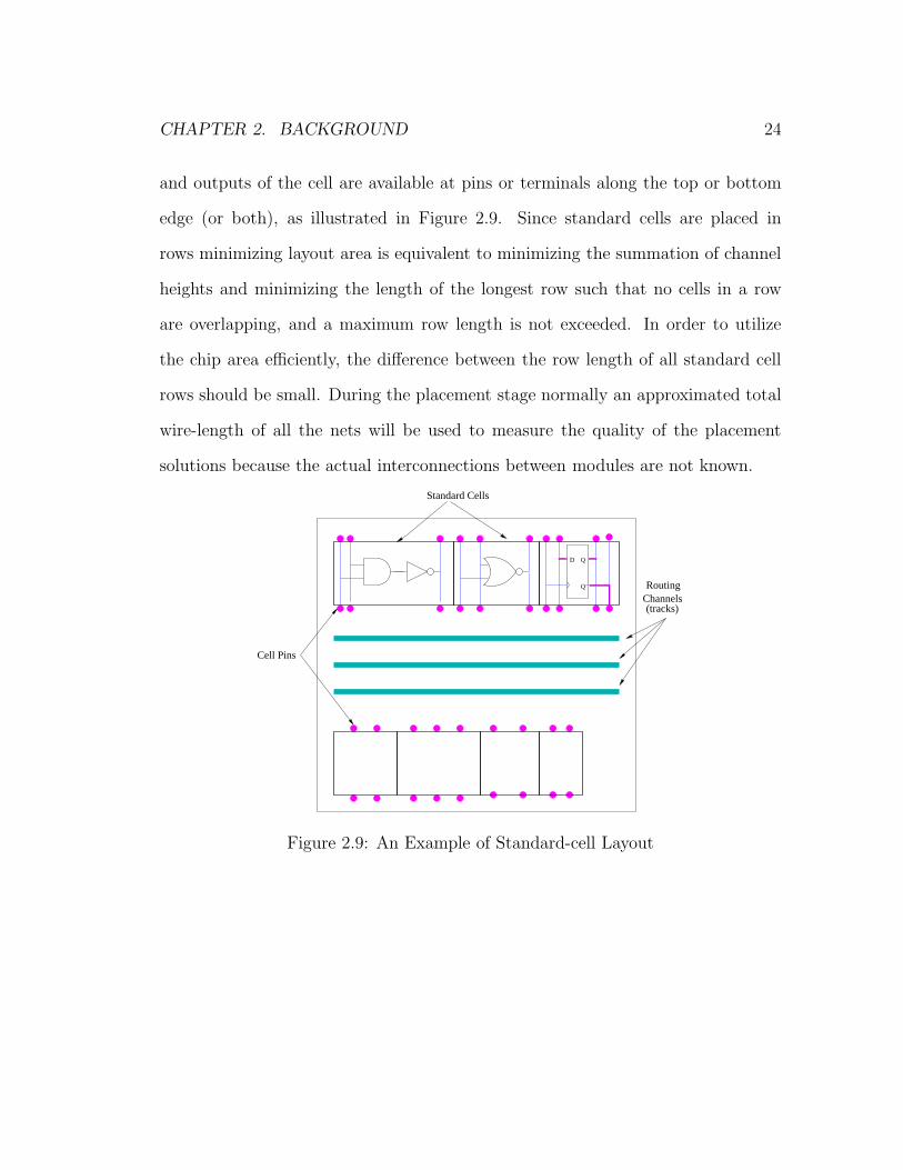
and outputs of the cell are available at pins or terminals along the top or bottom
edge (or both), as illustrated in Figure 2.9. Since standard cells are placed in
rows minimizing layout area is equivalent to minimizing the summation of channel
heights and minimizing the length of the longest row such that no cells in a row
are overlapping, and a maximum row length is not exceeded. In order to utilize
the chip area efficiently, the difference between the row length of all standard cell
rows should be small. During the placement stage normally an approximated total
wire-length of all the nets will be used to measure the quality of the placement
solutions because the actual interconnections between modules are not known.
Standard Cells
Cell Pins
(tracks)ChannelsRouting
D
Q’
Q
Figure 2.9: An Example of Standard-cell Layout

CHAPTER 2. BACKGROUND 25
2.4.2 Traditional Quadratic Measure
Usually, a circuit is represented by a hypergraph G(V,E), where the vertex set
V = {v1, v2, · · · , vn} represent the nodes of the hypergraph (set of cells to be placed),
and E = {e1, e2, · · · , em} represents the set of edges of the hypergraph (set of nets
connecting the cells). The two dimensional placement region is represented as an
array of legal placement locations. The hypergraph is transformed into a graph
(a hypergraph with all hyperedge sizes equal to 2) via clique model for each net.
Each edge ej is an order pair of vertices with a non-negative weight wj assigned
to it. The placement task seeks to assign all cells of the circuit to legal locations
such that cells do not overlap. Each cell i is assigned a location (xi, yi) on the
XY-plane. The cost of an edge connecting two cells i and j with locations (xi, yi)
and (xj, yj) is computed as the product of the squared l2 norm of the difference
vector (xi − xj, yi − yj) and the weight of the connecting edge wij. The total cost,
denoted φ(x, y), can then be given as the sum of the cost over all edges; i.e:
φ(x, y) =∑
1≤i<j≤N
wij[(xi − xj)2 + (yi − yj)
2] (2.1)
Minimizing (2.1) produces a placement with a great amount of overlap among
the cells because it attracts cells sharing common nets. Formulation (2.1) can be
rewritten in matrix form as:
φ(x, y) =1
2xTCx + dT
x x +1
2yTCy + dT
y y + t (2.2)
Vectors x and y denote the coordinates of the N movable cells; matrix C is the
Hessian matrix; vectors dTx and dT
y and the constant term t result from the contri-

CHAPTER 2. BACKGROUND 26
butions of the fixed cells. Normally the first moment constraints are added to force
the distribution of the cells to be uniform around the center of the placement area.
It follows that the quadratic placement model is given as:
Min φ(x, y)
s.t. Axx = bx
Ayy = by
lx ≤ xi ≤ ux
ly ≤ yi ≤ uy
where Ax and Ay are q × n matrices; q is the number of regions into which the
placement area has been partitioned. The q × 1 vectors bx and by represent the
centers of the q regions. The parameters lx, ux, ly and uy are lower and upper
bounds on the x and y coordinates of the cells. Clearly, the above optimization
problem can be split into two 1-dimensional subproblems and each subproblem can
then be solved independently.
2.4.3 Placement Cost Functions
Every placement method depends on the evaluation metric employed to measure
the goodness of the technique. There are three primary objectives in the automated
placement problem: minimizing chip area, achieving routable designs, and improv-
ing circuit performance. For the standard-cell layout style, since the total chip area
is approximately equal to the area of the modules plus the area occupied by the
interconnect, minimizing the wire-length is approximately equivalent to minimizing
the chip area [Shah91].

CHAPTER 2. BACKGROUND 27
Another important criterion for an acceptable placement is that it should ensure
the routability of the layout (also called congestion minimization) [Sher93a]. With
the maturity of sub-micron technology, complex circuits consisting of millions of
transistors and four to six layers of metal can now be realized on a single chip. For
these circuits, routability becomes very important issue that needs to be considered
during the placement phase, otherwise subsequent routing can become difficult and
inefficient. The work in this thesis mainly focus on wire-length and congestion cost
functions. The congestion metric will be introduced in Chapter 4.
Total Wire Length Estimation
It is computationally expensive to determine the exact total wire-length for all the
nets at the placement stage. As a result, the total wire-length is approximated
during placement. To make a good estimate of the wire-length, we should consider
the way in which routing is actually done by routing tools. Almost all automatic
routing tools use Manhattan geometry; that is, only horizontal and vertical lines
are used to connect any two points. (i.e. two layers are used such that horizontal
lines are allowed in one layer and vertical lines in the other). The shortest route
for connecting a set of pins together is a Steiner tree [Shah91] (Figure 2.10a). In
this method, a wire can branch at any Steiner point along its length so that the
total route is minimum. This method is usually not used by routers, because it
is NP-hard and the complexity of computing both the optimum branching point,
and the resulting optimum route from the branching point to the pins is high. In-
stead minimum spanning tree connections and chain connections are used. Minimal
spanning tree (Figure 2.10b) connections allow branching only at the pin locations.

CHAPTER 2. BACKGROUND 28
Hence, the pins are connected in the form of the minimal spanning tree of a graph.
Chain connections (Figure 2.10c) do not allow any branching at all. Each pin is
simply connected to the next one in the form of a chain. These connections are even
simpler to implement than spanning tree connections, but they result in slightly
longer interconnects. Source-to-sink connections (Figure 2.10d) where the output
of a module is connected to all the inputs by separate wires, are the simplest to
implement. However, they result in excessive interconnect length and significant
wiring congestion and hence, this type of connection is seldom used.
(a) Steiner Tree
Rectilinear Length = 14
(b) Minimum Spanning Tree
Rectilinear Length = 16
(c) Chain
Rectilinear Length = 17
(d) Source-to-Sink
Rectilinear Length = 24
Figure 2.10: Interconnection Topologies
An efficient and commonly used method to estimate the wire-length is the semi-
perimeter method [Sech86]. The wire-length in this method is approximated by half
the perimeter of the smallest bounding rectangle enclosing all the pins (Figure 2.11).
For Manhattan wiring, this method gives the exact wire-length for all two-terminal
and three-terminal nets, provided that the routing does not overshoot the bounding
rectangle. For nets with more pins and more zigzag connections, the semi-perimeter

CHAPTER 2. BACKGROUND 29
wire-length underestimates the actual wire-length. However, this method provides
a good estimate for the most efficient wiring scheme, the Steiner tree. The error
will be larger for minimal spanning trees and still larger for chain connections. In
practical circuits, however, two and three terminal nets are most common, and thus
the semi-perimeter wire length is considered to be a good estimate [Shah91].
HPWL
Pin
Module
Bounding Box
Figure 2.11: Wirelength Estimation by Bounding Box
Overall Cost Function
The overall cost function for standard-cell placement usually consists of three parts
[Sech88]:
COST = costwl + costovershoot + costoverlap (2.3)
1. The costwl is the total half-perimeter wirelength of all nets.
2. The costovershoot is the row length penalty function.
3. The costoverlap is the overlap penalty function.

CHAPTER 2. BACKGROUND 30
2.5 Hierarchical Placement Approach
As the complexity of VLSI circuits increases, a hierarchical improvement approach
becomes essential to shorten the design period [Hage92]. Circuit clustering plays a
fundamental role in hierarchical designs. Identifying highly connected components
in the netlist can significantly reduce the complexity of the circuit and improve the
performance of the design process.
This approach was first applied to the linear placement problem in 1972 with
Scheduler and Ulrich’s paper [Schu72] and has since been applied heavily to the par-
titioning problem. Only recently has it been applied to the standard-cell placement
problem, and then only in limited usage [Sun95, Mall89].
clusters fromedfrom cells inprevious level
A B
C D
cluster
Level 1
Level 2
Level 0
clusterde−cluster
A B
C D
de−cluster
X
Y
(Flat)
Figure 2.12: Multilevel Clustering Hierarchy.
Early methods of clustering performed the desired circuit size reduction in a
single level (e.g. [Mall89]). Research has recently shown that clustering in steps
(illustrated in Figure 2.12), reducing the circuit size gradually by adding interme-

CHAPTER 2. BACKGROUND 31
diate levels to the hierarchy, produces superior results by permitting more gradual
de-clustering [Kary97]. This gradual clustering is often called “multi-level” or
“hierarchical” clustering.
Multi-level clustering is a two-step procedure, first proceeding bottom-up, and
then top-down. The bottom-up technique is clustering, and involves the grouping
of highly connected cells into clusters and clusters into larger clusters, while the
goal of the top-down method is to determine the location for all the clusters, and
then the location of all cells within those clusters [Mall89]. The goal of this is
to reduce the number of entities that need to be improved, and the number of
interconnections between them, through the bottom-up stage. This reduces the
search space by reducing the degrees of freedom for cell moves, making a top-down
method more feasible [Arei01c]. During de-clustering in a single clustering level
heuristic, the difference between positions in clustered cells and flat circuit cells
can be substantial, and significant iterative improvement is necessary to achieve a
high quality solution. In a multi-level heuristic, much smaller differences are created
between levels of the hierarchy, because it is built slowly. During de-clustering, these
differences are more easily managed by simple interchange heuristics, resulting in
a superior quality solution in a shorter amount of time [Arei01b].
2.6 Approaches for the Standard-Cell Placement
It has been shown that circuit placement problem is NP-Complete, therefore, it
cannot be solved exactly in polynomial time [Blan85, Dona80]. Trying to get an
exact solution by evaluating every possible placement to determine the best one

CHAPTER 2. BACKGROUND 32
would take time proportional to the factorial of the number of modules. To search
through a large number of candidate placement configurations efficiently, a heuristic
algorithm must be used [Arei01a].
2.6.1 Wirelength-driven Placement Approaches
Wirelength-driven placement has been extensively studied, since traditional place-
ment approaches mainly focus on minimizing total wire-length to obtain better
routability and smaller layout area. There are a number of established approaches
for it. Depending on the input, the wire-length-driven placement algorithms can
be classified into two major classes: constructive placement methods, and iterative
improvement placement methods, as shown in Figure 2.13. The typical approach in
placement is to construct an initial solution by using constructive placement heuris-
tic algorithms. A final solution is then produced by using iterative improvement
techniques where a modification is usually accepted if a reduction in cost occurs,
otherwise it is rejected.
2.6.1.1 Constructive Placement
Constructive placement produces a complete placement from a partial or non-
existent placement. It takes a negligible amount of computation time compared
to iterative improvement placement and provides a good starting point for them
[Shah91]. However, the solution generated by constructive algorithms may be far
from optimal. Thus, an iterative improvement placement algorithm is performed
next to improve the solution. Usually, constructive placement algorithms include
cluster growth, numerical optimization, partitioning-based placement [Gare79], and
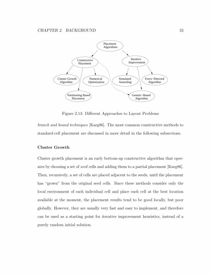
CHAPTER 2. BACKGROUND 33
AlgorithmsPlacement
Constructive Placement Improvement
Iterative
AlgorithmCluster Growth
OptimizationNumerical Force−Directed
Algorithm
PlacementPartitioning Based Genetic−Based
Algorithm
AnnealingSimulated
Figure 2.13: Different Approaches to Layout Problems
branch and bound techniques [Karg86]. The most common constructive methods to
standard-cell placement are discussed in more detail in the following subsections.
Cluster Growth
Cluster growth placement is an early bottom-up constructive algorithm that oper-
ates by choosing a set of seed cells and adding them to a partial placement [Karg86].
Then, recursively, a set of cells are placed adjacent to the seeds, until the placement
has “grown” from the original seed cells. Since these methods consider only the
local environment of each individual cell and place each cell at the best location
available at the moment, the placement results tend to be good locally, but poor
globally. However, they are usually very fast and easy to implement, and therefore
can be used as a starting point for iterative improvement heuristics, instead of a
purely random initial solution.

CHAPTER 2. BACKGROUND 34
Numerical Optimization
One constructive placement approach is numerical optimization. In these methods,
the original standard-cell placement problem is approximated by a similar problem
that can be solved in polynomial time [Thom00]. That is, the placement objec-
tive function is approximated by a mathematical formulation. The formulation is
then solved exactly using mathematical programming techniques such as linear,
non-linear, integer, and dynamic programming techniques [Behj98]. The solution
produced by minimizing this formulation are good from a “global” perspective, but
are sub-optimal according to the actual chip layout, since such a formulation does
not restrict cells to occupy legal position and therefore, result in high overlap among
the cells. To get a legal solution, a legalization heuristic must be used to find a
“good” legal position for each cell. Many methods have been used to approximate
the exact standard-cell problem, the most popular being linear models [JMK91]
and quadratic programming models [Chen84, Behj98, Etaw99b].
Numerical methods are never used alone due to the errors introduced by the le-
galization process. Usually, search techniques are used after the numerical methods
to further improve the quality.
Partitioning-based Placement
Another popular constructive approach is partitioning-based placement which is
an important class of placement algorithms based on repeated division of the given
circuit into densely connected sub-circuits such that the number of nets cut by
the partition is minimized. In an early algorithm, Breuer [Breu77a, Breu77b] uti-

CHAPTER 2. BACKGROUND 35
lized repeated graph bisections to obtain a circuit placement. With each bisec-
tion, the vertices (cells) were assigned to progressively smaller regions. Dunlop
and Kernighan [Dunl85] extended this approach, through the use of an improved
partitioning method [Kern70], and also terminal propagation. Unlike partitioning
algorithms, placement algorithms which are based on partitioning need to consider
not only the internal nets of the subcircuit but also the nets connected to external
modules at higher levels of the hierarchy. Terminal propagation provides a simple
method to insert fixed “dummy” vertices, so that the partitioning considers these
external connections.
Moving beyond simple bisections, Suaris and Kedem [Suar88] explored the use
of quadrisection (a four way partitioning). Huang and Kahng [Huan97] also apply
quadrisection, utilizing a multi-level clustering based partitioning algorithm, and
considering minimum spanning tree lengths, rather than the simple min-cut metric.
Besides, the large scale multi-way partitioning placement approaches that allows
the consideration of global objectives are presented in [Zhon00, Yild01].
Like numerical optimization methods, partitioning-based methods do not di-
rectly attempt to minimize wire-length, and so the solution obtained is sub-optimal
in terms of wire-length. Search heuristics are used to further improve the solution.
2.6.1.2 Iterative Improvement
An iterative improvement heuristic starts with an initial placement solution, and
attempts to improve it by repeatedly modify it. Better solutions are obtained
by perturbing the solution in some way in order to find a cost reduction. Al-
though iterative improvement placement methods can produce a good placement,

CHAPTER 2. BACKGROUND 36
the computation time of such algorithms is also large. Therefore, the heuristics
rely immensely on efficient constructive placements. There are two classes of itera-
tive improvement placement methods: Deterministic and Stochastic heuristics. A
deterministic heuristic interchanges randomly selected pairs of modules and only
accepts the interchange if it results in a reduction in cost [Goto76]. While it is fast,
it gets trapped in a local minimum quickly due to its characteristic. In contrast, a
stochastic heuristic not only accepts the possible perturbation that results in cost
reduction but also uses some “randomness” to accept some poor solution, which
allows the heuristic to avoid the local-optimal and explore the solution space more
effectively. In the following subsections, the most common approaches of iterative
improvement are presented.
Interchange Methods
The interchange methods, such as Pairwise Interchange, Force-Directed Interchange,
are the simplest iterative improvement methods. It swaps the randomly selected
pairs of modules and accepts the interchange if it results in a cost reduction. An
example of pairwise interchange is shown in Figure 2.14. Obviously, such an algo-
rithm is a deterministic heuristic, since it only accepts moves that reduce the total
cost.
Simulated Annealing
In 1983, a new algorithm technique—Simulated Annealing is presented in [Kirk83].
The idea of simulated annealing is originated from the observation of crystal for-
mation. When a material is heated, the modules move around randomly. When

CHAPTER 2. BACKGROUND 37
Pairwise Interchange Type (b)Pairwise Interchange Type (a)
Figure 2.14: Pairwise Interchange
the temperature slowly decreases, the modules move less and finally form a crys-
tal structure. The cooling process is done more slowly, the crystal lattice is more
stronger. The simulated annealing technique has been successfully used in many
phases of VLSI physical design, including circuit placement. Many implementa-
tions of simulated annealing have been applied to the standard-cell problem (e.g.,
[Sech87, Mall89, Sun95]).
The basic procedure in simulated annealing is to start with an initial placement
and accept all perturbations or moves which result in a reduction in cost. Moves
that result in a cost increase are accepted with a probability that decreases with
the increase in cost. A parameter T, called the temperature, is used to control the
acceptance probability of the cost- increasing moves [Shah91].
Obviously, simulated annealing is a stochastic method with hill-climbing ability.
The cooling schedule(ie. the rate of temperature change) determines the quality of
the final solution. Simulated annealing is one of the most established algorithms
for placement problems. It produces good quality results when given a long-enough
time and a good cooling schedule but the computation time is also large. Therefore,
it is only suitable for small to medium sized circuits.

CHAPTER 2. BACKGROUND 38
Genetic based Placement
Genetic algorithms (GA’s) which were introduced by Holland in the 1970s [Holl75],
are a class of optimization algorithms based on the mechanics of natural selection
and natural genetics. They combine the use of string codings and populations with
the power of reproduction and recombination to motivate a surprisingly powerful
search heuristic in many problems. GA’s have been applied to various domains,
including image processing, pipeline control system, machine learning and combina-
tional optimization. In [Coho86], the genetic algorithm was first applied to circuit
placement problem and have been proved a promising placement technique.
The simple Genetic Algorithm starts with an initial set of random solutions,
called a population. A solution string (called a chromosome) is encoded as a binary
or integer string. During each iteration, called a generation, each individual in
the current population is evaluated and assigned a fitness value through a scoring
function. Based on this fitness, individuals are selected for reproduction and their
chance for selection increases with their fitness. A number of genetic operators
are then applied to the parents to generate new individuals, called offsprings. The
commonly used genetic operators are crossover and mutation. A new generation is
formed by selecting the individuals from the parents and offspring according to their
fitness so that the population size can be kept constant. Over many generations, the
fitter individuals tend to predominate the population while the less fit individuals
tend to die-off and eventually one super-fit individual evolve. A detailed explanation
of GA will be introduced in chapter 3

CHAPTER 2. BACKGROUND 39
Iterative Force-Directed Improvement
Force-directed placement explores the similarity between the placement problem
and the classical mechanics problem of a system of bodies attached to springs
[Sher93a].
Starting with an initial solution, this method assumes the cells that are con-
nected by nets exert an attractive force on each other. The magnitude of the force
between any two cells is directly proportional to the distance between the two cells.
When a cell is considered for a move, it is moved in the direction of the total force
exerted on it until this force is zero. This method can be implemented to run
quickly, and has shown to perform well. However, determining the weight function
for each net is difficult, and varies from circuit to circuit.
2.6.2 Generating a Legal Placement
Solving the numerical optimization problem produces an optimal solution according
to a mathematical model of the system, but sub-optimal solution according to the
actual chip layout. This is because the solution does not put cells in slots (cells are
confined to the center of the region), while in standard-cell layout cell positions are
constrained to non-overlapping position in a row. Besides, the solutions generated
by other placement methods, such as partitioning-based placement may have cell
overlaps within a row. Therefore, a legalization heuristic should be used to find a
legal position for each cell after these placement approaches.
A good legalizer should not only legalize the solution but also minimize the
difference in wirelength between the original solution and the legalized solution.

CHAPTER 2. BACKGROUND 40
Figure 2.15 shows an approach (uniform mapping) for generating the legal place-
ment, suggested in [Song92].
83
6
9
2
4
7
1
5
(a) Initial Solution
8 1
2 67
5
4
9
3
(b) Uniform Legalization
13
2
76 5
94
8
(c) After Legalization
13
2
76 5
9
8
4
(d) Remove Cell Overlaps
Figure 2.15: Placement Legalization
Figure 2.15 (a) shows the position of cells after the numerical optimization
based placement. Uniform mapping method attempts to move cells to the slots
that are close to their locations so that the routing can ultimately be performed
easily, but it could also generate an overlapping placement, as shown in Figure
2.15(b) and (c). One way to overcome this problem is to resort to a heuristic to
remove all the overlaps while keeping the total half perimeter wire length as short as
possible (shown in Figure 2.15(d)). In addition, since optimality deteriorates when
legalizing the placement solution, iterative improvements have to be performed after
legalization to regain some of the lost optimality.

CHAPTER 2. BACKGROUND 41
2.7 Test Circuits
Table 2.1 and 2.2 show the general information of benchmark circuits used to mea-
sure the performance of the heuristics in this thesis. The circuits used are the
MCNC’91 benchmarks [Kozm91]. This test set consists of ten circuits ranging in
size from 125 cells to over 25,000 cells.
The second column of Table 2.1 shows the number of cells within the circuit.
The third column indicates the pads (i.e I/O connections) that connect the circuit
to the outside world. The fourth column presents the number of nets connecting the
cells within the benchmarks. The total number of pins (i.e connections) within the
circuit is summarized in column five. The sixth column gives the number of rows
where the cells are to be placed (exclusively for the circuit placement problem).
The “Pad Distribution” column indicates the number and location of pads. Table
2.2 shows the net and cell distribution of different benchmarks. The first part
of this table “Nets Incident on Cell” lists the percentage number of cells on one
net, two nets, three nets, four nets and five more nets. The second part “Cells
Incident on Net” shows the percentage number of nets with two cells, three cells,
four cells, and so on. It is important to notice that these benchmarks have different
characteristics.
The circuit have been grouped into three categories according to size: small,
medium, and large, as indicated by the horizontal lines in Table 2.1. This classifi-
cation will be used in the entire thesis to illustrate the effectiveness of the heuristic
techniques developed. The performance of wirelength-driven placement is measured
by total wirelength for all the nets and computation time, while the performance

CHAPTER 2. BACKGROUND 42
of congestion-driven placement is measured by overflow, total wirelength and com-
putation time. All the results shown in this thesis are the average of 5 runs. The
proposed optimization techniques are implemented in the ‘C’ programming lan-
guage on a Sun Ultra10 workstation.
Circuit Cells Pads Nets Pins Rows Pad DistributionTop Bottom Left Right
Fract 125 24 147 462 6 22 2 0 0Prim1 752 81 904 5526 16 21 20 20 20Struct 1888 64 1920 5471 21 64 0 0 0
Ind1 2271 814 2478 8513 15 254 258 302 0Prim2 2907 107 3029 18407 28 30 16 30 31Bio 6417 97 5742 26947 46 8 72 9 8
Ind2 12142 495 13419 125555 72 107 126 123 139Ind3 15059 374 21940 176584 54 113 124 63 74
avq.small 21854 64 22124 82601 80 30 34 0 0avq.large 25114 64 25384 82751 86 30 34 0 0
Table 2.1: MCNC Benchmarks Used for Testing
Circuit Nets Incident on Cell Cells Incident on Net1 2 3 4 ≥ 5 2 3 4 5-19 ≥ 20
Fract 16% 27% 24% 8% 24% 47% 30% 10% 19% 0.0%Prim1 5.6% 18% 25% 33% 19% 55% 26% 6.9% 12.1% 0.0%Struct 4% 24% 61% 12% 0.0% 39% 60% 0.0% 1.6% 0.0%
Ind1 1.5% 21% 35% 20% 21% 65% 16% 5.5% 12.9% 0.6%Prim2 1.4% 15% 42% 17% 23% 61% 12% 6.7% 19.9% 0.4%Bio 0.03% 13% 70% 6.9% 10% 69% 16% 7.5% 5.3% 2.2%
Ind2 1.3% 21% 24% 29% 24% 71% 14% 2.3% 11.5% 1.2%Ind3 0.1% 5.8% 27% 21% 46% 57% 23% 8.5% 11.2% 0.3%
avq.small 0.29% 24% 42% 12% 20% 62% 28% 7% 3.3% 0.01%avq.large 0.25% 21% 62% 1% 17% 67% 24% 6% 3.5% 0.01%
Table 2.2: Statistical Information of MCNC Benchmarks

CHAPTER 2. BACKGROUND 43
2.8 Summary
The VLSI design process is broken down into several smaller and tractable sub-tasks
to manage the high complexity of the task. One of these sub-tasks is physical design,
which is still incredibly complex. As a result, this complexity is handled by dividing
the physical design task into more tractable sub-tasks and circuit placement is one
of such sub-tasks. Physical design automation highly depends on the layout style
used. Different layout styles, such as full-custom, gate-array, and standard-cell
layouts can achieve different tradeoffs among speed, cost, fabrication time, and
degree of design automation.
The layout topology used to demonstrate the research work in this thesis is
the standard-cell layout style. The most commonly used metric that measures the
quality of a placement solution is total wire-length for all the nets and many place-
ment approaches have been taken to solve wire-length-driven placement problem
[Shah91], including constructive and iterative improvement methods.
In the following chapters several heuristic based techniques are implemented to
solve the circuit placement based on both wirelength and congestion.

Chapter 3
Mathematical/Heuristic Based
Approaches
3.1 Introduction
The layout of integrated circuits on chips is one of many interrelated complex tasks
in VLSI circuit design. Placement is a sub-problem of circuit layout which is usually
subdivided into an initial placement phase (global/constructive placement) and an
iterative improvement phase (detailed placement). Placement solutions produced
by initial placers will largely influence the convergence of iterative improvement
placement techniques. In this Chapter, the performance of several constructive
placement methods based on (i) Random Placement (ii) Cluster Development (iii)
Bipartitioning Based Algorithms (iv) Quadratic Based Placement are introduced
and compared. The Cluster Development approach is a simple greedy adaptive con-
structive technique whereas Bipartitioning is assumed to be Meta-Heuristic tech-
44

CHAPTER 3. MATHEMATICAL/HEURISTIC BASED APPROACHES 45
nique that is suitable for constructing good initial solutions. The quadratic based
placement minimizes a certain quadratic net-length estimation and provides good
relative placement with overlaps (a legalization phase follows to produce feasible
solutions as explained in Chapter 2). Both flat and hierarchical approaches are used
to find the effectiveness of these approaches. An iterative improvement approach
follows the initial placement produced by each technique and the robustness is mea-
sured in terms of both the wirelength and CPU time consumed by the constructive
and local heuristics. In addition, an evolutionary based technique is developed to
explore the solution space effectively.
Section 3.2 introduces the different constructive placement algorithms imple-
mented in this thesis. In section 3.3, a Tile-based iterative improvement method
and a multi-level clustering approach are explained. The experimental results pro-
duced by these different constructive methods are then presented in section 3.4.
Section 3.5 presents an evolutionary algorithm and the corresponding experimental
results. This Chapter concludes with a summary.
3.2 Constructive Placement Algorithms
3.2.1 Attractor Repeller Placer
The Attractor Repeller Placer (ARP)[Etaw99b] is basically broken down into a
relative placement phase followed by legalization and improvement phases. The
traditional wirelength formulation is extended by adding a repelling term such that
upon minimization, a target distance is maintained between the locations of cells
sharing common signals. It also adds attracting forces to pull cells from dense

CHAPTER 3. MATHEMATICAL/HEURISTIC BASED APPROACHES 46
to sparse regions resulting in a uniform distribution of the cells on the placement
area. Figure 3.1 illustrates cell spreading based on the AR (Attractor and Re-
peller) model. Figure 3.1(a) shows the initial solution obtained from minimizing
the quadratic wirelength. Clearly, the majority of the cells are located in the center
of the placement area and the amount of overlap between the cells is substantial.
The cell attractors (shown as circles in the figure) are created according to the
current cell positions. Figure 3.1(b-d) illustrate the spreading after including the
cell attractors and repellers. It can be seen that better spreading of the cells can
be achieved in each iteration compared to the preceding iterations.
(a) (b)
(c) (d)
++++
+
+
++++++
+++ ++++++++
++
++++
++
Figure 3.1: Effect of the Repellers and Attractors (“+”represents locations of mov-able cells, “X” represents location of I/O pads on the chip periphery, and “o”represents locations of attractors).
The formulations of ARP are convex and neither partitioning nor hard con-
straints are used. Moreover, they are versatile in the sense that they are applicable

CHAPTER 3. MATHEMATICAL/HEURISTIC BASED APPROACHES 47
to a variety of problems where a target distance is desired between connected com-
ponents [Etaw99b].
Mathematical Formulation
As indicated in Chapter 2 section 2.4.2, minimizing the quadratic model for wire-
length yields a placement where cells overlap. Consequently, extra efforts need to
be done to remove the overlap. In all previous attempts, the overlap problem is
handled by partitioning the placement area and changing the constraints on cell
locations before solving another optimization problem. An intuitive idea to avoid
partitioning is to maintain a target distance between each connected pair of cells.
In other words, place the cells such that a lower bound on the distance between
their respective locations is maintained. For example, the following formulation
accomplishes this aim, Du and Vannelli [Du98].
ψ(x, y) =∑
1≤i<j≤N
wij[(xi − xj)2 + (yi − yj)
2 − dij]2 (3.1)
Minimizing (3.1) yields a placement with no overlap between connected cells.
However, this model is not convex, and thus convergence to a global optimal answer
is not guaranteed.
In the ARP algorithm, the convex repeller model for the pair of connected cells
i and j is as follows:
f(zij) =
η(zij) if zij ≥ 1
0 otherwise(3.2)
where η(zij) = zij+ρ(zij) and ρ(zij) ∈ {−ln(zij) − 1, e1−zij − 2}. zij =(xi−xj)
2+(yi−yj)2
d.
The full Attractor-Repeller model for the global placement can then be given as:

CHAPTER 3. MATHEMATICAL/HEURISTIC BASED APPROACHES 48
Minf(z) + g(x) + h(y) (3.3)
s.t. lx ≤ xi ≤ ux
ly ≤ yi ≤ uy
Parameter lx, ly, ux and uy are lower and upper bounds on x and y. The first term,
f(z), represents the repelling terms. The second and the third terms, g(x) and
h(y), represent the attracting terms.
Basic Algorithm
Figure 3.2 illustrates the flow of the ARP algorithm. Throughout the remaining
Global Optimization:
Global Optimization:
Stopping criteria issatisfied
Cell-Attractor Assignment:
Stopping criteria isnot satisfied
(QP model)
closest attractorimprove placement slightly and assign each cell to
Attractor-Repeller (AR) model
circuit informationInput:Output:
legal placement
Create Attractors:cell distributionbased on current
. Update AR model accordingly.
Figure 3.2: An Outline of the Placement Procedure ARP.
parts of this thesis, we refer to the new placement method as ARP (Attractor
Repeller Placer). Following the parsing circuit description, an initial placement is
determined using the quadratic formulation of the wirelength. In the subsequent

CHAPTER 3. MATHEMATICAL/HEURISTIC BASED APPROACHES 49
iterations, the algorithm proceeds iteratively by solving the AR model. In each
iteration, cells move to fill sparse regions and better spreading of the cells over the
placement floor is achieved. In a subsequent iteration, current attractors are deleted
and new ones are created; the AR-model is updated accordingly. This process
continues until the algorithm reaches a point where no significant movement of the
cells is attained. The algorithm stops when a maximum number of iterations K is
exceeded, or if the ratio of the total area of sparse regions to that of the placement
area is < κ%. Experimentally, the authors of [Etaw99b] found that 5 ≤ K ≤ 10
and κ = 10% are quite sufficient to uniformly spread the cells over the placement
area and achieve good wirelength. One of the main objectives of this thesis is to
utilize the ARP technique at the hierarchical placement stage versus the flat stage
as has been done in [Etaw99b]. Several parameters are adjusted to accommodate
the clustering of cells into sub-clusters.
3.2.2 Cluster-Seed Based Placement
Cluster-Seed placement is a constructive (cluster growth) placement algorithm that
is capable of producing a good initial solution. Cluster growth placement is a
bottom-up method that operates by selecting modules and adding them to a partial
placement [Karg86]. Normally, it contains two functions: (i) selection function and
(ii) placement function. The selection function determines the order in which the
unplaced modules are included in the layout of the chip. The order is a function
of the connectivity between modules. The placement function decides the best
position for the modules according to the availability of vacant space in the region
[Karg86].

CHAPTER 3. MATHEMATICAL/HEURISTIC BASED APPROACHES 50
Figure 3.3 shows a simple circuit to be placed using the Cluster-Seed based
method. First, a seed placement is determined by selecting the pads in a random
In2A
In3
In4
(b) Cluster−Seed Placement(a) Input Nellist
1 3
4
5
62
OutputA
In2
In3
In4
In15 36 1
42
In1
Figure 3.3: An Example of Cluster-Seed Based Placement Algorithm
order and placing those unplaced modules that are directly connected with these
pads. Next, other unplaced modules are selected one at a time in order of their
connectivity to the placed modules (highly connected first) and fixed at a vacant
position close to the placed modules so that the total wire length is minimized.
This step is repeated until all the modules are placed. The Cluster-Seed based
placement algorithm is described in Figure 3.4.
In order to place modules uniformly on the chip (thereby minimizing the chip
area and total row length), an adaptive placement function is utilized in the current
implementation. For Benchmarks that do not have pads at bottom or top of the
chip, a Top-pads-placement() function or Bottom-pads-placement() function is used
respectively. In these two functions, modules are placed in top-down, or bottom-up
fashion respectively so that the modules are uniformly spread out. For circuits
that have both bottom and top pads, a normal-pads-placement() function is used.

CHAPTER 3. MATHEMATICAL/HEURISTIC BASED APPROACHES 51
CLUSTER-SEED ALGORITHM1. Read Benchmark;2. Set Total mods, placed mods;3. Place the modules connecting with the
pads directly and update placed mods;4. While (placed mods 6= Total mods)
If (all the pads on the top side)Top pads placement();
Elseif (all the pads on the bottom side)Bottom pads placement();
ElseNormal pads placement();
update placed modsEnd While
5. Return the legalized placement solution.
Figure 3.4: A Cluster-Seed Based Constructive Algorithm
Initially, the chip area is partitioned into four equal subregions. Next, modules are
placed by different ways according to the subregions they belong to such that these
modules are spread out evenly. In the final stage, a legalizing function is used to
remove the cell overlap.
3.2.3 Partitioning Based Placement
The netlist partitioning problem can be formulated as a hypergraph H(V,E), with
n vertices V = {v1, v2, ...vn}. Each edge ei ∈ E of the hypergraph connects a subset
of the vertices. The objective is to partition the hypergraph into subsets such that
we minimize the total number of cut edges, while meeting constraints on the total
number of vertices in each partition. The survey of Alpert and Kahng[Alpe95a]
provides four general classifications for current approaches to the traditional par-
titioning problem: Move-Based approaches, Geometric approaches, Combinatorial

CHAPTER 3. MATHEMATICAL/HEURISTIC BASED APPROACHES 52
Formulation approaches and Clustering approaches. The move-based approaches
frequently employ iterative improvement, in which an initial partition is optimized
by repeatedly moving a vertex from one cluster to another, or by swapping pairs
of vertices. Kernighan and Lin (KL) [Kern70] proposed a two-way graph parti-
tioning algorithm which became the basis for most of the subsequent partitioning
algorithms. The approach for placement can be summarized as follows: we initially
obtain a placement for the benchmark using a cluster seed approach. We then
follow this with a multi-way partitioning scheme that reduces the number of cuts
between the blocks (i.e rows for the placement problem). A simple optimization
technique follows to place each row optimally within the chip and with respect to
the other rows.
Figure 3.5 shows the Multi-Way partitioning based placement algorithm. First
an initial placement is generated by Random placement or ClusterSeed placement.
Next the multi-way partitioning stage is invoked, where the whole chip is partitioned
into several blocks equal to the number of rows. A move based partitioning approach
is used to minimize the nets cut between the rows. Since the partitioning based
placement does not directly attempt to minimize the total estimated wirelength,
a simple row-based optimization technique is used to optimize the total estimated
wirelength of the solution.

CHAPTER 3. MATHEMATICAL/HEURISTIC BASED APPROACHES 53
Multi-Way Partitioning
the netcuts between these bolcksblocks and then moving cells to minimizepartitioning thc chip area into several
Technique
placement solution circuit information
Row based Optimization Initial Placement
Random / ClusterSeed
Input:Output:
Figure 3.5: A Multi-Way Partitioning Based Placement Algorithm
3.3 Clustering & Iterative Improvement Techniques
3.3.1 Weighted Hyper-edge Clustering Technique
As mentioned in Chapter 2 section 2.5, multi-level clustering is an important tool
to manage the complexity of circuits with millions of transistors. In this section
we introduce a simple multi-level clustering technique called “Weighted Hyper-edge
Clustering” [Arei01c], which is an extension to Karypis et. al work [Kary97]. As
seen in the pseudo-code in Figure 3.6, an upper and lower width limit is determined
based on the cell widths in the current hierarchical level. As a potential clustering
of cells is examined, a new cluster is only created if the sum of the constituent cells’
widths is between these width limits. This limitation on sizes prevents excessively
large clusters from impeding improve, yet still reduce the problem size.
Similar to the Karypis’ MHEC method, the weighted Hyper-edge clustering
method is also divided into passes. In the first pass, for each net, cells are greedily

CHAPTER 3. MATHEMATICAL/HEURISTIC BASED APPROACHES 54
Weighted Hyper-edge Clustering Algorithm1. Read Benchmark2. Sort nets by increasing size3. For each sorted net
If no cell on net is clusteredIf sum of cell widths on net is within limits
Cluster all cells on netEnd If
End IfEnd For
4. For each sorted netIf sum of unclust cell widths is within limits
Cluster all unclust cells on netEnd IfEnd For
5. For each cell in circuitIf not clustered
Create a new cluster from cellEnd IfEnd For
6. Return the Clusted Circuit.
Figure 3.6: Weighted Hyperedge Clustering
clustered together, but only if the sum of the cell width are within width limits. In
the second pass, remaining unclustering cells on each net are also greedily clustered
together if the sum of the cell width are within width limits. Finally, since it is
possible that some cells are only connected to a cluster that is prohibited from
clustering based on its size, a third pass is performed to assign any remaining cells
to a new cluster. The whole process eliminates the huge clusters allows a large
amount of circuit size reduction. Limiting sizes in the first pass only prevents huge
clusters from forming. Therefore, the criteria for selecting size limits need not be
complex. In this implementation, twice the maximum cell width was used to limit
sizes in the first pass. This encourages at most a doubling of the maximum cell size
at each level of the hierarchy. During the De-clustering process, a greedy method for
reducing the legalization error called FLATTEN is used. To minimize the quality
deterioration during circuit flattening, further improvement is performed on the

CHAPTER 3. MATHEMATICAL/HEURISTIC BASED APPROACHES 55
circuit at each flattening stage, using a localized search heuristic.
3.3.2 Tile Based Iterative Improvement
A good placement heuristic should consider both quality and computational effi-
ciency issues. The quality of the placement is essential for the performance of the
final circuit whereas computational efficiency is essential for shortening the design
procedure. Tile based iterative heuristic is such a kind of algorithm that produces
good solutions in a reasonable amount of time [Arei01a]. In the Tile based approach,
overlapping tiles or windows [Kenn97] are introduced to localize the arrangement
of cells throughout the placement area. The introduction of tiles is useful for re-
stricting the rearrangement of cells. Each tile contains a small subset of the cells.
Furthermore, cells may belong to more than one tile due to the overlap which exists
between tiles. The Tile iterative approach works as follows. A tile is selected, and
a list of cells within the tile is generated. Subsequently, cells within the selected
tile are rearranged in some fashion. In rearranging the cells, the cells are restricted
to positions within the tile boundaries which keeps cells close to their original posi-
tions. The computational effort required to find improved cell positions is reduced,
since the search for improved cell positions is restricted to positions within the tile
boundaries. Since tiles overlap, cells near the boundaries of a tile may be permitted
to move between tiles. During one pass, tiles are selected randomly, and only once
during each pass. After each pass, the quality of the placement is evaluated and
compared to placements generated by previous passes. The algorithm terminates
when either a maximum number of passes is exceeded, or when the improvement
in the placements over a number of consecutive passes is negligible. Figure 3.7

CHAPTER 3. MATHEMATICAL/HEURISTIC BASED APPROACHES 56
summarizes the Tile approach.
TILE-BASED ALGORITHM1. Input: initial placement s;
estimate wirelength(initial placement);2. Select Tiles Randomly;3. For each Tile
While attempted moves < max attemptsselect cells i and j;determine cell shifts();estimate wirelength(new placement)if 4Total wirelength ≤ 0 doupdate placement();
End While4. Output Best placement found so far
Figure 3.7: A Tile-Based Algorithm
3.4 Results Comparison
The different constructive heuristic techniques are tested on ten MCNC bench-
marks introduced in section 2.7. The comparison is based on the total wirelength
of all the nets and computation time. The units of total wirelength and compu-
tation time are bounding box wirelength and seconds, respectively. Both flat and
hierarchical approaches are used to find the effectiveness of these approaches. An
iterative improvement approach (Tile-based Improver) follows the initial placement
produced by each technique and the robustness is measured in terms of quality of
solutions produced by the initial placement and final placements achieved using
the local search heuristic. Tables 3.1, 3.2, 3.3, and 3.4, present initial placement
results based on random placement, ARP algorithm, Cluster-Seed algorithm and
partitioning-based algorithm using both a flat level methodology and hierarchical
level approach. Table 3.1 introduces the initial wirelength for several benchmarks

CHAPTER 3. MATHEMATICAL/HEURISTIC BASED APPROACHES 57
obtained by the constructive placement techniques at the flat level. Results from
Table 3.1 indicate that initial placement based on the ARP algorithm gives the
best results for all the benchmarks at the expense of more computation time. The
clustering based results shown in Table 3.2, 3.3 and 3.4 were obtained by running
the constructive placement heuristic at clustering level 1, 2, and 3 respectively. The
constructive heuristic was only performed on the circuit at the top level. There is
no further improvement performed on the circuit at top level and succeeding flat-
tening stages. From these three tables, it can be seen that the computation time
and the quality of the solutions were improved as the clustering level increases. In
Table 3.4 (clustering depth is 3), more than 40% of the results produced by different
constructive placement algorithms were improved on average by 30%, especially for
Partitioning based placement and Random placement. In addition, the computa-
tion time of the ARP algorithm which produces the best results in Table 3.4 have
been largely reduced by 85% with a slight increase in total wirelength.
Circuit Random ARP ClusterSeed PartitioningX+Y T X+Y T X+Y T X+Y T
Fract 87823 0.1 45214 0.5 73716 0.1 55431 0.4Struct 2.49+6 0.3 705559 9.0 945343 0.2 956804 2.7Prim1 2.63+6 0.1 1.13+6 8.7 1.85+6 0.1 2.02+6 2.0
Avg 1.74+6 0.2 6.27+5 6.1 9.56+5 0.2 1.01+6 1.7
Ind1 6.20+6 0.5 2.15+6 46.4 4.91+6 0.4 4.75+6 3.7Prim2 1.64+7 0.4 5.89+6 53.7 1.22+7 0.5 1.17+7 5.6Bio 1.33+7 1.4 3.06+6 121.2 7.54+6 1.4 7.49+6 9.3
Avg 1.20+7 0.8 3.7+6 73.8 8.2+6 0.8 8.0+6 6.2
Ind2 9.29+7 3.9 2.69+7 388.1 7.19+7 4.3 6.12+7 22.0Ind3 2.82+8 6.1 6.90+7 410.7 2.08+8 6.8 1.81+8 50.5avq.s 8.80+7 14.5 1.36+7 732.7 7.38+7 17.0 5.94+7 43.6avq.l 1.02+8 16.1 1.64+7 877.5 8.64+7 21.8 6.96+7 47.9
Avg 1.41+8 10.1 3.15+7 602.1 1.10+8 12.4 9.28+7 41.0
Table 3.1: Initial Placement Solutions without Improver at Flat Level
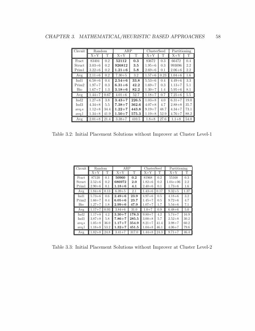
CHAPTER 3. MATHEMATICAL/HEURISTIC BASED APPROACHES 58
Circuit Random ARP ClusterSeed PartitioningX+Y T X+Y T X+Y T X+Y T
Fract 83404 0.2 52112 0.3 83672 0.3 66472 0.4Struct 3.03+6 0.2 926812 3.5 1.95+6 0.3 993096 2.2Prim1 3.22+6 0.2 1.21+6 5.8 2.69+6 0.1 2.06+6 2.2
Avg 2.11+6 0.2 7.30+5 3.2 1.57+6 0.23 1.04+6 1.6
Ind1 6.58+6 0.4 2.54+6 33.8 5.53+6 0.4 4.49+6 3.3Prim2 1.97+7 0.3 6.31+6 42.2 1.69+7 0.3 1.13+7 5.1Bio 1.67+7 1.3 3.18+6 82.2 1.30+7 1.4 5.95+6 8.1
Avg 1.44+7 0.67 4.01+6 52.7 1.18+7 0.7 7.25+6 5.5
Ind2 1.27+8 3.8 3.43+7 226.5 1.03+8 4.0 6.31+7 19.0Ind3 4.34+8 5.5 7.38+7 362.6 4.07+8 4.7 2.88+8 35.7avq.s 1.12+8 34.4 1.22+7 443.8 9.19+7 48.7 4.34+7 73.1avq.l 1.34+8 41.9 1.50+7 575.3 1.19+8 52.9 4.76+7 88.2
Avg 2.01+8 21.4 3.38+7 410.5 1.8+8 27.6 1.1+8 54.0
Table 3.2: Initial Placement Solutions without Improver at Cluster Level-1
Circuit Random ARP ClusterSeed PartitioningX+Y T X+Y T X+Y T X+Y T
Fract 87120 0.1 50960 0.2 81968 0.2 55168 0.3Struct 2.52+6 0.2 686972 2.0 1.82+6 0.2 1.01e+06 2.2Prim1 2.90+6 0.1 1.18+6 4.1 2.40+6 0.1 1.73+6 1.6
Avg 1.84+6 0.13 6.39+5 2.1 1.43+6 0.17 9.32+5 1.37
Ind1 5.73+6 0.6 2.49+6 23.9 4.97+6 0.5 4.18+6 3.2Prim2 1.66+7 0.4 6.05+6 23.7 1.45+7 0.5 9.72+6 4.7Bio 1.27+7 1.8 2.99+6 47.9 1.07+7 1.7 5.54+6 7.1
Avg 1.17+7 0.93 3.84+6 31.0 1.0+7 0.9 6.48+6 5.0
Ind2 1.17+8 4.2 3.30+7 178.3 9.80+7 4.2 5.74+7 16.9Ind3 3.87+8 5.8 7.86+7 285.5 3.00+8 5.7 2.52+8 30.2avq.s 1.05+8 36.0 1.17+7 354.9 8.21+7 41.4 3.98+7 60.2avq.l 1.18+8 53.2 1.32+7 451.5 1.04+8 46.1 4.06+7 79.6
Avg 1.82+8 24.8 3.41+7 317.0 1.44+8 24.3 9.71+7 46.4
Table 3.3: Initial Placement Solutions without Improver at Cluster Level-2

CHAPTER 3. MATHEMATICAL/HEURISTIC BASED APPROACHES 59
Circuit Random ARP ClusterSeed PartitioningX+Y T X+Y T X+Y T X+Y T
Fract 73312 0.1 49080 0.2 79352 0.1 58420 0.3Struct 1.97+6 0.2 659400 1.6 1.46+6 0.2 928436 2.0Prim1 2.71+6 0.1 1.19+6 3.5 2.34+6 0.1 1.81+6 1.5
Avg 1.58+6 0.13 6.33+5 1.77 1.29+6 0.13 9.32+5 1.27
Ind1 5.35+6 0.5 2.46+6 19.4 4.70+6 0.6 4.05+6 3.3Prim2 1.51+7 0.5 5.95+6 21.1 1.26+7 0.5 9.18+6 4.4Bio 8.59+6 1.7 2.92+6 34.4 7.72+6 1.8 4.54+6 6.8
Avg 9.68+6 0.9 3.78+6 25.0 8.34+6 0.97 5.92+6 4.83
Ind2 1.02+8 3.9 3.17+7 150.2 8.67+7 4.0 5.14+7 15.3Ind3 3.52+8 5.6 7.56+7 202.3 2.87+8 6.0 1.52+8 28.6avq.s 7.45+7 40.2 1.00+7 218.7 6.89+7 35.7 3.71+7 55.8avq.l 8.90+7 56.1 1.18+7 264.1 7.89+7 40.1 3.96+7 70.1
Avg 1.54+8 26.4 3.23+7 208.5 1.30+8 21.3 7.01+7 42.4
Table 3.4: Initial Placement Solutions without Improver at Cluster Level-3
Figure 3.8 shows the effects of different clustering depths on solution quality and
computation time of the benchmark Ind2, Avq.small and Avq.large. Obviously, all
results obtained by different placement heuristics were improved as the clustering
depth becomes large, except the ARP algorithm. However, the computation time
of ARP algorithm was reduced significantly for getting almost the same quality of
solution as flat level.
The results shown in table 3.5 are similar to those introduced in table 3.1 except
that a tile based improver is used following the constructive stage. The last row of
the Table 3.5 shows the wirelength improvement produced by iterative improver.
From this table, it can be seen that all results were improved significantly compared
with those initial placement results without iterative improvement at the expense of
more CPU time. It is interesting to notice that the results produced by Partitioning-
based algorithm are close to those produced by ARP algorithm, and these results
are achieved in less time.

CHAPTER 3. MATHEMATICAL/HEURISTIC BASED APPROACHES 60
2e+07
4e+07
6e+07
8e+07
1e+08
1.2e+08
1.4e+08
0 1 2 3 4 5 6
X+
Y T
ota
l W
irele
ng
th
Clustering Level
Global placement Methods and Clustering Level for Ind2 Benchmark
Random ARP
Partition-based Cluaterseed
0
50
100
150
200
250
300
350
400
0 1 2 3 4 5 6
To
tal T
ime
Clustering Level
Global Placement methods and Clustering Level for Ind2 Benchmark
RandomARP
Partition-based Cluaterseed
0
2e+07
4e+07
6e+07
8e+07
1e+08
1.2e+08
0 1 2 3 4 5 6
X+
Y T
ota
l W
irele
ng
th
Clustering Level
Global placement Methods and Clustering Level for Avq.small Benchmark
Random ARP
Partition-based Cluaterseed
Genetic
0
100
200
300
400
500
600
700
800
0 1 2 3 4 5 6
To
tal T
ime
Clustering Level
Global Placement methods and Clustering Level for Avq.small Benchmark
RandomARP
Partition-based Cluaterseed
Genetic
0
2e+07
4e+07
6e+07
8e+07
1e+08
1.2e+08
1.4e+08
1 2 3 4 5 6
X+
Y T
ota
l W
irele
ng
th
Clustering Level
Global placement Methods and Clustering Level for Avq.Large Benchmark
Random ARP
Partition-based Clusterseed
0
100
200
300
400
500
600
1 2 3 4 5 6
To
tal T
ime
Clustering Level
Global Placement methods and Clustering Level for Avq.large Benchmark
RandomARP
Partition-based Clusterseed
Figure 3.8: Comparison of the Wirelength and Time (without improver)

CHAPTER 3. MATHEMATICAL/HEURISTIC BASED APPROACHES 61
Circuit Random ARP ClusterSeed PartitioningX+Y T X+Y T X+Y T X+Y T
Fract 48341 1.3 33928 2.0 42030 1.6 36697 2.0Struct 821957 21.3 447726 36.8 631286 31.1 514512 33.8Prim1 1.08+6 19.8 840792 27.4 1.05+6 15.1 1.07+6 17.4
Ind1 2.29+6 114.0 1.67+6 138.8 1.99+6 95.7 1.93+6 106.2Prim2 6.19+6 105.8 4.20+6 118.3 5.39+6 83.8 4.84+6 102.8Bio 3.53+6 177.9 2.31+6 272.5 3.33+6 163.0 3.09+6 179.9
Ind2 3.33+7 458.8 2.01+7 729.6 3.41+7 248.5 2.36+7 449.0Ind3 9.56+7 734.3 5.09+7 857.0 9.73+7 324.8 7.16+7 510.5avq.s 2.18+7 756.2 9.65+6 1347.1 2.15+7 569.5 1.42+7 783.2avq.l 2.60+7 842.2 1.10+7 1463.4 2.64+7 578.8 1.53+7 745.9
Imp % 69% - 26% - 57% - 64% -
Table 3.5: Final Placement Solutions at Flat Level with Tile-based improver
Tables 3.6, 3.7, and 3.8 shows the effects of multi-level clustering technique and
iterative improvement on the initial placement solution. The results of these three
tables were obtained by utilizing the initial placement heuristics at top clustering
level followed by Tile-based iterative improvement at all clustering levels (clustering
depth is 3). It is clear from these tables that results based on the iterative improver
at all levels are superior than other approaches with more CPU time.

CHAPTER 3. MATHEMATICAL/HEURISTIC BASED APPROACHES 62
Circuit Random ARP ClusterSeed PartitioningX+Y T X+Y T X+Y T X+Y T
Fract 51276 0.5 42640 0.6 49156 0.4 42764 0.8Struct 903340 4.0 495636 7.6 953988 3.6 614100 7.0Prim1 1.75+6 3.4 1.03+6 9.6 1.52+6 3.7 1.21+6 6.8
Avg 9.01e+05 2.6 5.22e+05 5.9 8.40e+05 2.5 6.22e+05 4.8
Ind1 1.71+6 29.2 2.27+6 50.2 2.53+6 24.3 2.35+6 33.6Prim2 8.94+6 21.5 4.78+6 46.3 8.29+6 18.1 5.53+6 30.9Bio 4.49+7 26.8 2.57+6 70.5 4.38+6 25.3 2.76+6 45.1
Avg 1.85e+07 25.8 3.21e+06 55.6 5.07e+07 22.5 3.55e+06 36.5
Ind2 6.24+7 171.2 2.53+7 432.1 5.97+7 149.9 2.81+7 275.3Ind3 1.98+8 183.3 5.98+7 401.0 1.91+8 161.2 7.54+7 223.0avq.s 3.93+7 172.0 7.56+6 441.4 3.20+7 165.6 1.03+7 255.0avq.l 4.80+7 186.9 8.43+6 481.4 4.14+7 173.3 1.11+7 303.1
Avg 8.70e+07 139.6 2.52e+07 438.7 8.10e+07 162.0 3.12e+07 264.0
Table 3.6: Final Placement Solutions at Cluster Level-3 with Tile-based improverat top level
Circuit Random ARP ClusterSeed PartitioningX+Y T X+Y T X+Y T X+Y T
Fract 50058 2.1 41260 2.1 46550 2.1 42470 2.3Struct 1.17+6 36.7 960992 31.2 1.21+6 30.6 748102 30.8Prim1 2.04+6 25.2 1.36+6 28.5 1.91+6 21.8 1.39+6 24.6
Avg 1.09e+06 21.3 7.87e+05 20.6 1.06e+06 18.1 7.27e+05 19.2
Ind1 2.96+6 73.4 3.10+6 82.4 3.04+6 58.0 4.42+6 102.3Prim2 1.16+7 89.8 7.74+6 102.0 1.07+7 80.1 8.14+6 79.6Bio 5.64+6 132.2 3.35+6 139.7 5.67+6 118.0 3.48+6 134.5
Avg 6.73e+06 98.5 4.73e+06 108.3 6.47e+06 85.3 5.35e+06 105.2
Ind2 7.06+7 420.7 2.91+7 580.7 7.54+7 469.6 4.04+7 643.4Ind3 2.42+8 440.7 2.90+7 591.5 2.11+8 566.3 1.18+8 693.0avq.s 5.13+7 433.3 1.00+7 578.0 3.59+7 377.2 1.65+7 512.9avq.l 5.65+7 481.3 1.05+7 610.8 4.98+7 460.2 1.40+7 434.8
Avg 10.50e+07 471.2 1.74e+07 664.0 9.30e+07 652.7 4.72e+07 570.5
Table 3.7: Final Placement Solutions at Cluster Level-3 with Tile-based improverat top and lowest level

CHAPTER 3. MATHEMATICAL/HEURISTIC BASED APPROACHES 63
Circuit Random ARP ClusterSeed PartitioningX+Y T X+Y T X+Y T X+Y T
Fract 44812 3.3 38492 3.4 45793 3.0 40596 3.5Struct 1.03+6 35.2 491072 48.7 1.06+6 35.0 588620 41.0Prim1 1.54+6 37.1 1.36+6 40.8 1.57+6 36.5 1.36+6 40.1
Avg 8.72e+05 25.2 6.30e+05 30.1 5.74e+05 24.8 6.63e+05 28.2
Ind1 2.09+6 118.0 1.69+6 156.5 1.93+6 124.7 1.94+6 137.3Prim2 8.07+6 111.8 4.45+6 154.0 7.42+6 95.7 5.30+6 150.3Bio 4.76+6 159.2 2.63+6 253.3 4.93+6 132.9 2.82+6 227.7
Avg 4.97e+06 96.3 2.93e+06 187.6 4.76e+06 117.0 3.35e+06 171.3
Ind2 5.93+7 488.6 2.16+7 802.2 5.58+7 742.7 2.31+7 767.7Ind3 1.88+8 568.7 5.04+7 894.3 1.75+8 831.5 6.84+7 763.8avq.s 3.90+7 526.3 7.12+6 1052.8 3.17+7 495.0 9.76+6 814.7avq.l 4.85+7 554.2 7.85+6 1119.3 4.09+7 562.0 1.08+7 1029.3
Avg 8.37e+07 534.4 2.17e+07 996.8 7.59e+07 523.2 2.80e+07 843.3
Table 3.8: Final Placement Solutions at Cluster Level-3 with Tile-based improverat all levels
3.5 Evolutionary Based Placement
Evolutionary Algorithms (EA’s) are a class of optimization algorithms that seek
improved performance by sampling areas of the parameter space that have a high
probability for leading to good solutions [Mich92]. The algorithms are called genetic
because the manipulation of possible solutions resembles the mechanics of natural
selection. These algorithms which were introduced by Holland [Holl75] in 1975 are
based on the notion of propagating new solutions from parent solutions, employ-
ing mechanisms modeled after those currently believed to apply in genetics. The
best offspring of the parent solutions are retained for a next generation of mating,
thereby proceeding in an evolutionary fashion that encourages the survival of the
fittest. As an optimization technique, Genetic Algorithms simultaneously examine
and manipulate a set of possible solutions. The power of GA’s comes from the fact
that the technique is robust, and can deal successfully with a wide range of problem
areas, including those which are difficult for other methods to solve.

CHAPTER 3. MATHEMATICAL/HEURISTIC BASED APPROACHES 64
There are four main characteristics that make Genetic Algorithms different from
other search and optimization methods [Gold89]. The first difference is that Genetic
Algorithms encode the parameter set for the representation of the actual parame-
ters. Instead of optimizing the value of each parameter, the encoded representation
of the parameters is optimized. In addition, Genetic Algorithms work with a large
population of solutions instead of only a single point in the solution space. Thus,
the probability of finding a false peak is reduced over methods. Furthermore, in the
Genetic Algorithms, each new individual is constructed from two previous individu-
als, which means that in a few iterations, all the individuals in the population have
a chance of contributing their good features to form one super-individual. Finally,
although the approach has a stochastic flavor, it makes use of all the information
obtained during the search and permits the structure exchange of that information.
The first and foremost problem with Genetic techniques is the high computa-
tional demand. To get good results, the algorithm may have to be run for many
generations on a large population. Besides, the parameter tuning of GA’s is also
not a trivial task. Another drawback is that Genetic Algorithms are not guaranteed
to find the global optimum solutions. The theoretical proofs of global convergence
are of little practical value as they assume infinite computation time.
In this section, a Genetic Algorithm based placement is proposed and then com-
bined with local search, constructive technique and clustering technique to overcome
some drawbacks of pure Genetic Algorithm. Figure 3.9 summarize the whole GA
approach proposed in this thesis. At the highest clustering level, the pure GA with
partial good initial results injected is combined with a tile-based local search to
explore the solution space more efficiently. During the de-clustering process, the

CHAPTER 3. MATHEMATICAL/HEURISTIC BASED APPROACHES 65
tile-based local search is performed at each clustering level to manage the deterio-
ration generated at each de-clustering phase.
A B
C D
A B
C D
cluster
Level 1
Level 2
Level 0
cluster
X
Y
Inject 5%−30% constructivetechnique based good initial results
(Flat)
GA+ Local Search for exploration
Local Search
Local Search
Figure 3.9: Overall Approach for Genetic Placement
3.5.1 Pure Genetic-based Placement Algorithm
A Genetic Algorithm implementation for standard-cell placement used in this the-
sis is shown in Figure 3.10. The algorithm starts with an initial set of random
placement solutions, which are called individuals in a population. These solutions
are coded as strings, called chromosomes. A string represents a solution to the
placement problem. Next, the initial population is evaluated, using the placement-
specific fitness function. Crossover occurs by exchanging part of the parent’s struc-
ture into two new individuals called offspring. Each offspring inherits features of

CHAPTER 3. MATHEMATICAL/HEURISTIC BASED APPROACHES 66
their parents. Following crossover, the offspring is mutated with low probability.
By producing incremental random changes in the offspring, mutation ensures that
the genetic algorithm can explore new solutions that may not be in the population
yet. Therefore, it expands the entire search space, in spite of the finite population
size. In this implementation, the replacement method is based on replacing the
most inferior member of a population by new offspring. Since traditional crossover
operator can produce infeasible solutions, a 2-point order crossover is used.
GA for Placement1. Read Benchmark and encode problem2. set popsize, max gen;
crossover rate, mutation rate, selection method;3. Generate initial population randomly4. While Not Done
For (i=1 to popsize/2)Select parents(mate1,mate2);if (random(0,1) ≤ crossover rate)
child = Do Crossover(mate1,mate2);if (random(0,1) ≤ mutation rate)
Mutation(offspring) and evaluate offspring;End For
Replacement();gen = gen + 1 ;
End While5. Return best placement in current population.
Figure 3.10: A Genetic Placement Algorithm
3.5.1.1 Detailed Implementation
String Encoding
One of the main feature of a Genetic Algorithm applied to an optimization problem
is the fact that it does not deal with the problem itself, but with encodings of

CHAPTER 3. MATHEMATICAL/HEURISTIC BASED APPROACHES 67
solutions for this problem. Thus, the Genetic Algorithm explores the space of
these encodings rather than the original solution space. In this Genetic Algorithm,
a standard-cell placement solution string was represented by a set of alleles (the
number of alleles equal to the number of cells). Each allele indicates the index,
the X- coordinates and row number of the cell. Figure 3.11a illustrates the string
encoding of the standard-cell placement given in Figure 3.11b.
2
7 4
3 5
1
8 6
0
2
3
1
row number cell
(a) String Encoding (b) Placement
allele
0 20 50 30 0 50 40 30
row_number 0 3 0 2 1 2 3 1
x−coordinate
cell_index 2 3 1 8 7 6 5 4
1 2 3 4 5 6 7 8
Figure 3.11: String Encoding
Scoring Function
Typically, in GA each individual is evaluated to determine its fitness through a
scoring function. Since the traditional objective of the placement problem involves
minimizing wire-length, each individual is evaluated by a scoring function F (as
summarized by equation 3.4).
F =1
∑ni=1HPWLi
(3.4)
where HPWL is the sum of the half perimeter of the smallest bounding rectangle
for each net. HPWLi is the estimated wire-length of net i and n is the number

CHAPTER 3. MATHEMATICAL/HEURISTIC BASED APPROACHES 68
of nets. In the implementation, cell overlaps are removed and row lengths are
adjusted before evaluating the chromosome. Removing cell overlaps after every
generation not only gives the algorithm a more accurate picture of the wire-length
but also gives the algorithm repeated chances to optimize the circuit after it has
been perturbed by overlap removal [Yang02c]. Therefore, the row length control
and overlap penalty are not considered in the scoring function.
Initial Population Construction
Two population construction methods were considered. The first method “random
placement” can diversify the initial solutions by placing cells end-to-end in rows
quickly. However, it tends to have a slower rate of convergence due to the low qual-
ity of solutions produced. The second population construction approach designed
attempts to inject a few good placement solutions produced by ClusterSeed method
(introduced in section 3.2.2) into the initial population thus increasing its chance
to converge to good suboptimal solutions faster.
Selection Function
In the selection function, three methods were considered.
• Roulette Wheel: It is a proportionate selection scheme in which the slots
of a roulette wheel are sized according to the fitness of each individual in
the population (Figure 3.12 shows an example). An individual is selected
by spinning the roulette wheel and locating the position of the marker. The
probability of selecting an individual is therefore proportional to its fitness.
Roulette wheel selection typically provides the highest selection pressure in

CHAPTER 3. MATHEMATICAL/HEURISTIC BASED APPROACHES 69
the initial generations, especially when a few individuals have significantly
higher fitness values than other individuals.
Figure 3.12: Roulette Wheel
• Binary Tournament: In this method, two individuals are picked at random
from the pool and the individuals with higher fitness value are selected. These
two individuals are immediately replaced into the population for the next
selection operation.
• Ranking: in the third method, all individuals in the population are sorted
according to their score. In each iteration, two individuals are selected from
the population as parents, in order. This process is repeated N/2 times (“N”
is the population size).
Tournament selection provides more pressure in later generations when the fit-
ness values of individuals are not significantly different. Thus, roulette wheel selec-
tion is more likely to converge to a suboptimal result than Tournament selection
if individuals have large variations in fitness values. Several experiments were con-
ducted as shown in Figure 3.13, and accordingly, Binary Tournament selection was
incorporated into the algorithm.

CHAPTER 3. MATHEMATICAL/HEURISTIC BASED APPROACHES 70
1.22e+07
1.23e+07
1.24e+07
1.25e+07
1.26e+07
1.27e+07
1.28e+07
1.29e+07
1.3e+07
1.31e+07
1.32e+07
0 20 40 60 80 100
Wir
ele
ng
th
Generations
Medium Size Circuit: Bio (gen:100 pop:24)
Roulette WheelBinary Tournament
Ranking
9.95e+07
1e+08
1.005e+08
1.01e+08
1.015e+08
1.02e+08
0 20 40 60 80 100
Wir
ele
ng
th
Generations
Large Size Circuit: avq_large (gen:100 pop:24)
Roultette WheelBinary Tournament
Ranking
Figure 3.13: Different Selection Methods
Crossover Operator
Once two chromosomes are selected, the crossover operator is used to generate two
offspring. The traditional crossover operator used in GA may produce infeasible
solutions for the standard cell placement problem, therefore a crossover operator
called Order crossover (used in [Mazu99]) is considered. Figure 3.14a shows a one-
point order crossover operator where each pair of parents generates two children
with a probability equal to the crossover rate. In this method, a single cut point
is chosen at random. The crossover operator first copies the array segment to the
left point from one parent to one offspring. Then it fills the remaining part of the
offspring by going through the other parent, from the beginning to the end and
taking those elements that were left out, in order. The two-points order crossover
operator is similar to one-point order crossover operator, except that it has to
choose two crossover points randomly. An example of two-point order crossover
operator is illustrated in Figure 3.14b. Figure 3.15 shows experimental results

CHAPTER 3. MATHEMATICAL/HEURISTIC BASED APPROACHES 71
for two benchmarks based on the different crossover operators. Clearly, two-point
crossover operator produces better results than one-point crossover operator and
thus, all results presented in this thesis are based on the two-point order crossover
operator.
2 1 3 8 7 5 9 6 4 10
8 1 2 3 4 9 10 5 6 7
2 1 3 8 7 4 9 5 6 10
Crossover Point
2 1 3 8 7 5 9 6 4 10
8 1 2 3 4 9 10 5 6 7
1 9 5 6 4 3 7 10 8 2
Crossover Point1 Crossover Point2
(a) One−Point Order Crossover (b) Two−Point Order Crossover
Figure 3.14: One-Point and Two-Point Order Crossover
1.22e+07
1.23e+07
1.24e+07
1.25e+07
1.26e+07
1.27e+07
1.28e+07
1.29e+07
1.3e+07
1.31e+07
1.32e+07
0 20 40 60 80 100
Wir
ele
ng
th
Generations
Medium Size Circuit: Bio (gen:100 pop:24)
1-point order crossover2-point order crossover
9.85e+07
9.9e+07
9.95e+07
1e+08
1.005e+08
1.01e+08
1.015e+08
1.02e+08
0 10 20 30 40 50 60 70 80 90 100
Wir
ele
ng
th
Generations
Large Size Circuit: avq_large (gen:100 pop:24)
1-point order crossover2-point order crossover
Figure 3.15: Effect of Different Crossover Operators

CHAPTER 3. MATHEMATICAL/HEURISTIC BASED APPROACHES 72
Mutation Operator
Following crossover, each offspring is mutated with a probability equal to the muta-
tion rate. In GAs, mutation produces incremental random changes in the offspring
generated through crossover. It not only plays the crucial role of replacing the gene
values lost during the selection process, but also provides the gene values that were
not presented in the initial population. Two mutation operators m1 and m2 were
tested. Operator m1 mutates an individual by interchanging randomly selected pair
of cells without changing the x-coordinate and row number. Figure 3.16 illustrates
the mutation process. Its random nature allows for a broader exploration of the
solution space. However, it typically increases a string’s score due to its disruptive
x−coordinate 0 20 50 30 0 50 40 30
cell_index 2 3
row_number 0 3 0 2 1 2 3 1
8 7 5 46 1
x−coordinate 0 20 50 30 0 50 40 30
cell_index 2 3
row_number 0 3 0 2 1 2 3 1
8 7 5 41 6
Figure 3.16: Mutation Operator
effect on the placement solution. Therefore, another mutation operator m2 was
considered, where a cell c1 is randomly chosen and swap its location with another
randomly selected cell c2, if and only if cell c2 is located in the same or up or down
row of cell c1. Figure 3.17 shows the results of different mutation operators for

CHAPTER 3. MATHEMATICAL/HEURISTIC BASED APPROACHES 73
medium size benchmark “Bio” and large size benchmark “avq.large”. Obviously,
mutation operator m2 produces much better results than m1, and therefore m2
mutation operator was included in the algorithm.
1.22e+07
1.24e+07
1.26e+07
1.28e+07
1.3e+07
1.32e+07
0 20 40 60 80 100
Wir
ele
ng
th
Generations
Medium Size Circuit: Bio (gen:100 pop:24)
m1m2
9.9e+07
9.95e+07
1e+08
1.005e+08
1.01e+08
1.015e+08
1.02e+08
0 10 20 30 40 50 60 70 80 90 100
Wir
ele
ng
th
Generations
Large Size Circuit: avq_large (gen:100 pop:24)
m1m2
Figure 3.17: Effect of Different Mutation Operators
Replacement Function
Following mutation, the population for next generation is then chosen from the
combined set of parents and offsprings. In order to keep the best individuals around
all the time, a method call elitism was used, where two worst individuals in the
population and two children are compared and the two fittest individuals are kept
to next generation. The elitism strategy guarantees that the best individual in the
current generation will appear in the subsequent generation, protecting the search
from regression [Mitc96, Grew95].

CHAPTER 3. MATHEMATICAL/HEURISTIC BASED APPROACHES 74
3.5.2 Memetic-based Placement Algorithm
Genetic Algorithms are not well suited for fine-tuning structures which are close
to optimal solutions [Gold89]. Incorporation of local improvement operators into
the recombination step of a Genetic Algorithm is essential if a competitive Genetic
Algorithm is desired. Memetic algorithms (MAs) are evolutionary algorithms (EAs)
that apply a separate local search process to refine individuals (i.e improve their
fitness by hill-climbing). Under different contexts and situations, MAs are also
know as hybrid EAs, genetic local searchers. Memetic Algorithms (MAs) have
been shown to be very effective for many combinatorial optimization problems,
including the quadratic assignment problem (QAP), traveling salesman problem
(TSP) and many others.
Combining global and local search is a strategy used by many successful global
optimization approaches, and MAs have in fact been recognized as a powerful algo-
rithmic paradigm for evolutionary computing. In particular, the relative advantage
of MAs over EAs is quite consistent on complex search spaces.
The proposed Memetic Algorithm (shown in Figure 3.18) for circuit placement
is based on the Genetic Algorithm introduced in section 3.5.1. In each generation,
a Tile-based local search heuristic (introduced in section 3.3) is performed on part
of the population to improve their fitness.
3.5.3 Numerical Results
All numerical results were obtained using the full set of MCNC benchmark circuits,
introduced in section 2.5. For all the tables shown in this section, the “X+Y” col-

CHAPTER 3. MATHEMATICAL/HEURISTIC BASED APPROACHES 75
MEMETIC ALGORITHM1. Read Benchmark and encode solution space2. set popsize, max gen, gen=0;
set crossover rate, mutation rate;3. Generate initial population randomly4. Evaluate the initial population5. While (gen ≤ max gen)
Apply Generic GAApply Tile-based algorithm to Population;
End While6. Return best solution in current population.
Figure 3.18: A Memetic Algorithm
umn lists the total wirelength of all the nets measured by bounding box wirelength
and the “Time” column lists the computation time measured by second.
3.5.3.1 Pure Genetic Algorithm Results
GA Parameter Tuning
The proposed pure Genetic Algorithm (introduced in section 3.5.1) is run for differ-
ent sizes of population, number of generation, crossover rates and mutation rates.
Figure 3.19 and 3.20 shows the parameter tuning for the medium size circuit “Bio”
and the large size circuit “avq.large”.
It can be seen that the performance of the genetic algorithm is improved as
the population and generation size are increased. However, running the GA for
a larger population and generation size also increases the computation time. The
generation and population graphs in both Figure 3.19 and 3.20 indicate that the
Genetic Algorithm shows a very rapid improvement in the beginning of the search
and then levels off at later stages of the search. Hence, in this thesis the generation

CHAPTER 3. MATHEMATICAL/HEURISTIC BASED APPROACHES 76
1.2e+07
1.22e+07
1.24e+07
1.26e+07
1.28e+07
1.3e+07
1.32e+07
0 50 100 150 200 250 300 350 400 450 500
Wir
ele
ng
th
Different Generation Size
Medium Size Circuit: Bio (pop:24 mu:0.3% cross:0.9)
generatons
1.19e+07
1.2e+07
1.21e+07
1.22e+07
1.23e+07
1.24e+07
1.25e+07
1.26e+07
20 40 60 80 100 120 140 160 180 200
Wir
ele
ng
th
Different Population Size
Medium Size Circuit: Bio (gen:100 mu:0.3% cross:0.9)
population
1.22e+07
1.23e+07
1.24e+07
1.25e+07
1.26e+07
1.27e+07
1.28e+07
1.29e+07
0 0.2 0.4 0.6 0.8 1 1.2 1.4 1.6 1.8
Wir
ele
ng
th
Different Mutation Rate (%)
Medium Size Cirucit: Bio (gen:100 pop:24 cross:0.9)
mutation rate
1.22e+07
1.23e+07
1.24e+07
1.25e+07
1.26e+07
1.27e+07
1.28e+07
1.29e+07
1.3e+07
0.1 0.2 0.3 0.4 0.5 0.6 0.7 0.8 0.9 1
Wir
ele
ng
th
Different Crossover Rate
Medium Size Circuit: Bio (gen:100 pop:24 mu:0.3%)
crossover rate
Figure 3.19: Parameter Tuning of Circuit Bio (at flat level)

CHAPTER 3. MATHEMATICAL/HEURISTIC BASED APPROACHES 77
9.9e+07
9.95e+07
1e+08
1.005e+08
1.01e+08
1.015e+08
1.02e+08
0 50 100 150 200 250 300 350 400 450 500
Wir
ele
ng
th
Different Generation Size
Large Size Circuit: avq_large (pop:24 mu:0.02% cross:0.99)
generatons
9.98e+07
1e+08
1.002e+08
1.004e+08
1.006e+08
1.008e+08
1.01e+08
1.012e+08
20 40 60 80 100 120 140 160 180 200
Wir
ele
ng
th
Population
Large Size Circuit: avq_large (gen:100 mu:0.02% cross:0.99)
population
9.97e+07
9.98e+07
9.99e+07
1e+08
1.001e+08
1.002e+08
1.003e+08
1.004e+08
1.005e+08
1.006e+08
1.007e+08
0 0.01 0.02 0.03 0.04 0.05 0.06 0.07 0.08 0.09 0.1
Wir
ele
ng
th
Different Mutation Rate (%)
Large Size Circuit: avq_large (gen:100 pop:24 cross:0.99)
mutation rate
9.96e+079.98e+07
1e+081.002e+081.004e+081.006e+081.008e+08
1.01e+081.012e+081.014e+081.016e+081.018e+08
0.1 0.2 0.3 0.4 0.5 0.6 0.7 0.8 0.9 1
Wir
ele
ng
th
Different Crossover Rate
Large Size Circuit: avq_large (gen:100 pop:24 mu:0.02%)
crossover rate
Figure 3.20: Parameter Tuning of Circuit Avq.large (at flat level)

CHAPTER 3. MATHEMATICAL/HEURISTIC BASED APPROACHES 78
and population size for the pure GA are set to 100 and 24, respectively. For the
crossover rate, clearly the more it close to the value 1, the better the quality of the
solution is. However, for the mutation rate, both too low and too high values result
in bad solutions. In this thesis, for the pure GA the crossover rate is set to either
0.9 or 0.99 and the mutation rate are different for each circuit, ranging from 0.02%
to 1.2%.
Effect of Different Population Constructors
The initial generation of the population is an important issue that needs to be
addressed in any GA implementation. In this thesis, two methods are used to
generate initial populations. Table 3.9 shows the results comparison of different
initial population constructors. The first column presents results produced by the
pure Genetic Algorithm with random initial population, whereas the results in
second column is generated by the pure Genetic Algorithm with combined initial
population. The combined population is constructed by injecting partially good
initial solutions based on the Cluster-Seed method (presented in section 3.2.2) into
the random initial solutions. The last row in the Table 3.9 clearly indicates that
the injections of good initial solutions improve the quality of the pure Genetic
Algorithm significantly on average by 38%.
Figure 3.21 shows the experimental results of different injection rate for small
size circuit “Prim1”, medium size circuit “Bio” and large size circuit “avq.large”.
Based on these experimental results, the injection rates for different benchmarks
are set, ranging from 5% to 30%. The GA parameter tuning for the rest circuits
are shown in Appendix B.
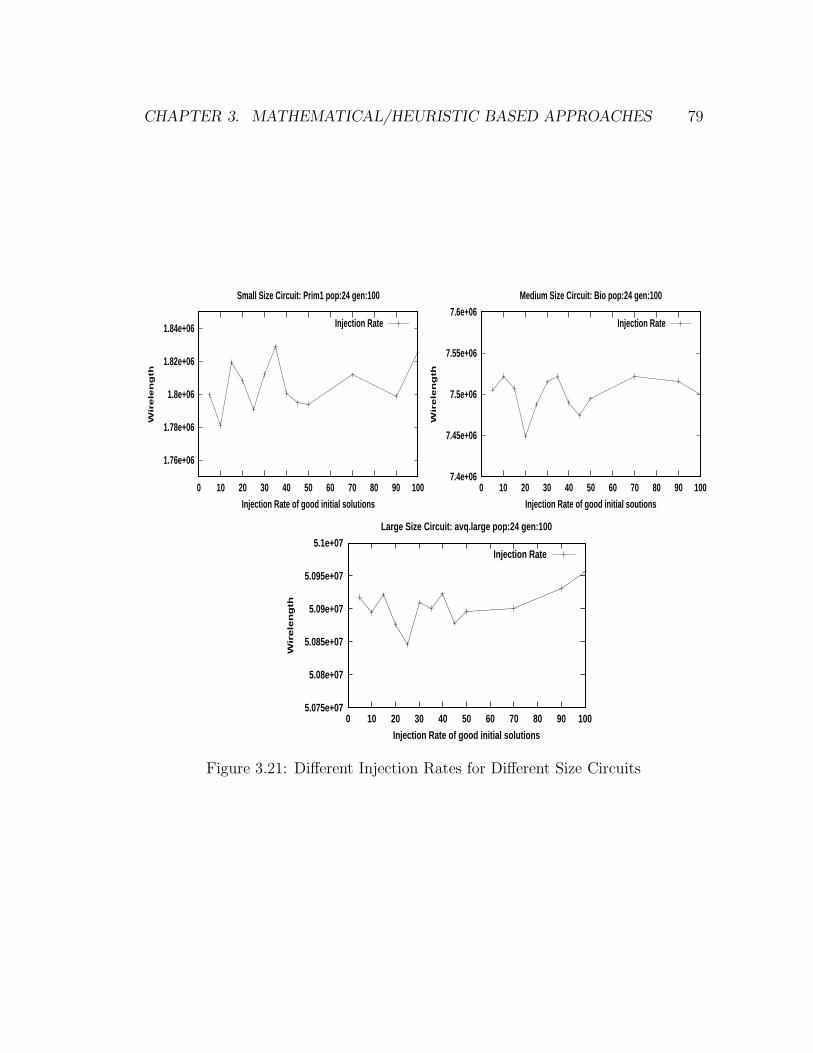
CHAPTER 3. MATHEMATICAL/HEURISTIC BASED APPROACHES 79
1.76e+06
1.78e+06
1.8e+06
1.82e+06
1.84e+06
0 10 20 30 40 50 60 70 80 90 100
Wir
ele
ng
th
Injection Rate of good initial solutions
Small Size Circuit: Prim1 pop:24 gen:100
Injection Rate
7.4e+06
7.45e+06
7.5e+06
7.55e+06
7.6e+06
0 10 20 30 40 50 60 70 80 90 100
Wir
ele
ng
th
Injection Rate of good initial soutions
Medium Size Circuit: Bio pop:24 gen:100
Injection Rate
5.075e+07
5.08e+07
5.085e+07
5.09e+07
5.095e+07
5.1e+07
0 10 20 30 40 50 60 70 80 90 100
Wir
ele
ng
th
Injection Rate of good initial solutions
Large Size Circuit: avq.large pop:24 gen:100
Injection Rate
Figure 3.21: Different Injection Rates for Different Size Circuits
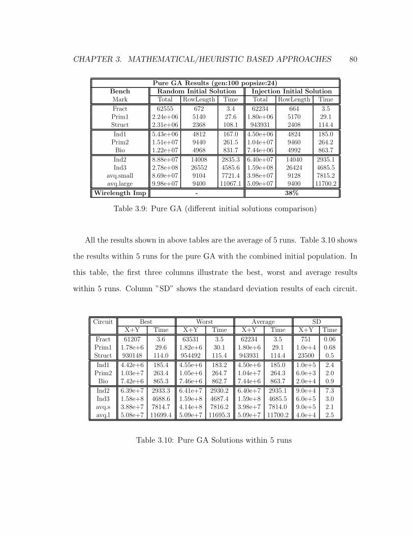
CHAPTER 3. MATHEMATICAL/HEURISTIC BASED APPROACHES 80
Pure GA Results (gen:100 popsize:24)Bench Random Initial Solution Injection Initial SolutionMark Total RowLength Time Total RowLength Time
Fract 62555 672 3.4 62234 664 3.5Prim1 2.24e+06 5140 27.6 1.80e+06 5170 29.1Struct 2.31e+06 2368 108.1 943931 2408 114.4
Ind1 5.43e+06 4812 167.0 4.50e+06 4824 185.0Prim2 1.51e+07 9440 261.5 1.04e+07 9460 264.2Bio 1.22e+07 4968 831.7 7.44e+06 4992 863.7
Ind2 8.88e+07 14008 2835.3 6.40e+07 14040 2935.1Ind3 2.78e+08 26552 4585.6 1.59e+08 26424 4685.5
avq.small 8.69e+07 9104 7721.4 3.98e+07 9128 7815.2avq.large 9.98e+07 9400 11067.1 5.09e+07 9400 11700.2
Wirelength Imp - 38%
Table 3.9: Pure GA (different initial solutions comparison)
All the results shown in above tables are the average of 5 runs. Table 3.10 shows
the results within 5 runs for the pure GA with the combined initial population. In
this table, the first three columns illustrate the best, worst and average results
within 5 runs. Column ”SD” shows the standard deviation results of each circuit.
Circuit Best Worst Average SDX+Y Time X+Y Time X+Y Time X+Y Time
Fract 61207 3.6 63531 3.5 62234 3.5 751 0.06Prim1 1.78e+6 29.6 1.82e+6 30.1 1.80e+6 29.1 1.0e+4 0.68Struct 930148 114.0 954492 115.4 943931 114.4 23500 0.5
Ind1 4.42e+6 185.4 4.55e+6 183.2 4.50e+6 185.0 1.0e+5 2.4Prim2 1.03e+7 263.4 1.05e+6 264.7 1.04e+7 264.3 6.0e+3 2.0Bio 7.42e+6 865.3 7.46e+6 862.7 7.44e+6 863.7 2.0e+4 0.9
Ind2 6.39e+7 2933.3 6.41e+7 2930.2 6.40e+7 2935.1 9.0e+4 7.3Ind3 1.58e+8 4688.6 1.59e+8 4687.4 1.59e+8 4685.5 6.0e+5 3.0avq.s 3.88e+7 7814.7 4.14e+8 7816.2 3.98e+7 7814.0 9.0e+5 2.1avq.l 5.08e+7 11699.4 5.09e+7 11695.3 5.09e+7 11700.2 4.0e+4 2.5
Table 3.10: Pure GA Solutions within 5 runs

CHAPTER 3. MATHEMATICAL/HEURISTIC BASED APPROACHES 81
3.5.3.2 Memetic Algorithm Results
As indicated in section 3.5.2, a pure GA is not well suited for exploring the solu-
tion space. To improve the fine local tuning capability of a Genetic Algorithm, a
Memetic (hybrid) Genetic Algorithm was proposed in this thesis. Table 3.11 com-
pares the performance of a pure Genetic Algorithm with three different Memetic
Algorithms. The pure GA is combined with Tile-based local search in three differ-
ent ways, referred to here as (i)“GA-ME-1” (before the crossover) (ii)“GA-ME-2”
(after the crossover) (iii)“GA-ME-3” (before and after the crossover). Cluster-Seed
based results are injected into both pure GA and Memetic algorithms as part of
the initial population. From the last row of the table, it can be seen that the total
wire-length improvement achieved by the different Memetic algorithms is 44%, 43%
and 47% respectively. Obviously, integrating GA with local search in the first two
Memetic methods reduce the amount of wire-length and CPU time on average by
44% and 17% respectively. The last method “GA-ME-3” enhances the wire-length
quality at the expense of an increase in CPU time on average by 40%.
3.5.3.3 Hierarchical Approach Results
It is evident from the previous section that Memetic Algorithms produce much
better results than pure Genetic Algorithms. Yet the computation time of GA (even
for Memetic Algorithm) is large. One technique used to deal with this problem is
to utilize a multi-level hierarchical approach.
Table 3.12 illustrates the effects of different clustering depths on solution quality
and computation time of the pure GA. For the results in the second, third and forth

CHAPTER 3. MATHEMATICAL/HEURISTIC BASED APPROACHES 82
Performance of Memetic AlgorithmsBench Pure GA GA-ME-1 GA-ME-2 GA-ME-3Mark X+Y Time X+Y Time X+Y Time X+Y Time
Fract 62234 3.5 34997 15.1 35942 15.4 34953 31.1Prim1 1.80e+06 29.6 995713 233.2 1.02e+06 219.6 1.00e+06 467.8Struct 943931 114.4 504720 288.8 490276 251.0 460289 600.7
Ind1 4.50e+06 185.0 2.21e+06 926.9 2.07e+06 876.6 2.14e+06 1806.0Prim2 1.04e+07 264.2 5.48e+06 741.3 5.44e+06 685.8 5.47e+06 1451.5Bio 7.44e+06 863.7 3.98e+06 1256.8 4.01e+06 1240.0 3.12e+06 2492.7
Ind2 6.40e+07 2935.1 2.97e+07 3185.7 3.08e+07 3055.8 2.78e+07 6522.6Ind3 1.59e+08 4685.5 9.92e+07 5716.4 1.01e+08 5313.4 9.31e+07 11405.4
avq.small 3.98e+07 78152. 2.10e+07 5278.9 2.09e+07 5033.9 2.02e+07 10130.6avq.large 5.09e+07 11700.2 2.34e+07 6422.6 2.35e+07 6065 2.27e+07 12387.4
Improve 0% 0 % 44% 15% 43% 20% 47% -39%
Table 3.11: Results Comparison of Memetic Algorithms
columns, the clustering depth is 1, 2, and 3 respectively. The pure GA with partially
injected good initial solutions was invoked at the top clustering level only. There
is no further improvement performed on the circuit at top level and succeeding
flattening stages. The results clearly show that, as the clustering technique is
integrated within the pure Genetic Algorithm, the run time is largely reduced,
especially for clustering level-3 (the run time is decreased by 85%). However, the
total wirelength is also increased by 32%.
The quality deterioration is partially due to the approximations made when
the circuit is clustered and local improvements performed at the top level. It
is these approximations that lead to significant quality deterioration during de-
clustering, when these approximations made at the top hierarchical level “trickle-
down” through each de-clustering step. Therefore, localized improvers should be
used to minimize this deterioration as it is introduced at each de-clustering phase.
Since most improvement work is done at the top level, an improver that can find

CHAPTER 3. MATHEMATICAL/HEURISTIC BASED APPROACHES 83
Circuit Flat GA Clust-level-1 Clust-level-2 Clust-level-3X+Y Time X+Y Time X+Y Time X+Y Time
Fract 62234 3.5 80124 2.0 78864 1.7 54548 1.5Struct 943931 114.4 2.99e+06 30.3 2.41e+06 20.6 1.39e+06 14.3Prim1 1.80e+06 29.6 3.15e+06 20.4 2.83e+06 14.8 2.18e+06 9.4
Ind1 4.50e+06 185.0 6.46e+06 78.2 5.61e+06 67.6 3.81e+06 47.6Prim2 1.04e+07 264.3 1.94e+07 137.2 1.64e+07 100.7 1.21e+07 54.2Bio 7.44e+06 863.7 1.63e+07 598.7 1.25e+07 367.3 6.15e+06 64.6
Ind2 6.39e+07 2933.3 1.26e+08 1512.5 1.16e+08 1000.5 7.42e+07 642.5Ind3 1.59e+08 4685.5 4.30e+08 2303.3 3.85e+08 1216.3 2.86e+08 816.3
avq.small 3.98e+07 7813.0 8.44e+07 3232.2 7.45e+07 1693.1 4.51e+07 1203.2avq.large 5.09e+07 11700.2 1.33e+08 7323.4 1.13e+08 3416.4 6.13e+07 1606.4Total 33.46+07 28478 73.7e+07 12006 65.38+07 6205 49.17+07 4460
Improve 0% 0% -55% 58% -49% 78% -32% 85%
Table 3.12: Placement Results at Different Clustering Levels
a local minimum efficiently is needed. In this thesis, a Tile-based local search is
used as the local improver. Table 3.13 shows the effectiveness of the Tile-based
local search used during de-clustering. All the results shown in second and third
columns were attained by applying three levels of clustering. The second column
“Clust-GA-No-Imp” lists the placement solutions without further improvement at
each clustering level, while the third column “Clust-GA-Imp” shows the results
with Tile-based improver at each clustering level. Obviously by performing the
local improver during de-clustering, the hierarchical approach achieves almost the
same quality of solution as the flat approach, with 3 times speed up.
Table 3.14 shows the results obtained by a Genetic Algorithm (Pure GA), a GA
with clustering technique (GA-GC), a Memetic Algorithm with simple Tile-based
local search (GA-Tile) and a GA based on clustering technique with a Tile-based
local search embedded (GA-GC-Tile). It is clear from this table that the algorithm
based on both clustering and simple local search produces high quality solutions.

CHAPTER 3. MATHEMATICAL/HEURISTIC BASED APPROACHES 84
Circuit Flat Pure GA Clust-GA-No-Imp Clust-GA-ImpX+Y Time X+Y Time X+Y Time
Fract 62234 3.5 54548 1.5 39482 4.9Struct 943931 114.4 1.39e+06 14.3 736966 62.2Prim1 1.80e+06 29.1 2.81e+06 9.4 2.09e+06 32.3
Ind1 4.50e+06 185.0 3.87e+06 47.6 2.22e+06 166.6Prim2 1.04e+07 264.2 1.21e+07 54.2 7.76e+06 158.2Bio 7.44e+06 863.7 6.15e+06 64.6 4.43e+06 275.4
Ind2 6.40e+07 2935.3 7.42e+07 642.5 5.42e+07 1185.5Ind3 1.59e+08 4685.6 2.86e+08 861.3 1.81e+08 1374.6
avq.small 3.98e+07 7815.7 4.51e+07 1203.0 3.53e+07 1219.4avq.large 5.09e+07 11700.2 6.13e+07 1606.4 4.30e+07 2144.6Total 33.46+07 28478 49.17e+07 4460 32.07e+07 9271
Improve 0% 0% -32% 85% 4% 67%
Table 3.13: Placement Results with Tile-based Improver
Performance of Hierarchical ApproachBench Pure GA GA-GC GA-Tile GA-GC-TileMark X+Y Time X+Y Time X+Y Time X+Y Time
Fract 62234 3.5 39482 4.9 34953 31.1 34627 22.9Prim1 1.80e+06 29.6 2.09e+06 32.3 1.00e+06 467.8 964815 438.2Struct 943931 114.4 736966 62.3 460289 600.7 464454 544.8
Ind1 4.50e+06 185.0 2.22e+06 166.6 2.14e+06 1806.0 1.97e+06 1318.4Prim2 1.04e+07 264.2 7.76e+06 158.5 5.47e+06 1451.5 5.31e+06 1286.9Bio 7.44e+06 863.7 4.43e+06 275.4 3.12e+06 2492.7 2.77e+06 2157.9
Ind2 6.40e+07 2935.1 5.42e+07 1185.5 2.78e+07 6522.6 3.10e+07 5420.7Ind3 1.59e+08 4685.5 1.81e+08 1374.3 9.31e+07 11405.4 8.06e+07 7521.4
avq.small 3.98e+07 7815.7 3.53e+07 1219.4 2.02e+07 10130.6 1.35e+07 9711.6avq.large 5.09e+07 11700.2 4.30e+07 2144.6 2.27e+07 12387.4 1.60e+07 11060.4
Total 33.46+07 28478 32.07e+07 9271 17.67+07 47294 15.26+07 39478
Improve 0% 0% 4% 67% 47% -39% 54% -27%
Table 3.14: Results Comparison of Hierarchical Approach

CHAPTER 3. MATHEMATICAL/HEURISTIC BASED APPROACHES 85
The results shown in the first two columns indicate that by combining the clustering
technique with GA the computation time involved in producing the same quality
of solutions as the flat pure Genetic Algorithm was largely reduced by 67%. The
amount of improvement in total estimated wire-length achieved using Memetic
algorithm (GA-Tile) is 47% but the computation time involved using a Memetic
algorithm also increases largely. A clustering Memetic Algorithm (GA-GC-Tile)
improves the solution quality by 54% and the computation time is less than that
of the flat Memetic Algorithm (GA-Tile).
The flat and hierarchical Memetic approaches are also compared with ARP
algorithm, as shown in Tables 3.15 and 3.16. For the small size circuits, the results
produced by the Memetic approaches are close to or even better than those of
ARP methods. For the medium and large size circuits, both flat and hierarchical
Memetic approaches can not produce competitive results. The computation time of
Memetic algorithms are much higher than ARP methods. The results comparison
indicates that although Memetic algorithms are a powerful algorithmic paradigm
for evolutionary computing, the Memetic algorithm presented in this thesis still
need to be improved for larger size circuits.
3.6 Summary
In this Chapter, several constructive techniques for circuit placement were intro-
duced and compared. Both flat and hierarchical approaches were used to find the
effectiveness of these approaches. Most solutions obtained by the ARP algorithm
and Partitioning based algorithm are superior to those obtained by the ClusterSeed

CHAPTER 3. MATHEMATICAL/HEURISTIC BASED APPROACHES 86
Performance Comparison (Flat Level)Bench ARP Memetic GAMark X+Y Time X+Y Time
Fract 33928 2.0 34953 31.1Prim1 840792 27.4 1.00e+06 467.8Struct 447726 36.8 460289 600.7
Avg 4.41e+05 22.0 4.98e+05 366.5
Ind1 1.67e+06 138.8 2.14e+06 1806.0Prim2 4.20e+06 118.5 5.47e+06 1451.5Bio 2.31e+06 172.4 3.12e+06 2492.7
Avg 2.73e+06 143.2 3.58e+06 1916.3
Ind2 2.01e+07 729.6 2.78e+07 6522.6Ind3 5.09e+07 857.3 9.31e+07 11405.4
avq.small 9.65e+06 1219.4 2.02e+07 10130.6avq.large 1.10e+07 2144.6 2.27e+07 12387.4
Avg 3.06e+07 1237.2 4.10e+07 10111.0
Table 3.15: Results Comparison of Different Approaches (flat level)
Performance Comparison (clustering level-3)Bench ARP Memetic GAMark X+Y Time X+Y Time
Fract 38492 3.4 34627 22.9Prim1 1.36e+06 40.8 964815 438.2Struct 491072 48.0 464454 544.8
Avg 6.30e+05 30.7 4.88e+05 335.2
Ind1 1.69e+06 156.4 1.97e+06 1318.4Prim2 4.45e+06 154.0 5.31e+06 1286.9Bio 2.63e+06 253.5 2.77e+06 2157.9
Avg 2.92e+06 187.6 3.35e+07 1587.1
Ind2 2.16e+07 802.2 3.10e+07 5420.7Ind3 5.04e+07 894.3 8.06e+07 7521.4
avq.small 7.12e+06 1052.8 1.35e+07 9711.6avq.large 7.85e+06 1119.3 1.60e+07 11060.4
Avg 2.18e+07 969.0 3.52e+07 8428.0
Table 3.16: Results Comparison of Different Approaches (Clustering Level-3)

CHAPTER 3. MATHEMATICAL/HEURISTIC BASED APPROACHES 87
based algorithm and Random placement. By using the multi-level clustering tech-
nique, the computation time of the ARP algorithm which produces the best results
was reduced significantly by 85%. By performing the iterative improvement on the
initial placement solution at clustering level-3, the quality of the results produced
by Partitioning based placement was close to those produced by the ARP algorithm
in less time.
An evolutionary based algorithm (GA) was developed to explore the solution
space more effectively. By injecting the high quality solutions into the initial popu-
lation, the convergence rate of the pure GA was dramatically increased. In order to
improve the final local tuning capability of a pure GA, a Memetic Algorithm that
combines global and local search (by using GA to perform exploration while the
local search performs exploitation) was presented. It was shown that this hybrid
search technique is very effective. While the placement quality is improved by the
Memetic algorithm, the computation time is still high, especially for large circuits.
To deal with this problem, a clustering technique was incorporated in the pure
Genetic Algorithm and Memetic Algorithm. As can be seen from the experimen-
tal results, the hierarchical approaches produced the same or even better solutions
than the flat approaches with less computation time.
In Chapter 4 another objective of the placement problem (congestion minimiza-
tion) is introduced and a post processing technique is incorporated into a traditional
wirelength-driven placement algorithm (ARP) to reduce the congestion.

Chapter 4
Congestion-driven Placement
4.1 Introduction
Physical design is a complex process, therefore, it is usually broken down into
various sub-steps in order to handle the complexity of the problem. Inherent in
decomposing any problem is the fact that every time a given subproblem is solved,
some information about relationships/dependencies with other subproblems is lost.
This chapter tackles this problem by simultaneously considering the routing prob-
lem within the placement phase. The merits of performing both processes jointly
seems unquestionable, especially for circuits with millions of transistors. Traditional
placement algorithms mainly focus on minimizing total estimated wire length to
obtain better routability and smaller layout area [AD85, Sun93, Klei91]. However,
a placement with less total wire length but highly congested regions often leads
to routing detours around the region, in turn resulting in a larger routed wire
length [Yang01b]. Congested areas can also downgrade the performance of global
88

CHAPTER 4. CONGESTION-DRIVEN PLACEMENT 89
routers, and in the worst case, create an unroutable placement in the fix-die regime
[Cald00]. If congested regions are detected, a new placement of cells in these (and
maybe other) regions is necessary. This can lead to several iterations of the place-
ment phase to get a routable placement. For small designs, such iterations may
be acceptable, but with the growing complexity of chips (i.e. state-of-art chips
have tens of millions of movable objects [Bren02]) routing problems cannot be han-
dled in reasonable time. Therefore, congestion is becoming an important objective.
Although the congestion problem is widely addressed in routing algorithms, the
optimization performance is constrained because the cells are already fixed at the
routing stage. Hence, it is of value to consider routability in the placement stage
where the effort on congestion reduction would be more effective.
In this chapter, the previous work on congestion reduction is introduced in
section 4.2. In section 4.3, a congestion reduction technique is presented and incor-
porated into a placement approach. One of the main contributions of this thesis is
to investigate the effectiveness of flat and hierarchical approaches for congestion-
driven placement. The corresponding results are shown in section 4.4.
4.2 Congestion Based Technique
4.2.1 Congestion Cost
In general, the congestion problem can be modeled as the summation of a linear
[Wang99] or quadratic [Chen94] function of difference between routing demand and
routing supply based on the global bin concept. First, a given chip is partitioned
into a set of rectangular regions, called global bins. The boundaries of global bins

CHAPTER 4. CONGESTION-DRIVEN PLACEMENT 90
are called global bin edges. Figure 4.1 shows an example with 16 global bins. For
Global Edges
Global Bins
Figure 4.1: Layout of a Circuit and Global Bins
each global bin edge e, the routing demand de is the number of wires that cross this
boundary; the routing supply se is the number of wires that are allowed to cross
boundary. The difference between routing demand and supply is formally described
as :
overflowe =
de − se if de > se;
0 if de ≤ se.
The total overflow of a placement is defined as the summation of the overflow
for all global edges 1. Thus, a placement with less total overflow is less congested.
The supply of routing resources can be computed from the technology parameters
of the design. The demand for routing resources depends on the placement and
routing solutions. However, fully accurate routing demand is not available until
after detailed routing. Therefore, estimation algorithms are required for congestion
1The amount of total overflow reflects the amount of total shortage of routing resources in theplacement.

CHAPTER 4. CONGESTION-DRIVEN PLACEMENT 91
analysis during an earlier phases of the design. Two new congestion estimation
models: a Rent’s rule based model and a probabilistic model were proposed in
[Yang01b, Lou01], respectively.
4.2.2 Previous Work
In the last couple of years several new approaches have been developed in order to
take into consideration congestion during the placement phase. These congestion
reduction techniques can be classified into two types:
• Integrating congestion into a traditional wirelength-based placement
algorithm [Chen94, Meix90, Para98, Hou01, Bren02].
• Performing a post placement processing step to reduce the congestion
[Wang99, Wang00b, Wang00c, Yang01a, Wang00a].
In the rest of this section, a brief survey of the existing major methods of
congestion reduction is provided.
4.2.2.1 Integrated Approach
In [Meix90], a congestion-driven placement based on a multi-partitioning technique
was introduced. It uses pre-determined Stenier trees to model the net topologies,
which accounts for wiring congestion into account. The objective of the algorithm
is to minimize the total number of track segments for the interconnections of all
nets. Usually, the multi-partitioning process is subject to a balance criterion which
admits only those partitions whose partitions satisfy user specified area constraints.
In the proposed approach, the authors not only consider the total amount of cell

CHAPTER 4. CONGESTION-DRIVEN PLACEMENT 92
area Aci of each partition, but also account for the wiring area necessary for the
interconnections. One way to accomplish this is to translate the track demand of
each partition Pi into an equivalent wiring area Awi by examining the net topologies
for all nets.
During the partitioning process, the objective can be evaluated using the topology-
matrix T and the concept of a distribution vector of a net (shown in Table 4.1).
Partitions Nets1 ... n ... N
partition 1 t11 ... t1n ... t1N
. . .partition 2 ti1 ... tin ... tiN
. . .partition L tL1 ... tLn ... tLN
Table 4.1: Topology Matrix T
In this table, tin is defined as the number of cells of net n assigned to partition
i. Each row corresponds to one partition, and each column describes the cell dis-
tribution of a net. A distribution vector d is used to represent the cell distribution
of each net in the partition i. For example, the distribution vector d for net n is
defined as follows:
d[i] =
1 if tin > 0;
0 otherwise.
The authors define the nets with∑L
i=0 d[i] ≥ 2 as global nets, and nets with
∑Li=0 d[i] = 1 as local nets. For global nets, the interconnections are implemented
as Steiner trees on the partitioning-graph. During the partitioning process, there
may be 2L different distribution vector d[i] occurring, where L is the number of
partitions. In order to accelerate the algorithm, the Stenier trees are calculated
CHAPTER 4. CONGESTION-DRIVEN PLACEMENT 93
only once in a preprocessing step. Once the net topology of each net is determined
by the distribution vector, the wiring area Awi of partition i can be derived by
examining the net topologies of all nets. For a global net, all edges of the corre-
sponding Steiner trees are considered. For each local net, the wiring area is assumed
as 0.5 times the half perimeter of the corresponding region. The intra-cell wiring
of all cells assigned to partition i is also considered. The total area of partition i is
defined as:
Ai = Awi + Aci
where Aci is the total cells area of partition i, and Awi is the total wiring area for the
interconnections. An upper and lower bound of the total area is then introduced for
each partition. Keeping the total area of every partition within the upper and lower
bounds gives rise to a better distribution of cells and wiring over the placement area
because a high track demand for a partition leads to a low cell population in a par-
tition and vice versa. A partitioning is said to be accepted if the balance criterion is
satisfied. After each cell-based moving, the corresponding columns of the topology-
matrix, the Steiner trees, and the wiring areas of affected partitions need to be
updated. The experimental results have shown that the number of track segments
is significantly reduced by 16% on average compared to recursive min-cut bisection
and global optimization methods. However, the number of partitions allowed in
this approach has to be restricted because the number of distribution vectors grows
exponentially with the number of partitions and the proposed algorithm is only
tested on five relatively small sea-of-gates designs. Besides, the amount of change
made to the wirelength and computation time used are not mentioned in [Meix90].
In [Chen94], a routability model based on the supply versus demand analysis

CHAPTER 4. CONGESTION-DRIVEN PLACEMENT 94
of routing resource over an array of regions on a chip was proposed. The analysis
results produced by this routability model is then transformed into a component
of the cost function of simulated annealing. Initially, every region contains the
same amount of routing supply. Existing wiring of power, clocking nets, regular
cells, and mega cells are considered to be an obstacle to routing. The routing
resource supply decreases when any of these is found in a region. Based on the
equations presented in [Chen94], the real routing supply of each region can be easily
obtained without expensive calculations during the pre-processing. The routing
resource demand model used is based on net bounding box. A special technique
used to handle nets overlapping with mega cells (a cell that is much larger than
any regular cell and has a subset of metal layers fully blocked at current design
level) is also introduced. While the reduction of the congestion clearly highlights
the advantages of the model, the proposed approach discards the extensive research
work on wirelength minimization, and it significantly degrades placement speed.
P.N. Parakh [Para98] proposed a method that drives quadratic placement to
relieve congestion while simultaneously solving for minimal wire length. In this
paper, a placement produced by the quadratic placer is iteratively partitioned into
regions, and placed with new center of gravity constraints. Before each successive
placement, internal route estimation and region-based global route are performed
on each region to estimate the supply-demand ratios. The interplay between rout-
ing analysis and quadratic placement is accomplished by using a growth matrix to
permit global treatment of congestion. The use of growth matrix causes cell posi-
tions to reflect supply-demand ratios of different regions. Resource limited regions
are expanded (or reduced) to account for the wiring demand imposed on them. The

CHAPTER 4. CONGESTION-DRIVEN PLACEMENT 95
horizontal ratio is used to stretch the region in the Y direction, while the vertical ra-
tio stretches the region in the X direction. The growth factors disperse cells within
a region and influence other cell positions while permitting the solver to minimize
the objective function. For example, in Figure 4.2(a) a region is deemed vertically
congested according to the horizontal supply-demand ratio. Therefore a vertical
expansion is then performed. After expansion, some internal horizontal nets could
become vertical, thus relieving congestion (as shown in Figure 4.2(b)). If the region
is shrunk horizontal based on the vertical ratio, during the next iteration more nets
from the previous iteration could become vertical, further relieving congestion (as
shown in Figure 4.2(c)). In addition, congestion induced by incorrect pin order-
ing is relieved by relaxing the pin constraints to a single dimension such that the
routing congestion is further reduced.
(b) Vertical Expansion (c)Routes Transformation (a) Horizontal Congestion
congested region
Figure 4.2: Example of Region Growth Relieving Congestion
The performance of the proposed algorithm is tested on the ISCAS-89 bench-
marks [ISCA89] and the experimental results shows up to 20% reductions in average
demand-supply excess. The total route length determined by a global router for all
benchmark circuits is increased by 2.3% on average.
A similar congestion-driven placement algorithm based on cell inflation was pro-
posed in [Hou01]. Instead of expanding the congested regions, it expands the cells

CHAPTER 4. CONGESTION-DRIVEN PLACEMENT 96
inside the congested bins such that the congestion is checked and eliminated while
doing the partitioning process. A Star estimation model is adopted to estimate the
routing of each net. For example in Figure 4.3, a five-pin net is first transformed
into a star-model net (shown in Figure 4.3(b)). The route that connects each pin
to the center is estimated. When there are two possible routing paths for a net,
the probabilities that the route go through path A or B are equal. According to
this method, the result of routing estimation is shown in Figure 4.3(c). Finally,
the total number of tracks required of all the global bins that the net has passed
through represents the routing demand of this net.
Pin3
Pin1
Pin2
Pin4
Pin5
(b) Star model
0.5
0.5
0.5
1.5 0.5
1.0
0.5
0.5 0.5
0.50.5
1.0
1.51.0 1.0Pin3
Pin1
Pin2
Pin4
Pin5
(a) Five−pin net (c) Routing estimation of the five−pin net
Figure 4.3: Routing Estimation Model
In the routing estimation and congested bin detecting stage, the real area of the
cell is used. After the congested bins are identified, the cells in the congested bins
are expanded. In next partitioning loop, during which the expanded virtual areas
of cells are used, some cells located in the congested bins will be forced to move to
other bins because of the area-balance rule. As a result, the number of cells located
in the congested bins will decrease. In general, a bin with less cells will have fewer
nets to be passed through and therefore the congestion will be reduced. After the
global placement, a cell based moving is performed to erase the routing congestion

CHAPTER 4. CONGESTION-DRIVEN PLACEMENT 97
more deeply. An example for cell inflation is shown in Figure 4.4. There are four
cells and five nets in the top-left congested bin A and the areas of the four cells
located in bin A are expanded. After next partition loop, due to area balance, cell
C is forced to move to bin B. As a result, there are only three cells and four nets
in bin A. Thus, the routing resource supply increases while the routing demand
decreases, as shown in Figure 4.4(b).
C
C
(b) After cell Inflation(a) Before cell Inflation
bin B
congested bin A congested bin A
bin B
Figure 4.4: Cell Inflation Example
The performance of the proposed approach is tested on a set of sample circuits
from American industry. The experimental results show that the maximum con-
gestion (the number of track shortage in the most congested bin at both x and
y directions) can be cut down by about 30-40%, while the total wirelength in-
creased slightly (there is no detail numerical results of total wirelength increasing
reported). Besides, the run time of the presented approach is doubled compared
with the conventional wirelength-driven partitioning placement approach.
In ISPD’02, U. Brenner [Bren02] and his colleague presented a fast but reliable
method to estimate the congestion in a region at the global placement stage and
incorporated this congestion estimation model into a partitioning based placement
algorithm. The proposed congestion estimator is a simplified probabilistic region
CHAPTER 4. CONGESTION-DRIVEN PLACEMENT 98
global router. Based on this router, in the first placement run, the congested regions
are found and the cells inside these congested regions are inflated. The inflation rate
of each cell is updated according to the congestion estimation of the region that the
cell is currently placed in. Following that, a repartitioning method is performed on
the congested regions to move cells out of regions that are too full (with respect to
the inflated cell size). In this process, only the congested regions that are too full but
have neighboring regions with some free capacity are considered. For each selected
region, a repartitioning subroutine is called to compute a new partitioning positions
for the cells in this region. The new partitioning is accepted if the overcrowding
is reduced. This repartitioning process is performed repeatedly as long as it yields
a reasonable improvement on the wirelength. The presented algorithm is tested
on five benchmark circuits from IBM Microelectronics. Experimental results show
that the usage of the most critical routing edges is reduced by 9.0% on average
and the bounding box netlength is increased by 8.5%. Although the CPU-time for
placement increased by 8.7% the total CPU-time for placement and global routing
is decreased by about 47%.
4.2.2.2 Post-processing Approach
In practice, combining a global router and placer is an effective way to improve
routability, but researchers keep studying other efficient approaches to handle the
increasing design size.
In a recent study [Wang99, Wang00b], the behavior of congestion minimization
in placement was analyzed from both theoretical and experimental perspectives. In
these papers, the authors first pointed out that congestion minimization and wire-

CHAPTER 4. CONGESTION-DRIVEN PLACEMENT 99
length minimization correlate with each other in a global view but conflict each
other in local regions. According to this relationship, they further proposed a two
stage process to reduce the congestion in a layout, where the wirelength driven
global placement (which can also reduce the congestion globally) is performed ini-
tially. A post-processing stage is then used to reduce local congested spots. They
found that the congestion objective function is very ill behaved and therefore, di-
rectly using it will not produce low congestion placement. By incorporating a more
sensitive congestion objective function, called “overflow with look-ahead” into a
Net-centric algorithm at the post-processing stage, the congestion of eight MCNC
standard-cell benchmark circuits was reduced by 36.9% on average. Nevertheless,
this method need to use the same routing model in the placement as the model
used in the final routing stage.
While congestion was reduced significantly by using the technique presented in
[Wang99, Wang00b], the wirelength was also increased by 5-10%. The increase in
wirelength implies that placement is changed. This change may result in viola-
tions to other performance constraints (i.e timing and couplings) which are hard
to achieve. However, since much of performance constraints including timing and
coupling are locally stable, there will be no violations in the constraints as long as
the change in the placement is bounded locally. In [Wang00c], a heuristic method,
named “Multi-Center Congestion Reduction” was proposed for congestion mini-
mization with minimal change in placement. This method also belongs to a post-
processing congestion reduction technique. During the post-processing stage, a
normal distribution is utilized to approximate the actual congestion. The tool then
derives an equation from the normal distribution to estimate the amount of con-

CHAPTER 4. CONGESTION-DRIVEN PLACEMENT 100
gestion on a layout. Each congested spot is then identified by finding a minimum
bounding rectangular region of a set of connected congested bins. Next, the con-
gestion reduction regions are formed by using each congested spot as a center to
expand. The technique is based on a scheme called “flexible expansion scheme”
which can decrease congestion while keeping placement unchanged as much as pos-
sible. Figure 4.5 illustrates the expansion scheme. The current congested region
Expand to right
Expand downward
Expand upward
Expand to left
Current region
New region
Figure 4.5: Example of Region Expansion
is first expanded in four possible ways: up, down, left and right. The routability
of the four newly expanded regions are evaluated and the one with best estimated
routability is picked as the new region. The procedure is repeated until the es-
timated routability of the new region is better than an expected value. If the
routability of the new region is worse than that of the original region or the new
region occupies the whole layout area the technique is invoked again. Finally, a
random greedy method [Wang99] is performed within each expanded congestion
reduction region to relieve the congestion. The experimental results based on the
MCNC standard-cell benchmark circuits show that this algorithm can reduce con-
gestion by 41% (almost by the same amount as in [Wang99]) and increase the

CHAPTER 4. CONGESTION-DRIVEN PLACEMENT 101
wirelength by only 1.8% on average.
Although it is reported in [Wang99, Wang00c, Wang00b] that the post-processing
technique is more efficient than directly minimizing congestion, reducing congestion
after a wirelength placement is a non-trivial problem. Traditionally, some perturba-
tion is performed on an existing placement within a window around the congested
spots [Wang00c, Tsay92]. Local improvement within small windows has limited ef-
fect, whereas expanding search windows may cause interactions between congested
areas, making the optimization results unpredictable. To identify a combination of
expansion scheme for all the congested regions such that the maximum congestion
over the core area is minimized, a novel, integer linear programming based tech-
nique is introduced in [Yang01a]. Based on the bounding box routing estimation
model, one congested region is represented by a minimum bounding rectangular re-
gion of a set of connected congested bins. As indicated in [Yang01a], the congestion
reduction should be performed within a larger region than the congested region be-
cause of the larger solution space. However, a larger expansion area requires longer
running time and increases the likelihood of the overlap regions, which may cause
unexpected new congested regions (as shown in Figure 4.6(a)). Hence, all the con-
gested regions are expanded by using an ILP based double expansion technique
which can find the expansion range for each congested region to avoid the regions
overlap. This is accomplished by assigning two expansion areas (as seen in Figure
4.6(b)) for each region, transforming the expansion area selection problem (choose
the larger expansion area or smaller one) into an integer programming problem,
and then solving the ILP problem. Once the expansion areas are determined, a
local improvement based on cell swapping is performed for each expansion area to

CHAPTER 4. CONGESTION-DRIVEN PLACEMENT 102
reduce the congestion.
Possibly new congested areas
Smaller expansion area
Congested region k
Larger expansion area
Expansion areas
Congested regions
(a) Overlaps between expansion areas (b) Two expansion areas for a congested region
Figure 4.6: Expansion Area Overlaps and Double Expansion Scheme
The experimental circuits are chosen from IBM-PLACE benchmarks [IP] and
the results show that the total overflow is considerably reduced after global routing.
For the best case among all the results, the total overflow of the circuit turns to
zero by congestion reduction. As for the total routed wirelength, almost all the
circuits have shorter wire-lengths after congestion reduction. The decrease in routed
wirelength is about 3.6% on average. In addition, the short amount of running time
illustrates that the method can scale well for large circuits.
In the next section, a congestion-driven placement approach is presented, based
on the post-processing technique. Both flat and hierarchical approaches are used
to find the effectiveness of these approaches.
4.3 Proposed Congestion Reduction Approach
The congestion-driven placement method (as shown in Figure 4.7) proposed in this
thesis is based on incorporating the congestion reduction technique into a hierarchi-
cal placement algorithm. The clustering technique used in the hierarchical place-

CHAPTER 4. CONGESTION-DRIVEN PLACEMENT 103
ment algorithm is same as the technique previously introduced in Chapter 3. In
[Wang99], M. Wang and his colleagues pointed out that a post-processing technique
minimizes congestion effectively because the congestion correlates with wirelength
in a global view. Therefore, the congestion reduction of the proposed congestion-
driven placement method is done in a post-placement-optimization process. To
demonstrate the effectiveness of the proposed congestion reduction method, both
flat and hierarchical approaches are implemented.
Congestion Reduction
Routing Estimation
Congested Region
Expanding
Congestion Reduction
Identification
Congested Region
Module Descriptionand Netlist
Multi−Level Clustering
Wirelength Minimization
Valid Coordinates for
Each Standard−Cell
De−Clustering
Figure 4.7: Congestion-driven Hierarchical Placement
For the flat approach, the placement input of the congestion reduction is pro-
duced by a quadratic placer ARP [Etaw99a] followed by an iterative improvement
approach. The congestion reduction technique (presented in section 4.3.1) is then
performed to further optimize the routability of the placement solution. As for the
hierarchical approach, the algorithm starts by performing the multi-level clustering
technique on the flat layout to group the highly connected cells gradually and thus

CHAPTER 4. CONGESTION-DRIVEN PLACEMENT 104
reduce the complexity of the circuit. At the highest level of the hierarchy, similar to
the flat approach, a good quadratic placement algorithm (ARP) is then performed
followed by an iterative improvement algorithm to optimize the total estimated
wirelength as well as the average congestion. Ultimately, a congestion reduction
technique is invoked to further reduce the local congestion.
4.3.1 Congestion Reduction in Placement
During the congestion reduction stage, the core area of the chip is divided into m×n
grids (also called global bins). For standard-cell designs, n is set to the number of
standard-cell rows; m is set so that the average number of cells per global bin is
less than 3.
The routing supply is determined as follows: initially the placement without
congestion reduction is run and the routing demand is estimated by the bounding
box router (introduced later in this section). Based on the estimated routing de-
mand, the routing capacities of the global bin edges is then set such that certain
amount of overflow is generated.
Routing Estimation
In order to evaluate the congestion during placement, a fast and accurate routing
estimation is required. In the traditional routing estimation models, the minimum
spanning tree model is the most accurate but also the most computationally ex-
pensive. The bounding box model requires the least computation for updating but
generates reasonable estimation. Therefore, in this thesis a bounding box model
used in [Chen94] is considered.

CHAPTER 4. CONGESTION-DRIVEN PLACEMENT 105
(k)ij,hC
C (k)ij,v
b(i,j)
(k)ij,hC
heightbounding box
(k)C
net K
bounding box width
ij,v
Figure 4.8: Bounding Box Routing Estimation Model
As illustrated in Figure 4.8, for each global bin b(i, j) at column i and row
j, the number of horizontal wire crossings on its right edge by net K is repre-
sented as Ckij,h. Similarly, the number of vertical wire crossings on its bottom
edge by net k is represented as Ckij,v. The bounding box of net K is described by
xmin(k), xmax(k), ymin(k), ymax(k). Based on the probability of having a wire
within a global bin covered by the bounding box of net K, the Ckij,h and Ck
ij,v are
computed as follows:
Ckij,h =
q(k)ymax(k)−ymin(k)+1
xmin(k) ≤ i < xmax(k); ymin(k) ≤ j ≤ ymax(k)
0 otherwise
Ckij,v =
q(k)xmax(k)−xmin(k)+1
xmin(k) ≤ i ≤ xmax(k); ymin(k) ≤ j < ymax(k)
0 otherwise
where q(k) is a compensation factor adopted from [Chen94]. The existence of
q(k) is based on the fact that the bounding box wirelength model under-estimates

CHAPTER 4. CONGESTION-DRIVEN PLACEMENT 106
the actual wiring for nets with more than three terminals. Its value depends on the
number of terminals of net k. For 2-terminal or 3-terminal nets, q is 1 and slowly
increases to 2.79 for nets with 50 terminals. This bounding box model approximates
the routing demand efficiently even though it over-estimates routing demand near
the boundaries of a net bounding box.
According to the routing estimation for each net, the total estimated routing
demand for the right and bottom edge of each global bin b(i, j) can be described
as :
Cij,h =N
∑
k=1
Ckij,h
Cij,v =N
∑
k=1
Ckij,v
The number of tracks for vertical and horizontal global bin edges is represented
as Caph and Capv. For bin(i, j), the overflow of the right edge OFij,h is max(Cij,h−
Caph, 0), and the overflow of the bottom edge OFij,v is max(Cij,v − Capv, 0). The
congestion cost function of the design is modeled by a combination of wirelength
(represented by routing demand) and quadratic function of overflow. Based on this
congestion cost function, the solution generated by the congestion reduction tech-
nique is accepted if the over crowding is reduced, even if the wirelength gets worse
slightly. The horizontal congestion CONGcostv and vertical congestion CONGcostv
are:
CONGcosth =m−1∑
i=1
n∑
j=1
(Cij,h +OF 2ij,h)
CONGcostv =m
∑
i=1
n−1∑
j=1
(Cij,v +OF 2ij,v)

CHAPTER 4. CONGESTION-DRIVEN PLACEMENT 107
The total congestion cost CONGCost is the sum of CONGcosth and CONGcostv .
In addition, the total overflow OF of the layout is the sum of overflow over all the
global bin edges:
OF =m−1∑
i=1
n∑
j=1
OFij,h +m
∑
i=1
n−1∑
j=1
OFij,v
Identification of Congested Regions
A global bin is congested if one of its four global edges is congested. The congested
region identification is accomplished by picking a congested global bin as the seed,
checking the neighborhood bins and including the congested bins into the current
congested region. The minimum rectangle that contains these congested bins is
considered as one congested region. A new seed is then picked to form the next
congested region. Since a large congested region may degrade the effect of the
congestion reduction within its range, a maximum number of congested bins in one
congested region is set to prevent forming too large congested regions. Figure 4.9
shows an example of congested region identification.
bin(i,j)
congested
congested region 3
bin(2,3)
congested region 2
(a) neighbood bins (b) total congested regions
congestedbin(0,0)
congested region 1
neighborhoodbins
Figure 4.9: Congested Region Identification
Initially, a set of neighborhood bins (shown in Figure 4.9(a)) around the first

CHAPTER 4. CONGESTION-DRIVEN PLACEMENT 108
selected congested bin b(0, 0) are checked. The congested bins within this neighbor-
hood are then included into this congested region. Once the first congested region
is identified, the algorithm proceeds by picking the next unselected congested bin
(i.e. b(2, 3)) as a new seed and forming next congested region. Finally, the total
three congested regions are found (as shown in Figure 4.9(b)). A pseudo code for
the identification of congested regions is shown in Figure 4.10.
Indentify Congested Regions1. set i=0, j=0;2. FOR each global bin i
IF (bini congested and distinct)Add(bini, regionj);FOR all the neighboring bins of bin iIF (congested and distinct)Add(bini, regionj);
END FOREND IFi++ and j++;END FOR
3. Repeat all the congested regions.4. Stop.
Figure 4.10: Identify the Congested Regions
.
Congested Region Expansion
For a single congested region, the larger the expansion area is, the better the opti-
mization result can be obtained due to the larger solution space [Yang01a]. How-
ever, the expansions of multiple congested regions may lead to region overlaps and
thus generate new congested regions. In this thesis, a congested region is expanded
in four possible ways: up, down, left and right. For the vertical region expansion

CHAPTER 4. CONGESTION-DRIVEN PLACEMENT 109
(up and down), the region has one more row of global bins; For the horizontal
expansion (left and right), the region has one more column of global bins. (an
example is shown in Figure 4.11).
������������������������������
��������������������������������������������������
��������������������������������������������������
�������������������������
�������������������������
�������������������������
������������
����������
������������������������������������������
�������������������������
� � � � � � � � � � � �
�������������������������
������������������������������
�������������������������
�����������������������������������
�������������������������
�����������������������������������
�������������������������
�������������������������
�������������������������
������������������������������������������
�������������������������
original congested region
expansion area
Figure 4.11: Congested Region Expansion
Congestion Reduction
Once the congested regions are determined, a congestion optimization process based
on a greedy cell-swapping is then performed in each region. The main objective
of the heuristic is to reduce the congestion effectively and make as few modifi-
cation (perturbation) as possible. A candidate cell is randomly chosen from an
un-expanded congested region and another is picked from the expansion area. This
pair of selected cells are then swapped and the routing estimation is re-evaluated.
The swap will be accepted if the total congestion cost in the chip area is lower after
swapping, otherwise it is rejected. After each swapping process, the cell overlaps
are removed. The algorithm stops when a certain number of iterations is reached
and the row lengths are adjusted before the termination.

CHAPTER 4. CONGESTION-DRIVEN PLACEMENT 110
4.4 Experimental Results
In this thesis, the quality of the congestion reduction method is measured by the
overflow based on the bounding box routing. Benchmarks used to evaluate the
performance of congestion-driven placement will be based on those presented in
Chapter2.
Since all the results shown in the literature are based on the flat level place-
ment, one of the main objectives of this thesis is to identify if the post-processing
congestion reduction approach can be extended to multi-level clustering.
4.4.1 Flat Level Placement with Congestion Reduction
Circuits Cells Nets Grids #c/bin V/H Cap
Fract 125 147 6x9 2.3 6/6Prim1 752 904 16x21 2.2 11/10Struct 1888 1920 21x32 2.8 8/7
Ind1 2271 2478 15x54 2.8 19/7Prim2 2907 3029 28x49 2.1 16/13Bio 6417 5742 46x60 2.3 11/10
Ind2 12142 13419 72x76 2.2 17/20Ind3 15059 21940 54x111 2.5 27/20
avq.small 21854 22124 80x114 2.4 12/10avq.large 23114 25384 86x120 2.2 12/10
Table 4.2: Tested Circuit Statistics
This section shows the performance of the congestion-driven placement at the
flat level. Table 4.2 shows the statistic information for all the test circuits. The
third column “Grids” shows the number of rows and columns of global bins for
each circuit. The fourth column “#c/bin” shows the average number of cells in each

CHAPTER 4. CONGESTION-DRIVEN PLACEMENT 111
global bin. The last column of this table gives the vertical/horizontal capacities used
in the bounding box routing. For each circuit, the vertical/horizontal capacities
are intentionally adjusted so that a layout with certain amount of overflow can be
achieved.
Table 4.3 illustrates the effect of congestion reduction as a post-processing after
a high-quality wirelength-driven placement (ARP+Tile). The first three columns
of this table present the overflow, total wirelength and running time of the place-
ment without congestion reduction, while the remaining columns present the same
information of the placement with congestion reduction. The percentage of over-
flow and wirelength improvement produced by congestion reduction method are
also shown. For different size of circuits, the average improvement on the overflow
and wirelength are shown in row “Ave-Imp”. The last row “T-Imp” shows the
overall improvement on the overflow and wirelength. As can be seen, after con-
gestion reduction the total overflow of most circuits are reduced largely by 51%
on average. As of total bounding box wirelength, all the circuits have a longer
wirelength after congestion reduction. The wirelength increasing rate is about 3%
on average. This indicates that the high quality placement solution generated by
the wirelength-driven placer (ARP+Tile) is degraded slightly due to the reduc-
tion of overflow. Figure 4.12 summarizes the improvement on the congestion and
wirelength for medium and large size circuits.
Finally, the computation time of the congestion-driven placement is increased
largely compared with the wirelength-driven placement. This fact suggests that a
more efficient congestion reduction method is needed when using the post processing
technique to reduce the congestion.

CHAPTER 4. CONGESTION-DRIVEN PLACEMENT 112
Congestion Estimation After ARP+Tile Placement (flat level)
Bench Without Congestion Reduction With Congestion ReductionMarks OF Wire Time OF Imp% Wire Imp% Time
Fract 10.43 33928 1.8 3.4 66.04% 36534 -8% 2.0Prim1 6.63 840792 27.3 2.02 69.50% 862097 -2.5% 28.1Struct 21.10 447726 37.1 13.06 38.08% 457590 -2.2% 41.8
Ave-Imp - - 58% - -4.23% -9%Ind1 58.07 1.66+6 137.1 18.80 67.62% 1.68+6 -1.2% 148.9
Prim2 224.48 4.20+6 116.2 162.86 27.45% 4.28+6 -1.9% 149.9Bio 105.73 2.31+6 266.2 58.68 44.50% 2.34+6 -1.3% 427.8
Ave-Imp - - 46% - -1.47% -40%Ind2 196.18 2.01+7 720.4 104.06 46.96% 2.04+7 -1.5% 1601.4Ind3 4733.54 5.09+7 900.1 3300.16 30.28% 5.33+7 -4.7% 2001.3
avq.small 446.08 9.65+6 1350.2 187.60 57.94% 9.77+6 -1.2% 3948.4avq.large 322.92 1.10+7 1464.6 138.52 57.10% 1.12+7 -1.8% 3248.9Ave-Imp - - 48.07% - -2.3% -144%T-Imp - - 51% - -3% -64%
Table 4.3: Congestion Reduction After ARP+Tile Placement
0 100 200 300 400 500
Ind1
Prim2
Bio
Ind2
Avq.s
Avq.l
Congestion Reduction after ARP+Tile Placement
Total Overflow
Diff
eren
t Circ
uits
with congestionwithout congestion
0 5 10 15 20 25
Ind1
Prim2
Bio
Ind2
Avq.s
Avq.l
Congestion Reduction after ARP+Tile Placement
Total Wirelength
Diff
eren
t Circ
uits
with congestion without congestion
Figure 4.12: Congestion Reduction After ARP+Tile Placement

CHAPTER 4. CONGESTION-DRIVEN PLACEMENT 113
Table 4.4 lists the distribution of congested regions in 4 quadrants of each bench
mark. Columns “L-B”,“L-T”,“R-B”and “R-T” show the number of congested re-
gions in left-bottom, left-top, right-bottom and right-top regions. The last column
“cong reg Imp” illustrates the improvement on the number of congested regions
respectively. Comparing this table with Table 4.3, we can see that the congested
regions for almost all the test circuits are decreased after performing congestion re-
duction. For circuit Prim2 and Ind3, there is an increase in the number of congested
regions but the total overflow of these two circuits is decreased. This indicates that
although the congested regions of these circuits are increased the average overflow
of each congested region is decreased and therefore the total overflow is decreased.
Bench Before Congestion Reduction After Congestion Reduction congMarks Total Reg Distribution Total Reg Distribution Reg
Regions L-B L-T R-B R-T Regions L-B L-T R-B R-T ImpFract 3 1 1 0 1 3 1 1 0 1 0%Prim1 3 1 1 1 0 2 2 0 0 0 33%Struct 17 1 2 7 7 14 1 2 5 6 18%
Ind1 25 9 6 5 5 21 9 5 2 5 16%Prim2 37 16 13 0 8 38 16 15 1 6 -3%Bio 57 4 18 0 35 41 4 16 0 21 28%
Ind2 78 5 0 10 63 70 6 0 8 56 10%Ind3 276 85 85 79 27 296 101 90 86 19 -7%
avq.small 200 53 14 89 44 145 39 7 73 26 28%avq.large 129 46 17 50 16 108 45 13 41 9 16%
Table 4.4: Distribution of Congested Regions After ARP+Tile Placement
Table 4.5 is similar to table 4.3, except that the input of the congestion reduction
is not a high quality placement but a pure ARP placement. Comparing this table
with Table 4.3, it can be seen that the initial overflow (i.e. without congestion
reduction) of the high quality placement (ARP+Tile) is much less than that of
a lower quality wirelength-driven placement (ARP). This clearly indicates that a

CHAPTER 4. CONGESTION-DRIVEN PLACEMENT 114
Congestion Estimation After ARP Placement (flat level)
Bench Without Congestion Reduction With Congestion ReductionMarks OF Wire Time OF Imp% Wire Imp% Time
Fract 14.69 45211 0.8 8.6 45.49% 45070.5 0.3% 1.0Prim1 105.78 1.13+6 18.3 34.94 66.76% 1.13+6 0% 29.1Struct 673.21 706165 16.4 297.25 55.84% 680721 3.6% 23.9
Ave-Imp - - 56.03% - 1.3% -Ind1 1338.25 2.15+6 89.1 555.04 58.46% 2.16+6 -0.4% 96.1
Prim2 1010.17 5.88+6 104.2 500.65 50.54% 5.89+6 -0.2% 121.2Bio 679.61 3.06+6 151.6 653.06 77.66% 2.97+6 3% 359.2
Ave-Imp - - 62.00% - 0.8% -Ind2 3871.33 2.71+7 790.4 1244.43 67.86% 2.63+7 3% 2047.4Ind3 11259.82 6.90+7 1159 4522.86 59.31% 6.90+7 0% 4071,5
avq.small 902.96 1.36+7 1827 181.38 79.90% 1.31+7 3.7% 2973.6avq.large 801.00 1.64+7 2256 162.17 79.76% 1.54+7 6% 3085.4Ave-Imp - - 71.61% - 3.1% -
Table 4.5: Congestion Reduction After ARP Placment
good wirelength-driven placer can optimize the wirelength as well as the average
congestion at the same time. Hence, it is reasonable to say that a two stage process
for congestion reduction is very useful. In the first stage, the total wirelength and
average congestion is minimized by a wirelength objective function. In the second
stage, the local congestion is further minimized by a congestion-based objective
function.
4.4.2 Hierarchical Placement with Congestion Reduction
In this section the performance of the Congestion-driven hierarchical placement is
presented. (Table 4.6 shows the statistic information for all the test circuits).
Table 4.7 lists the congestion results after performing the congestion reduction
technique as a post processing at top level of the hierarchy. Table 4.8 is similar
to Table 4.7 except that congestion reduction is performed at all levels of the
hierarchy. The first column “without CR” shows the initial overflow, wirelength and

CHAPTER 4. CONGESTION-DRIVEN PLACEMENT 115
Circuits Cells Nets Grids #c/bin V/H Cap
Fract 125 147 6x9 2.3 5/5Prim1 752 904 16x21 2.2 9/8Struct 1888 1920 21x32 2.8 7/6
Ind1 2271 2478 15x54 2.8 17/5Prim2 2907 3029 28x49 2.1 14/11Bio 6417 5742 46x60 2.3 10/9
Ind2 12142 13419 72x76 2.2 16/19Ind3 15059 21940 54x111 2.5 26/19
avq.small 21854 22124 80x114 2.4 10/7avq.large 23114 25384 86x120 2.2 10/8
Table 4.6: Tested Circuit Statistics
computation time of the placement. These results are obtained by only performing
the wirelength-based placement and then estimating the congestion of the solution
based on a fixed global bin structure and routing capacities. The second column
“with CR” presents the final placement results with congestion reduction. The
overflow of the final placement with congestion reduction is evaluated based on the
same global bin structure and routing capacities used in column “without CR”.
Congestion Reduction Only at Cluatering level-3Bench Without CR With CR (final results )Marks OF Wire Time OF Imp% Wire Imp% TimeFract 29.36 41850 1.6 45.51 -55% 41913.5 -0.1% 2.4Prim1 177.94 1.02+6 29.2 280.59 -58% 1.08+6 -6% 38.9Struct 297.29 470867 37.9 288.38 3% 494952 -5% 61.0
Ind1 435.56 1.83+6 163.9 415.49 5% 1.80+6 -2% 242.1Prim2 540.63 4.42+6 113.7 737.55 -36% 4.39+6 1% 276.9Bio 2269.21 2.66+6 234.1 2397.45 -6% 2.70+6 -2% 892.0
Ind2 3228.87 2.13+7 902.8 3413.19 -6% 2.16+7 -1% 2917.7Ind3 3085.23 5.06+7 953.9 9636.09 -212% 5.29+7 -5% 6043.5
avq.small 499.04 7.02+6 1316.4 746.91 -49% 7.40+6 -5% 5809.2avq.large 692.08 7.90+6 1503.0 823.14 -16% 8.02+6 -2% 6523.5
Table 4.7: Congestion Reduction Only at Clustering Level-3

CHAPTER 4. CONGESTION-DRIVEN PLACEMENT 116
Congestion Reduction at All Clustering LevelsBench Without CR With CR (final results)Marks OF Wire Time OF Imp% Wire Imp% TimeFract 29.36 41850 1.6 60.71 -107% 43399.5 -4% 6.3Prim1 177.94 1.02+6 29.2 365.11 -105% 1.12+6 -10% 105.9Struct 297.29 470867 37.9 384.23 -29% 498397 -6% 203.3
Ind1 435.56 1.83+6 163.9 489.87 -12% 1.81+6 1% 709.1Prim2 540.63 4.42+6 113.7 865.68 -60% 4.50+6 -2% 1116.9Bio 2269.21 2.66+6 234.1 2438.48 -7% 2.72+6 -2% 4600.0
Ind2 3228.87 2.13+7 902.8 3515.35 -9% 2.15+7 -1% 11291Ind3 3085.23 5.06+7 953.9 14022.30 -354% 5.36+7 -6% 18268
avq.small 499.04 7.02+6 1316.4 805.37 -61% 7.60+6 -8% 21856avq.large 692.08 7.90+6 1503.0 953.03 -38% 8.52+6 -8 % 26599
Table 4.8: Congestion Reduction at All Clustering Levels
Results clearly indicate that using a post processing technique for congestion
reduction in a hierarchical design deteriorates the overflow in the circuit compared
to a pure wirelength driven placement. The deterioration of the congestion-driven
hierarchical placement quality can be due to the following reasons:
(1) In the congestion reduction process, the overflow of the placement solution
partially depends on the given routing supply. In the flat level placement the
routing supply is set only once. Based on this routing supply, the congestion
reduction process is performed and the final solution is evaluated. However, in
the hierarchical placement, the routing supply has to be set several times. At
the beginning, we need to set a routing supply to evaluate the initial conges-
tion of the pure wirelength-driven placement solution. This routing supply is
also used to evaluate the final solution produced by congestion-driven place-
ment. During the congestion-driven hierarchical placement process, at each
clustering level the routing supply has to be determined for the congestion
reduction. Therefore, the means to decide the routing supply of each cluster-

CHAPTER 4. CONGESTION-DRIVEN PLACEMENT 117
ing level properly is critical for the congestion reduction of the hierarchical
placement. In the presented approach, the routing supply of different cluster-
ing level is only related to the actual average routing demand of the circuit at
that level. There is no relationship between the routing capacities set at each
level and routing capacities used for final evaluation. This could give rise to
mismatch of different routing capacities used at different clustering levels and
finally lead to poor results.
(2) Incorporating a post processing technique into the hierarchical placement
may not be an effective way to reduce the congestion. When performing the
congestion reduction as a post processing only at the top clustering level,
the high quality solution produced by the wirelength-driven placement algo-
rithms could be deteriorated to achieve the congestion gain. Since the quality
of the solution at the highest level is mostly a factor of the improvement
heuristic quality, a solution with lower wirelength quality at the top level
will eventually lead to poor final wirelength solution. According to the ex-
perimental results shown in section 4.4.1, a placement solution with lower
wirelength quality will definitely have more congested regions compared with
a high quality solution. As a result, the overflow of the a placement produced
by the proposed congestion-driven hierarchical placement approach could be
worse than that of a pure wirelength-driven hierarchical placement. Based
on the above analysis, the more the congestion reduction is involved in the
hierarchical placement (i.e performing congestion reduction at all the clus-
tering levels), the higher the overflow has. This is due to the fact that the

CHAPTER 4. CONGESTION-DRIVEN PLACEMENT 118
wirelength solution at each clustering level will be destroyed by the succeed-
ing congestion reduction method and finally generate very poor wirelength
and congestion solution. This can be verified by comparing the experimental
results shown in Table 4.7 and Table 4.8. The overflow and wirelength of all
testing benchmarks illustrated in Table 4.8 (where the congestion reduction
is implemented at all clustering levels, except the flat level) is much higher
than that of Table 4.7, where the reduction is only applied to the highest
clustering level.
In order to further investigate the problem, another experiment is considered
and the results are shown in Table 4.9. In this setup, the congestion reduc-
tion is performed after the hierarchical wirelength-driven placement and it
is clear that the congestion of all the test circuits is improved. On average
the improvement is about 37% and the wirelength is increased by about 3%.
This indicates that applying the post processing technique after hierarchi-
cal wirelength minimization stage the congestion can be reduced effectively.
On the other hand if the post processing technique is incorporated into the
hierarchical placement process, the interplay between the wirelength-driven
placement algorithm and the congestion reduction technique will degrade the
contribution of these two method and ultimately result in poor solution.
4.5 Summary
The most typical placement objectives involves wirelength minimization or net-
cut reduction. However, as technology advances, the issue of reducing excessive

CHAPTER 4. CONGESTION-DRIVEN PLACEMENT 119
Congestion Estimation After ARP Placement (clustering depth:3)Bench Without CR With CR (after ARP+clustering )Marks OF Wire Time OF Imp% Wire Imp% TimeFract 29.36 41850 1.6 15.79 46.20% 43219 -4% 1.7Prim1 177.94 1.02+6 29.2 88.36 50.35% 1.04+6 -3% 34.7Struct 297.29 470867 37.9 182.25 38.69% 495144 -5% 60.6
Ave-Imp - - 45.08% - -4% -41%Ind1 435.56 1.83+6 163.9 267.03 38.69% 1.84+6 -1% 207.7
Prim2 540.63 4.42+6 113.7 418.09 22.67% 4.50+6 -2% 194.7Bio 2269.21 2.66+6 234.1 1954.66 23.01% 2.81+6 -6% 1252.2
Ave-Imp - - 28.08% - -3% -194%Ind2 3228.87 2.13+7 902.8 2846.07 11.86% 2.18+7 -2% 2092Ind3 3085.23 5.06+7 953.9 2024.16 34.39% 5.22+7 -3% 2795.1
avq.small 499.04 7.02+6 1316.4 252.12 49.48% 7.13+6 -2% 3096.9avq.large 692.08 7.90+6 1503.0 350.82 49.31% 8.08+6 -2% 3540.4Ave-Imp - - 39.32% - -2% -147%T-Imp - - 37.49% - -3% -127%
Table 4.9: Congestion Reduction after Hierarchical Placement
congestion in local regions such that the router can finish the routing successfully
is becoming an important problem. Congestion minimization is widely addressed
in routing algorithms. But the quality of a routing solution is largely determined
by the input placement. Thus, considering routability in the placement stage would
be more effective than that in the routing state.
The existing congestion reduction approaches can be classified into two types.
In the first type, congestion reduction is done in detailed placement or in a post-
optimization process, while in the second type methods, the goal of congestion
reduction is incorporated into the traditional wirelength minimization process. In
this chapter, a post-processing congestion reduction technique is implemented and
incorporated into the flat and hierarchical placement. Results of flat approach ob-
tained show that this technique can reduce the congestion effectively by about 51%
on average with a small increase of the wirelength. For the hierarchical approach it
seems to be more beneficial to incorporate the congestion driven placement phase

CHAPTER 4. CONGESTION-DRIVEN PLACEMENT 120
at the flat level rather than within the levels of hierarchy. Results obtained show
that on average an improvement of 37% can be achieved.

Chapter 5
Conclusions
As the fabrication technologies move to sub-micron design rules, the interconnect
is not scaling at the same rate as the device, and thus the interconnect delay
starts to dominate the gate delay. The most important implication of increasing
interconnect delay is that the relative location of devices is becoming critical. In
other words, circuit placement that determines the position of each component of
the circuit plays a more important role in the whole design process. Besides, the
placement problem size used in industry has grown by orders of magnitude, making
the computationally expensive techniques unable to function in any reasonable
amount of time. Obviously, there is a need for design automation tools that operate
in a reasonable amount of time, while producing good placement solutions.
The overall approaches presented in this thesis are based on two placement
objectives: wirelength minimization and congestion minimization. Both flat and
hierarchical approaches are investigated to find the effectiveness of these approaches.
121

CHAPTER 5. CONCLUSIONS 122
5.1 Wirelength Driven Placement
In this thesis, several global techniques for circuit placement were presented. The
performance of the ARP algorithm was compared with the Random placement,
ClusterSeed based algorithm and the Partitioning-based approach. Both flat and
hierarchical approaches were used to find the effectiveness of these approaches.
Most solutions obtained by the ARP algorithm and Partitioning-based algorithm
are superior to those obtained by the ClusterSeed based algorithm and Random
placement. By using the multi-level clustering technique, the computation time of
the ARP algorithm which produce the best results is reduced significantly by 85%.
By performing the iterative improvement on the initial placement solution at clus-
tering level-3, the quality of the results produced by Partitioning based placement
was close to those produced by the ARP algorithm in less time.
Genetic Algorithms are advanced search heuristic techniques for combinatorial
optimization problems. They are good at exploring the solution, but not well suited
to perform finely tuned search. Combining local improvement with the pure Genetic
Algorithm is essential if a competitive Genetic Algorithm is desirable. Memetic
algorithms (MAs) are evolutionary algorithms (EAs) that apply a separate local
search process to refine individuals (i.e improve their fitness by hill-climbing). Un-
der different contexts and situations, MAs are also know as hybrid EAs, genetic
local searchers. The proposed Hierarchical Memetic Algorithm combines a hierar-
chical design technique, Genetic Algorithm, constructive technique and advanced
local search. Results obtained illustrate that the total estimated wire-length is
improved by 47% on average. This clearly indicates that Memetic Algorithm are
CHAPTER 5. CONCLUSIONS 123
powerful algorithmic paradigm for evolutionary computing. However, the compu-
tation time is also extensive for the Memetic Algorithm. To deal with this problem,
the multilevel clustering technique (introduced in Chapter 3) was incorporated in
the Memetic Algorithm and the experimental results show that the hierarchical
approach produce the same or even better solutions than the flat approach with
less computation time.
5.2 Congestion Driven Placement
As technology advances, congestion minimization is becoming an important prob-
lem for circuit layout. One technique for dealing with local congestion generated
by wirelength minimization is to integrate congestion into a traditional wirelength-
based placement algorithm. Another method is to reduce the congestion in a post
placement processing step. In this thesis, a congestion reduction method based
on post-processing technique is presented and incorporated into a placement ap-
proach. The results were shown that for flat placement this technique can reduce
the congestion effectively by about 51% on average with small increase on the wire-
length. When incorporating the congestion reduction method into the hierarchical
placement, almost all results are worse than those produced by wirelength-driven
hierarchical placement. There are two possible reasons leading to the worse re-
sults. Firstly, the inappropriate determination of routing supply at each clustering
level may cause the worse results. In addition, incorporating the post processing
technique into the hierarchical placement may not be an effective way to reduce
the congestion due to the interactive impact between the wirelength-driven method

CHAPTER 5. CONCLUSIONS 124
and the congestion reduction method and thus neither wirelength nor congestion
can be optimized.
5.3 Future Work
One of the interesting directions for future work involves further improving the
ARP algorithm such that parameters are tuned according to the hierarchical level
and including congestion minimization within objective function to optimize the
wirelength and congestion at the same time. A typical genetic algorithm (GA)
has various parameters that require proper tuning. This process is conventionally
achieved over many trials of the problem using different parameter setting and
is a time-consuming job. Accordingly, another interesting future work focus on
developing an adaptive parameter tuning mechanism to adjust the parameters of
GA for faster convergence or better results. Besides, parallel implementations of
GA is also considered as one of the possible future work to efficiently handle the
large computations of GA.
For the ClusterSeed approach, one interesting direction of future work could
be improving the algorithm so that more knowledge based information about the
benchmark can be used to obtain better solutions. In addition, considering larger
benchmarks, such as IBM benchmarks in the research and developing a parser for
these benchmarks is another possible future work.
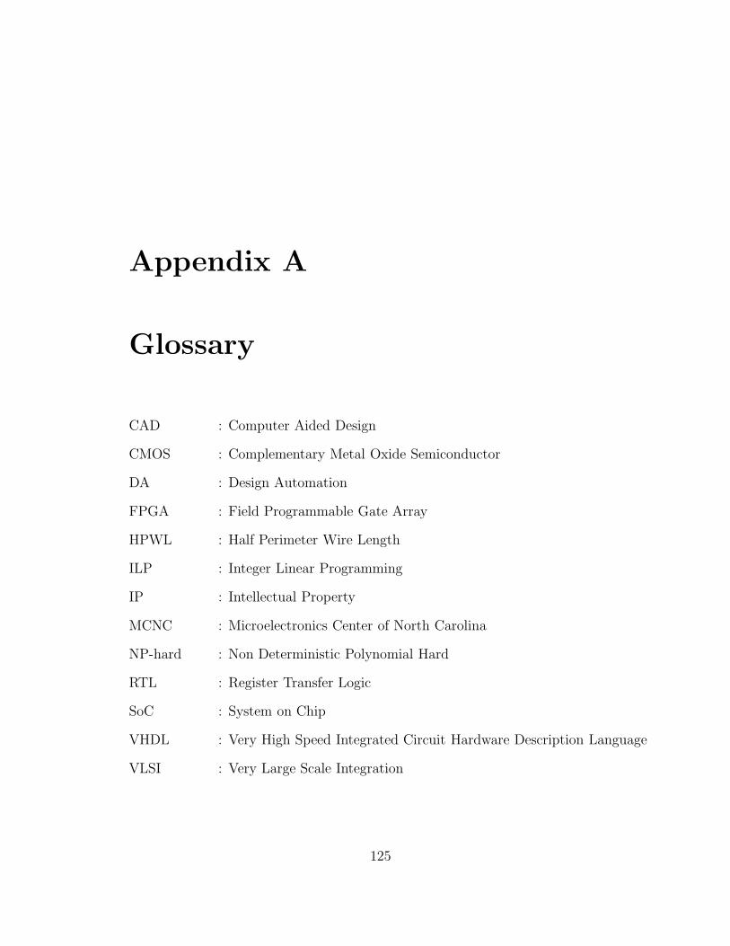
Appendix A
Glossary
CAD : Computer Aided Design
CMOS : Complementary Metal Oxide Semiconductor
DA : Design Automation
FPGA : Field Programmable Gate Array
HPWL : Half Perimeter Wire Length
ILP : Integer Linear Programming
IP : Intellectual Property
MCNC : Microelectronics Center of North Carolina
NP-hard : Non Deterministic Polynomial Hard
RTL : Register Transfer Logic
SoC : System on Chip
VHDL : Very High Speed Integrated Circuit Hardware Description Language
VLSI : Very Large Scale Integration
125

Appendix B
GA Parameter Tuning
Figure B.1 to Figure B.9 illustrate the relationships between the quality of the
placement solution (i.e. the total estimated wirelength) and different GA param-
eters on the flat level. Figure B.10 to Figure B.36 show the same relationships
between the quality of the placement solution and different GA parameters on the
clustering level-1, clustering level-2 and clustering level-3. All the results are ob-
tained by Pure Genetic Algorithm (i.e without using Local Search after GA) and
Pure Genetic Algorithm + Clustering Technique. Due to the large computation
time, we choose 30 as the largest population size and 100 as the largest genera-
tion size for all the testing circuits. The GA parameters include: population size,
generation size, mutation rate and crossover rate.
126

APPENDIX B. GA PARAMETER TUNING 127
B.1 Pure GA Results at Flat Level
60000
65000
70000
75000
80000
85000
90000
0 20 40 60 80 100
Wir
ele
ng
th
Generations
Fract pop:24 mu:1.2% cross:0.99
generations
60000
62000
64000
66000
68000
70000
72000
74000
10 15 20 25 30
Wir
ele
ng
th
Population
Fract gen:100 mu:1.2% cross:0.99
population
62000
64000
66000
68000
70000
72000
74000
0 0.5 1 1.5 2 2.5 3
Wir
ele
ng
th
Mutation Rate (%)
Fract gen:100 pop:24 cross:0.99
mutation rate
62000
64000
66000
68000
70000
72000
74000
76000
78000
80000
0.1 0.2 0.3 0.4 0.5 0.6 0.7 0.8 0.9 1
Wir
ele
ng
th
Crossover Rate
Fract gen:100 pop:24 mu:1.2%
crossover rate
Figure B.1: Parameters Tuning of Circuit Fract (at flat level)
For circuit Fract, as the generation size becomes large the quality of the placementsolution is improved. The larger population size produce better solution. 30 is thebest population size. The higher the crossover rate is, the better the quality of thesolution is. 0.99 is the best crossover rate. The mutation rate is varied irregularly.1.2% is the best mutation rate.

APPENDIX B. GA PARAMETER TUNING 128
2.2e+06
2.25e+06
2.3e+06
2.35e+06
2.4e+06
2.45e+06
2.5e+06
2.55e+06
2.6e+06
2.65e+06
0 20 40 60 80 100
Wir
ele
ng
th
Generations
Prim1 pop:24 mu:0.28% cross:0.99
generatons
2.2e+06
2.22e+06
2.24e+06
2.26e+06
2.28e+06
2.3e+06
2.32e+06
2.34e+06
2.36e+06
10 15 20 25 30W
ire
len
gth
Population
Prim1 gen:100 mu:0.28% cross:0.99
population
2.2e+06
2.25e+06
2.3e+06
2.35e+06
2.4e+06
2.45e+06
2.5e+06
0 0.1 0.2 0.3 0.4 0.5 0.6
Wir
ele
ng
th
Mutation Rate (%)
Prim1 gen:100 pop:24 cross:0.99
mutation rate
2.2e+06
2.25e+06
2.3e+06
2.35e+06
2.4e+06
2.45e+06
2.5e+06
0.1 0.2 0.3 0.4 0.5 0.6 0.7 0.8 0.9 1
Wir
ele
ng
th
Crossover Rate
Prim1 gen:100 pop:24 mu:0.28%
crossover rate
Figure B.2: Parameters Tuning of Circuit Prim1 (at flat level)
For circuit Prim1, as the generation size becomes large the quality of the placementsolution is improved. The larger population size produces better solution. 24 is thebest population size. The higher the crossover rate is, the better the quality ofthe solution is. 0.99 is the best crossover rate. The larger mutation rate producesbetter solution. 0.28% is the best mutation rate.

APPENDIX B. GA PARAMETER TUNING 129
2.2e+06
2.25e+06
2.3e+06
2.35e+06
2.4e+06
2.45e+06
2.5e+06
0 20 40 60 80 100
Wir
ele
ng
th
Generations
Struct pop:24 mu:0.36% cross:0.99
generatons
2.2e+06
2.22e+06
2.24e+06
2.26e+06
2.28e+06
2.3e+06
2.32e+06
2.34e+06
10 15 20 25 30W
ire
len
gth
Population
Struct gen:100 mu:0.36% cross:0.99
population
2.22e+06
2.24e+06
2.26e+06
2.28e+06
2.3e+06
2.32e+06
2.34e+06
2.36e+06
2.38e+06
2.4e+06
2.42e+06
0 0.05 0.1 0.15 0.2 0.25 0.3 0.35 0.4 0.45 0.5
Wir
ele
ng
th
Mutation Rate (%)
Struct gen:100 pop:24 cross:0.99
mutation rate
2.2e+06
2.25e+06
2.3e+06
2.35e+06
2.4e+06
2.45e+06
0.1 0.2 0.3 0.4 0.5 0.6 0.7 0.8 0.9 1
Wir
ele
ng
th
Crossover Rate
Struct gen:100 pop:24 mu:0.36%
crossover rate
Figure B.3: Parameters Tuning of Circuit Struct (at flat level)
For circuit Struct, as the generation size becomes large the quality of the placementsolution is improved. The larger population size produces better solution. 24 is thebest population size. The higher the crossover rate is, the better the quality ofthe solution is. 0.99 is the best crossover rate. The larger mutation rate producesbetter solution. 0.36% is the best mutation rate.

APPENDIX B. GA PARAMETER TUNING 130
5.4e+06
5.5e+06
5.6e+06
5.7e+06
5.8e+06
5.9e+06
6e+06
6.1e+06
0 20 40 60 80 100
Wir
ele
ng
th
Generations
Ind1 pop:24 mu:0.3 cross:0.9
generatons
5.3e+06
5.35e+06
5.4e+06
5.45e+06
5.5e+06
5.55e+06
5.6e+06
5.65e+06
10 15 20 25 30W
ire
len
gth
Population
Ind1 gen:100 mu:0.3 cross:0.9
population
5.4e+06
5.45e+06
5.5e+06
5.55e+06
5.6e+06
5.65e+06
5.7e+06
5.75e+06
5.8e+06
0 0.2 0.4 0.6 0.8 1 1.2 1.4 1.6 1.8
Wir
ele
ng
th
Mutation Rate (%)
Ind1 gen:100 pop:24 cross:0.99
mutation rate
5.4e+065.45e+065.5e+06
5.55e+065.6e+06
5.65e+065.7e+06
5.75e+065.8e+06
5.85e+065.9e+06
5.95e+06
0.1 0.2 0.3 0.4 0.5 0.6 0.7 0.8 0.9 1
Wir
ele
ng
th
Crossover Rate
Ind1 gen:100 pop:24 mu:0.3
crossover rate
Figure B.4: Parameters Tuning of Circuit Ind1 (at flat level)
For circuit Ind1, as the generation size becomes large the quality of the placementsolution is improved. The larger population size produces better solution. 30 isthe best population size. The higher the crossover rate is, the better the quality ofthe solution is. 0.99 is the best crossover rate. The larger mutation rate producesbetter solution. 0.3% is the best mutation rate.

APPENDIX B. GA PARAMETER TUNING 131
1.5e+07
1.52e+07
1.54e+07
1.56e+07
1.58e+07
1.6e+07
1.62e+07
1.64e+07
0 20 40 60 80 100
Wir
ele
ng
th
Generations
Prim2 pop:24 mu:0.5% cross:0.99
generatons
1.49e+07
1.5e+07
1.51e+07
1.52e+07
1.53e+07
1.54e+07
1.55e+07
10 15 20 25 30W
ire
len
gth
Population
Prim2 gen:100 mu:0.5% cross:0.99
population
1.5e+07
1.51e+07
1.52e+07
1.53e+07
1.54e+07
1.55e+07
1.56e+07
1.57e+07
1.58e+07
1.59e+07
1.6e+07
0 0.2 0.4 0.6 0.8 1 1.2 1.4 1.6 1.8
Wir
ele
ng
th
Mutation Rate (%)
Prim2 gen:100 pop:24 cross:0.99
mutation rate
1.5e+07
1.52e+07
1.54e+07
1.56e+07
1.58e+07
1.6e+07
1.62e+07
0.1 0.2 0.3 0.4 0.5 0.6 0.7 0.8 0.9 1
Wir
ele
ng
th
Crossover Rate
Prim2 gen:100 pop:24 mu:0.5%
crossover rate
Figure B.5: Parameters Tuning of Circuit Prim2 (at flat level)
For circuit Prim2, as the generation size becomes large the quality of the placementsolution is improved. The larger population size produces better solution. 30 is thebest population size. The higher the crossover rate is, the better the quality ofthe solution is. 0.99 is the best crossover rate. The larger mutation rate producesbetter solution. 0.5% is the best mutation rate.

APPENDIX B. GA PARAMETER TUNING 132
1.22e+07
1.23e+07
1.24e+07
1.25e+07
1.26e+07
1.27e+07
1.28e+07
1.29e+07
1.3e+07
1.31e+07
1.32e+07
0 20 40 60 80 100
Wir
ele
ng
th
Generations
Bio pop:24 mu:0.3 cross:0.9
generatons
1.22e+07
1.225e+07
1.23e+07
1.235e+07
1.24e+07
1.245e+07
1.25e+07
1.255e+07
10 15 20 25 30W
ire
len
gth
Population
Bio gen:100 mu:0.3 cross:0.9
population
1.22e+07
1.23e+07
1.24e+07
1.25e+07
1.26e+07
1.27e+07
1.28e+07
1.29e+07
0 0.2 0.4 0.6 0.8 1 1.2 1.4 1.6 1.8
Wir
ele
ng
th
Mutation Rate (%)
Bio gen:100 pop:24 cross:0.99
mutation rate
1.22e+07
1.23e+07
1.24e+07
1.25e+07
1.26e+07
1.27e+07
1.28e+07
1.29e+07
1.3e+07
0.1 0.2 0.3 0.4 0.5 0.6 0.7 0.8 0.9 1
Wir
ele
ng
th
Crossover Rate
Bio gen:100 pop:24 mu:0.3
crossover rate
Figure B.6: Parameters Tuning of Circuit Bio (at flat level)
For circuit Bio, as the generation size becomes large the quality of the placementsolution is improved. The larger population size produces better solution. 24 is thebest population size. The higher the crossover rate is, the better the quality of thesolution is. 0.99 is the best crossover rate. The mutation rate is varied irregularly.0.3% is the best mutation rate.

APPENDIX B. GA PARAMETER TUNING 133
8.85e+07
8.9e+07
8.95e+07
9e+07
9.05e+07
9.1e+07
9.15e+07
9.2e+07
9.25e+07
9.3e+07
0 20 40 60 80 100
Wir
ele
ng
th
Generations
Ind2 pop:24 mu:0.3 cross:0.9
generatons
8.86e+07
8.88e+07
8.9e+07
8.92e+07
8.94e+07
8.96e+07
8.98e+07
9e+07
9.02e+07
9.04e+07
9.06e+07
10 15 20 25 30W
ire
len
gth
Population
Ind2 gen:100 mu:0.3 cross:0.9
population
8.85e+07
8.9e+07
8.95e+07
9e+07
9.05e+07
9.1e+07
9.15e+07
9.2e+07
0 0.1 0.2 0.3 0.4 0.5 0.6 0.7 0.8 0.9 1
Wir
ele
ng
th
Mutation Rate (%)
Ind2 gen:100 pop:24 cross:0.99
mutation rate
8.85e+07
8.9e+07
8.95e+07
9e+07
9.05e+07
9.1e+07
9.15e+07
9.2e+07
0.1 0.2 0.3 0.4 0.5 0.6 0.7 0.8 0.9 1
Wir
ele
ng
th
Crossover Rate
Ind2 gen:100 pop:24 mu:0.3
crossover rate
Figure B.7: Parameters Tuning of Circuit Ind2 (at flat level)
For circuit Ind2, as the generation size becomes large the quality of the placementsolution is improved. The larger population size produces better solution. 24 isthe best population size. The higher the crossover rate is, the better the quality ofthe solution is. 0.99 is the best crossover rate. The larger mutation rate producesbetter solution. 0.2% is the best mutation rate.

APPENDIX B. GA PARAMETER TUNING 134
2.73e+08
2.74e+08
2.75e+08
2.76e+08
2.77e+08
2.78e+08
2.79e+08
2.8e+08
2.81e+08
2.82e+08
0 20 40 60 80 100
Wir
ele
ng
th
Generations
Ind3 pop:24 mu:0.1% cross:0.99
generatons
2.72e+08
2.73e+08
2.74e+08
2.75e+08
2.76e+08
2.77e+08
2.78e+08
10 15 20 25 30W
ire
len
gth
Population
Ind3 gen:100 mu:0.3 cross:0.9
population
2.73e+08
2.74e+08
2.75e+08
2.76e+08
2.77e+08
2.78e+08
2.79e+08
0 0.02 0.04 0.06 0.08 0.1 0.12 0.14 0.16 0.18 0.2
Wir
ele
ng
th
Mutation Rate (%)
Ind3 gen:100 pop:24 cross:0.99
mutation rate
2.73e+08
2.74e+08
2.75e+08
2.76e+08
2.77e+08
2.78e+08
2.79e+08
2.8e+08
2.81e+08
2.82e+08
0.1 0.2 0.3 0.4 0.5 0.6 0.7 0.8 0.9 1
Wir
ele
ng
th
Crossover Rate
Ind3 gen:100 pop:24 mu:0.3
crossover rate
Figure B.8: Parameters Tuning of Circuit Ind3 (at flat level)
For circuit Ind3, as the generation size becomes large the quality of the placementsolution is improved. The larger population size produces better solution. 20 isthe best population size. The higher the crossover rate is, the better the quality ofthe solution is. 0.99 is the best crossover rate. The larger mutation rate producesbetter solution. 0.1% is the best mutation rate.

APPENDIX B. GA PARAMETER TUNING 135
9.96e+07
9.98e+07
1e+08
1.002e+08
1.004e+08
1.006e+08
1.008e+08
1.01e+08
1.012e+08
1.014e+08
1.016e+08
0 20 40 60 80 100
Wir
ele
ng
th
Generations
avq_large pop:24 mu:0.02% cross:0.99
generatons
1.005e+08
1.006e+08
1.007e+08
1.008e+08
1.009e+08
1.01e+08
1.011e+08
1.012e+08
10 15 20 25 30W
ire
len
gth
Population
avq_large gen:100 mu:0.02% cross:0.99
population
9.97e+07
9.98e+07
9.99e+07
1e+08
1.001e+08
1.002e+08
1.003e+08
1.004e+08
1.005e+08
1.006e+08
1.007e+08
0 0.01 0.02 0.03 0.04 0.05 0.06 0.07 0.08 0.09 0.1
Wir
ele
ng
th
Mutation Rate (%)
avq_large gen:100 pop:24 cross:0.99
mutation rate
9.96e+079.98e+07
1e+081.002e+081.004e+081.006e+081.008e+08
1.01e+081.012e+081.014e+081.016e+081.018e+08
0.1 0.2 0.3 0.4 0.5 0.6 0.7 0.8 0.9 1
Wir
ele
ng
th
Crossover Rate
avq_large gen:100 pop:24 mu:0.02%
crossover rate
Figure B.9: Parameters Tuning of Circuit Avq.large (at flat level)
For circuit Avq.large, as the generation size becomes large the quality of the place-ment solution is improved. The larger population size produces better solution. 30is the best population size. The higher the crossover rate is, the better the qualityof the solution is. 0.99 is the best crossover rate. The larger mutation rate producesbetter solution. 0.02% is the best mutation rate.

APPENDIX B. GA PARAMETER TUNING 136
B.2 Pure GA Results at Clustering Level-1
58000
60000
62000
64000
66000
68000
70000
72000
74000
76000
78000
0 20 40 60 80 100
Wir
ele
ng
th
Generations
Fract (pop:24 mu:1.6% cross:0.99 clustering level-1)
generations
57000
58000
59000
60000
61000
62000
63000
64000
65000
10 15 20 25 30
Wir
ele
ng
th
Population
Fract (gen:100 mu:1.6% cross:0.99 clustering level-1)
population
58000
59000
60000
61000
62000
63000
64000
65000
66000
0 0.5 1 1.5 2 2.5 3
Wir
ele
ng
th
Mutation Rate (%)
Fract (gen:100 pop:24 cross:0.99 clusternig level-1)
mutation rate
58000
60000
62000
64000
66000
68000
70000
72000
74000
0.1 0.2 0.3 0.4 0.5 0.6 0.7 0.8 0.9 1
Wir
ele
ng
th
Crossover Rate
Fract (gen:100 pop:24 mu:1.6% clustering level-1)
crossover rate
Figure B.10: Parameters Tuning of Circuit Fract (at clustering level-1)
For circuit Fract, as the generation size becomes large the quality of the placementsolution is improved. The larger population size produce better solution. 20 is thebest population size. The higher the crossover rate is, the better the quality of thesolution is. 0.99 is the best crossover rate. The mutation rate is varied irregularly.1.6% is the best mutation rate.

APPENDIX B. GA PARAMETER TUNING 137
2.7e+06
2.75e+06
2.8e+06
2.85e+06
2.9e+06
2.95e+06
3e+06
3.05e+06
3.1e+06
3.15e+06
0 20 40 60 80 100
Wir
ele
ng
th
Generations
Prim1 (pop:24 mu:0.36% cross:0.99 clustering level-1)
generatons
2.7e+06
2.72e+06
2.74e+06
2.76e+06
2.78e+06
2.8e+06
2.82e+06
2.84e+06
2.86e+06
2.88e+06
10 15 20 25 30W
ire
len
gth
Population
Prim1 (gen:100 mu:0.36% cross:0.99 clustering level-1)
population
2.7e+06
2.75e+06
2.8e+06
2.85e+06
2.9e+06
2.95e+06
3e+06
0 0.05 0.1 0.15 0.2 0.25 0.3 0.35 0.4
Wir
ele
ng
th
Mutation Rate (%)
Prim1 (gen:100 pop:24 cross:0.99 clustering level-1)
mutation rate
2.7e+06
2.75e+06
2.8e+06
2.85e+06
2.9e+06
2.95e+06
3e+06
3.05e+06
0.1 0.2 0.3 0.4 0.5 0.6 0.7 0.8 0.9 1
Wir
ele
ng
th
Crossover Rate
Prim1 (gen:100 pop:24 mu:0.36% clustering level-1)
crossover rate
Figure B.11: Parameters Tuning of Circuit Prim1 (at clustering level-1)
For circuit Prim1, as the generation size becomes large the quality of the placementsolution is improved. The larger population size produce better solution. 24 is thebest population size. The higher the crossover rate is, the better the quality ofthe solution is. 0.99 is the best crossover rate. The larger mutation rate producesbetter solution. 0.36% is the best mutation rate.

APPENDIX B. GA PARAMETER TUNING 138
2.7e+06
2.75e+06
2.8e+06
2.85e+06
2.9e+06
2.95e+06
3e+06
0 20 40 60 80 100
Wir
ele
ng
th
Generations
Struct (pop:24 mu:0.24% cross:0.99 clustering level-1)
generatons
2.64e+06
2.66e+06
2.68e+06
2.7e+06
2.72e+06
2.74e+06
2.76e+06
2.78e+06
2.8e+06
2.82e+06
10 15 20 25 30W
ire
len
gth
Population
Struct (gen:100 mu:0.24% cross:0.99 clustering level-1)
population
2.7e+06
2.75e+06
2.8e+06
2.85e+06
2.9e+06
2.95e+06
0 0.05 0.1 0.15 0.2 0.25 0.3 0.35 0.4 0.45 0.5
Wir
ele
ng
th
Mutation Rate (%)
Struct (gen:100 pop:24 cross:0.99 clustering level-1)
mutation rate
2.7e+06
2.75e+06
2.8e+06
2.85e+06
2.9e+06
2.95e+06
0.1 0.2 0.3 0.4 0.5 0.6 0.7 0.8 0.9 1
Wir
ele
ng
th
Crossover Rate
Struct (gen:100 pop:24 mu:0.24% clustering level-1)
crossover rate
Figure B.12: Parameters Tuning of Circuit Struct (at clustering level-1)
For circuit Struct, as the generation size becomes large the quality of the placementsolution is improved. The larger population size produce better solution. 30 is thebest population size. The higher the crossover rate is, the better the quality ofthe solution is. 0.99 is the best crossover rate. The larger mutation rate producesbetter solution. 0.24% is the best mutation rate.

APPENDIX B. GA PARAMETER TUNING 139
5.5e+06
5.6e+06
5.7e+06
5.8e+06
5.9e+06
6e+06
6.1e+06
6.2e+06
6.3e+06
0 20 40 60 80 100
Wir
ele
ng
th
Generations
Ind1 ( pop:24 mu:0.5% cross:0.99 clustering level-1)
generatons
5.54e+06
5.56e+06
5.58e+06
5.6e+06
5.62e+06
5.64e+06
5.66e+06
5.68e+06
5.7e+06
5.72e+06
10 15 20 25 30W
ire
len
gth
Population
Ind1 ( gen:100 mu:0.5 cross:0.99 clustering level-1)
population
5.5e+06
5.6e+06
5.7e+06
5.8e+06
5.9e+06
6e+06
6.1e+06
0 0.2 0.4 0.6 0.8 1 1.2 1.4 1.6 1.8
Wir
ele
ng
th
Mutation Rate (%)
Ind1 (gen:100 pop:24 cross:0.99 clustering level-1)
mutation rate
5.5e+06
5.6e+06
5.7e+06
5.8e+06
5.9e+06
6e+06
6.1e+06
0.1 0.2 0.3 0.4 0.5 0.6 0.7 0.8 0.9 1
Wir
ele
ng
th
Crossover Rate
Ind1 (gen:100 pop:24 mu:0.5% clustering level-1)
crossover rate
Figure B.13: Parameters Tuning of Circuit Ind1 (at clustering level-1)
For circuit Ind1, as the generation size becomes large the quality of the placementsolution is improved. The larger population size produce better solution. 30 is thebest population size. The higher the crossover rate is, the better the quality of thesolution is. 0.9 is the best crossover rate. The larger mutation rate produces bettersolution. 0.5% is the best mutation rate.

APPENDIX B. GA PARAMETER TUNING 140
1.78e+07
1.8e+07
1.82e+07
1.84e+07
1.86e+07
1.88e+07
1.9e+07
1.92e+07
1.94e+07
0 20 40 60 80 100
Wir
ele
ng
th
Generations
Prim2 ( pop:24 mu:0.5% cross:0.99 clustering level-1)
generatons
1.79e+07
1.795e+07
1.8e+07
1.805e+07
1.81e+07
1.815e+07
1.82e+07
1.825e+07
1.83e+07
10 15 20 25 30W
ire
len
gth
Population
Prim2 ( gen:100 mu:0.5% cross:0.99 clustering level-1)
population
1.79e+07
1.8e+07
1.81e+07
1.82e+07
1.83e+07
1.84e+07
1.85e+07
1.86e+07
1.87e+07
1.88e+07
1.89e+07
0 0.2 0.4 0.6 0.8 1 1.2 1.4 1.6 1.8
Wir
ele
ng
th
Mutation Rate (%)
Prim2 ( gen:100 pop:24 cross:0.99 clustering level-1)
mutation rate
1.78e+07
1.8e+07
1.82e+07
1.84e+07
1.86e+07
1.88e+07
1.9e+07
1.92e+07
0.1 0.2 0.3 0.4 0.5 0.6 0.7 0.8 0.9 1
Wir
ele
ng
th
Crossover Rate
Prim2 ( gen:100 pop:24 mu:0.5% clustering level-1)
crossover rate
Figure B.14: Parameters Tuning of Circuit Prim2 (at clustering level-1)
For circuit Prim2, as the generation size becomes large the quality of the placementsolution is improved. The larger population size produce better solution. 24 is thebest population size. The higher the crossover rate is, the better the quality ofthe solution is. 0.99 is the best crossover rate. The larger mutation rate producesbetter solution. 0.5% is the best mutation rate.

APPENDIX B. GA PARAMETER TUNING 141
1.54e+071.55e+071.56e+071.57e+071.58e+071.59e+071.6e+07
1.61e+071.62e+071.63e+071.64e+071.65e+07
0 20 40 60 80 100
Wir
ele
ng
th
Generations
Bio ( pop:24 mu:0.5% cross:0.99 clustering level-1)
generatons
1.54e+07
1.545e+07
1.55e+07
1.555e+07
1.56e+07
1.565e+07
1.57e+07
1.575e+07
10 15 20 25 30W
ire
len
gth
Population
Bio ( gen:100 mu:0.5% cross:0.99 clustering level-1)
population
1.54e+07
1.55e+07
1.56e+07
1.57e+07
1.58e+07
1.59e+07
1.6e+07
1.61e+07
1.62e+07
0 0.2 0.4 0.6 0.8 1 1.2 1.4 1.6 1.8
Wir
ele
ng
th
Mutation Rate (%)
Bio ( gen:100 pop:24 cross:0.99 clustering level-1)
mutation rate
1.54e+07
1.55e+07
1.56e+07
1.57e+07
1.58e+07
1.59e+07
1.6e+07
1.61e+07
1.62e+07
1.63e+07
1.64e+07
0.1 0.2 0.3 0.4 0.5 0.6 0.7 0.8 0.9 1
Wir
ele
ng
th
Crossover Rate
Bio ( gen:100 pop:24 mu:0.5% clustering level-1)
crossover rate
Figure B.15: Parameters Tuning of Circuit Bio (at clustering level-1)
For circuit Bio, as the generation size becomes large the quality of the placementsolution is improved. 30 is the best population size. 0.99 is the best crossover rate.The mutation rate is varied irregularly. 0.5% is the best mutation rate.

APPENDIX B. GA PARAMETER TUNING 142
1.2e+08
1.21e+08
1.22e+08
1.23e+08
1.24e+08
1.25e+08
1.26e+08
0 20 40 60 80 100
Wir
ele
ng
th
Generations
Ind2 ( pop:24 mu:0.5% cross:0.99 clustering level-1)
generatons
1.202e+08
1.204e+08
1.206e+08
1.208e+08
1.21e+08
1.212e+08
1.214e+08
1.216e+08
1.218e+08
1.22e+08
10 15 20 25 30W
ire
len
gth
Population
Ind2 ( gen:100 mu:0.5% cross:0.99 clustering level-1)
population
1.2e+08
1.205e+08
1.21e+08
1.215e+08
1.22e+08
1.225e+08
1.23e+08
1.235e+08
1.24e+08
1.245e+08
1.25e+08
0 0.2 0.4 0.6 0.8 1 1.2 1.4 1.6 1.8
Wir
ele
ng
th
Mutation Rate (%)
Ind2 ( gen:100 pop:24 cross:0.99 clustering level-1)
mutation rate
1.2e+08
1.205e+08
1.21e+08
1.215e+08
1.22e+08
1.225e+08
1.23e+08
1.235e+08
1.24e+08
1.245e+08
0.1 0.2 0.3 0.4 0.5 0.6 0.7 0.8 0.9 1
Wir
ele
ng
th
Crossover Rate
Ind2 ( gen:100 pop:24 mu:0.5% clustering level-1)
crossover rate
Figure B.16: Parameters Tuning of Circuit Ind2 (at clustring level-1)
For circuit Ind2, as the generation size becomes large the quality of the placementsolution is improved. The larger population size produce better solution. 30 is thebest population size. The higher the crossover rate is, the better the quality of thesolution is. 0.99 is the best crossover rate. The mutation rate is varied irregularly.0.5% is the best mutation rate.

APPENDIX B. GA PARAMETER TUNING 143
4.16e+08
4.18e+08
4.2e+08
4.22e+08
4.24e+08
4.26e+08
4.28e+08
4.3e+08
4.32e+08
0 20 40 60 80 100
Wir
ele
ng
th
Generations
Ind3 ( pop:24 mu:0.5% cross:0.99 clustering level-1)
generatons
4.16e+08
4.17e+08
4.18e+08
4.19e+08
4.2e+08
4.21e+08
4.22e+08
4.23e+08
10 15 20 25 30W
ire
len
gth
Population
Ind3 ( gen:100 mu:0.5% cross:0.99 clustering level-1)
population
4.17e+08
4.18e+08
4.19e+08
4.2e+08
4.21e+08
4.22e+08
4.23e+08
4.24e+08
4.25e+08
4.26e+08
4.27e+08
0 0.2 0.4 0.6 0.8 1 1.2 1.4 1.6 1.8
Wir
ele
ng
th
Mutation Rate (%)
Ind3 ( gen:100 pop:24 cross:0.99 clustering level-1)
mutation rate
4.17e+08
4.18e+08
4.19e+08
4.2e+08
4.21e+08
4.22e+08
4.23e+08
4.24e+08
4.25e+08
4.26e+08
4.27e+08
0.1 0.2 0.3 0.4 0.5 0.6 0.7 0.8 0.9 1
Wir
ele
ng
th
Crossover Rate
Ind3 ( gen:100 pop:24 mu:0.5% clustering level-1)
crossover rate
Figure B.17: Parameters Tuning of Circuit Ind3 (at clustering level-1)
For circuit Ind3, as the generation size becomes large the quality of the placementsolution is improved. The larger population size produce better solution. 30 is thebest population size. The higher the crossover rate is, the better the quality of thesolution is. 0.99 is the best crossover rate. The mutation rate is varied irregularly.0.5% is the best mutation rate.

APPENDIX B. GA PARAMETER TUNING 144
1.29e+08
1.295e+08
1.3e+08
1.305e+08
1.31e+08
1.315e+08
1.32e+08
1.325e+08
1.33e+08
1.335e+08
0 20 40 60 80 100
Wir
ele
ng
th
Generations
avq_large ( pop:24 mu:0.5% cross:0.99 clustering level-1)
generatons
1.285e+08
1.29e+08
1.295e+08
1.3e+08
1.305e+08
1.31e+08
1.315e+08
1.32e+08
1.325e+08
10 15 20 25 30W
ire
len
gth
Population
avq_large ( gen:100 mu:0.5% cross:0.99 clustering level-1)
population
1.29e+08
1.295e+08
1.3e+08
1.305e+08
1.31e+08
1.315e+08
1.32e+08
1.325e+08
0 0.05 0.1 0.15 0.2 0.25 0.3 0.35 0.4 0.45 0.5
Wir
ele
ng
th
Mutation Rate (%)
avq_large ( gen:100 pop:24 cross:0.99 clustering level-1)
mutation rate
1.29e+08
1.295e+08
1.3e+08
1.305e+08
1.31e+08
1.315e+08
1.32e+08
1.325e+08
1.33e+08
1.335e+08
1.34e+08
0.1 0.2 0.3 0.4 0.5 0.6 0.7 0.8 0.9 1
Wir
ele
ng
th
Crossover Rate
avq_large ( gen:100 pop:24 mu:0.5% clustering level-1)
crossover rate
Figure B.18: Parameters Tuning of Circuit Avq.large (at clustering level-1)
For circuit Avq.large, as the generation size becomes large the quality of the place-ment solution is improved. The larger population size produce better solution. 30is the best population size. The higher the crossover rate is, the better the qualityof the solution is. 0.99 is the best crossover rate. The larger mutation rate producesbetter solution. 0.5% is the best mutation rate.

APPENDIX B. GA PARAMETER TUNING 145
B.3 Pure GA Results at Clustering Level-2
50000
55000
60000
65000
70000
75000
80000
0 20 40 60 80 100
Wir
ele
ng
th
Generations
Fract (pop:24 mu:3% cross:0.99 clustering level-2)
generations
53000
54000
55000
56000
57000
58000
59000
60000
61000
62000
10 15 20 25 30
Wir
ele
ng
th
Population
Fract (gen:100 mu:3% cross:0.99 clustering level-2)
population
52000
54000
56000
58000
60000
62000
64000
66000
0 0.5 1 1.5 2 2.5 3
Wir
ele
ng
th
Mutation Rate (%)
Fract (gen:100 pop:24 cross:0.99 clustering-2)
mutation rate
52000
54000
56000
58000
60000
62000
64000
66000
68000
70000
0.1 0.2 0.3 0.4 0.5 0.6 0.7 0.8 0.9 1
Wir
ele
ng
th
Crossover Rate
Fract (gen:100 pop:24 mu:3% clustering level-2)
crossover rate
Figure B.19: Parameters Tuning of Circuit Fract (at clustering level-2)
For circuit Fract, as the generation size becomes large the quality of the placementsolution is improved. The larger population size produce better solution. 24 is thebest population size. The higher the crossover rate is, the better the quality of thesolution is. 0.99 is the best crossover rate. The mutation rate is varied irregularly.3% is the best mutation rate.

APPENDIX B. GA PARAMETER TUNING 146
2.35e+06
2.4e+06
2.45e+06
2.5e+06
2.55e+06
2.6e+06
2.65e+06
2.7e+06
2.75e+06
0 20 40 60 80 100
Wir
ele
ng
th
Generations
Prim1 (pop:24 mu:0.4% cross:0.99 clustering level-2)
generatons
2.3e+06
2.35e+06
2.4e+06
2.45e+06
2.5e+06
2.55e+06
2.6e+06
10 15 20 25 30W
ire
len
gth
Population
Prim1 (gen:100 mu:0.4% cross:0.99 clustering level-2)
population
2.35e+06
2.4e+06
2.45e+06
2.5e+06
2.55e+06
2.6e+06
2.65e+06
0 0.05 0.1 0.15 0.2 0.25 0.3 0.35 0.4
Wir
ele
ng
th
Mutation Rate (%)
Prim1 (gen:100 pop:24 cross:0.99 clustering level-2)
mutation rate
2.35e+06
2.4e+06
2.45e+06
2.5e+06
2.55e+06
2.6e+06
2.65e+06
2.7e+06
0.1 0.2 0.3 0.4 0.5 0.6 0.7 0.8 0.9 1
Wir
ele
ng
th
Crossover Rate
Prim1 (gen:100 pop:24 mu:0.4% clustering level-2)
crossover rate
Figure B.20: Parameters Tuning of Circuit Prim1 (at clustering level-2)
For circuit Prim1, as the generation size becomes large the quality of the placementsolution is improved. The larger population size produce better solution. 30 is thebest population size. The higher the crossover rate is, the better the quality of thesolution is. 0.99 is the best crossover rate. The mutation rate is varied irregularly.0.4% is the best mutation rate.

APPENDIX B. GA PARAMETER TUNING 147
2.1e+06
2.15e+06
2.2e+06
2.25e+06
2.3e+06
2.35e+06
2.4e+06
0 20 40 60 80 100
Wir
ele
ng
th
Generations
Struct (pop:24 mu:0.4% cross:0.99 clustering level-2)
generatons
2.09e+06
2.1e+06
2.11e+06
2.12e+06
2.13e+06
2.14e+06
2.15e+06
2.16e+06
2.17e+06
2.18e+06
2.19e+06
10 15 20 25 30W
ire
len
gth
Population
Struct (gen:100 mu:0.4% cross:0.99 clustering level-2)
population
2.1e+06
2.15e+06
2.2e+06
2.25e+06
2.3e+06
2.35e+06
0 0.05 0.1 0.15 0.2 0.25 0.3 0.35 0.4
Wir
ele
ng
th
Mutation Rate (%)
Struct (gen:100 pop:24 cross:0.99 clustering level-2)
mutation rate
2.1e+06
2.15e+06
2.2e+06
2.25e+06
2.3e+06
2.35e+06
2.4e+06
0.1 0.2 0.3 0.4 0.5 0.6 0.7 0.8 0.9 1
Wir
ele
ng
th
Crossover Rate
Struct (gen:100 pop:24 mu:0.4% clustering level-2
crossover rate
Figure B.21: Parameters Tuning of Circuit Struct (at clustering level-2)
For circuit Struct, as the generation size becomes large the quality of the placementsolution is improved. The larger population size produce better solution. 30 is thebest population size. The higher the crossover rate is, the better the quality ofthe solution is. 0.99 is the best crossover rate. The larger mutation rate producesbetter solution. 0.4% is the best mutation rate.

APPENDIX B. GA PARAMETER TUNING 148
4.8e+06
4.9e+06
5e+06
5.1e+06
5.2e+06
5.3e+06
5.4e+06
5.5e+06
0 20 40 60 80 100
Wir
ele
ng
th
Generations
Ind1 (pop:24 mu:0.3 cross:0.9 clustering level-2)
generatons
5.08e+06
5.1e+06
5.12e+06
5.14e+06
5.16e+06
5.18e+06
5.2e+06
5.22e+06
5.24e+06
5.26e+06
10 15 20 25 30W
ire
len
gth
Population
Ind1 (gen:100 mu:0.3 cross:0.9 clustering level-2)
population
4.8e+06
4.85e+06
4.9e+06
4.95e+06
5e+06
5.05e+06
5.1e+06
5.15e+06
5.2e+06
5.25e+06
5.3e+06
0 0.2 0.4 0.6 0.8 1 1.2 1.4 1.6 1.8
Wir
ele
ng
th
Mutation Rate (%)
Ind1 (gen:100 pop:24 cross:0.99 clustering level-2)
mutation rate
4.8e+06
4.85e+06
4.9e+06
4.95e+06
5e+06
5.05e+06
5.1e+06
5.15e+06
5.2e+06
5.25e+06
5.3e+06
0.1 0.2 0.3 0.4 0.5 0.6 0.7 0.8 0.9 1
Wir
ele
ng
th
Crossover Rate
Ind1 (gen:100 pop:24 mu:0.5% clusterign level-2)
crossover rate
Figure B.22: Parameters Tuning of Circuit Ind1 (at clustering level-2)
For circuit Ind1, as the generation size becomes large the quality of the placementsolution is improved. The larger population size produce better solution. 30 is thebest population size. The higher the crossover rate is, the better the quality of thesolution is. 0.99 is the best crossover rate. The mutation rate is varied irregularly.0.5% is the best mutation rate.

APPENDIX B. GA PARAMETER TUNING 149
1.5e+07
1.52e+07
1.54e+07
1.56e+07
1.58e+07
1.6e+07
1.62e+07
1.64e+07
0 20 40 60 80 100
Wir
ele
ng
th
Generations
Prim2 (pop:24 mu:0.5% cross:0.99 clustering level-2)
generatons
1.49e+071.495e+07
1.5e+071.505e+07
1.51e+071.515e+07
1.52e+071.525e+07
1.53e+071.535e+07
1.54e+071.545e+07
10 15 20 25 30W
ire
len
gth
Population
Prim2 (gen:100 mu:0.5% cross:0.9 clustering level-2)
population
1.51e+07
1.52e+07
1.53e+07
1.54e+07
1.55e+07
1.56e+07
1.57e+07
1.58e+07
1.59e+07
1.6e+07
0 0.2 0.4 0.6 0.8 1 1.2 1.4 1.6 1.8
Wir
ele
ng
th
Mutation Rate (%)
Prim2 (gen:100 pop:24 cross:0.99 clustering level-2)
mutation rate
1.51e+07
1.52e+07
1.53e+07
1.54e+07
1.55e+07
1.56e+07
1.57e+07
1.58e+07
1.59e+07
1.6e+07
1.61e+07
0.1 0.2 0.3 0.4 0.5 0.6 0.7 0.8 0.9 1
Wir
ele
ng
th
Crossover Rate
Prim2 (gen:100 pop:24 mu:0.5% clustering level-2)
crossover rate
Figure B.23: Parameters Tuning of Circuit Prim2 (at clustering level-2)
For circuit Prim2, as the generation size becomes large the quality of the placementsolution is improved. The larger population size produce better solution. 30 is thebest population size. The higher the crossover rate is, the better the quality ofthe solution is. 0.99 is the best crossover rate. The larger mutation rate producesbetter solution. 0.5% is the best mutation rate.

APPENDIX B. GA PARAMETER TUNING 150
1.16e+07
1.17e+07
1.18e+07
1.19e+07
1.2e+07
1.21e+07
1.22e+07
1.23e+07
1.24e+07
1.25e+07
0 20 40 60 80 100
Wir
ele
ng
th
Generations
Bio (pop:24 mu:1.0% cross:0.99 clustering level-2)
generatons
1.15e+07
1.155e+07
1.16e+07
1.165e+07
1.17e+07
1.175e+07
1.18e+07
10 15 20 25 30W
ire
len
gth
Population
Bio (gen:100 mu:1.0% cross:0.99 clustering level-2)
population
1.16e+07
1.17e+07
1.18e+07
1.19e+07
1.2e+07
1.21e+07
1.22e+07
0 0.2 0.4 0.6 0.8 1 1.2 1.4 1.6 1.8
Wir
ele
ng
th
Mutation Rate (%)
Bio (gen:100 pop:24 cross:0.99 clustering level-2)
mutation rate
1.16e+07
1.17e+07
1.18e+07
1.19e+07
1.2e+07
1.21e+07
1.22e+07
1.23e+07
0.1 0.2 0.3 0.4 0.5 0.6 0.7 0.8 0.9 1
Wir
ele
ng
th
Crossover Rate
Bio (gen:100 pop:24 mu:1.0% clustering level-2)
crossover rate
Figure B.24: Parameters Tuning of Circuit Bio (at clustering level-2)
For circuit Bio, as the generation size becomes large the quality of the placementsolution is improved. The larger population size produce better solution. 30 is thebest population size. The higher the crossover rate is, the better the quality of thesolution is. 0.99 is the best crossover rate. The mutation rate is varied irregularly.1% is the best mutation rate.
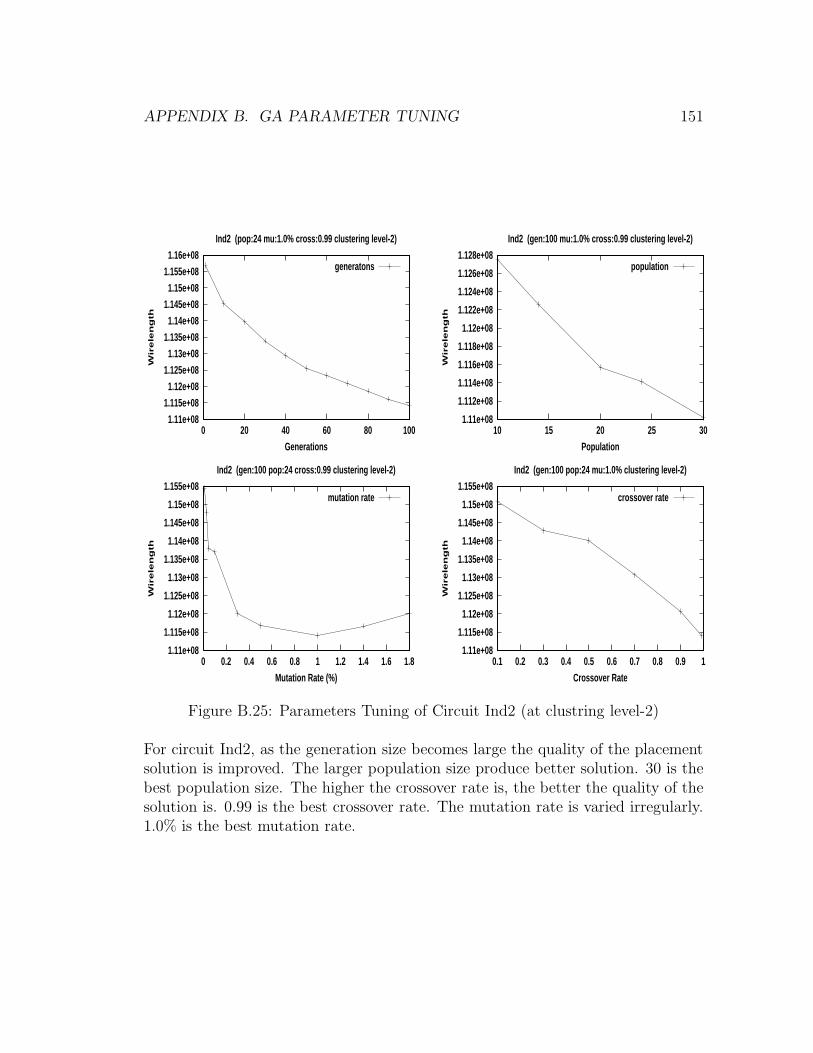
APPENDIX B. GA PARAMETER TUNING 151
1.11e+08
1.115e+08
1.12e+08
1.125e+08
1.13e+08
1.135e+08
1.14e+08
1.145e+08
1.15e+08
1.155e+08
1.16e+08
0 20 40 60 80 100
Wir
ele
ng
th
Generations
Ind2 (pop:24 mu:1.0% cross:0.99 clustering level-2)
generatons
1.11e+08
1.112e+08
1.114e+08
1.116e+08
1.118e+08
1.12e+08
1.122e+08
1.124e+08
1.126e+08
1.128e+08
10 15 20 25 30W
ire
len
gth
Population
Ind2 (gen:100 mu:1.0% cross:0.99 clustering level-2)
population
1.11e+08
1.115e+08
1.12e+08
1.125e+08
1.13e+08
1.135e+08
1.14e+08
1.145e+08
1.15e+08
1.155e+08
0 0.2 0.4 0.6 0.8 1 1.2 1.4 1.6 1.8
Wir
ele
ng
th
Mutation Rate (%)
Ind2 (gen:100 pop:24 cross:0.99 clustering level-2)
mutation rate
1.11e+08
1.115e+08
1.12e+08
1.125e+08
1.13e+08
1.135e+08
1.14e+08
1.145e+08
1.15e+08
1.155e+08
0.1 0.2 0.3 0.4 0.5 0.6 0.7 0.8 0.9 1
Wir
ele
ng
th
Crossover Rate
Ind2 (gen:100 pop:24 mu:1.0% clustering level-2)
crossover rate
Figure B.25: Parameters Tuning of Circuit Ind2 (at clustring level-2)
For circuit Ind2, as the generation size becomes large the quality of the placementsolution is improved. The larger population size produce better solution. 30 is thebest population size. The higher the crossover rate is, the better the quality of thesolution is. 0.99 is the best crossover rate. The mutation rate is varied irregularly.1.0% is the best mutation rate.

APPENDIX B. GA PARAMETER TUNING 152
3.7e+08
3.72e+08
3.74e+08
3.76e+08
3.78e+08
3.8e+08
3.82e+08
3.84e+08
3.86e+08
0 20 40 60 80 100
Wir
ele
ng
th
Generations
Ind3 (pop:24 mu:0.5% cross:0.99 clustering level-2)
generatons
3.7e+08
3.72e+08
3.74e+08
3.76e+08
3.78e+08
3.8e+08
3.82e+08
3.84e+08
10 15 20 25 30W
ire
len
gth
Population
Ind3 (gen:100 mu:0.5% cross:0.99 clustering level-2)
population
3.7e+08
3.72e+08
3.74e+08
3.76e+08
3.78e+08
3.8e+08
3.82e+08
3.84e+08
0 0.2 0.4 0.6 0.8 1 1.2 1.4 1.6 1.8
Wir
ele
ng
th
Mutation Rate (%)
Ind3 (gen:100 pop:24 cross:0.99 clustering level-2)
mutation rate
3.7e+08
3.72e+08
3.74e+08
3.76e+08
3.78e+08
3.8e+08
3.82e+08
0.1 0.2 0.3 0.4 0.5 0.6 0.7 0.8 0.9 1
Wir
ele
ng
th
Crossover Rate
Ind3 (gen:100 pop:24 mu:0.5% clustering level-2)
crossover rate
Figure B.26: Parameters Tuning of Circuit Ind3 (at clustering level-2)
For circuit Ind3, as the generation size becomes large the quality of the placementsolution is improved. The larger population size produce better solution. 30 is thebest population size. The higher the crossover rate is, the better the quality of thesolution is. 0.9 is the best crossover rate. The mutation rate is varied irregularly.0.5% is the best mutation rate.

APPENDIX B. GA PARAMETER TUNING 153
1.135e+08
1.14e+08
1.145e+08
1.15e+08
1.155e+08
1.16e+08
1.165e+08
1.17e+08
1.175e+08
0 20 40 60 80 100
Wir
ele
ng
th
Generations
avq_large (pop:24 mu:1.0% cross:0.99 clustering level-2)
generatons
1.125e+08
1.13e+08
1.135e+08
1.14e+08
1.145e+08
1.15e+08
1.155e+08
1.16e+08
1.165e+08
1.17e+08
1.175e+08
10 15 20 25 30W
ire
len
gth
Population
avq_large (gen:100 mu:1.0% cross:0.99 clustering level-2)
population
1.135e+08
1.14e+08
1.145e+08
1.15e+08
1.155e+08
1.16e+08
1.165e+08
1.17e+08
0 0.2 0.4 0.6 0.8 1 1.2 1.4 1.6 1.8
Wir
ele
ng
th
Mutation Rate (%)
avq_large (gen:100 pop:24 cross:0.99 clustering level-2)
mutation rate
1.13e+08
1.14e+08
1.15e+08
1.16e+08
1.17e+08
1.18e+08
1.19e+08
1.2e+08
0.1 0.2 0.3 0.4 0.5 0.6 0.7 0.8 0.9 1
Wir
ele
ng
th
Crossover Rate
avq_large (gen:100 pop:24 mu:1.0% clustering level-2)
crossover rate
Figure B.27: Parameters Tuning of Circuit Avq.large (at clustering level-2)
For circuit Avq.large, as the generation size becomes large the quality of the place-ment solution is improved. The larger population size produce better solution. 30is the best population size. The higher the crossover rate is, the better the qual-ity of the solution is. 0.9 is the best crossover rate. The mutation rate is variedirregularly. 1.0% is the best mutation rate.

APPENDIX B. GA PARAMETER TUNING 154
B.4 Pure GA Results at Clustering Level-3
460004800050000520005400056000580006000062000640006600068000
0 20 40 60 80 100
Wir
ele
ng
th
Generations
Fract (pop:24 mu:3% cross:0.99 clustering level-3)
generations
47000
48000
49000
50000
51000
52000
53000
54000
10 15 20 25 30
Wir
ele
ng
th
Population
Fract (gen:100 mu:1% cross:0.99 clustering level-3)
population
46000
48000
50000
52000
54000
56000
58000
60000
0 0.5 1 1.5 2 2.5 3
Wir
ele
ng
th
Mutation Rate (%)
Fract (gen:100 pop:24 cross:0.99 clustering level-3)
mutation rate
46000
48000
50000
52000
54000
56000
58000
60000
62000
0.1 0.2 0.3 0.4 0.5 0.6 0.7 0.8 0.9 1
Wir
ele
ng
th
Crossover Rate
Fract (gen:100 pop:24 mu:1% clustering level-3)
crossover rate
Figure B.28: Parameters Tuning of Circuit Fract (at clustering level-3)
For circuit Fract, as the generation size becomes large the quality of the placementsolution is improved. The larger population size produce better solution. 24 is thebest population size. The higher the crossover rate is, the better the quality of thesolution is. 0.9 is the best crossover rate. The larger mutation rate produces bettersolution. 1% is the best mutation rate.

APPENDIX B. GA PARAMETER TUNING 155
2.1e+06
2.15e+06
2.2e+06
2.25e+06
2.3e+06
2.35e+06
2.4e+06
2.45e+06
2.5e+06
2.55e+06
0 20 40 60 80 100
Wir
ele
ng
th
Generations
Prim1 (pop:24 mu:0.4% cross:0.99 clustering level-3)
generatons
2.2e+06
2.22e+06
2.24e+06
2.26e+06
2.28e+06
2.3e+06
2.32e+06
2.34e+06
2.36e+06
10 15 20 25 30W
ire
len
gth
Population
Prim1 (gen:100 mu:0.4% cross:0.99 clustering level-3)
population
2.1e+06
2.15e+06
2.2e+06
2.25e+06
2.3e+06
2.35e+06
2.4e+06
0 0.05 0.1 0.15 0.2 0.25 0.3 0.35 0.4
Wir
ele
ng
th
Mutation Rate (%)
Prim1 (gen:100 pop:24 cross:0.99 clustering level-3)
mutation rate
2.15e+06
2.2e+06
2.25e+06
2.3e+06
2.35e+06
2.4e+06
2.45e+06
0.1 0.2 0.3 0.4 0.5 0.6 0.7 0.8 0.9 1
Wir
ele
ng
th
Crossover Rate
Prim1 (gen:100 pop:24 mu:0.4% clustering level-3)
crossover rate
Figure B.29: Parameters Tuning of Circuit Prim1 (at clustering level-3)
For circuit Prim1, as the generation size becomes large the quality of the placementsolution is improved. The larger population size produce better solution. 30 is thebest population size. The higher the crossover rate is, the better the quality of thesolution is. 0.99 is the best crossover rate. The mutation rate is varied irregularly.0.4% is the best mutation rate.

APPENDIX B. GA PARAMETER TUNING 156
1.68e+06
1.7e+06
1.72e+06
1.74e+06
1.76e+06
1.78e+06
1.8e+06
1.82e+06
1.84e+06
1.86e+06
1.88e+06
0 20 40 60 80 100
Wir
ele
ng
th
Generations
Struct (pop:24 mu:0.32% cross:0.99 clustering level-3)
generatons
1.6e+06
1.62e+06
1.64e+06
1.66e+06
1.68e+06
1.7e+06
1.72e+06
10 15 20 25 30W
ire
len
gth
Population
Struct (gen:100 mu:0.32% cross:0.99 clustering level-3)
population
1.62e+06
1.64e+06
1.66e+06
1.68e+06
1.7e+06
1.72e+06
1.74e+06
1.76e+06
1.78e+06
1.8e+06
0 0.05 0.1 0.15 0.2 0.25 0.3 0.35 0.4
Wir
ele
ng
th
Mutation Rate (%)
Struct (gen:100 pop:24 cross:0.99 clustering level-3)
mutation rate
1.62e+06
1.64e+06
1.66e+06
1.68e+06
1.7e+06
1.72e+06
1.74e+06
1.76e+06
1.78e+06
1.8e+06
1.82e+06
0.1 0.2 0.3 0.4 0.5 0.6 0.7 0.8 0.9 1
Wir
ele
ng
th
Crossover Rate
Struct ( gen:100 pop:24 mu:0.32% clustering level-3)
crossover rate
Figure B.30: Parameters Tuning of Circuit Struct (at clustering level-3)
For circuit Struct, as the generation size becomes large the quality of the placementsolution is improved. The larger population size produce better solution. 30 is thebest population size. The higher the crossover rate is, the better the quality of thesolution is. 0.99 is the best crossover rate. The mutation rate is varied irregularly.0.32% is the best mutation rate.

APPENDIX B. GA PARAMETER TUNING 157
4.3e+06
4.4e+06
4.5e+06
4.6e+06
4.7e+06
4.8e+06
4.9e+06
5e+06
0 20 40 60 80 100
Wir
ele
ng
th
Generations
Ind1 (pop:24 mu:0.5% cross:0.99 clustering level-3)
generatons
4.3e+06
4.35e+06
4.4e+06
4.45e+06
4.5e+06
4.55e+06
10 15 20 25 30W
ire
len
gth
Population
Ind1 (gen:100 mu:0.5% cross:0.99 clustering level-3)
population
4.3e+06
4.35e+06
4.4e+06
4.45e+06
4.5e+06
4.55e+06
4.6e+06
4.65e+06
4.7e+06
4.75e+06
0 0.2 0.4 0.6 0.8 1 1.2 1.4 1.6 1.8
Wir
ele
ng
th
Mutation Rate (%)
Ind1 (gen:100 pop:24 cross:0.99 clustering level-3)
mutation rate
4.3e+06
4.4e+06
4.5e+06
4.6e+06
4.7e+06
4.8e+06
4.9e+06
0.1 0.2 0.3 0.4 0.5 0.6 0.7 0.8 0.9 1
Wir
ele
ng
th
Crossover Rate
Ind1 (gen:100 pop:24 mu:0.5% clustering level-3)
crossover rate
Figure B.31: Parameters Tuning of Circuit Ind1 (at clustering level-3)
For circuit Ind1, as the generation size becomes large the quality of the placementsolution is improved. The larger population size produce better solution. 30 is thebest population size. The higher the crossover rate is, the better the quality ofthe solution is. 0.99 is the best crossover rate. The larger mutation rate producesbetter solution. 0.5% is the best mutation rate.

APPENDIX B. GA PARAMETER TUNING 158
1.34e+07
1.36e+07
1.38e+07
1.4e+07
1.42e+07
1.44e+07
1.46e+07
0 20 40 60 80 100
Wir
ele
ng
th
Generations
Prim2 (pop:24 mu:1.4% cross:0.99 clustering level-3)
generatons
1.34e+07
1.345e+07
1.35e+07
1.355e+07
1.36e+07
1.365e+07
1.37e+07
1.375e+07
1.38e+07
10 15 20 25 30W
ire
len
gth
Population
Prim2 (gen:100 mu:1.4% cross:0.99 clustering level-3)
population
1.34e+07
1.35e+07
1.36e+07
1.37e+07
1.38e+07
1.39e+07
1.4e+07
1.41e+07
0 0.2 0.4 0.6 0.8 1 1.2 1.4 1.6 1.8
Wir
ele
ng
th
Mutation Rate (%)
Prim2 (gen:100 pop:24 cross:0.99 clustering level-3)
mutation rate
1.34e+07
1.35e+07
1.36e+07
1.37e+07
1.38e+07
1.39e+07
1.4e+07
1.41e+07
1.42e+07
1.43e+07
0.1 0.2 0.3 0.4 0.5 0.6 0.7 0.8 0.9 1
Wir
ele
ng
th
Crossover Rate
Prim2 (gen:100 pop:24 mu:1.4% clustering level-3)
crossover rate
Figure B.32: Parameters Tuning of Circuit Prim2 (at clustering level-3)
For circuit Prim2, as the generation size becomes large the quality of the placementsolution is improved. The larger population size produce better solution. 30 is thebest population size. The higher the crossover rate is, the better the quality ofthe solution is. 0.99 is the best crossover rate. The larger mutation rate producesbetter solution. 1.4% is the best mutation rate.

APPENDIX B. GA PARAMETER TUNING 159
7.5e+06
7.6e+06
7.7e+06
7.8e+06
7.9e+06
8e+06
8.1e+06
8.2e+06
8.3e+06
0 20 40 60 80 100
Wir
ele
ng
th
Generations
Bio (pop:24 mu:1.0% cross:0.99 clustering level-3)
generatons
7.54e+06
7.56e+06
7.58e+06
7.6e+06
7.62e+06
7.64e+06
7.66e+06
7.68e+06
7.7e+06
7.72e+06
7.74e+06
10 15 20 25 30W
ire
len
gth
Population
Bio (gen:100 mu:1.0% cross:0.99 clustering level-3)
population
7.5e+06
7.6e+06
7.7e+06
7.8e+06
7.9e+06
8e+06
8.1e+06
0 0.2 0.4 0.6 0.8 1 1.2 1.4 1.6 1.8
Wir
ele
ng
th
Mutation Rate (%)
Bio (gen:100 pop:24 cross:0.99 clustering level-3)
mutation rate
7.5e+06
7.6e+06
7.7e+06
7.8e+06
7.9e+06
8e+06
8.1e+06
0.1 0.2 0.3 0.4 0.5 0.6 0.7 0.8 0.9 1
Wir
ele
ng
th
Crossover Rate
Bio (gen:100 pop:24 mu:1.0% clustering level-3)
crossover rate
Figure B.33: Parameters Tuning of Circuit Bio (at clustering level-3)
For circuit Bio, as the generation size becomes large the quality of the placementsolution is improved. The larger population size produce better solution. 30 is thebest population size. The higher the crossover rate is, the better the quality ofthe solution is. 0.99 is the best crossover rate. The larger mutation rate producesbetter solution. 1.0% is the best mutation rate.

APPENDIX B. GA PARAMETER TUNING 160
9.55e+07
9.6e+07
9.65e+07
9.7e+07
9.75e+07
9.8e+07
9.85e+07
9.9e+07
9.95e+07
1e+08
0 20 40 60 80 100
Wir
ele
ng
th
Generations
Ind2 (pop:24 mu:1.0% cross:0.99 clustering level-3)
generatons
9.54e+07
9.56e+07
9.58e+07
9.6e+07
9.62e+07
9.64e+07
9.66e+07
9.68e+07
10 15 20 25 30W
ire
len
gth
Population
Ind2 (gen:100 mu:1.0 cross:0.99 clustering level-3)
population
9.55e+07
9.6e+07
9.65e+07
9.7e+07
9.75e+07
9.8e+07
9.85e+07
9.9e+07
0 0.2 0.4 0.6 0.8 1 1.2 1.4 1.6 1.8
Wir
ele
ng
th
Mutation Rate (%)
Ind2 (gen:100 pop:24 cross:0.99 clustering level-3)
mutation rate
9.55e+07
9.6e+07
9.65e+07
9.7e+07
9.75e+07
9.8e+07
9.85e+07
9.9e+07
0.1 0.2 0.3 0.4 0.5 0.6 0.7 0.8 0.9 1
Wir
ele
ng
th
Crossover Rate
Ind2 (gen:100 pop:24 mu:1.0% clustering level-3)
crossover rate
Figure B.34: Parameters Tuning of Circuit Ind2 (at clustring level-3)
For circuit Ind2, as the generation size becomes large the quality of the placementsolution is improved. The larger population size produce better solution. 30 is thebest population size. The higher the crossover rate is, the better the quality of thesolution is. 0.99 is the best crossover rate. The mutation rate is varied irregularly.1.0% is the best mutation rate.

APPENDIX B. GA PARAMETER TUNING 161
3.34e+08
3.36e+08
3.38e+08
3.4e+08
3.42e+08
3.44e+08
3.46e+08
3.48e+08
3.5e+08
0 20 40 60 80 100
Wir
ele
ng
th
Generations
Ind3 (pop:24 mu:1.0 cross:0.99 clustering level-3)
generatons
3.34e+08
3.36e+08
3.38e+08
3.4e+08
3.42e+08
3.44e+08
3.46e+08
3.48e+08
10 15 20 25 30W
ire
len
gth
Population
Ind3 (gen:100 mu:1.0% cross:0.99 clustering level-3)
population
3.34e+08
3.36e+08
3.38e+08
3.4e+08
3.42e+08
3.44e+08
3.46e+08
0 0.2 0.4 0.6 0.8 1 1.2 1.4 1.6 1.8
Wir
ele
ng
th
Mutation Rate (%)
Ind3 (gen:100 pop:24 cross:0.99 clustering level-3)
mutation rate
3.34e+08
3.36e+08
3.38e+08
3.4e+08
3.42e+08
3.44e+08
3.46e+08
3.48e+08
0.1 0.2 0.3 0.4 0.5 0.6 0.7 0.8 0.9 1
Wir
ele
ng
th
Crossover Rate
Ind3 (gen:100 pop:24 mu:1.0% clustering level-3)
crossover rate
Figure B.35: Parameters Tuning of Circuit Ind3 (at clustering level-3)
For circuit Ind3, as the generation size becomes large the quality of the placementsolution is improved. The larger population size produce better solution. 30 is thebest population size. The higher the crossover rate is, the better the quality ofthe solution is. 0.99 is the best crossover rate. The larger mutation rate producesbetter solution. 1.0% is the best mutation rate.

APPENDIX B. GA PARAMETER TUNING 162
8.45e+07
8.5e+07
8.55e+07
8.6e+07
8.65e+07
8.7e+07
8.75e+07
8.8e+07
8.85e+07
0 20 40 60 80 100
Wir
ele
ng
th
Generations
avq_large (pop:24 mu:1.0% cross:0.99 clustering level-3)
generatons
8.45e+07
8.5e+07
8.55e+07
8.6e+07
8.65e+07
8.7e+07
8.75e+07
10 15 20 25 30W
ire
len
gth
Population
avq_large (gen:100 mu:1.0% cross:0.99 clustering level-3)
population
8.45e+07
8.5e+07
8.55e+07
8.6e+07
8.65e+07
8.7e+07
8.75e+07
0 0.2 0.4 0.6 0.8 1 1.2 1.4 1.6 1.8
Wir
ele
ng
th
Mutation Rate (%)
avq_large (gen:100 pop:24 cross:0.99 clustering level-3)
mutation rate
8.46e+07
8.48e+07
8.5e+07
8.52e+07
8.54e+07
8.56e+07
8.58e+07
8.6e+07
8.62e+07
8.64e+07
8.66e+07
0.1 0.2 0.3 0.4 0.5 0.6 0.7 0.8 0.9 1
Wir
ele
ng
th
Crossover Rate
avq_large (gen:100 pop:24 mu:1.0% cluatering level-3)
crossover rate
Figure B.36: Parameters Tuning of Circuit Avq.large (at clustering level-3)
For circuit Avq.large, as the generation size becomes large the quality of the place-ment solution is improved. The larger population size produce better solution. 30is the best population size. The higher the crossover rate is, the better the qual-ity of the solution is. 0.9 is the best crossover rate. The mutation rate is variedirregularly. 1.0% is the best mutation rate.

Bibliography
[AD85] B. W. Kernighan A. Dunlop, “A procedure for placement of standard-cell VLSI placement,” IEEE Trans. on CAD of Integ. Circ. and Syst.,4(4), vol. 4, no. 4, pp. 92–98, 1985.
[Alpe95a] C.J. Alpert and A.B. Kahng, “Netlist Partitioning: A Survey,” Integra-tion, the VLSI Journal, pp. 64–80, 1995.
[Alpe95b] C.J. Alpert and A.B. Kahng, “Recent Directions in Netlist Partition-ing,” VLSI Journal, vol. 3, No. 19, pp. 1–81, 1995.
[Arei01a] S. Areibi, “Iterative Improvement Heuristics for the Standard CellPlacement: A Comparison,” In 5th World Multi Conference on Sys-temics, Cybernetics and Informatics, pp. 89–94, Orlando, Florida, July2001.
[Arei01b] S. Areibi, M. Moussa, and H. Abdullah, “A Comparison of Ge-netic/Memetic Algorithms and Other Heuristic Search Techniques,” InInternational Conference on Artificial Intelligence, pp. 660–666, LasVegas, Nevada, June 2001.
[Arei01c] S. Areibi, M. Thompson, and A. Vannelli, “A Clustering UtilityBased Approach for ASIC Design,” In 14th Annual IEEE InternationalASIC/SOC Conference, pp. 248–252, IEEE, ACM, Washington, DC,September 2001.
[Behj98] L. Behjat, A Concentric Placement Approach for Standard Cell Layout,M.A.Sc Thesis, ECE Department, University of Waterloo, Ont. Canada,1998.
[Bell95] A. Bellaouar and M.I. Elmasry, Low-Power Digital VLSI Design,Kluwer Academic Publishers, Boston, 1995.
[Blan85] J.P. Blanks, “Near Optimal Quadratic Based Placement for a Class ofIC Layout Problems,” IEEE Circuits and Devices, vol. 1, No. 6, pp.31–37, September, 1985.
163

BIBLIOGRAPHY 164
[Bren02] U. Brenner and A. Rohe, “An Effective Congestion Driven PlacementFramework,” In Interational Symposium on Physical Design, pp. 6,April 2002.
[Breu77a] M.A. Breuer, “A Class of Min-Cut Placement Algorithms,” In Pro-ceedings of The 14th DAC, pp. 284–290, IEEE/ACM, New Orleans,Louisiana, 1977.
[Breu77b] M.A. Breuer, “Min-Cut Placement,” J. Design Automation Fault-Tolerance Computing, vol. 1, No. 4, pp. 343–362, October 1977.
[Cald00] A. Caldwell, A. Kahng, and I. Markov, “Can recursive bisection aloneproduce routable placement,” In Proceedings of IEEE/ACM Design Au-tomation Conference, pp. 477–482, 2000.
[Chan99] H. Chang, L. Cooks, and M. Hunt, Surviving the SOC Revolution,Kluwer Academic Publishers, London, 1999.
[Chen84] C. K. Cheng and E. S. Kuh, “Module placement based on resistivenetwork optimization,” IEEE Trans. on Comp. Aided Design, 3 (3),pp. 218–225, 1984.
[Chen94] C. E. Cheng, “RISA: Accurate and Efficient Placement RoutabilityModeling,” In Proceedings of 1994 Computer Aided Design, pp. 690–695, 1994.
[Coho86] J. P. Cohoon and P. L. Heck, “Genetic placement,” In Proc. IEEEInternational Conf. on CAD, pp. 422–425, 1986.
[Coho87] J.P. Cohoon and W.D. Paris, “Genetic Placement,” IEEE Transactionon Computer Aided Design, vol. 6, No. 6, pp. 956–964, 1987.
[Dona80] W.E Donath, “Complexity theory and design automation,” In Proceed-ings of 17th Design Automation Conference, pp. 412–419, 1980.
[Du98] Y. Du and A. Vannelli, “A Nonlinear Programming and Local Improve-ment Method for Standard Cell Placement,” In Proc. of IEEE CustomIntegrated Circuit Conf., 1998.
[Dunl85] A.E. Dunlop and B.W. Kernighan, “A Procedure for Placement of Stan-dard Cell VLSI Circuits,” IEEE Transaction on Computer Aided De-sign, vol. 4, pp. 92–98, January 1985.
[Etaw99a] H. Etawil, S. Areibi, and A. Vannelli, “Attractor-Repeller Approach forGlobal Placement.,” In Proceedings of IEEE/ACM ICCAD, pp. 20–24,1999.
[Etaw99b] H. Etawil, S. Areibi, and T. Vannelli, “Convex Programming basedAttractor-Repeller Approach for Global Placement,” In IEEE Interna-tional Conference on CAD, pp. 20–24, ACM/IEEE, San Jose, Califor-nia, November 1999.

BIBLIOGRAPHY 165
[Gare79] M.R. Garey and D.S. Johnson, Computers and Intractability, Freeman,San Francisco CA, 1979.
[Gold89] D.E. Goldberg, Genetic Algorithms in Search, Optimization, and Ma-chine Learning, Addison-Wesley Publishing Company, Inc, Reading,Massachusetts, 1989.
[Goto76] S. Goto and E. Kuh, “An approach to the two-dimensional placementproblem in circuit layout,” IEEE Trans, Circuits System, CAS, vol. 25,No. 4, pp. 208–214, 1976.
[Grew95] G. Grewal, T. C. Wilson, and D. Stacey, An Enhanced Genetic Soluitonfor Scheduling, Module Allocation, and Binding in VLSI Design, AN-NIE, 1995.
[Hach89] G. Hachtel and C. Morrison, “Linear Complexity Algorithms for Hier-archical Routing,” IEEE Transactions on Computer Aided Design, vol.8, No. 1, pp. 64–80, 1989.
[Hage92] L. Hagen and A.B. Kahng, “A New Approach to Effective Circuit Clus-tering,” In IEEE International Conference on CAD, pp. 422–427, 1992.
[Holl75] J.H. Holland, Adaption in Natural and Artificial Systems, University ofMichigan, Press, Ann Arbor, 1975.
[Hou01] W. Hou, H. Yu, Y. Cai, W. Wu, J. Gu, and W. Kao, “A NewCongestion-Driven Placement Algorithm Based on Cell Inflation,” InProceedings of Interational Conference on ASP-DAC, pp. 605–608,2001.
[Huan97] J.H. Huang and A.B. Kahng, “Partitioning Based Standard Cell GlobalPlacement with Exact Objective,” In International Symposium onPhysical Design, pp. 18–25, April 1997.
[IP] IBM-PLACE, www.cbl.ncsu.edu/benchmarks/ibm-place2.
[ISCA89] ISCAS-89, www.cbl.ncsu.edu/CBL-Docs/iscas89.html, 1989.
[JMK91] F. Johannes J. M. Kleinhans, G. Sigl and K. Antreich, “GORDIAN:VLSI placement by quadratic programming and slicing optimization,”IEEE. Trans. on CAD, vol. 10, no. 3, pp. 356–365, 1991.
[Kahn00] A. Kahng, S. Mantik, and D. Stroobandt, “Requirements for Modelsof Achievable Routing,” In Proceedings of International Symposium onPhysical Design, pp. 4–11, April 2000.
[Kang03] Sung-Mo Kang and Yusuf Leblebici, CMOS Digital Integrated Circuits,McGraw-Hill Publishing Company, Inc, 2003.

BIBLIOGRAPHY 166
[Karg86] P.G. Karger and B.T. Preas, “Automatic Placement: A Review ofCurrent Techniques,” In Proceedings of The 23rd DAC, pp. 622–629,IEEE/ACM, Las Vegas, Nevada, 1986.
[Kary97] G. Karypis, R. Aggarwal, V. Kumar, and S. Shekhar, “Multilevel Hy-pergraph Partioning: Application in VLSI Design,” In Proceedings of35th DAC, pp. 526–529, ACM/IEEE, Las Vegas, Nevada, June 1997.
[Kenn97] A. Kennings, Cell Placement Using Constructive and Iterative MethodsPhD thesis, University of Waterloo, Ont., Canada, 1997.
[Kern70] B.W. Kernighan and S. Lin, “An Efficient Heuristic Procedure for Par-titioning Graphs,” The Bell System Technical Journal, vol. 49, No. 2,pp. 291–307, February 1970.
[Kirk83] S. Kirkpatrick, C.D. Gelatt, and M.P. Vecchi, “Optimization BY Sim-ulated Annealing,” Science, vol. 220, No. 4598, pp. 671–680, May 1983.
[Klei91] J. Kleinhans, G. Sigl, F. Johannes, and K. Antreich, “GORDIAN:VLSI Placement By Quadratic Programming and Slicing Optimiza-tion,” IEEE Transaction on Computer Aided Design, vol. 10, No. 3,pp. 356–365, March 1991.
[Kozm91] K. Kozminski, “Benchmarks for Layout Synthesis - Evolution andCurrent Status,” In Proceedings of The 28th DAC, pp. 265–270,IEEE/ACM, Portland, Oregon, 1991.
[Lou01] J. Lou, S. Krishnamoorthy, and H. S. Sheng, “Estimating RoutingCongestion using Probabilistic Analysis,” In Interational Symposiumon Physical Design, pp. 112–117, April 2001.
[Mall89] S. Mallela and L.K. Grover, “Clustering Based Simulated Annealingfor Standard Cell Placement,” In Proceedings of The 26th DAC, pp.312–317, IEEE/ACM, Las Vegas, Nevada, 1989.
[Mazu99] P. Mazumder and E.M. Rudnick, Genetic Algorithms for VLSI Design,Layout & Test Automation, Prentice Hall, Toronto, Canada, 1999.
[Meix90] G. Meixner and U. Lauther, “Congestion Driven Placement Usinga New Multi-Partitioning Heuristic,” In Proceedings of InternationalConference on Computer-Aided Design, pp. 332–335, November 1990.
[Mich92] Z. Michalewicz, Genetic Algorithms + Data Structures = EvolutionPrograms, Springer-Verlog, Berlin, Heidelberg, 1992.
[Mitc96] M. Mitchell, An Introduction to Genetic Algorithms, The MIT Press,Cambridge, Massachusetts, 1996.
[Para98] P.N. Parakh, R.B. Brown, and K.A. Sakallah, “Congestion DrivenQuadractic Placement,” In Proceedings of Design Automation Confer-ence, pp. 275–278, June 1998.

BIBLIOGRAPHY 167
[Raba03] J. Rabaey, A. Chandrakasan, and B. Nikolic, DIGITAL INTEGRATEDCIRCUITS, Pearson Education Publishing Company, Inc, 2003.
[Ries94] B.M. Riess, K. Doll, and F.M Johannes, “Partitioning very large circuitsusing analytical placement techniques,” In Proceedings of 31st DAC, pp.646–651, ACM/IEEE, Las Vegas, Nevada, 1994.
[Schu72] D.M. Schuler and E. Ulrich, “Clustering and Linear Placement,” InProceedings of Design Automation Conference, pp. 50–56, IEEE/ACM,Las Vegas, Nevada, 1972.
[Sech86] C. Sechen and A. Sangiovanni, “The TimberWolf 3.2: A New StandardCell Placement and Global Routing Package,” In Proceedings of The23rd DAC, pp. 432–439, IEEE/ACM, Las Vegas, Nevada, June 1986.
[Sech87] C. Sechen and K-W Lee, “An Improvement Simulated Annealing Algo-rithm for Row-Based Placement (TW4.2),” In Proceedings of ICCAD,pp. 478–481, IEEE/ACM, 1987.
[Sech88] C. Sechen, VLSI Placement and Global Routing Using Simulated An-nealing, Kluwer Academic Publishers, Boston, 1988.
[Shah90] K. Shahookar and P. Mazumder, “A genetic approach to standard cellplacement using metagenetic parameter optimization,” IEEE Trans. onCAD , vol. 9, pp. 500–511, May 1990.
[Shah91] K. Shahookar and P. Mazumder, “VLSI Cell Placement Techniques,”ACM Computing Surveys, vol. 23, No. 2, pp. 143–220, 1991.
[Sher93a] N. Sherwani, Algorithms for VLSI Physical Design Automation, KluwerAcademic publishers, 1993.
[Sher93b] N. Sherwani, Algorithms for VLSI Physical Design Automation, KluwerAcademic Publishers, Boston, 1993.
[Song92] L. Song and A. Vannelli, “A vlsi placement method using tabu searchtechnique,” In Micro-electronics Journal, pp. 167–172, 1992.
[Suar88] P. Suaris and G. Kedem, “An Algorithm for Quadrisection and Its Ap-plication to Standard Cell Placement,” IEEE Transaction on Circuitsand Systems, vol. 35, pp. 294–303, March 1988.
[Sun93] Wern-Jieh Sun and Carl Sechen, “Efficient and effective placement forvery large circuits,” In Proceedings of IEEE/ACM ICCAD, pp. 170–177,1993.
[Sun95] W. Sun and C. Sechen, “Efficient and Effective Placement for VeryLarge Circuits,” IEEE Transactions on Computer Aided Design of In-tegrated Circuits and Systems, vol. 14, No. 3, pp. 349–359, march 1995.

BIBLIOGRAPHY 168
[Thom00] M. D. Thompson, A Clustering Utility-based Approach for ASIC DesignPhD thesis, University of Waterloo, Ont. Canada, 2000.
[Tsay92] R. S. Tsay and S. C. Chang, “Early Wirability Checking and 2-DCongestion-Driven Circuit Placement,” In Proceedings of InterationalConference on ASIC. IEEE, pp. 50–53, 1992.
[Wang00a] M. Wang and M. Sarrafzadeh, “Modeling and minimization of routingcongestion,” In Proceeding of the 2000 conference on Asia and SouthPacific deisgn automation, pp. 185–190, 2000.
[Wang00b] M. Wang, X. Yang, and M. Sarrafzadeh, “Congestion MinimizationDuring Placement,” IEEE Transactions on Computer Aided Design,vol. 19, No. 10, pp. 1140–1148, 2000.
[Wang00c] M. Wang, X. Yang, and M. Sarrafzadeh, “Multi-Center Congestion Es-timation and Minimization During Placement,” In Proceedings of In-terational Symposium on Physical Design, pp. 147–152, 2000.
[Wang99] M. Wang and M. Sarrafzadeh, “On The Behavior of Congestion Mini-mization During Placement,” In Proceedings of Interational Conferenceon ASP-DAC, pp. 145–150, 1999.
[Yang01a] X. Yang, R. Kastner, and M. Sarrafzadeh, “Congestion Reduction Dur-ing Placement Based on Integer Programming,” In Proceedings of In-terational Conference on Computer-Aided Design, pp. 573–576, 2001.
[Yang01b] X. Yang, R. Lauther, and M. Sarrafzdeh, “Congestion Estimation Dur-ing Top-down Placement,” In Proceedings of International Symposiumon Physical Design, pp. 164–169, April 2001.
[Yang02a] Z. Yang and S. Areibi, “A Comparison of Several Constructive Tech-niques for VLSI Circuit Placement,” In 2nd Annual McMaster Op-timization Conference: Theory and Applications (MOPTA 02), pp. ,Hamilton, Ontario, Aug 2002.
[Yang02b] Z. Yang and S. Areibi, “Global Placement Techniques: A Comparison,”Journal of Engineering and Optimization, vol. , No. , pp. , October 2002.
[Yang02c] Z. Yang and S. Areibi, “Global Placement Techniques for VLSI CircuitDesign,” University of Guelph, Technical Report, School of Engineering,University of Guelph, Jul 2002.
[Yang02d] Z. Yang and S. Areibi, “Global Placement Techniques for VLSI Phys-ical Design Automation,” In 15th International Conference on Com-puter Applications in Industry and Engineering, pp. 243–247, ISCA,San Diego, California, November 2002.
[Yild01] M. Yildiz and P. Madden, “Global objectives for standard cell place-ment,” In Proceedings of IEEE/ACM GLSVLSI, pp. 68–72, 2001.

BIBLIOGRAPHY 169
[Zhon00] K. Zhong and S. Dutt, “Effective partition-driven placement with si-multaneous level processing and global net views,” In Proceedings of2000 Computer Aided Design, pp. 254–259, 2000.


