University of Arkansas, Fayeeville ScholarWorks@UARK Research Series Arkansas Agricultural Experiment Station 11-1-2009 Arkansas Animal Science Department Report 2010 Zelpha B. Johnson University of Arkansas, Fayeeville D. Wayne Kellogg University of Arkansas, Fayeeville Follow this and additional works at: hps://scholarworks.uark.edu/aaesser Part of the Animal Diseases Commons , Animal Experimentation and Research Commons , Animal Studies Commons , and the Beef Science Commons is Report is brought to you for free and open access by the Arkansas Agricultural Experiment Station at ScholarWorks@UARK. It has been accepted for inclusion in Research Series by an authorized administrator of ScholarWorks@UARK. For more information, please contact [email protected], [email protected]. Recommended Citation Johnson, Zelpha B. and Kellogg, D. Wayne, "Arkansas Animal Science Department Report 2010" (2009). Research Series. 76. hps://scholarworks.uark.edu/aaesser/76
Transcript
University of Arkansas, FayettevilleScholarWorks@UARK
Research Series Arkansas Agricultural Experiment Station
11-1-2009
Arkansas Animal Science Department Report2010Zelpha B. JohnsonUniversity of Arkansas, Fayetteville
D. Wayne KelloggUniversity of Arkansas, Fayetteville
Follow this and additional works at: https://scholarworks.uark.edu/aaesser
Part of the Animal Diseases Commons, Animal Experimentation and Research Commons,Animal Studies Commons, and the Beef Science Commons
This Report is brought to you for free and open access by the Arkansas Agricultural Experiment Station at ScholarWorks@UARK. It has been acceptedfor inclusion in Research Series by an authorized administrator of ScholarWorks@UARK. For more information, please contact [email protected],[email protected].
Recommended CitationJohnson, Zelpha B. and Kellogg, D. Wayne, "Arkansas Animal Science Department Report 2010" (2009). Research Series. 76.https://scholarworks.uark.edu/aaesser/76
A R K A N S A S A G R I C U L T U R A L E X P E R I M E N T S T A T I O NDivision of Agriculture University of Arkansas SystemNovember 2009 Research Series 574
This publication is available on the internet at: http://arkansasagnews.uark.edu/1356.htm
Cover photo by Fred Miller.
Technical editing, layout, and cover design by Gail Halleck
Arkansas Agricultural Experiment Station, Division of Agriculture, University of Arkansas System, Fayetteville. Milo J. Shult, Vice President for Agriculture; Mark J. Cochran, AAES Director and Associate Vice-President for Agriculture–Research. WWW/InddCS3The University of Arkansas Division of Agriculture follows a nondiscriminatory policy in programs and employment.ISSN: 1941-1685 CODEN: AKAMA6
ARKANSAS ANIMAL SCIENCE DEPARTMENT REPORT 2009
Edited by
Zelpha B. JohnsonProfessor
and
D. Wayne KelloggProfessor
Department of Animal ScienceUniversity of Arkansas
University of Arkansas Division of AgricultureArkansas Agricultural Experiment Station
Fayetteville, Arkansas 72701
DisclaimerNo findings, conclusions, or reports regarding any product or any process that is contained in any article published in this report
should imply endorsement or non-endorsement of any such product or process.
INTRODUCTION
Welcome to the 12th edition of Arkansas Animal Science. This proves that time really does fly. Thanks to the fac-ulty in the Department of Animal Science and especially to Drs. Zelpha Johnson and Wayne Kellogg, co-editors, this publication continually evolves and improves. They devoted valuable time to making this a quality publication.
The evolution of Arkansas Animal Science to primarily electronic delivery reflects the speed at which informa-tion must be disseminated more so than just the economic realities of printing. Virtually all our Extension and re-search publications are now on line as well. While peer-reviewed journals are the ultimate goal for quality research, the time-lines for publication and the frequent necessity to combine several trials, limit the utility of journals for early dissemination of results. Stakeholders, researchers, extension faculty and industry professionals need results as quickly as the data are statistically analyzed and determined ready for use. A professional publication such as Arkansas Animal Science fills this role.
The research described in this report was conducted at the four main experiment stations used by the Depart-ment of Animal Science. These are the Arkansas Research and Extension Center at Fayetteville, the Southwest Re-search and Extension Center at Hope, the Southeast Research and Extension Center at Monticello and the Livestock and Forestry Station at Batesville. Other valuable research and extension work was conducted at numerous private farms across the state. In the modern world of Animal Science, the traditional lines between research and extension programs are increasingly disappearing. This should be apparent as one looks at the authorship of the articles in this publication.
Readers are invited to view all programs of the Department of Animal Science at the Departmental website at animalscience.uark.edu and the Livestock and Forestry Branch Station website at www.Batesvillestation.org.
We want to thank the many supporters of our teaching, research and extension programs. Whether providing grants for research and extension, funds for scholarships, supporting educational and extension programs, donating facilities or horses and livestock, these friends are essential to maintaining a quality Animal Science program. We thank each and every one of you on behalf of our faculty, staff, students and stakeholders. We hope you find the research, extension and educational program reported herein to be timely, useful and making a contribution to the field of Animal Science.
Sincerely,
Keith LusbyDepartment Head
INTERPRETING STATISTICS
Scientists use statistics as a tool to determine which differ-ences among treatments are real (and therefore biologically meaningful) and which differences are probably due to ran-dom occurrence (chance) or some other factors not related to the treatment.
Most data will be presented as means or averages of a spe-cific group (usually the treatment). Statements of probability that treatment means differ will be found in most papers in this publication, in tables as well as in the text. These will look like (P < 0.05); (P < 0.01); or (P < 0.001) and mean that the probability (P) that any two treatment means differ entirely due to chance is less than 5, 1, or 0.1%, respectively. Using the example of P < 0.05, there is less than a 5% chance that two treatment averages are really the same. Statistical differences among means are often indicated in tables by use of super-script letters. Treatments with any letter in common are not different, while treatments with no letters in common are. An-other way to report means is as mean + standard error (e.g. 9.1 + 1.2). The standard error of the mean (designated SE or SEM) is a measure of the amount of variation present in the data – the larger the SE, the more variation. If the difference between two means is less than two times the SE, then the treatments are usually not statistically different from one another. Other authors may report an LSD (least significant difference) value. When the difference between any two means is greater than or equal to the LSD value, then they are statistically different from one another. Another estimate of the amount of varia-tion in a data set that may be used is the coefficient of variation (CV) which is the standard error expressed as a percentage of the mean. Orthogonal contrasts may be used when the interest is in reporting differences between specific combinations of treatments or to determine the type of response to the treat-ment (i.e. linear, quadratic, cubic, etc.).
Some experiments may report a correlation coefficient (r), which is a measure of the degree of association between two variables. Values can range from –1 to +1. A strong positive
correlation (close to +1) between two variables indicates that if one variable has a high value then the other variable is likely to have a high value also. Similarly, low values of one variable tend to be associated with low values of the other variable. In contrast, a strong negative correlation coefficient (close to –1) indicates that high values of one variable tend to be associ-ated with low values of the other variable. A correlation coef-ficient close to zero indicates that there is not much associa-tion between values of the two variables (i.e. the variables are independent). Correlation is merely a measure of association between two variables and does not imply cause and effect.
Other experiments may use similar procedures known as regression analysis to determine treatment differences. The regression coefficient (usually denoted as b) indicates the amount of change in a variable Y for each one unit increase in a variable X. In its simplest form (i.e. linear regression), the regression coefficient is simply the slope of a straight line. A regression equation can be used to predict the value of the dependent variable Y (e.g. performance) given a value of the independent variable X (e.g. treatment). A more complicated procedure, known as multiple regression, can be used to de-rive an equation that uses several independent variables to predict a single dependent variable. Associated statistics are r2, the simple coefficient of determination, and R2, the mul-tiple coefficient of determination. These statistics indicate the proportion of the variation in the dependent variable that can be accounted for by the independent variables. Some au-thors may report the square root of the Mean Square for Er-ror (RMSE) as an estimate of the standard deviation of the dependent variable.
Genetic studies may report estimates of heritability (h2) or genetic correlation (r
g). Heritability estimates refer to that
portion of the phenotypic variance in a population that is due to heredity. A genetic correlation is a measure of whether or not the same genes are affecting two traits and may vary from –1 to +1.
COMMON ABBREVIATIONSAbbreviation Term
Physical Units cal Calorie
cc cubic centimeter cm centimeter o
C Degrees Celsius o
F Degrees Fahrenheit ft Foot or feet
g Grams(s) gal Gallon(s)
in Inch(es)
IU International unit(s) kcal Kilocalories(s)
kg Kilograms(s) lb Pound(s)
L Liter(s)
M Meter(s) mg Milligram(s)
Meq Milliequivalent(s)
Mcg Microgram(s) mm Millimeter(s)
ng Nanogram(s) oz ounce
ppb Parts per billion
ppm Parts per million
Units of Time d Days(s)
h Hour(s)
min Minute(s) mo Month(s)
s Second(s) wk Week(s)
yr Year(s)
Others
ADF Acid detergent fiber
ADFI Average daily feed intake
ADG Average daily gain avg Average
BCS Body condition score BW Body weight
CP Crude protein
CV Coefficient of variation cwt 100 pounds
DM Dry matter DNA Deoxyribonucleic acid
EDTA Ethylene diamine tetraacetic acid
EPD Expected progeny difference F/G Feed:gain ratio
SEM Standard error of the mean TDN Total digestible nutrients
wt Weight
TABLE OF CONTENTS
Associations between Heat Shock Protein 70 Genetic Polymorphisms and Calving Rates of Brahman-Influenced CowsA. Banks, M. Looper, S. Reiter, L. Starkey, and C. Rosenkrans, Jr. ....................................................................................................................... 10
Polymorphisms in the Regulatory Region of Bovine Cytochrome P450Kathryn Y. Murphy, Marites Sales, Sara Reiter, Hayden Brown, Jr., Mike Brown, Mike Looper, and Charles F. Rosenkrans, Jr. ....................... 14
Effects of Forage Type and CYP3A28 Genotype on Beef Cow Milk TraitsMelinda J. Larson, Marites Sales, Sara Reiter, Hayden Brown, Jr. , Mike Brown, Mike Looper, and Charles F. Rosenkrans, Jr. ........................ 18
Relationships Between Prolactin Promoter Polymorphisms and Angus Calf Temperament Scores and Fecal Egg countsA. R. Starnes, A. H. Brown, Jr., Z. B. Johnson, J. G. Powell, J. L. Reynolds, S. T. Reiter, M. L. Looper, and C. F. Rosenkrans, Jr. ........................ 22
Effects of Heat Shock Protein-70 Gene and Forage System on Milk Yield and Composition of Beef CattleA. H. Brown, Jr., S. T. Reiter, M. A. Brown, Z. B. Johnson, I. A. Nabhan, M. A. Lamb, A. R. Starnes, and C. F. Rosenkrans, Jr ......................... 25
Metabolism of Ergot Alkaloids by Steer Liver Cytochrome P450 3AA.S. Moubarak, S. Nabhan, Z.B. Johnson, M.L. Looper, and C.F. Rosenkrans, Jr. .............................................................................................. 29
Evaluation of a Polymorphism in the Prolactin Gene as a Potential Genetic Marker for Mastitis Susceptibility and Milk ProductionR.W. Rorie, E.M. Howland and T.D. Lester .......................................................................................................................................................... 32
A Comparison of Milk Production and Milk Composition Traits for Three Breed Types of Dairy CattleD. W. Kellogg, A. H. Brown, Jr., Z. B. Johnson, C. F. Rosenkrans, Jr., and K. S. Anschutz ................................................................................... 35
Impact of Grazing, Stage of Maturity at Harvest and Glycerol Treatment of Wheat Harvested as SilageM.S. Gadberry, D. Philipp, P. Beck, E. Brown, and J. Hawkins ............................................................................................................................ 38
Productivity of “Tifton-9” Bahiagrass at Different Fertilizer Treatments and Cutting IntervalsC.B. Stewart, P.A. Beck, P.K. Capps, and R. Dollar ............................................................................................................................................... 41
Effects of AVAIL on Phosphorus Utilization in the Production of BermudagrassB.Stewart, P. Beck, L. Murphy, and M. Beck ......................................................................................................................................................... 44
Establishment of Clovers in Response to Broadcast vs. No-Till Drill Planting MethodsD. Philipp, K. Coffey, John Jennings, and R. Rhein .............................................................................................................................................. 46
Post-Weaning Performance by Spring and Fall-Born Calves Weaned from Full Access, Limited Access, or No Access to ‘Wild-Type’ Endophyte-Infected Tall Fescue Pastures – Year 1J. Caldwell, K. Coffey, D. Kreider, D. Philipp, D. Hubbell, III, J. Tucker, A. Young, M. Looper, M. Popp, M. Savin, J. Jennings, and C. Rosenkrans, Jr. ................................................................................................................... 49
Performance by Spring and Fall-Calving Cows Grazing with Full Access, Limited Access, or No Access to Wild-Type Endophtye-Infected Fescue – 2 year summaryJ. Caldwell, K. Coffey, D. Kreider, D. Philipp, D. Hubbell, III, J. Tucker, A. Young, M. Looper, M. Popp, M. Savin, J. Jennings, and C. Rosenkrans, Jr. ................................................................................................................... 52
Growth Performance by Weaned Calves Grazing Wheat Pasture Managed Using Various Rotational Grazing FrequenciesD. Hubbell, III, K. Coffey, J. Tucker, T. Hess, J. Caldwell, D. Philipp, and A. Young ............................................................................................ 55
Growth Performance by Heifers Grazing Sod-seeded Annual Ryegrass Pastures Fertilized with Nitrogen or Overseeded with Crimson, Ladino, or both Crimson and Ladino CloversT. G. Montgomery, K.P. Coffey, D. Philipp, P. B. Francis, J.D. Caldwell, W. A. Whitworth, and A. N. Young ..................................................... 57
Immune Function Responses of Spring-Born Calves Weaned from Wild-type or Novel-Endophyte Infected Tall FescueM.A. Ata1, K.P. Coffey, J.D. Caldwell, A. N. Young, D. Philipp, E. Kegley, G.F. Erf, D.S. Hubbell, III, and C.F. Rosenkrans, Jr. .......................................................................................................................................................... 60
300 Day Grazing DemonstrationT. R. Troxel, J. A. Jennings, M. S. Gadberry, B. L. Barham, K. Simon, J. Powell, and D. S. Hubbell, III ............................................................... 63
Impact of a Starch or Fiber Based Creep Feed and Preconditioning Diet on Calf Growth Performance and Carcass CharacteristicsM. S. Gadberry, P. Beck, B. Barham, W. Whitworth, and J. Apple ....................................................................................................................... 69
Arkansas Steer Feedout Program 2007-2008Brett Barham and Sammy Cline ........................................................................................................................................................................... 72
The Impact of Reducing the Length of the Calving SeasonT. R. Troxel and B. L. Barham ............................................................................................................................................................................... 75
Effect of a Low-Sodium, Choline-Based Diluent on Viability of Bovine Sperm Stored at Refrigerator TemperaturesP. A. Delgado, T.D. Lester and R.W. Rorie ............................................................................................................................................................ 77
Effectiveness of Zinc, Administered Intra-nasally or Orally to Newly Received Stocker Cattle, Against Bovine Respiratory Disease and Effects on Growth PerformanceA. R. Guernsey, E. B. Kegley, J. G. Powell, D. L. Galloway, A. C. White, and S. W. Breeding ............................................................................... 80
Supplemental Trace Minerals from Injection for Shipping-Stressed CattleJ. T. Richeson, E. B. Kegley, D. L. Galloway, Sr., and J. A. Hornsby ...................................................................................................................... 85
Influence of Body Condition and Forage Type on Endocrine Factors and Calving Rate of Postpartum Beef CowsM. L. Looper, S. T. Reiter, D. M. Hallford, and C. F. Rosenkrans, Jr. .................................................................................................................... 89
The Interaction of Claw Lesion Scoring Indexes and Walking Score on Sow Performance in the University of Arkansas Sow Herd over an 18-month Period of TimeC. L. Bradley, J. W. Frank, C. V. Maxwell, Z. B. Johnson, M. E. Wilson, and T. L. Ward ...................................................................................... 92
The Effects of Parity, Time, and Claw Location on Different Claw Measurements in the University of Arkansas Sow Herd over an 18-month Period of TimeC. L. Bradley, J. W. Frank, C. V. Maxwell, Z. B. Johnson, M. E. Wilson, and T. L. Ward ...................................................................................... 94
Mannanase Addition to Nursery Pig Diets Improves Growth PerformanceJ. W. Frank, C. V. Maxwell, Z. B. Johnson, and J. H. Lee .................................................................................................................................... 101
Efficacy of Three Porcine Circovirus Vaccination Regimens on Growth Parameters and Circovirus Titers in Nursery and Growing/Finishing PigsB. E. Bass, J. W. Frank, Z. B. Johnson, C. V. Maxwell, and P. R. Dubois ............................................................................................................. 106
How is the Instrumental Color of Meat Measured?W.N. Tapp, J.W.S. Yancey, and J.K. Apple ........................................................................................................................................................... 110
Evaluation of Potassium Lactate Incorporated Gelatin Coating as an Antimicrobial Intervention on Microbial Properties of Beef SteaksF. W. Pohlman, A. H Brown Jr., P. N. Dias, L. M. McKenzie, T. N. Rojas and L. N. Mehall ............................................................................... 117
10
Introduction
Heat shock protein 70 (Hsp70) is one of the most abundant members of the heat shock protein family, and is expressed when an organism is exposed to pathological or environmental stressors. Polymorphisms found in the 5’ flanking region of the Hsp70 gene have been associated with decreased pregnancy rates, diminished semen quality and embryonic mortality in livestock.
Reproduction in cattle is influenced by a variety of sources, such as enzymes, hormones, and nutrient intake. A complex relationship exists among health status, quality and quantity of available nutrients, and reproductive performance of cattle. Calving rates may be improved through genetic manipulation or improved nutrition. Inadequate body condition (energy reserves) can cause a decrease in endocrine function which can lead to impaired fertility. Our objectives were to evaluate the promoter region of the bovine Hsp70 gene for polymorphisms, and determine the association between those polymorphisms and calving rates of Brahman-influenced cows.
Experimental Procedures
Description of Animals and Blood Collection. Crossbred Brahman-influenced cows (n = 99) were grazed on stockpiled and spring-growth, endophyte-infected tall fescue (Lolium arundinaceum (Schreb.) S.J. Darbyshire formerly known as Festuca arundinacea) pastures to the breeding season. Blood samples were collected from cows at 35 d before the breeding season. Plasma and buffy coats were harvested within 8 h of blood collection. Blood samples were maintained at 39.2°F until centrifuged (1,500 × g for 25 min). Plasma samples were stored at -4°F and buffy coats were stored at -112°F.
Polymerase Chain Reaction (PCR). A Peltier thermal cycler 100 (MJ Research, Waltham, Mass.) was used for amplification. The
thermal cycler began with a denaturation temperature of 201°F for 2 min and then cycled at 201°F for 30 s, 131°F for 1 min and 154°F for 1 min. After cycling 35 times, a final extension occurred at 154°F for 10 min. Samples were held at 46°F until sequenced.
Primers. Two primers were designed for PCR amplification and sequencing (Invitrogen, Calsbad, Calif.). Those primers were based on the National Center for Biotechnology Information (NCBI) sequence accession number M98823 of Bos taurus Hsp70. Primers HSP-Pro749F (GCCAGGAAACCAGAGACAGA) and HSP-Pro1268R (CCTACGCAGGAGTAGGTGGT) were used for amplification of a 539 base pair segment from positions 749 to 1288.
DNA Sequencing. Sequencing was performed by the DNA Core Lab using the ABI Prism 3100 Genetic Analyzer (Applied Biosystems, Foster City, Calif.). The primers used for sequencing were the Pro749F and Pro1268R primers. Sequences were analyzed and compared for sequence identity using the web-based software package ClustalW (European Bioinformatics Institute, Cambridge, UK).
Statistical Analysis. Calving percentage was analyzed by Chi-square. The effects of genotype were determined.
Results and Discussion
Identification of Polymorphisms. A 539-base pair (bp) segment of the bovine Hsp70 gene promoter region (GenBank accession number M98823 base positions 749 to 1288) was amplified and sequenced. Eight transitions, 2 transversions, and 1 deletion were identified (Table 1). The single nucleotide polymorphisms (SNP) with a minor allele frequency of greater than 10% were selected for additional analyses. Those SNP were C895D, A1125C, G1128T, and T1204C.
Base Position 1125. A transversion from an adenine to cytosine (A to C) was detected at base 1125. Fifty-three cows were either heterozygous or homozygous with the minor allele (Table 1). Cows that were homozygous cytosine (CC) had a lower (P < 0.05) calving
Associations Between Heat Shock Protein 70 Genetic Polymorphisms and Calving Rates of Brahman-Influenced Cows
A. Banks1, M. Looper2, S. Reiter1, L. Starkey1, and C. Rosenkrans, Jr.1
Story in Brief
Stress proteins and their genetic polymorphisms have been associated with decreased male and female fertility. Our objectives were to: 1) identify single nucleotide polymorphisms (SNP) located in the promoter region of the bovine heat shock protein 70 (Hsp70) gene, and 2) evaluate associations between Hsp70 SNP and calving rates of Brahman-influenced cows. Specific primers were designed for polymerase chain reaction and amplification of a 539 base segment of the bovine Hsp70 promoter (GenBank accession number M98823). Eleven single nucleotide polymorphisms were detected; eight transitions (G1013A, n = 2; G1045A, n = 8; C1069T, n = 4; A1096G, n = 14; G1117A, n = 12; T1134C, n = 7; C1154G, n = 11; and T1204C, n = 56), two transversions (A1125C, n = 53; and G1128T, n = 51), and one deletion at base position 895 (n = 37). Cows that were homozygous for the minor allele at both transversion (A1125C and G1128T) sites had lower (P < 0.05) calving rates when compared with cows that were homozygous for the primary allele (48 vs. 75%). Homozygous and heterozygous deletion of cytosine at base 895 resulted in lower (P < 0.05) calving percentages than homozygous cytosine cows (8, 50, 82%; respectively). In addition, homozygous deletion cows had the latest (P < 0.05) Julian calving date. Eighteen Hsp70 promoter haplotypes were deduced, and 7 of those haplotypes (n = 37) included the deletion at base 895. Thirty-two cows had the haplotype consistent with the sequence deposited at GenBank, and the remaining 30 cows had a SNP other than the deletion. Cows with the deletion haplotypes had lower (P < 0.05) serum Hsp70 concentrations and calving rates, and the latest (P < 0.05) Julian calving date when compared with cows having other SNP haplotypes. Our results indicate that the promoter region of the bovine Hsp70 gene is polymorphic and may be useful in selecting cows with a greater fertility.
1 Department of Animal Science, Fayetteville, Ark.2 USDA/ARS, Booneville, Ark.
Arkansas Animal Science Department Report 2009
11
rate when compared with heterozygous or homozygous adenine cows (49 vs. 78 and 72%, respectively; Fig. 1). Genotype at A1125C did not (P > 0.4) alter serum concentrations of Hsp70, or Julian date of calving (4.9, 3.8, and 4.3 ± 0.5 ng/mL; and 78, 78, and 74 ± 3.8 days; respectively for AA, AC, and CC).
Base Position 1128. A transversion from a guanine to thymine (G to T) was detected at base 1128. Fifty-one cows were either heterozygous or homozygous with the minor allele (Table 1). Cows that were homozygous thymine (TT)had lower (P < 0.01) calving rates when compared with homozygous guanine (GG) cows; however, calving rates were not different between heterozygous (GT) cows and homozygous thymine or homozygous guanine cows (47, 65, and 77%, respectively for TT, GT, and GG; Fig. 1). Genotype at G1128T did not (P > 0.5) alter serum concentrations of Hsp70, or Julian date of calving (4.6, 4.3, and 4.4 ± 0.5 ng/mL; and 76, 82, and 75 ± 3.9 days; respectively for GG, GT, and TT).
Base Position 1204. A transition from a thymine to cytosine (T to C) was detected at base 1204. Fifty-six cows were either heterozygous or homozygous with the minor allele (Table 1). Genotype at T1204C did not (P > 0.3) alter calving rate (65, 80, and 59%), serum concentrations of Hsp70 (4.8, 4.0, and 4.4 ± 0.6 ng/mL), or Julian date of calving (76, 82, and 75 ± 3.8 days; respectively for TT, TC, and CC).
Base Position 895. Deletion of a cytosine was detected at base 895. Thirty-seven cows were either heterozygous or homozygous for the deletion (Table 1). Cows that were homozygous deletion (DD) had lower (P < 0.01) calving rates when compared with heterozygous or homozygous cytosine cows. In addition, heterozygous cows (CD) had lower calving rates than homozygous cytosine cows (8, 50, and 82%, respectively; Figure 2). Cows that were heterozygous at C895D had the largest (P < 0.05) serum concentrations of Hsp70. Julian date of calving was lowest (P < 0.05) for cows that were homozygous cytosine (Fig. 2).
Hsp70 Promoter Haplotypes. Eighteen unique haplotypes were deduced from the 11 SNP sites (Table 2). Cows that were heterozygous for any particular SNP were coded as containing the minor allele. Those haplotypes ranged from one to 32 observations. Composite haplotypes were created for subsequent analyses. Haplotype 6 had the same sequence as that published at GenBank; therefore, those cows (n = 32) with haplotype 6 were categorized as “No SNP”. Seven haplotypes (no. 12-18) represented by 37 cows were categorized as
“Deletion”, the remaining 30 cows categorized as “Yes SNP” had some type of SNP other than the deletion.
Composite haplotypes were related to serum concentrations of Hsp70, calving rates, and Julian date of calving. Cows categorized as Deletion had higher (P < 0.05) serum concentrations of Hsp70 than cows categorized as Yes SNP; however, serum concentrations of Hsp70 were not (P > 0.5) different between Deletion and No SNP cows (5.1, 4.7, and 3.5 ± 0.5 ng/mL, respectively Deletion, No SNP, and Yes SNP). Cows with the deletion had the lowest (P < 0.001) calving rate, and the largest (P < 0.05) average Julian date for calving (Fig. 3).
Heat shock protein 70 is induced in response to various stress conditions. However, serum concentrations of Hsp70 were not significantly associated to genotype, body condition or their interaction in this study. A possible explanation of this may be due to the handling of the animals at the time of blood collection. Cows in this study were exposed to low levels of stress, such as ease of handling, slight temperature changes and movement from the pasture to the chute; therefore, yielding constitutive amounts of Hsp70. Conversely, if cows were exposed to longer distances of travel, or were exposed to a drastic change in temperature or environment, one may speculate that serum concentrations of Hsp70 may be higher due to the induction of Hsp70 in response to these stressors.
Implications
Polymorphisms identified in the promoter region of the bovine heat shock protein 70 gene may be useful as genetic markers for selecting Brahman-influenced cows with a propensity for higher calving rates. More tests are needed to determine genotype by environment (toxic tall fescue, heat stress, body condition, etc.) interactions on cattle traits associated with profitability.
Acknowledgements
This study was supported in part by USDA-ARS cooperative agreement 58-6227-8-040. The authors gratefully acknowledge L. Huddleston, W. Jackson, D. Jones, S. Tabler, G. Robson, and B. Woolley of USDA-ARS-Booneville AR for technical assistance and daily animal management. In addition, we thank Bobbi Okimoto for her technical assistance with DNA sequencing.
Table 1. Distribution of SNP in a 539-bp amplicon of the bovine heat shock protein 70 promoter.
1Single nucleotide polymorphism (SNP) occurred at the number indicated. First letter indicates the primary allele and the letter following the digits is the minor allele (D represents deletion of cytosine). 2Number of cows that were homozygous for the primary allele (Homo), heterozygous (hetero), and homozygous for the minor allele (homo). 3Minor allele frequency expressed as a percent.
AAES Research Series 574
12
Fig. 1. Percentage of cows calving presented by heat shock protein 70 promoter single nucleotide polymorphisms (SNP) A1125C and G1128T. Genotype distribution for A1125C was 46, 18, and 35 respectively for AA, AC, and CC.
Genotype distribution for G1128T was 48, 17, and 34 respectively for GG, GT, and TT. Percentages within a SNP without a common superscript differ (P < 0.05).
Table 2. Haplotype frequency in a 539-base pair amplicon of the bovine heat shock protein 70 promoter.
Haplotype1
Number Sequence No. observations
1 CAGCAACGTCC 1
2 CAGTAACGTCC 1
3 CGACAAAGCCC 6
4 CGACAGAGTCT 1
5 CGGCAGAGTCC 1
6 CGGCAGAGTCT 32
7 CGGCAGCTTCC 9
8 CGGCGGCTTCG 2
9 CGGCGGCTTCT 1
10 CGGCGGCTTGC 5
11 CGGTAACGTCC 3
12 DGACAACTCCC 1
13 DGGCAGAGTCC 2
14 DGGCAGAGTCT 1
15 DGGCAGATTCT 3
16 DGGCAGCTTCC 19
17 DGGCAGCTTCT 5
18 DGGCGGCTTGC 6
1Order of single nucleotide polymorphisms (SNP) in these haplotypes was C895D, G1013A, G1045A, C1069T, A1096G, G1117A, A1125C, G1128T, T1134C, C1154G, and T1204C; deletion of a cytosine is presented as D; haplotype six represents the published sequence (GenBank accession number M98823).
727778
65
49 47
0
10
20
30
40
50
60
70
80
90
A1125C G1128T
Cal
ving
Per
cent
age
a
a
b
a
ab
b
AA AC CC GG GT TT
Arkansas Animal Science Department Report 2009
13
Fig. 2. Percentage of cows calving, and Julian date of calving presented by heat shock protein 70 promoter single nucleotide polymorphisms (SNP) C895D. Genotype distribution for C895D was 62, 24, and 13,
respectively, for CC, CD, and DD. Pooled SE for Julian calving date was 7.6 d. Percentages, and means without a common superscript differ (P < 0.05).
Fig. 3. Percentage of cows calving, and Julian date of calving presented by heat shock protein 70 promoter composite haplotypes. Composite haplotype distribution was 37, 32, and 30, respectively for
Deletion, No SNP, and Yes SNP. Pooled SE for Julian calving date was 3.6 d. Percentages and means without a common superscript differ (P < 0.05).
8275
50
83
8
109
0
20
40
60
80
100
120
Calving, % Julian Date
CCCDDD
a
b
c
b
ab
a
35
85
78 77
87
73
0
10
20
30
40
50
60
70
80
90
100
Calving, % Julian Date
DeletionNo SNPYes SNPb
a
aa
abb
14
Introduction
A symbiotic fungal endophyte (Neotyphodium coenophialum) coexists with most tall fescue (Lolium arundinaceum) plants in the United States. The endophyte produces ergot alkaloids which are toxic to cattle and other livestock resulting in reduced productivity. Ergot alkaloids reduce prolactin circulating in the blood and milk production which in turn is detrimental for calf growth rate and weaning weights (Fribourg, 2008).
The ability to metabolize toxins varies according to breed. A study by Brown et al. (1993) demonstrated that Brahman cattle possessed a greater tolerance for fescue toxins than Angus cattle. Both breeds experienced a decrease in milk yield, percentage milk fat, and daily milk fat yield while grazing on toxic tall fescue; however, the reduction was less prominent in Brahman than in Angus. That suggests differences in phenotype and presumably genotype could have a profound effect on productivity of cattle grazing toxic tall fescue.
Cytochrome P450 (CYP3A28) enzymes are critical for the breakdown of ergot alkaloids and their genetic code is a potential source for genetic markers. The regulatory region of a gene refers to a DNA sequence to which RNA polymerase binds to initiate transcription, thus controlling gene function. Therefore, polymorphisms (DNA sequence differences between animals) within the regulatory region of the gene encoding the CYP3A28 enzyme are likely to affect the enzyme’s ability to metabolize ergot alkaloids and cattle productivity.
This study aimed to identify single nucleotide polymorphisms (SNPs) in the regulatory region of bovine CYP3A28 and investigate the effects of those SNPs on calving rate, milk quality and quantity, calf weaning weight, and calf weaning height.
Experimental Procedures
The cattle used in this experiment were part of an 8-year breeding study at the Dale Bumpers Small Farm Research Center (near
Booneville, Arkansas). Beef cows (n = 126) were used with breed distribution as follows: Angus (Bos taurus; n = 41), Brahman (Bos indicus; n = 38), and Angus-Brahman reciprocal crosses (n = 47). Cows were assigned to either a toxic tall fescue (E+) or a bermudagrass (Cynodon dactylon) forage system and remained in their respective groups for the extent of the project. When forage of the appropriate grass was unavailable, cows were fed the corresponding hay.
Genomic DNA was extracted from the buffy coat of blood samples of cows using the spin tube method (Qiagen, Inc., Valencia, Calif.). Specific primers for bovine CYP3A28 regulatory region were developed (forward: 5’- TTAAAGTTCAGGCAGTTACAGAGA -3’; reverse: 5’- GGACCTCATTACCATGCAAG -3’) to amplify the 483-base pair regulatory region of CYP3A28 by polymerase chain reaction (PCR). Specific sequences were amplified using a thermocycler (PTC-100, MJ Research, Ramsey, Minn.). The resulting PCR-amplified products were sequenced and analyzed (3100 Genetic Analyzer; Applied Biosystems, Foster City, Calif.) at the University of Arkansas DNA Core Lab. The effects of breed group, sire breed, and dam breed on SNP frequencies were determined using a chi-square analysis. Analysis of variance was used to determine the effects of genotype, forage type, and their interaction on lifetime calving rate, milk quality and quantity, calf weaning weight, and calf weaning height.
Results and Discussion
Relationship Between Breed Type and Genotype. The frequency and distribution of SNPs varied according to breed. While the Angus were genetically identical for this region, Brahman and crossbred cows displayed 7 SNPs within the regulatory region of CYP3A28 (Table 1). Since only one genotype was represented in Angus cattle (Table 1), genotypic interactions among Angus cattle were not studied.
SNPs in Purebred Brahman and Angus-Brahman Reciprocal Crosses. Each SNP was named relative to the distance from presumptive exon 1 and possible bases present in the SNP. In our
1 Department of Animal Science, Fayetteville, Ark.2 Dale Bumpers Small Farms Research Center, Booneville, Ark.
Polymorphisms in the Regulatory Region of Bovine Cytochrome P450
Kathryn Y. Murphy1, Marites Sales1, Sara Reiter1, Hayden Brown, Jr. 1, Mike Brown1, Mike Looper2, and Charles F. Rosenkrans, Jr. 1
Story in Brief
Fescue toxicosis is an economically significant detriment for cattle grazing tall fescue, causing reduced milk production, average daily gain, weaning weight, and calving rate. Our objective was to determine if the regulatory region of cytochrome P450 (CYP3A28) gene was polymorphic and related to cattle productivity. Genomic DNA was collected and specific primers for CYP3A28 were designed to amplify a 483-base pair segment by polymerase chain reaction. The amplified segments were sequenced and 7 single nucleotide polymorphisms (SNPs) were detected (T-318C, T-113A, C-189T, T-78G, A06G, G17A, and T21C) in Brahman and reciprocal cross cows. Angus cows appeared to be fixed at those DNA locations. Three of those SNPs (C-189T, T-78G, and G17A) exhibited no significant effects on the characteristics studied, while 4 SNPs (T-318C, T-113A, A06G, and T21C) appeared to be linked and related to cattle productivity. Cows that were homozygous for the minor allele cytosine (C) had a lower (P < 0.05) lifetime calving rate than heterozygous thymine-cytosine (TC) or the homozygous thymine (TT) cows (65, 85, and 81%, respectively). Homozygous thymine (TT) cows for T-318C grazing on tall fescue produced calves that weighed less (P < 0.07) than their contemporaries. In addition, TT cows had calves that were shorter (P < 0.05) than calves from homozygous cytosine (CC) or TC cows. Genotyping cows may be useful for identifying the underlying genetic mechanisms that control an animal’s susceptibility to toxins, including ergot alkaloids associated with toxic tall fescue.
Arkansas Animal Science Department Report 2009
15
naming convention, the first letter indicates the base posted for cattle at GenBank; whereas, the second letter indicates the alternate base. Four SNPs were located upstream of presumptive exon 1 at positions T-318C, C-189T, T-113A, T-78G; the other 3 SNPs were found within the exon at positions A06G, G17A, and T21C. The frequencies of alleles for each SNP in Brahman and Brahman x Angus reciprocal crosses are displayed in Table 2.
SNP Site Linkage. The SNPs T-318C, T-113A, A06G, and T21C appear to be linked (Table 3). If an individual was homozygous for thymine (TT) at T-318C, the individual was homozygous thymine (TT) at T-113A, adenine (AA) at A06G, and thymine (TT) at T21C. If an individual was homozygous for cytosine (CC) at T-318C, the individual was homozygous adenine (AA) at T-113A, guanine (GG) at A06G, and cytosine (CC) at T21C. The linked genotypes are referred to by the genotype at the T-318C SNP in this discussion.
SNP Genotypic Frequency. All purebred Angus possessed the TT genotype, which occurred in 29% of purebred Brahman and 47% of the crossbreds (Table 4). The CC genotype was found exclusively in purebred Brahman and occurred in 32% of the Brahman. Hetero- zygous genotypes occurred in 39% of Brahman and 53% of crossbreds.
Factors Affecting Productivity. Milk traits were not affected by the 7 polymorphisms (data not presented). Main effect of SNP genotype affected calving rate and weaning height; weaning weight was influenced by a genotype by forage interaction (Table 5).
The T-318C SNP affected (P < 0.03) lifetime calving rate. Cows that were homozygous for the minor allele (C) had a lower (P < 0.05) lifetime calving rate than heterozygous or TT cows (65, 85, and 81%, respectively). Main effects of this SNP also affected calf weaning height as calves born of TT cows were shorter (P < 0.05; Table 5).
Weaning weight was affected by a genotype by forage interaction at T-318C (P = 0.07; Table 5). Calves from TT cows grazing tall fescue weighed less at weaning than all contemporaries. Although Brahman and crossbred cows with a TT genotype at T-318C had a significantly greater lifetime calving rate than the CC genotype, they produced calves that weighed markedly less at weaning than cows of other genotypes on tall fescue. Heterozygous thymine-cytosine (TC) cows on tall fescue were intermediate for both traits.
The SNPs identified within the regulatory region of CYP3A28 did not affect milk traits. One can speculate that the reduction in growth is accounted for by consumption of the ergot alkaloid acquired by grazing or milk from the dam (directly or as an ergot alkaloid
metabolite). A study performed on lactating goats concluded that milk was not a major route of ergovaline excretion as the unmetabolized toxin was undetectable (less than 2 ppm) 8 h after a 32 ppm BW intravenous injection of ergovaline (Durix et al., 1999). However, the possibility of a harmful ergovaline derivative remains. Current laboratory methods and technology are insufficient for measuring ergovaline and metabolites at very low concentrations and further research is necessary.
Implications
Our objective was to identify genetic markers that would aid cattle producers in selecting cattle that could be profitable and sustainable on toxic tall fescue forage systems. Brahman cows grazing on tall fescue with the homozygous cytosine genotype for T-318C produced heavier calves at weaning than homozygous thiamine genotype cows grazing fescue. However, genotype within T-318C inversely affected lifetime calving percent since CC Brahman cows produced fewer calves. As with any breeding program, caution should be used when implementing selection criteria. From a production standpoint, producing more calves would be more advantageous than producing fewer calves that were 11 lb heavier at weaning. More cows need to be genotyped; however, based on our initial experiment we conclude that selection against the CC genotype at SNP T-318C would benefit cattle producers utilizing toxic tall fescue.
Literature Cited
Brown, M.A., et al. 1993. J. Anim Sci. 71: 1117-1122. Durix, A, P., et al. 1999. J. Chrom. B: Biomed. Sci. Appl. 729: 255-
263. Fribourg, H.A. 2008. Access Science DOI 10.1036/1097-8542.255200.
Acknowledgements
The authors acknowledge the technical assistance of Bobbi Okimoto for her help in trouble shooting lab procedures. This work was supported in part by the U.S. Department of Agriculture, under specific cooperative agreement No. 58-6227-8-040, as well as a Student Undergraduate Research Fellowship (SURF grant).
G17A GG GG (29) GA (9) -- GG (21) GA (4) GG (22) GA (0)
1 SNP = single nucleotide polymorphism, A = adenine, C = cytosine, G = guanine, T = thiamine. 2 AA = homozygous adenine, CC = homozygous cytosine, GG = homozygous guanine, TT = homozygous thiamine, AG/GA = heterozygous adenine-guanine, CT/TC = heterozygous cytosine-thiamine, TA = heterozygous thiamine/guanine, TG = heterozygous thiamine-guanine. 3 B x A = Brahman x Angus. 4 A x B = Angus x Brahman.
AAES Research Series 574
16
Table 2. Allelic frequency of single nucleotide polymorphisms (SNPs) in Brahman and Brahman x Angus reciprocal crosses.
Frequency % Frequency %
SNP11 Allele Brahman2 Reciprocal3
Allele Brahman2 Reciprocal3
T-318C T 49 73 C 51 27
T-113A T 49 73 A 51 27
A06G A 49 73 G 51 27
T21C T 49 73 C 51 27
C-189T C 67 87 T 33 13
T-78G T 82 85 G 18 15
G17A G 88 96 A 12 4
1 A = adenine, C = cytosine, G = guanine, T = thiamine. 2 n = 38. 3 Brahman x Angus and Angus x Brahman reciprocal crosses, n = 47.
Table 3. Linkage of single nucleotide polymorphism (SNP) sites in Brahman cows and Brahman x Angus reciprocal crosses.
SNP site Brahman1 B x A, A x B2
T-318C N T-113A A06G T21C N T-113A A06G T21C
CC 12 AA GG CC 0 AA GG CC
TC 15 TA AG TC 25 TA AG TC
TT 11 TT AA TT 22 TT AA TT
1 AA = homozygous adenine, CC = homozygous cytosine, GG = homozygous guanine, TT = homozygous thiamine, AG = heterozygous adenine-guanine, TA = heterozygous thiamine/guanine, TC = heterozygous cytosine-thiamine. 2 Brahman (B) x Angus (A) reciprocal crosses.
1 CC = homozygous cytosine, TC = heterozygous thiamine-cytosine, TT = homozygous thiamine. 2 G = genotype effects (P < 0.03), F = forage type effects (P < 0.05), and F*G = forage type x genotype effects (P = 0.07).
18
Introduction
Tall fescue (Lolium arundinaceum) is a cool-season perennial grass covering millions of acres in the Midwestern and Southern United States, making it the predominant forage used for beef cattle production. Nearly all tall fescue pastures are infested with an endophytic fungus (Neotyphodium coenophialum) that produces ergot alkaloids, the main toxins produced by the fungus. Some ergot alkaloids are toxic to grazing animals causing fescue toxicosis. That toxicosis is characterized by a decrease in animal productivity traits, such as weight gain, calving percentages, calf weaning weights, calf growth rates, and milk production. Cattle possess an effective mechanism to metabolize toxins via a process called biotransformation that occurs primarily in the endoplasmic reticulum of hepatocytes and cells of the small intestine. Cytochrome P450 performs a majority of the reactions in toxin metabolism, with the subfamily 3A (CYP3A) playing a role in ergot alkaloid metabolism (Moubarak and Rosenkrans, 2000).
Some cattle are less sensitive to ergot alkaloids, and less likely to suffer from fescue toxicosis. Brahman cattle have been consistently less affected by endophypte-infected tall fescue than Angus cattle (Brown et al., 1993). Furthermore, their research indicated an advantage to incorporating Brahman germplasm into herds grazing endophyte-infected tall fescue to increase milk production.
The objective of this study was to verify the existence of single nucleotide polymorphisms (SNPs) in the CYP3A28 gene of cattle. Once established, we determine the distribution of the polymorphisms among the 3 breed types and the effects of genotype on cow milk quality and quantity.
Experimental Procedures
Genomic DNA was extracted from the buffy coat of 121 cows which were part of a long-term animal breeding project at the
Dale Bumpers Small Farm Research Center near Booneville, Arkansas. Breed group distribution was as follows: Angus (n = 28), Brahman (n = 33), and Angus/Brahman reciprocal crosses (n = 60). Forward (5’-CAACAACATGAATCAGCCAGA-3’) and reverse (5’-CCTACATTCCTGTGTGTGCAA-3’) primers were used to amplify a 565-base pair segment of the CYP3A28 gene by polymerase chain reaction (PCR). Following amplification, cows were genotyped either by sequencing at the University of Arkansas DNA Resource Center using a 3100 Genetic Analyzer (Applied Biosystems, Foster City, CA); or restriction fragment length polymorphism (RFLP) analysis using the restriction enzyme Alu I (New England BioLabs, Beverly, MA). Genotype distributions and frequencies were evaluated by chi–square analysis to determine the effects of breed group, sire breed, and dam breed. Milk quality and quantity were assessed by analysis of variance with main effects of genotype, forage, and the interaction of genotype and forage type.
Results and Discussion
CYP3A28 SNPs. Distribution of CYP3A28 SNP genotypes was affected (P < 0.05) by breed group classification (Table 1). Approximately one-half of the cows (49%) were identified as homozygous cytosine (CC), and 12% as homozygous guanine (GG). Most (61%) of the Angus cows were GC, while the crossbred and purebred Brahman cows were predominantly CC at 52 and 64%, respectively. Both sire (P < 0.08) and dam (P < 0.05) breeds affected CYP3A28 SNP genotype distribution (data not shown). These findings confirm that bovine CYP3A28 gene is polymorphic, and that the SNP is not distributed equally among Angus, Brahman, and Angus/Brahman reciprocal crosses. Because cytochrome P450 enzymes have been shown to metabolize ergot alkaloids (Moubarak and Rosenkrans, 2000), polymorphisms within the P450 gene structure could affect the resulting enzyme’s ability to metabolize toxins, and thus impact animal performance.
1 Department of Animal Science, Fayetteville, Ark.2 USDA/ARS, El Reno, Okla.3 Dale Bumpers Small Farms Research Center, Booneville, Ark.
Effects of Forage Type and CYP3A28 Genotype on Beef Cow Milk Traits
Melinda J. Larson1, Marites Sales1, Sara Reiter1, Hayden Brown, Jr. 1, Mike Brown2,1, Mike Looper3, and Charles F. Rosenkrans, Jr. 1
Story in Brief
Losses in productivity due to fescue toxicosis cost the beef industry nearly $1 billion annually. This study was conducted to determine the frequency of single nucleotide polymorphisms (SNPs) in a cytochrome P450 (CYP3A28) gene of three breed groups of cattle; and to determine the effects of the SNP on cow productivity traits while grazing endophyte-infected tall fescue. A 565-base pair segment of the CYP3A28 was amplified by polymerase chain reaction from genomic DNA of 121 cows. Three CYP3A28 SNP genotypes (CC, GC, and GG) were identified. Angus cows were 61% heterozygous (GC) while 64% of Brahman cows were homozygous cytosine (CC). Somatic cell counts in milk were not affected (P > 0.2) by genotype, forage type, or their interaction. Milk volume, butterfat percent, and milk protein percent were affected by interactions of forage, genotype, and month of sampling. Milk volume was affected (P < 0.07) by a three-way interaction between genotype, forage type, and month. Homozygous guanine (GG) cows grazing toxic fescue had the lowest daily milk yield; however, milk production of GG cows grazing bermudagrass was similar to milk production from GC and CC cows. Butterfat percent also was affected (P < 0.07) by a three-way interaction. Milk protein percent was affected (P < 0.02) by an interaction between genotype and forage type. Homozygous cytosine cows grazing bermudagrass had the largest protein percentage in their milk; whereas, CC cows grazing tall fescue had the lowest percentage of protein in their milk. While our results indicate that the CYP3A28 SNP was related to cow productivity, the SNP does not appear to influence the 3 breed types’ susceptibility to ergot alkaloids.
Arkansas Animal Science Department Report 2009
19
Milk Production. Milk volume, butterfat percent, and milk protein percent were affected (P < 0.07) by interactions of forage, genotype, and month of sampling (Figures 1 - 4). Cows grazing tall fescue had lower milk production than cows grazing bermudagrass. Cows with GG genotype and grazing tall fescue produced the least amount of milk during the sampling period. Milk fat percentage was not consistently affected by forage type or cow genotype, and those fluctuations resulted in a three-way interaction (P < 0.07) between cow genotype, forage type, and month of sampling. Protein percent in the milk of cows was affected by an interaction (P < 0.07) between forage type and cow genotype. Heterozygous (GC) cows grazing bermudagrass and CC cows grazing tall fescue had lower (P < 0.05) milk protein concentrations than CC cows grazing bermudagrass. Thus, milk quality and quantity were affected by the CYP3A28 SNP. Although the mechanism by which the SNP altered milk volume and its components is not known, P450 enzymes are crucial in both steroid synthesis and metabolism, as well as fatty acid production and release, both of which are known to alter milk production (Park and Lindberg, 2004).
Implications
The CYP3A28 SNP at base 994 was related to breed composition, specifically, Angus versus Brahman. The presence of SNP 994 in the CYP3A28 gene of cattle interacted with forage type to alter cow milk quantity and quality. Therefore, additional research will be required to determine if SNP C994G in CYP3A28 will be useful as a tool in selecting cattle with less susceptibility to ergot alkaloid toxicity.
Literature Cited
Brown, M.A., et al. 1993. J. Anim. Sci. 71:1117-1122. Moubarak, A.S. and Rosenkrans, C.F. Jr. 2000. Biochem. Bioph. Res.
Co. 274:746-749. Park, C.S. and Lindberg, G.L. 2004. Dukes’ Physiology of Domestic
Animals. 12th ed. pp. 720-741. W.O. Reece, ed. Cornell University Press, Ithaca, N.Y.
Table 1. Genotype distribution by breed type.
Genotype Frequency2 Breed Type1
CC GC GG Total
AA 7
(25)
17
(61)
4
(14)
28
(23)
AB, BA 31
(52)
23
(38)
6
(10)
60
(50)
BB 21
(64)
8
(24)
4
(12)
33
(27)
Total 59
(49)
48
(40)
14
(12)
121
(100)
1AA = Angus, BB = Brahman, AB and BA = Crossbreeds. 2Figures in parentheses are percentages.
AAES Research Series 574
20
Fig. 1. Interactive effects of genotype [homozygous cytosine (CC), homozygous guanine (GG), or heterozygous guanine-cytosine (GC)], forage type [bermudagrass (B) or fescue (F)],
and month on milk volume.
Fig. 2. Interactive effects of genotype [homozygous cytosine (CC), homozygous guanine (GG), or heterozygous guanine-cytosine (GC)], forage type [bermudagrass (B) or fescue (F)],
and month on percent butterfat.
Milkvolume,
kg
0
2
4
6
8
10
12
14
May June July August September
F - CC F - GG F - GCB - CC B - GG B - GC
Butterfat, %
2.0
2.5
3.0
3.5
4.0
4.5
May June July August September
B - CC B - GG B - GCF - CC F - GG F - GC
Arkansas Animal Science Department Report 2009
21
Fig. 3. Interactive effects of genotype and forage type on percent milk protein. Genotypes are homozygous cytosine (CC), homozygous guanine (GG), and heterozygous guanine-cytosine (GC).
a,b Bars with any letter in common represent means that are not different (P < 0.02).
Fig. 4. Interactive effects of genotype and month on percent milk protein. Genotypes are homozygous cytosine (CC), homozygous guanine (GG), and heterozygous guanine-cytosine (GC).
Milk protein, %
2.95
3.00
3.05
3.10
3.15
3.20
3.25
3.30
3.35
3.40
3.45
May June July August September
CC GG GC
3.05
3.10
3.15
3.20
3.25
3.30
3.35
CC GG GC
Bermudagrass Fescue
a
b
ab
ab
b
ab
Genotype
Milk protein, %
22
Introduction
The Southern region of the United States provides an ideal setting for internal parasites. This can result in an economic loss of $25 to $200/ animal. Parasites are developing resistances to chemicals; examples of this resistance include resistance of nematodes to benzimidazole drugs and endectocides in New Zealand, which leaves a need to develop non chemical means to control parasites. (Williams and Loyacano, 2001). To accomplish this there must be a compromise between performance in productivity traits and parasite control (Donald, 1994).
Temperament is another concern among cattle producers. Bruises in cattle cost $3.91/animal marketed, which totals to $30 million annually (Grandin, 1995). It has been shown that cattle with excitable temperament ratings produce higher incidence of dark cutting carcasses when compared to cattle with calm temperament. Temperament can be changed through genetic selection (Grandin, 1997). Over-selection can be detrimental to some economically important traits, such as mothering ability.
A positive correlation has been established between prolactin concentrations and fecal egg counts (Diaz-Torga et al., 2001). The use of genetic markers could be useful in selection. The objective of this study is to determine the relationships between single nucleotide polymorphisms (SNP) in the prolactin gene, calf temperament, and fecal egg counts for internal parasites.
Experimental Procedure
Purebred Angus calves (n = 40) were used in this study. All calves were spring born in 2006 and weaned in the fall of 2006. Both sexes were included, and all calves were registered with the American Angus Association. No growth implants were used. Calves received no creep feed. The sires were selected with a balanced approach to EPDs. Traits of parasite resistance/susceptibility and temperament were not considered in sire selection. At weaning calves were chute
scored, weighed, measured, and fecal samples taken. The cow herd was maintained on endophyte infected fescue with recommended methods of dilution utilized. At weaning (d 0) each calf received fenbendazole at the rate of 10 mg/kg of body weight. Fecal samples were obtained at day 21 to determine the efficacy of fenbendazole. Subsequent fecal samples were taken at d 66, 111, 156, 201, and 246. The chute scores were determined on a scale of 1 to 5, using a modified version of that developed by Grandin et al. (1994) at d 0, 21, 66, 111, 156, 201, and 246. Nematode eggs per gram (EPG) were determined by homogenizing 1 gram of feces in saturated MgSO
4.
This solution was placed into a 15 µl centrifuge tube, filled to form a slight emiscus, capped with a 22 mm2 cover slip and centrifuged for 3 minutes. The cover slip was removed and placed on slide. All “strongyles” and Nematidirus eggs were counted, and EPG’s calculated. Fecal egg counts were normalized with a log 10(x+1) transformation. Genomic DNA was prepared from white blood cells. Calves were haplotyped using our previously published primers for bovine prolactin promoter. Haplotypes were homozygous cytosine (CC; n = 3), heterozygous (CT; n = 25), and homozygous thymine (TT; n = 12). Data for analysis were BW, hip height, chute score and fecal egg count. Data were analyzed with mixed model procedures. Fixed effects of haplotype, age of calf, age of dam as covariant, and the animal as a random effect were included in the model.
Results and Discussion
Strongyle egg count by haplotype for Angus calves are presented in Fig. 1. The CC haplotype had greater (P < 0.05) fecal egg counts when compared to CT and TT haplotypes. Chute score by prolactin haplotype for Angus calves at weaning are presented in Fig. 2. The CC calves were calmer (P < 0.10) compared to calves of the CT or TT haplotypes (0.66 vs. 1.4 and 1.8 chute score, respectively). Strongyle egg count by prolactin haplotype for Angus calves at weaning +156 d is presented in Fig. 3. The CC calves had higher Strongyle egg counts
1 Department of Animal Science, Fayetteville, Ark.2 USDA/ARS, Booneville, Ark.
Relationships Between Prolactin Promoter Polymorphisms and Angus Calf Temperament Scores and Fecal Egg counts
A. R. Starnes1, A. H. Brown, Jr.1, Z. B. Johnson1, J. G. Powell1, J. L. Reynolds1, S. T. Reiter1, M. L. Looper2, and C. F. Rosenkrans, Jr.1
Story in Brief
Spring born purebred Angus calves (n = 40) were used to determine the relationships between single nucleotide polymorphisms (SNP) and calf temperament scores and fecal egg counts of internal parasites. Calves were chute scored, weighed, and fecal sampled at weaning. All calves were treated with anthelmintic (fenbendazole, 10 mg/kg BW) at weaning. Chute scores were estimated as 1 extremely docile to 5 very agitated and frenzied behavior. Genomic DNA was prepared from white blood cells and calves haplotyped using our previously published primers for the bovine prolactin promoter. Haplotypes were homozygous cytosine (CC; n = 3), heterozygous (CT; n = 25), and homozygous thymine (TT; n = 12). Data included in the analyses were BW, hip height, chute score, and fecal egg counts determined at d 0, 21, 66, 111, 156, 201, and 246. Prolactin haplotype was related (P < 0.05) to strongyle egg counts at weaning (355 vs 149 and 167 eggs per gram; respectively for CC, CT, and TT). Prolactin haplotype was not related to other traits at weaning; however, at d 156, chute score and strongyle egg counts were related to haplotype. The CC calves were calmer (P < 0.10) than others (0.66 vs 1.4 and 1.8 chute score). In addition, CC calves had higher (P < 0.05) strongyle egg counts at d 156 when compared with other calves (34 vs 13 and 14 eggs per gram). These preliminary results suggest that susceptibility to natural infection with internal parasites may be associated with elements of the prolactin gene.
Arkansas Animal Science Department Report 2009
23
at d 156 when compared to calves of the CT or TT haplotype (34 vs. 13, and 14 eggs per gram, respectively). Further studies with a larger number of animals are needed to confirm these finding; however, these preliminary results suggest that susceptibility to natural infection with internal parasites may be associated with elements of the prolactin gene.
Donald, A. D. 1994. Veterinary Parasitology 54:27. Grandin, T. 1997. J. Anim. Sci. 75:249.Grandin, 1995. In: Proc. Int. Conf. Anim. Behav. Design of livest.
Williams, J.C. and A.F. Loyacano. 2001. In: Research information sheet #104 (August 2001), Louisiana Agricultural Experiment Station, Louisiana State University Agricultural Center.
Fig. 1. Strongyle egg counts for each haplotype for Angus calvesat weaning. ab Bars with no letter in common differ (P < 0.01).
Fig. 2. Chute score by prolactin haplotype for Angus calves at weaning +156 days. ab Bars with no letters in common differ (P < 0.10).
0
50
100
150
200
250
300
350
400
EP
G
CC CT TTProlactin haplotype
a
b b
00.20.40.60.8
11.21.41.61.8
2
Chu
te s
core
CC CT TTProlactin haplotype
a
b
a
AAES Research Series 574
24
Fig. 3. Strongyle egg count (EPG) for each prolactin haplotype (CC, CT, or TT) for Angus calves at weaning +156 days.
ab Bars with no letters in common differ (P < 0.05).
0
5
10
15
20
25
30
35
40
EP
G
CC CT TTProlactin haplotype
a
b b
25
Introduction
Heat shock proteins (HSP) are a family of proteins from pleiotropic genes that are induced in response to various stressors such as heat, cold, or oxygen and food deprivations (Feder and Hofmann, 1999). Single point mutation, deletion, insertion, or single nucleotide polymorphisms (SNP) of the heat shock protein gene such as the base change at 2033 (guanine to cytosine) of the HSP gene, that resulted in an amino acid change from glysine to alanine in the translated products, might have an impact on milk yield and milk content (Lamb, 2005).
Milk yield is a quantitative trait controlled by many genes, each one of them with small effects (Bourdon, 2000). The mammary gland needs efficient transcriptional, translational, and secretory machinery involving multiple genes to synthesize milk during the course of lactation (Bovenhuis et al., 1991). Factors such as ambient temperature, toxins, or inflammation can adversely affect milk yield (Jacobson et al., 1963; Kehrli and Shuster, 1994; Thatcher, 1973). Forage type such as a warm-season (common bermudagrass; BG) or cool-season (endophyte-infected tall fescue; E+) perennials tend to vary greatly in quality and quantity subsequently influencing metabolic status and performance of beef cattle (Brown et al., 1993; Obeidat et al., 2002). Breed type also influences growth rate, reproductive efficiency, and maternal ability (Brown et al., 1993; Greiner, 2002); therefore, selecting appropriate breeds that can adapt to stressful environments is an important decision for beef cattle producers. The objective of this study was to determine the influence of HSP-70 haplotype and forage type (BG or E+) on milk yield and composition (protein, fat, and somatic cell count) of beef cows.
Experimental Procedures
Animals and Experimental Design. Research animals were part of a long-term breeding program at the USDA-ARS, Dale Bumpers Small
Farms Research Center (DBSFRC) near Booneville, Ark. The Animal Care and Use Committee of the USDA-ARS, DBSFRC, approved the care, use, and handling of the experimental animals. Animals were spring-born in 1991, 1992, 1993, 1994, 1995, and 1996 to 5 sires of each breed. Blood samples were collected from 143 cows [40 Bos taurus (Angus), 37 Bos indicus (Brahman), and 66 Angus/Brahman or Brahman/Angus crosses]. Genomic DNA was extracted using QIAgen extraction kit (QIAgen, Valencia, Calif.) and stored at -70ºC until amplification. Cattle grazed either BG or E+ pastures from May through September each year (Brown et al., 2001). Distribution of cows by breed and haplotype between forage types is shown in Table 1. Milk yield was measured and composition samples collected 5 times every 28 d during the grazing period. Milk yield was estimated as milk weight adjusted to a 24-h basis ([milk weight/14] × 24). Milk samples were collected in duplicate, and milk protein, fat, and somatic cell count (SCC) were determined by a commercial laboratory (Heart of America DHIA, Manhattan, Kan.).
Primers. Based on the National Center for Biotechnology Information (NCBI) sequence accession number U09861 of Bos taurus HSP-70, the primers were synthesized by Sigma Genosys (St. Louis, Miss.). Primers: HSP1803F:5’- GAAGAGCGCCGTGGAGGATG-3’ and HSP2326R: 5’- CTTGGAAGTAAACAGAAACGGG-3’ were used to amplify a 523 bp fragment of the bovine HSP-70 gene from base 1803 to base 2326 (Lamb, 2005).
Polymerase Chain Reaction (PCR) and Agarose Gel Electrophoresis (GE). Each PCR reaction contained 120 ng template DNA, 10 µM forward primer, 10 µM reverse primer, and 45 µl Invitrogen Platinum PCR Supermix for a final volume of 53.4 µl according to manufacturer’s directions (Invitrogen, Calif. USA). Standard PCR conditions used for amplification were: 2 min at 94ºC followed by 35 cycles of 94°C for 30 s, 55°C for 1 min, and 68°C for 1 min with a final elongation at 68°C for 10 min. Following amplification, products were verified using electrophoresis with a 1.0% agarose gel stained with Ethidium bromide. Products were purified using QIAgen
1 Department of Animal Science, Fayetteville, Ark.2 USDA/ARS, El Reno, Okla.
Effects of Heat Shock Protein-70 Gene and Forage System on Milk Yield and Composition of Beef Cattle
A. H. Brown, Jr.1, S. T. Reiter1, M. A. Brown2, Z. B. Johnson1, I. A. Nabhan1, M. A. Lamb1, A. R. Starnes1, and C. F. Rosenkrans, Jr1
Story in Brief
The objective was to determine the influence of heat shock protein 70 (HSP-70) haplotype and forage type [endophyte-infected tall fescue (Neotyphodium coenophialum; E+) or common bermudagrass (Cynododactylon; BG)] on milk yield and composition (protein, fat, and somatic cell count). Blood samples (n = 143) were collected, buffy coat separated, and genomic DNA, extracted. A 523 base pair (bp) fragment of HSP-70 gene was amplified by polymerase chain reaction purified, and sequenced to determine the single nucleotide polymorphisms (SNPs). Two of eight previously determined SNPs (at base 1926 as a cytosine to guanine (C to G) base substitution with a frequency of 3.8% and at base 2033 as a G to C base substitution with a frequency of 14%) were found to be functional and in the coding region. Cows were grouped based on pre-determined SNP profiles as haplotype 1 (32 Angus, 26 Brahman, and 57 crosses); haplotype 2 (6 Brahman and 7 crosses]) or haplotype 3 (8 Angus, 9 Brahman, and 7 crosses). During 3 yr, milk yield and composition were determined on 5 dates during the grazing period (May through September). Mean milk yield was greater (P < 0.01) for cows grazing BG (average 11.72 ± 0.75%) compared with cows grazing E+ (average 6.9 ± 0.97%). Similarly, fat was greater (P < 0.01) for BG cows (average 3.93 ± 0.21%) than E+ cows (average 3.20 ± 0.26%). Milk protein content and somatic cell count were similar (P > 0.10) among haplotype, forage type and/or their interaction. Our data indicated a haplotype × month interaction on milk yield (P < 0.01) and fat (P = 0.02) existed.
AAES Research Series 574
26
MinElute PCR purification kit (QIAgen, Calif. USA). Concentrations of sequencing template reactions were quantified using a GeneQuant II spectrophotometer. Samples were sequenced by the University of Arkansas DNA Resource Center using the Beckman CEQ8000 according to manufacturer’s directions. All sequences were aligned using DNAStar software system to determine nucleotide variability (Thompson et al., 1994).
Haplotypes. Each animal was grouped based on unique SNP profiles. Haplotype frequency in a 523-bp amplicon of the bovine heat shock protein 70 coding sequence is represented in table 2. Haplotype # 1 was designated for cows with the same sequence as depicted at NCBI (32 Angus, 26 Brahman, and 57 crosses); haplotype # 2 were cows with a cytosine to guanine base change at base 2087 (6 Brahman and 2 crosses); and haplotype # 3 were cows with a guanine to cytosine base change at base 2033 (8 Angus, 5 Brahman, and 7 crosses) (Lamb, 2005).
Statistical Analysis. Variances for milk yield and milk composition traits (protein, fat and SCC) were partitioned in a repeated measure analysis using the MIXED procedure of SAS (SAS Inst., Inc., Cary, N.C.). The model used included terms for an overall mean, forage system, haplotype, lactation, year, month of milking, cow, forage × haplotype, forage × month, haplotype × month, forage × haplotype × month, cow × forage × haplotype, cow × lactation × year, cow × year, and error. Month was included in the model as a repeated measure. The random effect of cow × forage × haplotype was the error term for testing forage system and haplotype effects. Lactation and year were included in the model (tested with random effects of cow × lactation × year). Least square means were calculated for main effects where interaction effects showed no significance and for traits where interaction effects were significant using the LSMEANS option in PROC MIXED of SAS. Means were separated using the PDIFF procedure in the LSMEANS option.
Results
Milk yield (P < 0.01) and fat content (P = 0.02) were affected by an interaction between haplotype and month. Protein content (P < 0.01) was affected by an interaction between forage and month. Year affected (P < 0.01) milk yield and protein content. Haplotype, lactation, forage type x haplotype, and forage type × haplotype × month showed no significant (NS) effect on either milk yield or milk contents of protein, fat, or somatic cell count.
The interaction of haplotype × month (P = 0.02) on milk fat content is illustrated in Fig. 1. Figure 1 demonstrates that the combination of haplotype # 2 and June had the highest milk fat content yield when compared to all other haplotype by month combinations. The combination of haplotype # 3 and July had the lowest milk fat content
when compared to all other haplotype by month combinations. The effect of haplotype × month interaction (P < 0.01) for the HSP-70 haplotype # 1, haplotype # 2, and haplotype # 3, on milk yield from the month of May through the month of September is illustrated in Fig. 2. This Figure shows that there was a significant effect of haplotype × month interaction (P < 0.01) on milk yield. The combination of haplotype # 1 and May had the highest milk yield when compared to all other combinations. The combinations of haplotype # 3 and September had the lowest milk yield when compared to all other combinations for milk yield. The interaction means for forage × month for percent of protein is presented in fig. 3. The combination of E+ and May had the highest milk protein content when compared to all other forage by month combinations. The combination of E+ and August had the lowest milk protein content when compared to all other forage by month combinations.
Implications
Effects estimated for possible SNPs in the bovine HSP-70 gene and forage type on milk traits are sufficient in size for use in beef breeding schemes. Molecular diagnostics available to distinguish between these causal variants will allow the use of genotypic information for direct selection at the population level. Effects were greatest for fat content and milk yield and thus strongly influence the milk composition. However, antagonistic effects on protein content trait and somatic cell count suggest using caution when including HSP-70 SNPs or forage type in dairy production. From the biological point of view, analyzing quantitative trait variation into variation caused by genes of known function will provide new insights into metabolic pathways and will help to further understanding of lactation physiology.
Literature Cited
Bovenhuis, H., et. al. 1991. J. Dairy Sci. 75:2549.Bourdon, R.M. 2000. Understanding Animal Breeding. Second
edition. New Jersey: Prentice-Hall. p71.Brown, M. A., et. al. 1993. J. Anim. Sci. 71:326.Feder, M.E. and G.E. Hofmann. 1999. Anuu. Rev. Physiol. 61: 243-
282. Greiner, S. P. 2002. Virginia Coop. Ext. Serv., Virginia Tech, Blacksburg.Jacobson, D.R., et. al. 1963. J. Dairy Sci. 46:416. Kehrli, Jr., M. E. and D.E. Shuster. 1994. J. Dairy Sci. 77:619. Lamb, M. 2005. Thesis. Univ. Arkansas, Fayetteville.Obeidat, B., et. al. 2002. J. Anim. Sci. 80:2223.Thatcher, W.W. 1973. J. Dairy Sci. 57:360.Thompson, J.D., et. al. 1994. Nucleic Acids Res. 22:4673. http://www.
ch.embnet.org/software/clustalw.html. Accessed April 19, 2007.
Table 1. Distribution of cow breed by haplotype and forage type.
AA = Angus x Angus AB = Angus x Brahman BA = Brahman x Angus BB = Brahman x Brahman
Arkansas Animal Science Department Report 2009
27
Fig. 1. The effect of haplotype × month interaction (P = 0.02) for the HSP-70 haplotypes #1, haplotype #2, and haplotype #3, on milk content of fat from the month of May through the month of September.
Fig. 2. The effect of haplotype × month interaction (P< 0.01) for the HSP-70 haplotype #1, haplotype #2, and haplotype #3, on milk yield from the month of May through the month of September.
Table 2. Haplotype frequency in a 523-bp amplicon of the bovine heat shock protein 70 coding sequence.
Haplotype1
Number Sequence Observations
1 GGCGCGCT 115
2 GGCGCGGT 8
3 GGCGCCCT 20 1Order of SNP in these haplotypes was G1851A, G1899A, C1902T, G1917T, C1926G, G2033C, C2087G, and T2098A ; haplotype one represents the published sequence (GenBank accession number U09861)
0
1
2
3
4
5
May June July Aug. Sept.
Months
Fat,
%
Haplotype 1Haplotype 2Haplotype 3
0
2
4
6
8
10
12
May June July Aug. Sept.
Months
Milk
Yie
ld, % Haplotype 1
Haplotype 2
Haplotype 3
AAES Research Series 574
28
Fig. 3. The effect of forage × month interaction (P < 0.01) on milk content of protein from the month of May through the month of September
0
1
2
3
4
5
May June July Aug. Sept.
Months
Prot
ein,
%
BermudaFescue
29
Introduction
In each bite of tall fescue grass the cow consumes, there is a complex combination of compounds including a group of toxins which belong to the ergot alkaloids that cause the fescue toxicosis syndrome (Bacon, at.al., 1986). Much of the research on fescue toxicosis has concentrated on evaluating animal response to grazing endophyte-infected (E+) versus endophyte-free (E-) tall fescue or the effects of single toxins on animal performance. Such approaches have eliminated the opportunity to test the possible interactions of one or more toxins with other toxins within the ergot alkaloid groups found in E+ tall fescue. Cytochrome P450 (CYP) enzyme systems play a key role in the biotransformation of many endogenous and exogenous compounds including both toxins and drugs (Porter and Coon, 1991; Pollock, 1994). The CYP enzyme family consists of a large number of proteins with different substrate specificities and catalytic properties which are membrane-bound, mostly localized to the endoplasmic reticulum and in mitochondrial inner membranes. CYP1-3 families are active in the metabolism of xenobiotics with CYP3A subfamilies being the most important in drug metabolism (Wright and Paine, 1994). The biotransformation of this toxins and predominantly occurs in the endoplasmic reticulum of hepatocytes and cells of the small intestines (Cozza et al., 2003).
The importance of the ergot alkaloids comes from their presence in a large number of chemical compounds with similar structure, having detrimental effects on animals. The two major subfamilies, the tetra cyclic ergoline nucleus group such as lysergic acid ethylamide, ergonovine, methysergide, 6-methylergoline, lysergic acid, and the ergopeptide alkaloids group which share the tetra cyclic ergoline nucleus in addition to tricyclic amino acids such as ergotamine, ergocryptine, ergocornine, and bromocriptine. We have reported the presence and involvement of cytochrome P450 3A
(CYP3A) subfamily in the metabolism of ergotamine (ET) in beef liver microsomes. In this report our objective was to a) investigate the possible influence of ergocryptine, bromocryptine, ergocornine, ergonovine, and lysergol on the beef liver microsomal CYP3A metabolism of ergotamine, and b) investigate the involvement of CYP3A in the metabolism of such alkaloids.
Materials and Methods
Microsome Preparation. All the chemicals and reagents used in these experiments were of the highest quality available and were purchased from Sigma Chemical Co. (St. Louis, MO) unless stated otherwise. Liver segments were collected from a local abattoir from 3 different steers. Liver microsomes were prepared as reported by Moubarak and Rosenkrans (2000). Briefly, liver tissues (100 g) were diced with scissors and then washed with 150 mM sodium chloride buffer. The diced tissue was ground (1g tissue/10ml of buffer (250 mM sucrose, 100 mM Tris-HCl, 1 mM ethylenediaminetetraacetic acid (EDTA), pH 7.4)) with ice-cold medium using a precooled blender for 10 to 20 sec and further homogenized using a Polter-Elvehjem (5 X). The homogenate was sequentially centrifuged at 800 g for 10 min, at 13,500 g for 20 min collecting the supernatant each time and then at 105,000 g for 60 min collecting the pellet which contained the microsomal fraction. The pellet (microsomal fraction) was resuspended in buffer containing 100 mM sodium phosphate and 20% v/v glycerol. The protein concentration after resuspension was approximately 40 mg/ml, as determined by BCA Protein Assay (Pierce Chemical kit no. 23225). Aliquots of microsomal suspensions were stored at –20°C and were used within 20 to 30 days.
Enzyme Assay. Microsomes were thawed on ice and the incubation tubes were pre-warmed at 37°C. A series of reaction tubes was set up according to the desired variable. Ergocryptine, bromocryptine,
1 Department of Animal Science, Fayetteville, Ark.2 USDA/ARS, Dale Bumpers Small Farms Research Center, Booneville, Ark.
Metabolism of Ergot Alkaloids by Steer Liver Cytochrome P450 3A
A.S. Moubarak1, S. Nabhan1, Z.B. Johnson1, M.L. Looper2, and C.F. Rosenkrans, Jr.1
Story in Brief
Detoxification and clearance of the ergot alkaloids found in endophyte infected tall fescue could have major impacts on the reduction of fescue toxicosis in farm animals. We have reported the presence and involvement of cytochrome P450 3A (CYP3A) subfamily in the metabolism of the ergot alkaloid, ergotamine, in beef liver microsomes. The objective of this study was to investigate the involvement of beef liver microsomal CYP3A in the metabolism of selected ergot alkaloids (Ergocrytine, Bromocryptine, Ergocorine, Ergonovine, and Lysergol) and the possible influence of such alkaloids on the CYP3A metabolism of ergotamine (ET) in beef liver microsomes. Liver microsomes were prepared from steers (n = 3; BW = 600 kg) by sequentially centrifuging at 800 g for 10 min, at 13,500 g for 20 min, collecting the supernatant, and then at 105,000 g for 60 min collecting the pellet containing the microsomal fraction. The CYP3A activity was evaluated using ET as the substrate in medium containing liver microsomes and nicotinamide adenine dinucleotide phosphate (NADPH) at 37oC for 30 min. The disappearance of ET and/or the appearance of metabolites were measured using high-performance liquid chromatography (HPLC). Each ergot alkaloid was evaluated between 0 and 5 nM and analyzed using ANOVA to determine dose effects. Ergotamine was converted at rates of 0.85 nM/µg protein/min when incubated with beef liver microsomes. All selected ergopeptide alkaloids showed some inhibition of the CYP3A conversion of ET to its metabolites. Bromocryptine (3 nM) inhibited (P < 0.05) CYP3A activity by 48%; whereas, ergocryptine (5 nM) inhibited (P < 0.05) the conversion of ET to its metabolites by 34%. Of the ergopeptides, ergocornine (5 nM) had the lowest amount of inhibition (20.0%). Ergonovine and lysergol, which represent the lysergic acid amide alkaloids, had no significant effects on CYP3A activity under our experimental conditions. Ergotamine and ergocryptine were metabolized in a dose dependent manner. These results confirm the complexity of the interactive effects of ergot alkaloids on the detoxification and clearance of multiple ergot alkaloids presented to the beef liver via endophyte-infected tall fescue.
AAES Research Series 574
30
ergocornine, ergonovine, and lysergol were added individually in a dose-dependent manner (0, 1, 2, 3, 4, 5nM) to each tube and were placed under a vacuum hood to allow the methanol to evaporate. Once the methanol was completed evaporated from each tube, they were analyzed using our standard assay methods in 330 µl of assay medium, 100 µl of cofactor generating system (nicotinamide adenine dinucleotide phosphate, NADPH), 20 µl of ET (final concentration was 4 µg/ml of fully isomerized ET), and 50 µl microsomal protein (final concentration was 0.4 mg/ml). The assay medium (pH 7.4) consisted of 100 mM potassium phosphate, 0.1 mM EDTA, and 5.0 mM MgCl
2. The NADPH generating system consisted of assay
medium with 10 mM NADP+, 10 mM D-glucose-6-phosphate, and 2.0 U/ml of Glucose-6-phosphate dehydrogenase. The reactions were initiated by adding the NADPH generating system and were terminated after 30 min by adding 100 µl of 94% acetonitrile and 6% glacial acetic acid. After the stop solution was added, the mixture was centrifuged at 12,000 g for 4 min. Supernatant (150 µl) from each reaction was examined for the disappearance of ET and ET- iso and the appearance of their metabolites using the high-performance liquid chromatography (HPLC) method described by Moubarak and Rosenkrans (2000).
Microsomes were extracted from beef liver and analyzed for protein concentration. Concentrations were calculated and adjusted to achieve a 26 µg/µL microsome dilution for CYP3A activity evaluation. Protein dependent assays and time dependent assays (Moubarak and Rosenkrans, 2000) were analyzed to determine the optimum incubation condition for cattle liver microsomes.
Statistical Analysis. Each ergot alkaloid was evaluated between 0 and 5 nM and analyzed by ANOVA utilizing the GLM procedure of SAS (SAS Inst., Inc., Cary N.C.).
Results
Ergotamine was converted at rates of 0.85 nM/µg protein/min when incubated with beef liver microsomes and was almost totally metabolized after 60 min of incubation, and formation of metabolites (M1, M2, M3, and M4) occurred in a time dependent manner (Fig. 1). All selected ergopeptide alkaloids tested in this study
showed some inhibition of the CYP3A activity in conversion of ET to its metabolites. Bromocryptine (3 nM) inhibited (P < 0.05) CYP3A activity by 48%; (Fig. 2) whereas, ergocryptine (5 nM) inhibited (P < 0.05) the conversion of ET to its metabolites by 34% (Fig. 3). Of the ergopeptides, ergocornine (5 nM) had the lowest amount of inhibition (20.0%) (Fig. 4). Ergonovine and lysergol, which represent the lysergic acid amide alkaloids, had some effect on CYP3A activity but not significantly under our experimental conditions. Ergotamine and ergocryptine were metabolized in a dose dependent manner. Ergot alkaloids display a wide variety of toxicosis strictly due to their powerful pharmacological activity. Although tall fescue is hardy and produces good forage yields, it causes severe disorders known as fescue toxicosis among fescue grazing cattle. Fescue toxicosis leads to a range of syndromes or disorders including fescue foot, reduced performance associated with high temperatures, summer syndrome, and fat necrosis. Ultimately, toxicosis leads to an undesirable economic loss. It is important to acknowledge the complex interactive effects of ergot alkaloids found in tall fescue and their effect on cattle productivity.
Implications
These results confirm the complexity of the interactive effects of ergot alkaloids on the detoxification and clearance of multiple ergo alkaloids presented to the beef liver. To fully understand pharmacokinetics of liver microsomes metabolism of ergot alkaloids, further research is warranted to identify these interactions and their effects on an organism. It is highly recommended that a larger data set is necessary to make any further conclusions.
References
Bacon, C.W., et al. 1986. Agron. J. 78:106-116.Cozza, K.L., et al. 2003. Am. Phsych. Pub. 2. Assessed April 3, 2008.Moubarak, A.S. and C.F. Rosenkrans, Jr. 2000. Biochem. Biophys.
Res. Comm. 274:746-749.Pollock BG. 1994. Harv Rev Psychiatry. 2:204-213.Porter T.D. and M.J. Coon. 1991. J Biol Chem. 266:13469-13472.Wright, M.C., and A.J. Paine. 1994. Biochem Biophys Res Commun.
201:973-979.
Fig. 1. Time dependent disappearance of ergotamine and the appearance of metabolites (M1, M2, M3, and M4).
Fig. 1. Time dependent disappearance of ergotamine and the appearance of metabolites (M1, M2, M3, and M4).
0
50000
100000
150000
200000
250000
300000
350000
400000
450000
0 5 10 15 20 25 30 40 50 60
Time ( min )
Fluo
resc
ence
Ergotamine M1+M2 M3+M4
Arkansas Animal Science Department Report 2009
31
Fig. 2. Dose dependent effect of bromocryptine on ergotamine metabolism by beef liver microsomes. a,b Bars with no letter in
common differ (P < 0.05).
Fig. 3. Dose dependent effect of ergocryptine on ergotamine metabolism by beef liver microsomes. a,b,c Bars with no letters
in common differ (P < 0.05).
Fig. 4. Dose dependent effect of ergocorine on ergotamine metabolism by beef liver microsomes. (P = 0.23).
b
aa a a a
0
20
40
60
80
100
Act
ivity
as
% o
f co
ntro
l0 1 2 3 4 5
nM Bromocryptine
ET converted
0102030405060708090
100
Act
ivity
as
% o
f con
trol
0 1 2 3 4 5nM Ergocryptine
ET converted
aab ababbc
c
0
20
40
60
80
100
120
Act
ivity
as
% o
f co
ntro
l
0 1 2 3 4 5
nM Ergocorine
ET converted
32
Introduction
Mastitis is an inflammatory response of the mammary system to infection. Mastitis is the most prominent herd health problem affecting dairy cattle. The National Mastitis Council estimates the annual cost in milk loss, increased culling, veterinary services and treatment due to mastitis averages about $180 per cow per year, or about 2 billion dollars annually in the U.S. Conventional dairy producers typically treat mastitis with antibiotics. However, organic dairy producers can not use antibiotics and are very limited in treatment options (Hamilton et al., 2006).
Individual dairy cows vary considerably in susceptibility to mastitis. Therefore, genetic selection for cows less susceptible to mastitis might be an effective strategy in reducing losses associated with mastitis, while improving overall animal health. Brym et al. (2005) reported a polymorphism in the prolactin gene that is present in a number of breeds of cattle, including dairy cattle. The polymorphism was found to influence milk yield, percent protein, and fat in the milk. However, these authors did not evaluate the polymorphism for any effects on mastitis susceptibility. This study was conducted to follow up on the research of Brym et al. (2005), by investigating whether the polymorphism in the prolactin gene can be used as a genetic marker for selecting dairy cows less susceptible to mastitis. Also, this research was conducted to confirm that that the prolactin gene polymorphism affects milk yield and quality.
Experimental Procedures
Genomic DNA samples (recovered from blood) were previously quantified, and stored on 300 lactating dairy cows representing 3 herds. The cows represented were predominately Holstein, but also included Jersey, Guernsey, Brown Swiss, and some crossbred animals. Production records collected included breed, sire and dam, age, stage and number of lactations, milk production, and monthly somatic cell counts (SCC; indicator of mastitis) for at least 6 months.
Each cow was screened for a guanine to adenine (G to A) polymorphism in the prolactin gene, using procedures similar to those
reported by Brym et al. (2005). Forward (5’-CCA AAT CCA CTG AAT TAT GCT T-3’) and reverse (5’-ACA GAA ATC ACC TCT CTC ATT CA-3’) primers were used to amplify a 294 base pair fragment of the prolactin gene. The polymerase chain reaction (PCR) conditions were initial denaturation at 94°C for 3 min, followed by denaturation at 94°C for 30 s, annealing at 58°C of 30 s, and extension at 72°C for 30 s, for a total of 35 cycles. An annealing temperature gradient from 54 to 62°C was run initially to determine optimum temperature. The PCR reaction mix contained 1× NH
4 buffer, 1.5 mM MgCl
2, 250 µM
of each deoxynucleotide triphosphate (dNTP), 20 pmole of each primer, 2 units of Biolase DNA polymerase and 100 ng of genomic DNA in a total volume of 20 µl.
Half (10 µl) of the PCR product was digested with 5 units of RsaI restriction endonuclease overnight at 37°C. Digested and undigested PCR product were ran side-by-side on a 2% agarose electrophoresis gel containing 0.5% Synergel in Tris-Boric Acid-Ethylenediaminetetraacetic acid (TBE) buffer, at a constant 90 volts for 2 h. Each cow was identified as having one of three genotypes. The GG genotype does not have the polymorphism, so the digested and undigested product will both yield the intact 294 base pair product. The AA genotype was identified by the presence of only 162 and 132 base pair fragments in the digested product. The GA genotype was identified by the presence all three (162, 132 and 294 base pair) fragments present in the digested product. To insure against false readings due to incomplete digestion, a cow known to have the AA genotype was included on each gel as a positive control. The frequency of each genotype was determined for each of the 3 dairy herds, and compared within cow families and sires. Data on milk yield, percent protein and fat was compared among the genotypes. Statistical comparisons were made using JMP 7.0 statistical software (SAS Inst., Inc., Cary, N.C.). Mean comparisons were made using students t test.
Results and Discussion
Genotypes for prolactin were successfully determined for all 300 dairy cows included in the study (Fig. 1). Genotype and allele
Evaluation of a Polymorphism in the Prolactin Gene as a Potential Genetic Marker for Mastitis Susceptibility and Milk Production
R.W. Rorie, E.M. Howland and T.D. Lester1
Story in Brief
Mastitis, an inflammatory response of the mammary system to infection, is the most prominent herd health problem affecting dairy cattle. The ability to identify, through genetic markers, cows more or less susceptible to mastitis would be of great value. Therefore, this study investigated whether a reported single nucleotide (guanine to adenine (G to A)) polymorphism in the prolactin gene results in genotypes that differ in susceptibility to mastitis, as well as, determine its usefulness in identifying cows with higher milk yield and quality. Genomic DNA samples were recovered from blood samples collected from 300 lactating dairy cows for which production and mastitis records were available. Polymerase chain reaction (PCR) procedures were used to amplify a 294 base pair fragment of the prolactin gene, followed by digestion with RsaI restriction endonuclease and electrophoresis. Three genotypes for the prolactin gene were identified. The frequency for GG, GA and AA genotypes was found to be 0.776, 0.207 and 0.017, respectively. The allele frequency for G and A was 0.880 and 0.120, respectively. The incidence of mastitis was similar (P = 0.284) across genotypes. However, cows heterozygous for the polymorphism (GA genotype) had lower milk yield (P = 0.002) and protein (P = 0.028) than cows having the GG genotype. Although unrelated to the incidence of mastitis, screening cows for their prolactin gene genotype should be useful in selecting cows with higher milk yield and quality.
1 Department of Animal Science, Fayetteville, Ark.
Arkansas Animal Science Department Report 2009
33
frequencies for each dairy breed are shown in Table 1. Overall, the prolactin gene polymorphism was absent in 77.6% of the dairy cows evaluated. The heterozygous genotype (GA) was present in 20.7% of the sample population, while the homozygous AA genotype was present in only 1.7%, or 4 of 300 animals. The Brown Swiss, Guernsey, and Lineback Holstein had no incidences of the prolactin gene polymorphism. Brym et al. (2005) evaluated 12 breeds of dairy and beef cattle, and found the prolactin gene polymorphism present in all 12 breeds. However, the A allele frequency ranged from 0.05 to 0.39. Our failure to find the polymorphism in Brown Swiss, Guernsey, and Lineback Holsteins may have been due to the small number of animals representing these breeds that were available for study.
Holstein is the predominant dairy breed and represented the largest number of dairy animals in our study. The Holstein allele frequency for G and A was 0.915 and 0.085, respectively. Brym et al. (2005) reported the allele frequency for Holsteins in Poland was 0.887 and 0.113 for G and A alleles, respectively. These results would suggest that the Holstein breed is a rather homogenous population, lacking this polymorphism. Crossbred diary animals represented in this study were the most diverse for the prolactin gene polymorphism. The GG and GA genotypes occurred at frequencies of 44.9 and 51% respectively, in these animals. The high frequency of heterozygous animals would indicate it would be effective to select for or against the polymorphism in this population of animals.
Prolactin is involved in proliferation and differentiation of alveolar cells in preparation for lactation, and has an immuno-regulatory role (Vangroenweghe et al., 2005). Prolactin receptors are expressed in several types of immune cells, including T-cells, B-cells, NK-cells and monocytes. Prolactin enhances expression of nitric oxide synthetase, immunoglobulins and cytokines in humans (Gerlo et al., 2003) and could have a similar role in cattle. The polymorphisms in expression of the prolactin gene evaluated in this study have been identified as markers for milk quality (yield, protein and fat content) but not evaluated for mastitis susceptibility. Therefore, the effects of prolactin genotype on average somataic cell counts (SCC), as well as milk yield, protein, and fat (Table 2) were evaluated in the present study
The incidence of mastitis, expressed as average SCC, was similar (P = 0.284) across genotypes. The variation in SCC was greatest in the AA genotype, and the least in the GG genotype. There were numeric
differences for SCC among genotypes, suggesting that evaluation of additional animals might reveal differences if the same trend continued. The small number of animals (n = 4) identified as having the AA genotype makes it difficult to be confident in any conclusions concerning this genotype.
Dairy cows identified as having the GG genotype had higher milk yield (P = 0.002) and protein P = 0.002) than cows with the GA genotype. Although the prolactin gene polymorphism was detrimental to both milk yield and protein, it had no effect on milk fat (P = 0.225). These results are not in agreement with those of Brym et al. (2005) who reported that Holsteins with the GG genotype had higher milk fat content while Holsteins with the GA genotype higher milk yield. These authors reported that the G allele, that was associated with milk fat occurred more frequently (0.887) in Holsteins while the A allele that was associated with milk yield occurred more frequently (0.706) in Jerseys. These findings are difficult to reconcile because Holsteins are known for higher milk yield and Jerseys with lower milk yield, but higher milk fat content. At least some of the differences between our results and those of Brym et al. (2005) might relate to differences in dietary management. Huhtanen and Rinne (2007) evaluated the relationship between milk yield and composition, and between milk protein and fat. Both positive and negative correlations were found between milk yield and composition, and among milk components, dependent on the nutrient composition of the diet.
In summary, 3 genotypes for the prolactin gene were identified. The incidence of mastitis was similar across genotypes. However, cows heterozygous for the polymorphism (GA genotype) had lower milk yield and protein than cows having the GG genotype. Although unrelated to the incidence of mastitis, screening cows for their prolactin gene genotype should be useful in selecting cows with higher milk yield and quality.
Literature Cited
Brym, P., et al. 2005. J. Appl. Genet. 46:179-185.Gerlo, S., et al. 2003. J. Neuroimmunol. 135:107–116.Hamilton, C., et al. 2006. Acta Vet Scand. 48(1):11. Huhtanen, P. and M. Rinne. 2007. J. Anim. Feed Sci. 16, (Suppl. 1):
42–58.Vangroenweghe, F., et al. 2005. Dom. Anim. Endocrin. 29:283–293.
Table 1. Genotype and allele frequency for a prolactin gene polymorphism among dairy breeds.
No. of Frequency of genotype Allele frequency
Dairy Breed animals GG GA AA G A
Arshire 6 0.833 0.167 0 0.917 0.083
Brown Swiss 1 1.00 0 0 1.00 0
Guernsey 2 1.00 0 0 1.00 0
Holstein 235 0.842 0.145 0.013 0.915 0.085
Lineback Holstein 4 1.00 0 0 1.00 0
Milking Shorthorn 3 0.333 0.667 0 0.667 0.333
Crossbred 49 0.449 0.510 0.041 0.704 0.296
Overall 300 0.776 0.207 0.017 0.880 0.120
AAES Research Series 574
34
AAGGGA300 bp
200 bp
100 bp
294 bp
162 bp 132 bp
Genotypes
1 2 3 4 5 6 7Lanes
Fig. 1. Genotypes resulting from a single nucleotide guanine to adenine (G to A) polymorphism in the prolactin gene. Genotypes were identified by digestion of
PCR product with Rsa1 endonuclease. Lanes 1, 3, and 5 show the GA, GG, and AA genotypes, respectively. Lanes 2, 4, and 6 are the respective undigested polymerase chain reaction (PCR) products. The molecular weight ladder is shown on the right.
Table 2. Effect of prolactin genotypes on mean somatic cell score (SCC), milk yield and quality.
1Mean SCC was similar among genotypes (P = 0.284).
abMilk Production means with no superscript in common differ (P < 0.05). Milk production differed among genotypes (P =
0.002).
cdMilk protein means with no superscript in common differ (P < 0.05). Milk protein differed among genotypes (P = 0.028). 2Milk fat was similar among genotypes (P = 0.225).
Crossbreeding of dairy cattle has become more popular and potentially can improve non-additive traits. Examples include reproduction and feet and legs, and both impact longevity. The major factor that has limited interest in crossbreeding is the purebred Holstein’s ability to produce milk. Crossbreeding can give rise to economic gains if non-additive traits become important, if components in milk are valued more than the pounds of milk produced by cows, or if crossbred cows can adjust to the environment and thrive in the herd (Cassell, 2009). However, there is a paucity of data related to lifetime production and longevity of crossbred dairy cows.The objective of this study was to examine milk yield, milk components, and longevity of Holstein cows and crossbred cows of Brown Swiss x Holstein and Jersey x Holstein in a commercial herd with free-stall barns.
Materials and Methods
Dairy cattle in this study were from a single herd of approximately 1,660 cows located near Goldthwaite, Texas. The herd was predominantly Holstein, but a crossbreeding program was established by the farm owner to alleviate the culling rate of about 51%. The animals in this study were the initial crossbred heifers. The 89 heifers (35 Holstein, 24 Brown Swiss × Holstein (BS × H), and 30 Jersey × Holstein (J × H)) were moved to the University of Arkansas at about 6 mo of age. Details of the breeding study were published (Brown et al., 2001). The heifers were returned to the farm in Texas about 6 wk before calving when the heifers were about 22 mo of age. After calving they entered the milking herd and were housed, fed, and managed with other cows. All had initiated the first lactation between January 1998 and June 1999. The cattle represented the Holstein breed and offspring of Holstein cows mated to sires of the Brown Swiss and Jersey breeds. There were 148 lactation records of Holstein purebreds, (BS × H) crossbreds, and (J × H) crossbreds. All crossbreds were F
1
progeny having an apparent purebred Holstein dam and purebred Brown Swiss or Jersey sire.
Cows were housed in free stall barns during lactation. Fans and foggers were utilized during the warm season. Daily nutrient requirements were calculated for net energy for lactation (NE
L) for
milk production, crude protein, minerals and vitamins based on body weight, milk yield, and milk components. Cows were fed a total mixed ration formulated to provide NE
L at 1.7015 Mcal/kg with
18.09% CP, 29.16% NDF, and 19.16% ADF with free-choice intake. Water was available at all times.
Cows were milked 3 times daily in a double-20, parallel parlor starting at 0500, 1300, and 2100 h. Milk of individual cows was weighed monthly and sampled by Dairy Herd Improvement (DHI) program for fat and protein content and somatic cell count (SCC). The SCC data were converted to logarithms. Data were taken from production records of DHI. The actual (or projected) 305-d records consisted of milk, fat, fat percentage, protein, and protein percentage. Mature equivalent (ME) 305-d records included milk, fat, fat percentage, protein, and protein percentage.
A repeated measure analysis for each milk trait using PROC MIXED of SAS (SAS Inst., Inc., Cary, N.C.) was conducted. The mathematical model used in the analysis included breed, cow within breed, lactation number, and breed × lactation number interaction. Cow within breed was a random effect used to test for breed effects. Lifetime production data for the 3 breed groups were analyzed by PROC GLM of SAS with only breed in the model.
Results and Discussion
There was an interaction (P = 0.04) as average 305-d milk production varied among breed groups for 4 lactations (Table 1). The BS × H cows had the least milk production during the 4th lactation. Average pounds of milk fat production did not vary (P = 0.19) among the three breed groups (Table 2). The pounds of milk protein varied (P < 0.01) among breed groups (Table 3).
In an earlier study by Lesmeister et al. (2000) involving data from 1,003 Holsteins, 60 BS × H, and 52 J × H cows in this herd during their first lactation, young cows showed significant differences among breed groups for milk fat percentage (BS × H = 3.70%, J ×
1 Department of Animal Science, Fayetteville, Ark.
A Comparison of Milk Production and Milk Composition Traits for Three Breed Types of Dairy Cattle
D. W. Kellogg, A. H. Brown, Jr., Z. B. Johnson, C. F. Rosenkrans, Jr., and K. S. Anschutz1
Story in Brief
The objective of this study was to examine milk yield, milk components, and longevity of Holstein (H) cows and crossbred cows of Brown Swiss × Holstein (BS × H) and Jersey x Holstein (J × H) in a commercial herd with free-stall barns. At about 6 months of age, 89 heifers (35 H, 24 BS × H, and 30 J × H) were moved to the University of Arkansas. The heifers were returned to Texas about 6 weeks before calving. All had initiated the first lactation between January 1998 and June 1999. There were 148 lactation records. Actual (or projected) 305-d records consisted of milk, fat, fat percentage, protein, and protein percentage. Mature equivalent 305-d records included milk, fat, fat percentage, protein, and protein percentage. Lifetime production data were obtained. Average 305-d milk production varied among breed groups for 4 lactations (Interaction, P = 0.04). Average pounds of milk fat production did not vary (P = 0.19) among the 3 breed groups, but pounds of milk protein did vary among breed groups (Interaction, P < 0.01). In this study, J × H cows exhibited more (P < 0.05) longevity than H cows as measured by average number of lactations with BS × H cows being intermediate. This led to a tendency (P < 0.10) for the crossbred J × H cows to produce more milk during their lifetime than BS × H cows, with purebred H being intermediate in lifetime milk production. The J × H cows also had an advantage (P < 0.05) for lifetime milk protein yield compared to other breed groups. The data suggests that crossbred cows have an advantage over H cows in longevity and may compete with H in a commercial dairy farm.
AAES Research Series 574
36
H = 3.86%, and Holstein = 3.44%) and for milk protein percentage (BS × H = 3.32%, J × H = 3.41%, and Holstein = 3.18%). Some seasonal effects and season by breed interactions also occurred, and crossbreds appeared less affected by seasonal fluctuations than Holsteins (Lesmeister et al., 2000).
In this long-term study, J × H cows exhibited more (P < 0.05) longevity than Holstein cows in the commercial dairy herd as measured by average number of lactations (Table 4). The BS × H cows had an intermediate number of lactations. The advantage in longevity within the herd led to a tendency (P < 0.10) for the crossbred J × H cows to produce more milk during their lifetime than BS × H cows, with Holsteins being intermediate in lifetime milk production. The J × H cows also had an advantage (P < 0.05) for lifetime milk protein yield compared to the other breed groups (Table 4).
Implications
Although numbers of the crossbred heifers were limited in this study, the data appears to suggest that crossbred cows have an
advantage over Holstein cows in longevity and may compete with Holsteins in a commercial dairy farm.
Literature Cited
Cassell, B. 2009. Hoard’s Dairyman 154 (10):367.Brown, A.H., Jr., et al. 2001. Prof. Anim. Scientist 17:20-26.Lesmeister, K. E., et al. 2000. J. Dairy Sci. 83 (Suppl.1):52.
Acknowledgements
The authors express appreciation to the Eugene Norwood family, Milky Way Dairy Farm (Goldthwaite, Texas), for permitting use of animals and allowing access to the DHI records. The authors also appreciate the work of Dr. Keith Lesmeister, former graduate assistant, and certainly appreciate the nutritional consultation, suggestions and encouragement of Dr. Al Lane, Denton, Texas.
Table 1. Average milk production (305-d) of Holstein cows compared to cows developed in the commercial herd crossbreeding Holstein cows with Brown Swiss (BS x H) or Jersey (J x H) bulls1.
1Interaction occurred between breed type and parity (P = 0.01). a,b,c,d,eMeans overall with no superscript in common differ (P < 0.05) .
Table 4. Lifetime production of Holstein cows compared to cows developed in the commercial herd by crossbreeding Holstein cows with Brown Swiss (BS x H) or Jersey (J x H) bulls.
Lactations 305-d 305-d 305-d 305-d 305-d
completed, milk yield, fat yield, Fat, protein yield, protein,
n lb lb % lb %
Holstein 2.86b 55,019ab 2,152 3.91 1,736b 3.16b
BS x H 2.90ab 52,551b 2,090 3.98 1,742b 3.31a
J x H 3.30a 61,082a 2,359 3.86 1,987a 3.25a
J x H vs Holstein P < 0.05 P < 0.10 ns ns P < 0.05 P < 0.05
a,bMeans in a column with no superscript in common differ (P < 0.05) .
38
Introduction
Beef cattle operations in Arkansas that consist of predominately warm-season perennial grasses have the option to no-till drill cool season annual grasses or small grains in the fall to establish forages for grazing in late winter and spring. The productivity of these forages in spring often results in more forage being produced than cattle are capable of consuming. Research has demonstrated that if cattle grazing wheat are removed prior to first hollow stem, impact on grain yield is minimized. An observation of wheat growth following grazing termination at first hollow stem compared to non-grazed wheat was that the grazed wheat was not as tall as non-grazed wheat throughout stem elongation and early heading. This visual difference in plant height diminished after heading. This created the question of what impact removal prior to first hollow stem would have on a harvested forage crop.
The current emphasis to reduce U.S. reliance on fossil fuels while increasing the use of renewable energy sources has resulted in byproducts such as glycerol from biodiesel plants. Large scale biodiesel facilities may produce quantities of glycerol in the future that exceed demand for current uses. As a result, glycerol has been studied as a potential source of energy in ruminant diets. If glycerol can be utilized by anaerobic microbes, it also seems reasonable to presume that glycerol could be included in silages, hence extending its possible uses. This could potentially improve silage quality if fermentable carbohydrates had diminished due to increased plant maturity and fiber levels.
As a result, the objective of this on-farm research project was to examine the impact of grazing restriction, stage of plant maturity at harvest, and the addition of glycerol to ensiled wheat on harvested crop yield and chemical composition pre- and post-ensiling.
Experimental Procedures
This project was conducted as an on-farm, producer demonstration in central Arkansas (35° 03' N, 92° 33' W). The farm site consisted of Gallion silt loam and Roxana fine sandy loam soil with 0 to 1% slope. On October 7, 2007, 10 acres of a locally available pasture wheat
variety (Amazin Grazin) was no-till drilled into bermudagrass sod. On November 6, approximately 2 ton of poultry house bedding was applied for fall fertilization. Beginning November 27, 53 head of fall calves were weaned onto the demonstration site. In addition to the 10 acres of no-till drilled wheat, the calves had continuous access to 40 acres of wheat (Coker 9663) planted via disk and broadcast on October 7 (fertilized with 120 lb/acre N and 90 lb/acre K
20) and 85
acres of fallow crop ground that produced winter annual grasses (cheat, little barley) and volunteer ryegrass.
Prior to fall grazing, 3 grazing exclosures measuring 8 ft × 16 ft were assembled on the no-till drilled paddock. On February 28, 2008, a second set of 8 ft × 16 ft grazing exclosures were assembled adjacent to the original 3 exclosures to simulate calf removal just prior to first hollow stem. Following the assembly of the second grazing exclosure, 60 lb/acre N and 90 lb/acre K
20 equivalent rates were applied to both
the fall and spring restriction areas.Forage was harvested from approximately one-half of each of the
6 plots on April 22 (anthesis) and the remaining one-half on May 7, 2008 (soft dough) and weighed for yield determination. The samples were then transferred to facilities at the University of Arkansas, Animal Science Department. Samples were placed on a dry, clean concrete surface in a covered barn and shredded using a commercial lawn mower. Material was collected in a bag attached to the mower. Average particle size after shredding was between 0.5 and 1 in.
Random samples from all treatments were monitored for moisture concentration by repeatedly placing samples in a microwave oven to evaporate moisture. Dry matter (DM) was calculated by subtracting final from initial weight. After reaching a target DM concentration of 40%, bulk samples were placed into large plastic bags, closed, and immediately transferred to the laboratory for further processing. Wheat material harvested at soft dough already exhibited a moisture concentration lower than 60% and was processed upon arrival at the laboratory. Samples were prepared by adding predetermined amounts of glycerol (0, 5, 10, and 15% of DM) to original wheat material. Target total weight for each particular sample was 500 g. Sample material was weighed and thoroughly mixed in large plastic buckets with the assigned amounts of glycerol before material was transferred to plastic bags (Applica Consumer Products, Miami Lakes, Fla.) cut
Impact of Grazing, Stage of Maturity at Harvest and Glycerol Treatment of Wheat Harvested as Silage
M.S. Gadberry1, D. Philipp2, P. Beck3, E. Brown1, and J. Hawkins1
Story in Brief
The objective of this project was to examine the impact of grazing restriction, stage of maturity at harvest, and the addition of glycerol to wheat harvested as silage. The project design was a split-split-plot and the first treatment level was non-grazed wheat compared to wheat grazed just prior to first hollow stem. The secondary treatment structure was harvesting the wheat at anthesis versus soft dough maturity. The third treatment structure was applying glycerol to the wheat at 0, 5, 10, and 15% just prior to ensiling. Non-grazed wheat produced more yield than grazed wheat (P = 0.04) and harvesting at soft dough produced more yield than harvesting at anthesis (P < 0.001). The change in NDF, ADF, and IVDMD was greater for non-grazed wheat from anthesis to soft dough maturity in comparison to grazed wheat (P ≤ 0.06). Grazing had no effect on post-ensiling forage chemical composition and was removed from the post-ensiling data analysis model. Silage pH reached acceptable levels (4.0 to 4.2) but was not affected by plant maturity or glycerol addition. Glycerol addition resulted in a slight improvement in IVDMD (P = 0.04).
1 Cooperative Extension Service, Little Rock, Ark..2 Department of Animal Science, Fayetteville, Ark.3 Southwest Research and Extension Center, Hope, Ark.
Arkansas Animal Science Department Report 2009
39
to size and sealed under vacuum. (FoodSaver, Signature series V 825; Tilia, Inc., San Francisco, Calif.). Sealed samples were wrapped again with another bag and vacuum-sealed to prevent rupture and to ensure near-anaerobic conditions throughout the duration of the experiment. Samples were then incubated at room temperature 68°F in darkness for the duration of 45 d.
After a 45-d ensiling period, samples were analyzed for DM, NDF, ADF, CP (N × 6.25), IVDMD, organic acids, and pH. Organic acids included acetate, propionate, butyrate, and lactate. In addition, the latate:acetate ratio and total organic acid concentration was calculated.
Forage yield and pre-ensiling chemical composition was analyzed as a split-plot within a randomized complete block design. The whole plot unit was grazed versus non-grazed and the sub-plot unit was anthesis versus soft dough stage of maturity. Forage quality was initially analyzed as a split-split-plot within a randomized complete block design; however, the impact of grazing or any interaction with grazing was not significant for any of the forage chemical composition measures. As a result, forage chemical composition data was analyzed as a split-plot within a randomized complete block. The whole plot unit was stage of maturity and the sub-plot unit was level of glycerol addition prior to ensiling. Data analysis was completed using PROC MIXED (SAS Inst., Inc., Cary, N.C.).
Results and Discussion
Pre-ensiling Responses. The response of yield and forage chemical composition prior to ensiling was evaluated (Table 1). Forage yield was affected independently by grazing (P = 0.04) and stage of maturity at harvest (P < 0.001). Grazing wheat and removal prior to first hollow stem produced 1,045 lb less dry matter per acre in comparison to wheat that was never grazed. However, averaged across the 2 stages of maturity, the grazed wheat still produced over 2 ton/acre of harvested forage. The initial forage harvest occurred during anthesis while the second harvest occurred 2 wk later when wheat was in soft dough stage. This two-week delay in harvest resulted in a 2,300 lb increase in forage per acre.
Forage moisture at ensiling was not affected by grazing (P = 0.69) or the interaction of grazing with stage of maturity (P = 0.60); however, the moisture content of wheat harvested at anthesis contained 61.6% moisture at ensiling compared to 50.3% moisture at ensiling for wheat harvested at soft dough (P < 0.01). Both levels of moisture were acceptable for ensiling forages where 55% moisture is a commonly accepted target for grass silages.
None of the forage chemical constituents measured were affected independently by grazing. However an interaction between grazing restriction and stage of maturity at harvest was detected for NDF (P =
0.03), ADF (P = 0.06), and IVDMD (P < 0.01). The change in quality characteristics measured from anthesis to soft dough was greater in non-grazed forages compared to grazed forages. For example, the NDF content was 6.4 percentage units lower at the soft dough stage for non-grazed wheat but only 2.5 percentage units lower for grazed wheat. Harvesting at the soft dough stage resulted in a significant (P < 0.05) improvement in NDF, ADF, and IVDMD. Crude protein was not affected by stage of maturity (P = 0.55) or its interaction with grazing restriction date (P = 0.64)
Post-ensiling Responses. Post-ensiling forage chemical analysis is reported in Table 2. Grazing had no effect on any post-ensiling chemical constituent measured and was removed from the post-ensiling chemical composition analysis. The effect of pre-ensiling moisture differences resulted in a difference in post-ensiling moisture level between the 2 stages of maturity at harvest (P = 0.03). Moisture level tended to differ by level of glycerol addition (P = 0.08) and averaged 58.6, 57.3, 56.6, and 56.0% moisture for 0, 5, 10, and 15% glycerol, respectively. Crude protein was not affected by maturity (P = 0.44), glycerol addition (P = 0.42) or their interaction (P = 0.85). The effect of maturity on NDF (P < 0.01) and ADF (P = 0.01) remained significant after preservation. The addition of glycerol affected (P < 0.001) NDF and ADF concentrations. This in part can be attributed to the fact that glycerol does not contain structural carbohydrates and any addition should result in a reduction in measures of plant fiber. However, theoretical levels of NDF and ADF at different levels of glycerol addition were lower than actual measures. Neither organic acid concentration nor pH was affected independently by either stage of maturity or glycerol addition. However, acetate (P = 0.01) and lactate to acetate ratio (P = 0.10) were affected by the level of glycerol within stage of maturity. In vitro dry matter digestibility was singularly affected by the addition of glycerol (P = 0.05). Average IVDMD across the 2 maturity stages was 81.1, 82.4, 83.1 and 82.9 for 0, 5, 10, and 15% glycerol, respectively.
Implications
In conclusion, the change in NDF, ADF, and IVDMD was smaller from anthesis to soft dough for wheat grazed prior to first hollow stem in comparison to non-grazed wheat. Soft dough harvest produced more forage with less fiber content and greater IVDMD. The addition of glycerol did not improve fermentation pH but slightly improved IVDMD.
Acknowledgements
This project was funded by CSREES, AFRI (NRI) grant agreement 2006-55101-17440. The authors express appreciation to Schafer farms for the demonstration site.
Table 1. Effect of grazing restriction and stage of wheat plant maturity on yield and pre-ensiling chemical composition.
Bahiagrass (Paspalum notatum) is a hardy perennial forage that is productive throughout Florida and along the Gulf Coast. Bahia is tolerant of most soil conditions, but it is best adapted to sandy soils. A deep root system allows it to thrive on drought prone soils; however, it can also survive on poorly drained soils. It is more tolerant to acidic soils than most other warm season grass species, also.
Bahiagrass can spread by rhizomes or by seed. It is very aggressive and can grow to a height of 12 to 20 inches. It is mainly productive from April until October and can be used for pasture or hay production.
The purpose of this study was to determine if fertilization treatments had an effect on bahiagrass DM yield when harvested at different maturities. The study was also conducted to determine if split applications of N would be beneficial to forage growth during the later parts of the summer.
Materials and Methods
A field demonstration was conducted at Cornelius Farms near Prescott, AR with ‘Tifton-9’ (Tifton, Ga.) bahiagrass growing on a Kipling loam soil. Soils are deep, somewhat poorly drained, very slowly permeable, and nearly level to gently sloping soils that formed in acid clay underlain with chalk or marl (Hoelscher and Laurent, 1979). On May 12, 2005 thirty-two (10 ft × 20 ft) plots were mowed to a 2-in stubble using a sickle bar mower. Sixteen plots received chicken litter and 1 of 4 N fertilizer rates (0, 50,100, and 150 lb/commercial N/acre). The other 16 plots received 80 lb of phosphorus and 120 lb of potassium along with one of the 4 N applications previously mentioned. Nitrogen was applied at 50 lb N/acre, so split applications (4-wk intervals) were used for treatments containing 100 and 150 lb/N/acre.
Plots were divided into three 3 ft wide strips and randomly assigned to be harvested at 1 of 3 maturity dates (2, 4, or 6 wk intervals). At each harvest, strips were scored by collecting 10 canopy heights and maturities. Maturities were based on the numerical scheme for bermudagrass growth stages (West, 1990). Strips were harvested to a
2-in stubble height using a sickle bar mower. All (wet) clipped forage was weighed, and a subsample was collected and dried to 120°C to determine dry matter. This value was then used to determine yield in lb/acre.
Field data (4 replications) were analyzed using PROC GLM of SAS (SAS Inst., Inc., Cary, N.C.). Dry matter yield, lb/acre, and maturity were the response variables. When significant rate × interval interactions occurred (P < 0.05), data were sorted by harvest interval and reanalyzed. Cumulative yield data were also were analyzed using PROC GLM of SAS.
Results and Discussion
Dry matter yield/harvest (DMY) lb/DM/acre was greater (P < 0.05) at 150 lb/N/acre than it was at 100, 50, and 0 lb/N/acre (1,159 vs. 987, 819, and 595 lb, respectively. Adding commercial fertilizer to plots that had already received chicken litter increased (P < 0.05) yields/harvest (958 vs. 823 lb). Analysis of litter was not collected, but forage responses were equivalent to 50 lb of commercial fertilizer. Yield harvest was greater (P < 0.05) at the 6 wk harvest interval than it was at the 4 and 2 wk interval (1,805 vs. 1,158 and 451 lb/DM/acre, respectively). Forage maturity was not affected by N-rate application (P = 0.67) or the additional application of chicken litter (P = 0.49). With increasing maturity yield increased (P < 0.05). Maturity stages were vegetative, late boot, and mid inflorescent emergence stages for 2, 4, and 6 wk harvest intervals, respectively. When maturities were compared to those in year 1, ‘Tifton 9’ matured slower (P < 0.05) than ‘Pensacola’.
Due to rate of N by interval and chicken litter by interval interactions, data were sorted by harvest interval and reanalyzed. Interactions on yield/harvest between rate of N and interval are shown in Table 1. Yields at the 2-wk harvest interval was greater (P < 0.05) for rate 150 than at rates 100, 50, and 0 (587 vs. 506, 422, and 290 lb/DM/acre, respectively). Yield was greater (P < 0.05) for rate 150 than at rates 100 and 50 which were greater than rate 0 (1,547 vs. 1,270, 1,050, and 767 lb/DM/acre, respectively) at the 4-wk harvest interval. Yield was greater (P < 0.05) for rates 150 and 100 than at rates 50 and 0 (2,294 and 2,009 vs. 1,665 and 1,253 lb/DM/acre,
Productivity of “Tifton-9” Bahiagrass at Different Fertilizer Treatments and Cutting Intervals
C.B. Stewart1, P.A. Beck1, P.K. Capps1, and R. Dollar2
Story in Brief
A small plot demonstration study was used to determine the dry matter yield of bahiagrass at different fertilizer treatments and harvest intervals. Half of the plots were fertilized using chicken litter and 1 of 4 fertilizer treatments supplying 0, 50, 100, and 150 lb N/acre from ammonium nitrate and 1 of 3 cutting intervals (2, 4, and 6 wk). The other half received the N treatments without litter. Yield/harvest was affected by the addition of chicken litter (P < 0.0001), harvest interval (P < 0.0001), (N) rate (P < 0.0001), and the interactions of (N) rate by harvest interval (P < 0.0001) and chicken litter by harvest interval (P = 0.0181). Cumulative yields increased linearly (P < 0.0001) with increasing rate of N. Cumulative yields were greater (P < 0.0001) when litter was added (3,511 vs. 3,016 lb/dm/acre). Harvest interval cumulative yields were greater (P < 0.0001) for 6 and 4 week maturities than it was at 2 weeks (3,610, 3,475, and 2,706 lb/DM/acre, respectively). However, extending the harvest interval to 6 weeks did not increase yield significantly compared to a 4 week harvest interval. There were no interactions found (P > 0.1731) in cumulative yields.
1 University of Arkansas Southwest Research and Extension Center, Hope, Ark.2 Farm Credit Services of Western Arkansas, Mena, Ark.
AAES Research Series 574
42
respectively) at the 6-wk harvest interval. Yield/harvest interactions between litter application and interval are shown in Table 2. The additional application of chicken litter produced more yield (P < 0.05) at all 3 harvest intervals. Yield was 479 vs. 423, 1,252 vs. 1,065, and 1,953 vs. 1,657 lb/DM/acre for litter vs. no litter at 2, 4, and 6 wk harvest intervals, respectively. The application of chicken litter was estimated to supply the equivalent of 50 lb commercial N/acre.
Cumulative yield results are shown in Figs. 1, 2, and 3. Rate of N effects were greater (P < 0.05) for rate 150 than at rates 100, 50, and 0 (4,250, 3,621, 3,003, and 2,181 lb/DM/acre, respectively) (Fig. 1). Yields increased linearly (P < 0.05) with increasing rate of N. Yields were greater (P < 0.05) when litter was added (3,511 vs. 3,016 lb/DM/acre) (Fig. 2). Harvest interval yields were greater (P < 0.05) for 6 and 4 wk maturities than it was at 2 wk (3,610, 3,475, and 2,706 lb/DM/acre, respectively) (Fig. 3). However, extending the harvest interval to 6 wk did not increase yield significantly compared to a 4 wk harvest interval. There were no interactions found (P > 0.17).
Implications
When Tifton-9 was grown on a loamy soil, increasing N fertilization up to 150 lb/acre continued to increase forage cumulative yield. The application of this poultry litter supplied the equivalent of 50 lb of commercial N. Analysis of litter is recommended to determine how much if any commercial fertilizer is needed. Extending the harvest in-terval from 4 to 6 wk was not beneficial with regards to forage yield.
Acknowledgements
Special thanks go to Mr. James Roy Cornelius for allowing us to use part of his ‘Tifton-9’ bahiagrass hay meadow for this study.
Literature Cited
West C.P. 1990. Page 38-42 in Proc. AFGC. Hoelscher J.E. and Laurent G.D., 1979. Soil Survey of Hempstead
County, Arkansas.
Fig. 1. Effect of rate of N on cumulative yield of ‘Tifton 9’ bahiagrass.
Table 1. Yields/harvest between rates of nitrogen for each interval. Interaction (P < 0.05).
Level of nitrogen (lb/acre)
Interval 0 50 100 150 SE 2 Weeks 290 d 422 c 506 b 587 a 165.4 4 Weeks 767 c 1,050 b 1,270 b 1,547 a 417.9 6 Weeks 1,253 c 1,665 b 2,009 a 2,294 a 445.7
a,b,c,d Means in a row with no letters in common differ (P < 0.05).
Table 2. Yields/harvest between litter applications for each interval. Interaction (P < 0.05).
Interval Litter No Litter SE
2 Weeks 479 a 423 b 165.3 4 Weeks 1,252 a 1,065 b 417.9 6 Weeks 1,953 a 1,657 b 445.7
a,b Means in a row with no letters in common differ (P < 0.05).
0
500
1000
1500
2000
2500
3000
3500
4000
4500
0 50 100 150
Rate of N lb/acre
Yie
ld l
b/ac
re
Arkansas Animal Science Department Report 2009
43
Fig. 2. Effect of the application of chicken litter on cumulative yield of ‘Tifton 9’ bahiagrass.
Fig. 3. Effect of harvest interval on cumulative yield of ‘Tifton 9’ bahiagrass.
2700
2800
2900
3000
3100
3200
3300
3400
3500
3600
No Litter Litter
Litter Treatment
Yie
ld l
b/ac
re
2800
2900
3000
3100
3200
3300
3400
3500
3600
3700
2 4 6
Harvest Interval, wks
Yie
ld l
b/ac
re
44
Introduction
Bermudagrass is an important source of forage to producers in the southeastern U.S. It is grown on an estimated 25 to 30 million acres in the U.S. for livestock purposes. Bermudagrass requires high soil nutrient levels to maintain good production. It is highly responsive to nitrogen fertilization. Phosphorus is important for proper root growth. It is also an essential part of metabolic processes that occur within the plant, such as photosynthesis, the synthesis and breakdown of carbohydrates, and energy transfer.
Phosphate is not normally leached from the soil; however, it can be fixed in the soil. Some factors influencing phosphorus fixation include soil type and soil pH. In general, high clay content soils fix more phosphorus than sandy soils. Soils with a low pH usually contain iron and aluminum which readily react to produce iron or aluminum phosphate. Alkaline soils usually contain calcium for fixation as calcium phosphate. Fixed phosphate is not readily available to plants.
Polymer additives are currently being studied to determine their effects on phosphate availability. The development of AVAIL (Specialty Fertilizer Products, Manhattan, Kan.) was used to inhibit phosphate fertilizer soil fixation. This project was conducted to determine the effects of AVAIL on yield of bermudagrass.
Materials and Methods
Plots were established in a Tifton 85 bermudagrass hay meadow located in Hempstead County northwest of Prescott (33°49' 42.79"N and 93°27' 42.88"W). Soils were Sawyer loam, which are deep, moderately drained, slowly permeable, nearly level to gently sloping soils that formed in thick beds of loamy and clayey, marine sediment (Hoelscher and Laurent, 1979). Lime (2 ton/acre) and potassium (380 lb/acre) were applied according to soil test taken on May 8, 2007. On May 18, 4 replications, each containing 7 (5 ft × 20 ft) plots were cleared to a 2 in stubble using a sickle bar mower (Jari ‘Monarch’ model “C”, Mankato, Minn.).
Each plot initially received 1 of 7 treatments: control (none), 50 lb/N/acre/harvest from urea, 50 lb/N/acre/harvest from Nutrisphere Nitrogen (NSN) (Specialty Fertilizer Products, Manhattan, Kan.), urea treatment with diammonium phosphate (DAP), NSN + DAP, urea + AVAIL, or NSN + AVAIL. Nutrisphere Nitrogen is a polymer added to urea that inhibits nitrogen volatilization. Subsequent ap-plications (nitrogen source only) were applied after each harvest (28-d interval).
Plots were harvested on June 18, July 16, August 13, and September 10 to a 2-in stubble height using a 3-ft sickle bar mower. All (wet) clipped forage was weighed, and a sub-sample was collected and dried at 120°C to determine dry matter content, which was used to determine dry forage yield (lb/acre).
Statistical Analysis: Field data were analyzed as a randomized complete block design with 4 replications using the PROC GLM procedure of SAS (SAS Inst. Inc., Cary, N.C.). The response variable was yield. When significant interactions occurred (P < 0.05), data were sorted by date and reanalyzed.
Results and Discussion
Due to a phosphorus source by harvest date interaction (P < 0.0001) for dry matter yield, effects of phosphorus source on DM yield of bermudagrass forage and least-squares means by harvest date are presented in Table 1. At the time of the first harvest (June 18), phosphorus treatments and companion N treatments produced more forage than the control (P < 0.05); however, there were no differences (P = 0.48) between P and companion N treatments (average 1,642 lb/acre). At the second harvest (July 16), DAP treatments produced more (P < 0.05) yield than AVAIL treatments (3,655 vs. 3,298 lb/acre). Plots containing DAP produced more forage (P < 0.05) than AVAIL and urea alone (3,752 vs. 3,284, and 3,254 lb/acre, respectively). Com-binations of NSN + DAP and NSN + AVAIL produced more forage (P < 0.05) than NSN alone (3,557, 3,312, vs. 3,055 lb/acre, respectively).
At the time of the third harvest (August 13), NSN + AVAIL, AVAIL, and NSN + DAP produced more forage (P = 0.02) than
Effects of AVAIL on Phosphorus Utilization in the Production of Bermudagrass
B.Stewart1, P. Beck1, L. Murphy2, and M. Beck3
Story in Brief
This study was conducted to determine the effects of phosphorus source (diammonium phosphate (DAP) vs AVAIL) on bermudagrass yields. AVAIL is a polymer that is added to DAP that inhibits phosphate fertilizer soil fixation. Test plots were applied with DAP or AVAIL to provide 50 lb/P
2O
5/acre plus the addition of urea or urea with polymer (NSN) to bring N rates to 50 lb/N/acre. Companion
plots containing urea or urea + NSN (50 lb/N/acre) were used to distinguish phosphorus effects. There was a phosphorus source by harvest interaction (P < 0.05) for DM yield, so data were sorted by harvest and reanalyzed. At the time of the first harvest, there were no differences (P = 0.48) between P and N treatments (average 1,642 lb/acre). At the second harvest, DAP treatments produced more (P = 0.03) yield than AVAIL treatments (3,655 vs. 3,298 lb/acre). Urea + DAP produced more forage (P < 0.05) than urea + AVAIL and urea alone (3,752 vs. 3,284, and 3,254 lb/acre, respectively). Combination of NSN + DAP and NSN + AVAIL produced more forage (P < 0.05) than NSN (3,557, 3,312, vs. 3,055 lb/acre, respectively). At the time of the third harvest, NSN + AVAIL, AVAIL, and NSN + DAP produced more forage (P = 0.02) than urea, NSN, and DAP (1,715, 1,673, and 1,669 vs. 1,537, 1,428, and 1,399, respectively). At the final harvest, all P and N treatments produced more forage than the control (P < 0.0001); however, there was no difference seen (P = 0.96) between P and N treatments (average 1,284 lb/acre).
1 University of Arkansas Southwest Research and Extension Center, Hope, Ark.2 Murphy Agro, Manhattan, Kan.3 Nevada County Cooperative Extension Service, Prescott, Ark.
Arkansas Animal Science Department Report 2009
45
urea, NSN, and DAP (1,715, 1,673, and 1,669 vs. 1,537, 1,428, and 1,399 lb, respectively). At the final harvest (September 10), all P and companion N treatments produced more forage than the control (P < 0.05); however, there were no differences (P > 0.05) between P and companion N treatments (average 1,285 lb/acre).
Implications
The polymer addition of AVAIL did not consistently improve bermudagrass dry matter yields when compared to DAP alone. The addition of DAP increased yield when compared to AVAIL and companion N treatments while the addition of AVAIL produced as much forage as the companion N treatments.
Acknowledgements
The authors wish to thank Mr. Stan Bryzeski for the use of part of his hay meadow for conduction of this trial. We also wish to thank Pat Capps, Heather Pennington, Mark Morgan, and Fernando Nacer for their technical support in conducting this trial.
References
Hoelscher J.E. and Laurent G.D., 1979. Soil Survey of Hempstead County, Arkansas.
Table 1. Dry matter yields in lb/acre across harvests and by harvest date.
Phosphorus source1
Across harvest
June 18, 2007
July 16, 2007
August 13, 2007
September 10, 2007
Urea 1,968 ab 1,770 a 3,254 bc 1,537 ab 1,309 a NSN 1,805 b 1,476 a 3,055 c 1,428 b 1,259 a DAP 2,013 a 1,629 a 3,752 a 1,399 b 1,271 a NSN + DAP 2,090 a 1,810 a 3,555 ab 1,669 a 1,325 a AVAIL 1,944 ab 1,542 a 3,284 bc 1,673 a 1,278 a NSN + AVAIL 1,980 ab 1,626 a 3,312 bc 1,715 a 1,266 a Control 631 c 415 b 985 d 712 c 412 b
SE 248.4 359.2 434.0 220.0 113.2 1NSN is urea with polymer; DAP is diammonium phosphate; and AVAIL is a polymer that is added to DAP that inhibits phosphate fertilizer soil fixation. a,b,c,d Means within columns with different superscripts differ at (P< 0.05) level.
46
Introduction
Legumes have been used for centuries by producers and researchers and has led to the adaptation of appropriate legume species for particular requirements. One of the leading desirable effects of legume production is the biological ability of legume plants to use atmospheric N, but with the development of synthetic N fertilizer (McNeill, 2000) early during the last century, the use of legumes, and especially clovers, has been replaced with easily applicable and inexpensive commercial fertilizer. The recent, immense increase in energy costs may reverse this trend as fertilizers, produced from natural gas, have become very expensive and are also problematic from an environmental perspective.
Poor legume establishment can be problematic especially on soils with low water holding capacity, low pH, and unfavorable soil texture that can be detrimental to the large taproot system of some legumes. Therefore, the objective of this study was to test the establishment of white and crimson clover by no-till or broadcast seeding into an existing bermudagrass (Cynodon dactylon L.) sward at 2 seeding rates to determine the effects of canopy removal before or after planting via grazing animals on legume plant persistence.
Experimental Procedures
The study was conducted at the University of Arkansas-Watershed Research and Education Center (WREC) located in Washington County, Fayetteville. The soil at the site was classified as a Captina silt loam soil (fine-silty, siliceous, active, mesic Typic Fragiudults) which is moderately to well drained and slowly permeable. Slopes are 1 to 3% with rolling hills to moderately level land.
Experimental plots were marked at the beginning of October 2008 in an existing ‘Greenfield’ bermudagrass sward. Whole plots (grazed before/grazed after treatments) were sized 0.15 acres with 3 replications of each. Whole plots assigned to the ‘grazed before’ treatment were grazed between October 9 and October 13, 2008 with 3 non-lactating fistulated cows each, resulting in a theoretical stocking rate of approximately 25 animal units (AU)/acre. During the 5 days of grazing, animals were placed on paddocks at 8 am and removed at
5 pm each day. Canopy height was reduced from approximately 5 in at day 1 to 2 in at the end of day 5.
From October 14 through October 17, 2008, subplots were randomly planted within whole plots and included the following treatment combinations each for crimson and white clovers: a) No-till high seeding rate; b) no-till low seeding rate; c) broadcast high seeding rate; d) broadcast low seeding rate. High and low seeding rates, respectively, were 16.8 and 8.4 lb pure live seed (PLS) for crimson clover, respectively, and 6.2 and 3.1 lb PLS for white clover, respectively. No-till planting was performed using a 7-ft wide Tye drill with 0.5-ft row spacing and a planting depth of approximately 0.5 in. Seeds were broadcasted using a hand-held fertilizer spreader. Immediately after planting, cattle were stocked on whole plots assigned to ‘grazed after’ and remained for the same amount of time as in ‘grazed before’ plots (5 days) until October 22, 2008.
Seedling counts were performed randomly 4 times in each plot on November 16 through November 18, 2008, using a metal grid frame (Vogel and Masters, 2001). Seedlings were counted within a total area of 4 square ft at each of the 4 locations. Seedling counts were repeated on March 20 and 21, 2009. Data were analyzed as a randomized block design with factorial treatment arrangement at the subplot level using PROC GLM of SAS (SAS Inst., Cary, N.C.). Differences were considered significant at P < 0.05 unless otherwise indicated.
Results and Discussion
Fall 2008. Seedling counts in the fall of 2008 for crimson clover indicated that no-till drill establishment with a high seeding rate was more (P < 0.05) successful than any other treatment (Fig. 1). Moreover, a canopy that was grazed before and no-tilled with a high seeding rate had approximately 30% more crimson seedlings per unit area than in plots that were grazed after planting. At a low seeding rate, no-till drilling resulted in the same number (P > 0.05) as broadcasting at a high seeding rate, regardless of grazing plots before or after. However, when seeds were broadcasted at a low rate, grazing the canopy afterwards resulted in a larger number (P < 0.05) of seedlings per unit area than grazing plots before seeding. This is an indication that cattle hoof action may provide a better seed-soil
Establishment of Clovers in Response to Broadcast vs. No-Till Drill Planting Methods
D. Philipp1, K. Coffey1, John Jennings2, and R. Rhein1
Story in Brief
The objective of this study initiated in fall of 2008 was to examine the effects of different strategies of crimson clover (Trifolium incarnatum L.) and white clover (T. repens L.) establishment. The experimental design was a randomized complete block with whole plots representing cattle grazing before and after planting to test for effects of hoof action on clover emergence. Within each whole plot, 8 treatments were randomly imposed as a subplot factors; these included no-till drill planting, broadcast planting, and high and low seeding rates for both species. Seedling counts were performed in fall of 2008 after planting and in spring of 2009. No-till planting of clovers resulted in higher (P < 0.05) seedling counts than broadcast in fall of 2008 within a comparable seeding rate, except for the low seeding rate scenario. Maximum seedling values observed for crimson clover and white clover were 13.7 and 11.0, respectively, using no-till planting in fall 2008 with a high seeding rate. In the fall of 2008, seedling numbers in ‘grazed after’ crimson clover plots when broadcasted at a low seeding rate where almost double (P < 0.05) compared with ‘grazed before’ plots. The same effect was observed for white clover at a high seeding rate. Total numbers of seedlings were reduced during winter in plots that were no-till drilled, likely due to increased competition within rows. Therefore, after the first year of a 3-year study, broadcast planting may serve as a low cost alternative to no-till planting.
1 Department of Animal Science, Fayetteville, Ark.2 Department of Animal Science, Little Rock, Ark.
Arkansas Animal Science Department Report 2009
47
contact and contribute to a modest planting success in this low-cost establishment method. Lesser seed count in plots that were grazed before broadcasting clover may be explained with a smaller number of seeds reaching the soil surface despite a short canopy. For extensively managed beef cattle operations, this method may be less interruptive than more costly alternatives. In fall of 2008, no-till drilling of white clover resulted in higher numbers of seedlings than other treatments (Fig. 1). Unlike crimson clover, all treatments except broadcasting at a low seeding rate were affected by canopy removal before or after planting.
Spring 2009. Six months after planting, we observed a numerical reduction in the number of seedling counts in crimson clover (Fig. 2), especially in plots established with the no-till drill compared with the previous fall. Seedling counts of no-till drilled plots were almost half of those in the previous fall. Crimson clover plants appear to branch, thus, we concluded that winter survival of particular clover seedlings is reduced within a drilling row due to competition of neighboring seedlings, but long-term survival of the clover stand may actually be increased through diminished competition from other species, especially winter annual weeds. Seedling counts for white clover in spring of 2009 were reduced similarly to crimson clover, especially for no-till drilling at a high seeding rate (Fig. 2). It is likely that both crimson and white clover seedlings were negatively affected
by freezing temperatures approximately 2 wk after planting in fall, resulting in lower seedling counts in the spring of 2009.
For both an annual and perennial clover, we demonstrated various establishment strategies with the objective of providing producers with low-cost alternatives with minimal interruptions of their cattle operations. After the first year of this study, broadcasting clover seeds appears feasible, but decisions on the establishment method of choice should include species characteristics.
Implications
It appears that grazing the canopy short before planting will benefit the not-till establishment method, while grazing the canopy after seeding may be better when using the broadcasting method. Because high seeding rates will result in better stand establishment, producers should choose that scenario if financially feasible.
References
McNeill, J. 2000. Something new under the sun: An environmental history of the twentieth century world. Penguin Books, Harmondsworth, UK.
Vogel, K.P., and R. Masters. 2001. J. Range Manage. 54:653-655.
Fig. 1. Effect of no-till drill and broadcast planting methods on seedling counts/sq foot in crimson clover and white clover grazed before and after planting in fall of 2008. Treatments were crimson no-till high seeding rate
(CNTH), crimson no-till low seeding rate (CNTL), crimson broadcast high seeding rate (CBH), crimson broadcast low seeding rate (CBL), white no-till high seeding rate (WNTH), white no-till low seeding rate (WNTL) white
broadcast high seeding rate (WBH), and white broadcast low seeding rate (WBL). a,b,c,d,e Means within same species displaying any letter in common are not different (P < 0.05).
Species were analyzed separately.
Fall 2008
AAES Research Series 574
48
Fig. 2. Effect of no-till drill and broadcast planting methods on seedling counts/sq foot in crimson clover and white clover grazed before and after planting in spring of 2009. Treatments were crimson no-till high seeding
rate (CNTH), crimson no-till low seeding rate (CNTL), crimson broadcast high seeding rate (CBH), crimson broadcast low seeding rate (CBL), white no-till high seeding rate (WNTH), white no-till low seeding rate (WNTL)
white broadcast high seeding rate (WBH), and white broadcast low seeding rate (WBL). a,b,c Means within same species displaying any letter in common are not different (P < 0.05).
Species were analyzed separately.
Spring 2009
49
Introduction
It is well documented that the‘wild-type’ endophye-infected tall fescue (E+) produces toxins that reduce grazing animal performance (Nihsen et al., 2004), but the impact of these toxins on cattle after removal from E+ have been highly variable both in length and severity, making it a concern to mitigate the negative effects of E+ through later stages of production. One alternative to grazing E+ is to graze a non-toxic novel endophyte-infected fescue (NE+) that has improved spring-calving cow performance (Coffey et al., 2007). However, data addressing those impacts on post-weaning performance are limited. Our objective was to compare post-weaning performance by spring and fall-born calves weaned from cows grazing either E+ or NE+ at different percentages of the total pasture area to determine to what extent having limited access to NE+ prior to weaning will affect post-weaning performance.
Experimental Procedures
At the start of the study, 178 Gelbvieh × Angus crossbred spring (S) and fall-calving (F) cows (1,128 ± 11.3 lb initial BW), resulting in 83 steers and 79 heifers, from the cowherd at the University of Arkansas Livestock and Forestry Branch Experimental Station (LFBES) near Batesville, Ark. were stratified by weight and age within calving season and allocated randomly to 1 of 14 groups representing 5 treatments: 1) F on 100% E+ (F100; 3 replications); 2) S on 100% E+ (S100; 3 replications); 3) F on 75% E+ and 25% NE+ (F75; 3 replications); 4) S on 75% E+ and 25% NE+ (S75; 3 replications); 5) S on 100% NE+ (SNE100; 2 replications) starting January 2, 2007.
At the start of the study, the F groups were comprised of cow/calf pairs that had been placed with a bull for breeding (60-d breeding season) in late November, 2006. Groups were assigned randomly to 1 of 14, 24-acre pastures. Two separate 24-acre NE+ pastures were divided into 3, 8-acre pastures. Each of these 8-acre pastures was assigned randomly to one of either the S75 or F75 replicates. This combination resulted in a total of 32 acres (24 acres of E+ and 8 acres of NE+) for each the S75 and F75 groups. Cows assigned to S75 and F75 treatments grazed E+ until approximately 28 d prior to the start of the breeding season [May 9, 2007 (spring); November 27, 2007 (fall)] and 28 d prior to weaning [October 18, 2007 (spring); May 9, 2007 (fall)]. At this time, the cows were given access to NE+ pasture to mitigate the negative effects from grazing E+ prior to breeding and weaning. Cows assigned to F100, S100, or SNE100 treatments remained on their assigned pasture throughout the year. All pastures were grazed using a rotational grazing system to avoid limiting intake. Each E+ and SNE100 pasture was subdivided into 6, 4-acre paddocks and stocked at one cow/2.5 acres. Each 8-acre portion of NE+ was divided in half and cows rotated within those cells.
Four weeks prior to weaning the calves were gathered, weighed, and vaccinated against 7 Clostridial strains(Alpha 7; Boehringer Ingelheim Vetmedica, Inc., St. Joseph, Mo.), infectious bovine rhinotraceitis (IBR), bovine viral diarrhea virus (BVDV), parainfluenza, bovine respiratory syncytial virus (BRSV), Haemophilus somnus, and 5 strains of Leptospira (Elite 9-HS; Boehringer Ingelheim Vetmedica, Inc.). Calves were gathered at weaning, weighed, re-vaccinated (Elite 9-HS; Boehringer Ingelheim Vetmedica, Inc.), treated for internal parasites (Cydectin, Fort Dodge Animal Health, Overland Park, Kan.), separated from their dams, commingled, and placed in a drylot
Post-Weaning Performance by Spring and Fall-Born Calves Weaned from Full Access, Limited Access, or No Access to ‘Wild-Type’ Endophyte-Infected
Tall Fescue Pastures – Year 1
J. Caldwell1, K. Coffey1, D. Kreider1, D. Philipp1, D. Hubbell, III2, J. Tucker2, A. Young1,M. Looper3, M. Popp4, M. Savin5, J. Jennings6, and C. Rosenkrans, Jr.1
Story in Brief
Replacing ‘wild-type’ endophyte-infected tall fescue (E+) with non-toxic endophyte-infected fescue (NE+) may improve calf BW at weaning, but data addressing those impacts on post-weaning performance are limited. Our objective was to determine to what extent having limited access to NE+ prior to weaning will affect post-weaning performance by spring (S) and fall-born calves (F). Gelbvieh × Angus crossbred cows (n = 178, 1128 ± 11.3 lb initial BW), resulting in 83 steers and 79 heifers, were stratified by weight and age within calving season and allocated randomly to 1 of 14 groups representing 5 treatments: 1) F on 100% E+ (F100; 3 replications); 2) S on 100% E+ (S100; 3 replications); 3) F on 75% E+ and 25% NE+ (F75; 3 replications); 4) S on 75% E+ and 25% NE+ (S75; 3 replications); and 5) S on 100% NE+ (SNE100; 2 replications). Heifer BW at breeding tended to be greater (P = 0.08) from S vs. F, but calving rates did not differ (P ≥ 0.20) across treatments. Steer actual and adjusted weaning BW, feedlot gain, and marbling scores were greater (P < 0.01) from F vs. S, but BW at shipping to the feedlot was greater (P < 0.01) from S vs. F. Steer actual and adjusted weaning BW, BW at shipping to the feedlot, harvest weight, and hot carcass weight. were greater (P < 0.05) from S75 vs. S100 steers. Therefore, after the first complete year of post-weaning measurements, fall calving may benefit steer BW until weaning, and limited use of NE+ may benefit post-weaning performance by spring-born calves to a greater extent than fall-born calves.
1 Department of Animal Science, Fayetteville, Ark.2 Livestock and Forestry Branch Station, Batesville, Ark.3 USDA/ARS, Booneville, Ark.4 Department of Agricultural Economics and Agribusiness, Fayetteville, Ark.5 Department of Crop, Soil, and Environmental Sciences, Fayetteville, Ark.6 Cooperative Extension Service, Animal Science Section, Little Rock, Ark.
AAES Research Series 574
50
for approximately 14 d. During the 14-d weaning period the calves had ad libitum access to medium quality bermudagrass hay and water. Following the 14-d weaning period the F groups were moved to bermudagrass pastures and the S groups were moved to winter annual pastures. Heifers were weighed at the start of the breeding season [November 26, 2007 (fall); May 8, 2008 (spring)] and placed with a bull for breeding. Heifers did not have access to E+ prior to the start of the breeding season or during the breeding season. The F and S steers remained on either bermudagrass or winter annual pastures, respectively, until they were shipped to Oklahoma State University feedlot and fed a high concentrate diet [October 4, 2007 (fall); May 5, 2008 (spring)]. No supplemental concentrate was offered to any treatment, and trace mineralized salt was available to the calves free choice prior to entering the feedlot. At the end of the feedlot period, steers were harvested based on BW at a commercial slaughter facility and carcass data were collected following a 24-h chill.
Calf performance measurements were analyzed using PROC MIXED of SAS (SAS Inst., Inc., Cary, N.C.) with each group of animals in a specific pasture considered the experimental unit. Planned orthogonal contrasts were used to compare 1) mean of F with the mean of the S, 2) mean of S75 and F75 with the mean of S100 and F100, 3) S75 with S100, and 4) interaction between S and F in their response to having 25% of their pasture area as NE+. Steer and heifer weaning weights were analyzed separately as actual and adjusted 205-d weaning weights. Weaning weights were adjusted for calf age but not for age of cow. Calving rates and percent choice were analyzed with the Chi-square procedure of SAS. Treatment means are reported as least squares means.
Results and Discussion
Heifer BW at breeding tended to be greater (P = 0.08) from S compared with F, but other performance measurements did not differ among treatments (Table 1). In a previous 2-yr study, BW at breeding was different at weaning but not at breeding when heifers were weaned from E+ or NE+ pastures (Coffey et al., 2008).
Steer actual and adjusted weaning BW, feedlot gain, and marbling score were greater (P < 0.01) from F compared with S, but BW at shipping to the feedlot was greater (P < 0.01) from S compared with F (Table 2). This likely reflects differences in post-weaning forage quality and environmental conditions between grazing bermudagrass during the summer compared with winter annual forages during the winter. Feedlot ADG and age at harvest tended to be greater (P ≤ 0.10) from S compared with F. Adjusted weaning weight was greater (P < 0.05) and BW at weaning and shipping to the feedlot tended
to be greater (P ≤ 0.07) from F75 and S75 compared with F100 and S100. Actual and adjusted BW at weaning, BW at shipping to the feedlot, harvest BW, and hot carcass wt were greater (P < 0.05), and yield grade tended to be greater (P = 0.05) from S75 compared with S100. Adjusted weaning wt, BW at shipping, harvest BW, hot carcass wt, and yield grade were affected (P < 0.05) by a calving season by % NE+ interaction where there was a greater response by spring-born calves having 25% of their pasture area as NE+ compared with the response by fall-born calves having 25% of their pasture area as NE+. BW at weaning, and backfat thickness tended (P ≤ 0.08) to be to be affected by this same calving season by % NE+ interaction. Dressing percent and ribeye area did not differ (P ≥ 0.27) across treatments.
An overall difference (P < 0.001) in quality grade distribution was detected (Table 3) across treatments. The percentage of USDA Choice carcasses was greater (P < 0.01) from F compared with S and tended to be greater (P = 0.10) from F100 and S100 compared with F75 and S75.
Therefore, after one year of a 3-year study, it appears that fall calving may benefit steer BW at weaning and may improve the number of calves grading choice at harvest. Furthermore, weaning spring-born calves that have limited access to NE+ during the grazing season may improve steer BW at weaning and harvest BW. However, it should be noted that heifer calving rates were not affected by calving season or access to NE+.
Implications
Based on these results, producers having predominantly E+ pastures for their cows should consider a fall-calving season if the emphasis is on weaning weights, but availability of other forages should be considered if producers are interested in retained ownership. Limited use of NE+ may enhance performance by spring-born calves grazing E+ to a greater extent than fall-born calves grazing E+.
Acknowledgements
This project was supported by the National Research Initiative of the Cooperative State Research, Education and Extension Service, USDA, grant # 2006-55618-17114.
Literature Cited
Coffey, K. P., et al., 2007. Ark. Anim. Sci. 553:67-69.Coffey, K. P., et al., 2008. Ark. Anim. Sci. 563:37-39.Nihsen, M. E., et al., 2004. J. Anim Sci. 82:878-883.
Table 1. Post-weaning performance by spring (S) and fall-born heifers (F) weaned from full access (S100 or F100), limited access (S75 or F75), or no access (SNE100) to ‘wild-type’ endophyte-infected tall fescue pastures.
Treatments Item F100 F75 SNE100 S100 S75 SEMa Contrastsb Heifer BW, lb At weaning 501 508 501 454 472 26.3 ns Adj. weaning wt.c 460 467 457 419 440 22.0 ns At breeding 647 641 733 687 722 32.1 w Age at weaning, d 226 226 230 228 223 5.4 ns Calving rate, %d 50 65 87 64 65 – ns Day of conception, de 18 19 31 19 13 6.1 ns Calf birth wt., lb 80 70 85 82 80 6.8 ns aSEM = Pooled standard error of the mean. bContrasts: w = mean of F compared with the mean of S (P < 0.10). ns = no significant difference. cWeaning weights were adjusted for age of calf, but additive factors for age of dam were not used. dCalving rates were analyzed using the Chi-square procedure of SAS. eDay of conception = Day of the breeding season the heifer conceived assuming a 285-d gestation interval.
Arkansas Animal Science Department Report 2009
51
Table 2. Post-weaning performance and carcass measurements by spring (S) and fall-born steer calves (F) weaned
from full access (S100 or F100), limited access (S75 or F75), or no access (SNE100) to ‘wild-type’ endophyte-infected tall fescue pastures.
Treatments Item F100 F75 SNE100 S100 S75 SEMa Contrastsb Age at weaning, d 218 214 232 228 221 5.3 ns Calf BW, lb At weaning 558 558 587 412 508 28.2 W,x,Y,z Adj. weaning wt.c 532 540 529 375 482 23.3 W,X,Y,Z At shippingd 648 646 893 742 853 31.0 W,x,Y,Z Harvest weight 1383 1347 1438 1296 1426 41.1 Y,Z Feedlot gain 736 693 538 550 571 24.4 W Feedlot ADG 3.6 3.4 3.7 3.8 3.9 0.14 w Age at harvest,de 563 560 581 577 570 5.3 w Carcass measurements HCW, lbf 855 835 861 763 854 26.1 Y,Z Dressing, % 61.7 61.9 62.4 61.4 62.3 0.55 ns Ribeye area, in2 13.4 13.5 13.5 13.1 13.3 0.43 ns Backfat, in 0.46 0.40 0.48 0.46 0.60 0.061 z Yield grade 2.7 2.3 2.9 2.5 3.3 0.24 y,Z Marbling scoreg 463 438 366 365 381 24.2 W aSEM = Pooled standard error of the mean. bContrasts: W = mean of F compared with the mean of S (P < 0.05). X = mean of S75 and F75 compared with the mean of S100 and F100 (P < 0.05). Y = mean of S100 compared with the mean of S75 (P < 0.05). Z = the interaction between F and S response to having 25% of their pasture area as NE+ (P < 0.05). lower case letters represent statistical tendency (P ≤ 0.10). ns = no significant difference. cWeaning weights were adjusted for age of calf, but additive factors for age of dam were not used. dShipping wt was the wt measured prior to calves being shipped to the OSU feedlot [October 4, 2007 (fall); May 8, 2008
(spring)]. eAge from birth to harvest. fHCW = Hot carcass weight. h300 = Slight0, 400 = Small0.
Table 3. USDA quality grade of spring (S) and fall-born steer calves (F) weaned from full access (S100 or F100), limited access (S75 or F75), or no access (SNE100) to ‘wild-type’ endophyte-infected tall fescue pastures.
Choice 86 74 25 31 27 W,x Select 14 26 75 50 73 W,x Standard 0 0 0 19 0 a Contrasts: W = mean of F compared with the mean of S (P < 0.05). x = mean of S75 and F75 compared with the mean of S100 and F100 (P < 0.10). bAnalyzed using the Chi-square procedure of SAS (P < 0.0001).
52
Introduction
Endophyte-infected tall fescue (E+) is commonly grown in pastures in the southeastern USA because of its long-term persistence and summer survival capabilities. This ability to survive adverse conditions is attributed to the fungus Neotyphodium coenophialum that is beneficial to the plant but produces toxins that reduce animal performance (Nihsen et al., 2004). Tall fescue infected with a new or “Novel” non-toxic endophyte (NE+) has been developed and improved performance by spring-calving cows grazing NE+ compared with E+ (Coffey et al., 2007), but plant persistence may decline . This decline in plant persistence is a contributing factor causing producer acceptability of NE+ to be slow. The objective of this study was to compare performance of spring and fall-calving cows grazing E+ or NE+ at different percentages of total pasture areas to determine to what extent having limited access to NE+ will enhance cow/calf performance.
Experimental Procedures
This study was conducted at the University of Arkansas Livestock and Forestry Branch Experimental Station near Batesville, AR. Gelbvieh × Angus crossbred, spring (S) and fall-calving cows (F; n = 178) were stratified by weight and age within calving season and allocated randomly to 1 of 14 groups representing 5 treatments: 1) F on 100% E+ (F100; 3 replications); 2) S on 100% E+ (S100; 3 replications); 3) F on 75% E+ and 25% NE+ (F75; 3 replications); 4) S on 75% E+ and 25% NE+ (S75; 3 replications); 5) S on 100% NE+ (NE100; 2 replications) starting January 2, 2007. At the start of the study, the F groups were comprised of cow/calf pairs that had
been placed with a bull for breeding (60-d breeding season) in late November, 2006. Groups were assigned randomly to 1 of 14, 24-acre pastures that were blocked based on previous forage production as either low (4 replicates), medium (5 replicates), or high-producing (5 replicates). Two separate 24-acre NE+ pastures were divided into 3, 8-acre pastures each. Each of these 8-acre NE+ pastures was assigned randomly to one of either the S75 or F75 replicates. This combination resulted in 24 acres of E+ and 8 acres of NE+ for the S75 and F75 groups. Cows were assigned to S75 and F75 treatments and grazed E+ until approximately 28 d prior to the start of the breeding season (May 9, 2007 and May 13, 2008; November 27, 2007 and November 20, 2008) and 28 d prior to weaning (October 18, 2007 and October 23, 2008; May 9, 2007 and May 14, 2008). At this time, the cows were given access to NE+ pasture. The S75 and F75 groups remained on NE+ pasture until available forage was limiting (< 1,000 lb/acre), and then were returned to their original E+ pasture (late May or early June). Cows assigned to F100, S100, or NE100 treatments stayed on their assigned pasture throughout the year. All cows were grazed using a rotational grazing system. Each of the E+ and NE100 pastures were subdivided into 6, 4-acre paddocks and stocked at one cow/2.5 acres. Each 8-acre portion of NE+ was divided in half and cows rotated within those cells. Hay was harvested from approximately 8 acres from each pasture. This hay was offered during adverse weather conditions or when available forage was limiting. No supplemental concentrate was offered to any treatment, and trace mineralized salt was available free choice.
Cow BW and BCS were evaluated at the start of the trial (data not presented) and at the start of the breeding season and at weaning. Cow hair scores were determined at weaning. At this point in the study, calving rate data were available for one year from the fall-calving cows
Performance by Spring and Fall-Calving Cows Grazing with Full Access, Limited Access, or No Access to Wild-Type Endophtye-Infected Fescue – 2 year summary
J. Caldwell1, K. Coffey1, D. Kreider1, D. Philipp1, D. Hubbell, III2, J. Tucker2, A. Young1,M. Looper3, M. Popp4, M. Savin5, J. Jennings6, and C. Rosenkrans, Jr.1
Story in Brief
Replacing ‘wild-type’ endophyte-infected tall fescue (E+) with a non-toxic endophyte-infected fescue (NE+) has improved cow performance, but producer acceptance has been slow. Our objective was to compare performance by spring (S) and fall-calving (F) cows grazing either E+ or NE+ at different percentages of the total pasture area to determine to what extent having limited access to NE+ will enhance cow/calf performance. Gelbvieh ×Angus crossbred cows (n = 178) were stratified by weight and age within calving season and allocated randomly to 1 of 14 groups representing 5 treatments: 1) F on 100% E+ (F100; 3 replications); 2) S on 100% E+ (S100; 3 replications); 3) F on 75% E+ and 25% NE+ (F75; 3 replications); 4) S on 75% E+ and 25% NE+ (S75; 3 replications); and 5) S on 100% NE+ (NE100; 2 replications). Cow BW at breeding, BW and BCS at the end of breeding, BW, BCS, hair score at weaning, and hay offered (lb/d and lb/head) were greater (P < 0.05) from F vs. S. Cow BW at weaning was greater (P < 0.05) from F75 and S75 vs. F100 and S100. Calving rates were 94, 98, 47, 80, and 87 % from F100, F75, S100, S75, and NE100, respectively. Calf gain, actual weaning weight, ADG, adjusted weaning weight, sale price, and calf value were greater (P < 0.05) from F vs. S. Therefore, a fall-calving season may be more desirable for cows grazing E+, resulting in greater BW and BCS at critical times, and heavier calves at weaning. Limited access to NE+ may not improve calf BW through weaning, but may improve cow BCS at certain stages of production and may increase calving rates of spring-calving cows.
1 Department of Animal Science, Fayetteville, Ark.2 Livestock and Forestry Branch Station, Batesville, Ark.3 USDA/ARS, Booneville, Ark.4 Department of Agricultural Economics and Agribusiness, Fayetteville, Ark.5 Department of Crop, Soil, and Environmental Sciences, Fayetteville, Ark.6 Cooperative Extension Service, Animal Science Section, Little Rock, Ark.
Arkansas Animal Science Department Report 2009
53
and two years from the spring-calving cows. Calf BW was obtained at birth and at weaning. Four weeks prior to weaning, calves were gathered, vaccinated against 7 Clostridial strains, infectious bovine rhinotraceitis (IBR), bovine virus diarrhea (BVD), parainfluenza, bovine respiratory syncytial virus (BRSV), Haemophilus somnus, and 5 strains of Leptospira. Calves were gathered at weaning and re-vaccinated. Calf value was assigned by first estimating the price per pound of each calf. This price per pound was derived using a sliding price scale within calf sex based on Arkansas state average price ranges for the day the calves were weaned. Price per pound was not adjusted for calf appearance. The weaning weight of each calf was then multiplied by the derived market price per pound at weaning to obtain calf value.
Hay offered and cow and calf performance measurements were analyzed using PROC MIXED of SAS (SAS Inst., Inc., Cary, N.C.) with each group of animals in a specific pasture considered the experimental unit. Planned orthogonal contrasts were used to compare 1) mean of F with the mean of the S, 2) mean of S75 and F75 with the mean of S100 and F100, 3) S75 with S100, and 4) interaction between S and F in their response to having 25% of their pasture area as NE+. Calf weaning weights were analyzed both as actual and adjusted 205-d weaning weights. Weaning weights were adjusted for calf age but not for age of cow. Calving rates are reported as a percent of the total number of cows that calved per treatment and were analyzed by Chi-square analysis using SAS. Treatment means are reported as least squares means.
Results and Discussion
Hay offered (lb/d and lb/head), cow BW at the start and end of the breeding season and at weaning were greater (P < 0.05) from F compared with S, and cow BW at weaning was greater (P < 0.05) from S75 and F75 compared with S100 and F100 (Table 1). Cow BCS at the start of the breeding season did not differ (P ≥ 0.59) across treatments, but cow BCS at the end of the breeding season, and cow BCS and hair score at weaning were greater (P < 0.05) from F compared with S. Cow BCS at the end of the breeding season tended to be greater (P = 0.07) from S100 and F100 compared with S75 and F75, and cow BCS and hair score at weaning tended (P ≤ 0.09) to be affected by the calving season by NE+ % interaction. Calving
rates were greater (P < 0.05) from F compared with S (96 vs. 62.5% average, respectively).
Calf birth weight did not differ (P ≥ 0.19) across treatments. Calf weaning age, actual and adjusted weaning weight, calf gain, ADG, sale price, and calf value at weaning were greater (P < 0.05) from F compared with S. Daily gains by calves in this study were comparable across treatments with that previously reported by spring-born calves grazing E+ or NE+ (Coffey et al., 2007).
Therefore, after 2 years of the study, it appears that fall-calving cows may have greater performance when grazing E+ compared with spring-calving cows. The performance difference between fall and spring-calving cows may be attributed to lower environmental temperatures and (or) toxin concentrations during critical times of the year when cow nutrient requirements are highest. Furthermore, limited use of NE+ during the grazing season may not improve calf BW through weaning, but may improve cow BCS at certain stages of production by offsetting some of the negative impacts associated with grazing E+ during times of the year when tall fescue toxicosis is more severely manifested.
Implications
Based on these results, producers with predominantly E+ pastures may benefit from using fall-calving cows rather than spring-calving cows, resulting in better cow performance and heavier calves with higher value at weaning which would benefit producers selling to a cash market. Limited use of novel endophyte-infected tall fescue may benefit calving rates by spring-calving cows.
Acknowledgements
This project was supported by the National Research Initiative of the Cooperative State Research, Education and Extension Service, USDA, grant # 2006-55618-17114.
Literature Cited
Coffey, K.P., et al., 2007. Ark. Anim. Sci. 553:67-69.Nihsen, M.E., et al., 2004. J. Anim Sci. 82:878-883.
AAES Research Series 574
54
Table 1. Performance by spring (S) and fall-calving cows (F) grazing with full access (S100 or F100), limited access (S75 or F75), or no access (NE100) to toxic
wild-type endophyte-infected tall fescue – 2 year summary.
Hay offered, lb/d 60 68 43 33 26 16.7 W Hay offered, lb/hd 1,880 2,148 1,362 1,034 815 485.1 W Cow weights, lb Start of breeding 1,161 1,168 1,188 1,062 1,124 60.2 W End of breeding 1,243 1,187 1,166 1,048 1,067 41.6 W At weaning 1,099 1,160 1,196 1,065 1,094 156.5 W,X Cow body condition score Start of breeding 5.7 5.6 6.3 5.7 5.8 0.37 ns End of breeding 6.7 6.5 5.2 5.1 4.9 0.18 W,x At weaning 5.6 5.8 5.6 5.3 5.2 0.24 W,z Cow hair scorec
At weaning 3.6 3.2 1.8 2.1 2.4 0.36 W,z Calving rates, %d 94 98 87 47 78 ─ W Avg. birth date 9/22 9/22 3/5 3/8 3/9 3.6 W Age at weaning, d 232 233 230 227 226 5.9 W Calf BW, lb Birth 81 78 84 82 82 3.3 ns At weaning 530 548 582 492 502 37.5 W Adj. weaning weighte 478 491 527 453 462 24.8 W BW gain, lb 449 471 498 409 419 39.9 W Daily gain, lb 1.94 2.02 2.17 1.81 1.85 0.130 W Sale price, $/lbf 1.10 1.09 0.97 1.04 1.03 0.070 W Value at weaning, $g 585 592 565 506 512 12.7 W aSEM = Pooled standard error of the mean. bContrasts: W = mean of F compared with the mean of S. X = mean of S75 and F75 compared with the mean of S100 and F100. Y = mean of S100 compared with the mean of S75. Z = the interaction between F and S response to having 25% of their pasture area as NE+ (P < 0.05). lower case letters represent statistical tendency (P ≤ 0.10). ns = no significant difference. cCow hair score was evaluated at weaning on a scale of 1 to 5, with 1 being slick, short hair, and 5 being mostly rough, long, dead hair (Nihsen et al., 2004). dCalving rates represent one year from the fall-calving cows and two years from the spring-calving cows. eWeaning weights were adjusted for age of calf, but additive factors for age of dam were not used. fSale price/lb was determined using a sliding scale within calf sex based on the Arkansas average sale price on the actual date calves were weaned. gWeaning value = actual calf price multiplied by the sale price determined for each individual calf.
55
Introduction
Winter annual forages provide an excellent source of feed for fall-weaned calves during the winter months. However, available forage mass fluctuates from an initial, moderate growth phase during the fall and early winter to a phase of very slow growth during the heart of the winter months. This leads to reduced available forage for grazing and necessitates using other feed resources if pastures are stocked too heavily. Rotational grazing has been shown to improve forage utilization through reduced trampling, which could provide benefits by having extra forage for grazing during the times of low forage production. Our objective was to compare rotational grazing systems based on different numbers of paddocks for their impacts on calf performance and pasture carrying capacity.
Experimental Procedures
Sixteen, 5-acre pastures were seeded with 110 lb/acre of wheat (VNS) in late September using a no-till drill. Nitrogen (60 lb N/acre) was applied as urea in late September and again in mid-February. Pastures were blocked by estimated stand density and allocated randomly within block to pastures withtreatments of 1, 2, 3 or 4 cellspaddocks per pasture. Paddocks were created using temporary polywire electric fencing.
Gelbvieh × Angus crossbred spring-born steers and heifers (n = 102; 578 ± 8.8 lb initial BW) from the University of Arkansas Livestock and Forestry Branch Experiment Station (LFBES) located near Batesville, Ark. were weaned on October 23 in a drylot and offered bermudagrass hay. Calves were allocated randomly to 1 of the 16, 5-acre wheat pastures on November 20. Pastures were stocked based on initial estimated stand density; 6 pastures were stocked with 4 steers and 3 heifers, and 10 pastures were stocked with 3 steers and 3 heifers. Within 2, 3, and 4-paddock treatments, calves were rotated as deemed necessary to enhance forage utilization but not to restrict forage intake. This was accomplished in the fall by grazing the particular paddock to an average forage height of 3 in.
The mixture of steers and heifers grazed their respective pastures until January 6, 2009 when available forage became limited for the number of cattle grazing them. Heifers were removed from the pastures on January 6, but 3 to 4 steers were left to graze the remaining wheat forage through the winter. Additional stocker steers were added to the pastures as needed beginning on March 18. During this period, the focus of the grazing management on 2, 3, and 4-paddock treatments was to keep forage mass similar across pastures and to graze the cattle through the cells rapidly enough to reduce seedhead formation during the period of rapid forage growth.
Data were analyzed using PROC MIXED of SAS (SAS Inst., Inc., Cary, N.C.). The pasture group was used as the experimental unit for all analyses and block was considered a random effect. Because of variation in initial weight among groups, initial weight was used as a covariate to adjust the data to an equal initial weight. Linear and quadratic orthogonal contrasts were tested.
Results and Discussion
Body weight on January 6 tended to respond quadratically (P < 0.10) to paddock number; BW declined from 2 and 3-paddock systems, but increased with the 4-paddock system (Table 1). Steer BW on April 22 did not differ (P > 0.10) among systems. Daily gain tended to respond quadratically (P < 0.10) between November 20 and January 6. This trend was characterized primarily by the lowest daily gain from the 3-paddock system and the greatest daily gain from the 4-paddock system. Although not different statistically (P > 0.10) trends for gains during the second period were reversed of that from the first period so that overall daily gains were not different (P > 0.10) among systems. Animal grazing days/acre were not different (P > 0.10) in either period or when totaled across periods. Gain/acre tended to respond quadratically (P < 0.10) during the first period, but not during the second period or when totaled across both periods (P > 0.10). Therefore, dividing wheat pastures using up to 4 cells was not warranted based on animal production and pasture carrying capacity measurements.
Growth Performance by Weaned Calves Grazing Wheat Pasture Managed Using Various Rotational Grazing Frequencies
D. Hubbell, III1, K. Coffey2, J. Tucker1, T. Hess1, J. Caldwell2, D. Philipp2, and A. Young2
Story in Brief
Winter wheat provides an excellent source of feed for fall-weaned calves during the winter months, but forage availability fluctuates considerably during the fall, winter, and spring grazing periods. Our objective was to compare carrying capacity and growth performance by weaned spring-born calves grazing wheat pasture managed using 1, 2, 3, or 4-paddock rotational grazing systems. Gelbvieh × Angus crossbred steers and heifers (n = 101; 578 ± 8.8 lb initial BW) were allocated to 1 of 16, 5-acre pastures on November 23, 2008. All pastures were no-till drilled with soft-red winter wheat. Four pastures each were either not divided (1 paddock), or were divided into 2, 3, or 4 paddocks. Cattle were moved as needed based on available forage. Body weight on January 6 and gain, daily gain, and gain/acre during the period between November 20 and January 6 tended to respond quadratically (P < 0.10) to the number of rotational grazing paddocks. This trend was characterized by declining gain with increasing number of paddocks through 3 paddocks, then a dramatic increase in gain with the 4-paddock system. However, BW on April 22, and overall gain, daily gain, and gain/acre did not differ (P > 0.10) because of the number of paddocks per pasture. Therefore, the additional management needed for more intensive grazing management was not warranted based on these data, but gains were acceptable from all rotational systems.
1 Livestock and Forestry Branch Experiment Station, Batesville, Ark.2 Department of Animal Science, Fayetteville, Ark.
AAES Research Series 574
56
Implications
Rotational grazing has been used for many years to improve forage utilization and to help reduce spot grazing. These benefits generally
result in increased carrying capacity and less-mature forage that has higher quality and should improve animal gains during later stages of the growing season. However, in this study, gains were acceptable from all grazing management systems, and the additional input needed for more intensive rotational grazing was not warranted.
Table 1. Growth performance by weaned calves grazing wheat pasture managed using various numbers of paddocks within a pasture.
Number of cells/pasture 1 2 3 4 SEM Body weight, lb
11/20 570 586 565 586 10.2
1/6a 669 666 656 677 6.4
4/22 897 883 920 897 24.4
Gain, lb
11/20-1/6a 92 89 79 100 6.4
1/6-4/22 228 218 261 212 22.8
11/20-4/22 320 306 343 320 24.5
Daily gain, lb
11/20-1/6a 1.95 1.89 1.67 2.13 0.138
1/6-4/22 2.15 2.06 2.46 2.00 0.215
11/20-4/22 2.09 2.00 2.04 2.09 0.160
Grazing days/acre
11/20-1/6 59 59 61 59 2.5
1/6-4/22 92 101 104 101 5.6
11/20-4/22 152 159 165 159 7.3
Gain/acre, lb/acre
11/20-1/6a 116 110 103 124 7.4
1/6-4/22 207 206 253 203 25
11/20-4/22 323 316 356 326 28.4
a A quadratic tendency was detected (P < 0.10) for these measurements.
57
Introduction
Spikes in energy prices during 2008 and 2009 resulted in significant increases in fertilizer prices. This increase in prices has prompted increased interest in using legumes to provide nitrogen and increase sustainability of winter grazing programs by reducing dependence on commercial fertilizer. The primary objective of this study was to monitor forage and animal production from sod-seeded annual ryegrass either fertilized with nitrogen, or overseeded with crimson clover, ladino clover, or both crimson and ladino clover. This article reports data from the winter annual phase from the first year of a 3-yr study.
Experimental Procedures
Gelbvieh × Angus crossbred spring-born heifers (n = 40; 689 ± 9.8 lb initial BW) from the University of Arkansas Livestock and Forestry Branch Experiment Station (LFBES) located near Batesville, Ark. were weaned on October 23, 2008 in a drylot and offered bermudagrass hay. Heifers were placed on wheat pastures on November 20, 2008 and grazed those pastures until January 6, 2009 when available forage mass became limited. Heifers were then placed on bermudagrass pastures and offered bermudagrass hay until January 22, 2009, at which time they were weighed without prior removal from forage and water, stratified by weight, and allocated randomly to 1of 8 5-head groups which were assigned subsequently to 1 of 8 5-acre pastures. All heifers were transported approximately 225 miles to the Southeast Research and Extension Center (SEREC) in Monticello, Ark. on January 22, 2009. Upon arrival at SEREC, heifers remained as a group and were placed on a dormant bermudagrass pasture and offered bermudagrass hay ad libitum.
The experimental pastures consisted of common bermudagrass that were sod-seeded by broadcasting with 30 lb/acre (actual seeding rate) of ‘Marshall’ annual ryegrass after a light disking in early October,
2008. The pastures were dragged to smooth the surface and to incorporate the ryegrass seed. After dragging, 2 pastures each were overseeded by broadcasting with either 9.8 lb/acre (pure live seed; PLS) of ‘Dixie’ crimson clover (C), 4.5 lb/acre (PLS)3 of ‘Osceola’ ladino clover (L), or both crimson and ladino clover (CL; 9.8 lb and 4.5 lb/acre, respectively). The remaining 2 pastures received no clover and were fertilized with 300 lb/acre of 19-19-19 on November 3, 2008 (N), while C, L, and CL pastures were fertilized with 200 lb/acre of 0-23-30 on November 4, 2008. On February 23, 2009, 60 lb/acre ammonium nitrate (20 lb/acre actual N) was applied to C, L, and CL, and 150 lb/acre ammonium nitrate (50 lb/acre actual N) was applied to N pastures. Application of 20 lb actual N/acre on C, L, and CL pastures was deemed necessary to prevent further delay in the initiation of grazing because of low forage growth. At this application rate, biological N fixation by the legumes should not have been reduced.
Heifers were placed on to their respective pastures when forage mass was deemed adequate to sustain them throughout the remainder of the spring grazing period, and remained on their respective pastures until May 12, 2009. Each pasture was divided in half using temporary electric fencing. Heifers were rotated between the 2 cells every 14 d following initiation of grazing. Heifers were returned to LFBES on May 12, 2009 and placed with a bull for breeding.
Forage mass was estimated in each cell of each pasture using a disk meter at the time cattle were rotated. Two hay rings wrapped with chicken wire were placed in the grazed cell of each pasture at the time heifers were added to that cell. Forage mass was estimated inside each hay ring at the time it was placed in the cell and at the time the heifers were removed from the cell to determine forage growth during the 14-d grazing period. Seasonal forage growth was estimated by the sum of the growth from each 14-d grazing period along with the initial forage mass on January 23, 2009.
Forage mass and heifer data were analyzed using PROC MIXED of SAS (SAS Inst., Inc., Cary, N.C.). The original pasture group was used as the experimental unit for all analyses.
Growth Performance by Heifers Grazing Sod-seeded Annual Ryegrass Pastures Fertilized with Nitrogen or Overseeded with Crimson, Ladino,
or both Crimson and Ladino Clovers
T. G. Montgomery1, K.P. Coffey2, D. Philipp2, P. B. Francis1, J.D. Caldwell2, W. A. Whitworth1, and A. N. Young2
Story in Brief
Volatile fertilizer nitrogen prices have prompted revisiting the use of legumes in pastures as a source of high quality forage for livestock and nitrogen for other forages in the pasture. Our objective was to compare forage and calf growth performance from annual ryegrass pastures fertilized with nitrogen, or overseeded with legumes. Gelbvieh × Angus crossbred heifers (n = 40; 689 ± 9.8 lb initial BW) were allocated to 1 of 8, 5-acre pastures in 2009. All pastures were overseeded with ‘Marshall’ annual ryegrass the previous fall. Two pastures each were either fertilized with nitrogen (N) or were overseeded with ‘Dixie’ crimson clover (C), ‘Osceola’ ladino clover (L), or both crimson and ladino clover (CL). Forage mass was greater (P < 0.05) from N than from C or CL on January 23, February 19, and March 4, and greater (P < 0.05) from N than from L on February 5;H however, total seasonal forage production did not differ (P = 0.26) among treatments, Heifers began grazing N pastures on January 23, and C, L, and CL pastures on March 4 because of differences in forage mass, and continued grazing until May 12. Daily gains did not differ (P = 0.35) among treatments while heifers grazed the winter annual forage treatments, but overall gain between January 23 and May 12 was greater (P < 0.05) from N than from C, L, or CL. After the first year of the study, it appears that depending on legumes for nitrogen will delay winter annual forage production and therefore delay grazing and reduce total gain by grazing heifers.
1 University of Arkansas Southeast Research and Extension Center, Monticello, Ark.2 Department of Animal Science, Fayetteville, Ark.3 The white clover seed contained a seed coating. The seeding rate of the actual product was 6.5 lb/acre.
AAES Research Series 574
58
Results and Discussion
Forage mass on January 23, 2009 was greater (P < 0.05) from N than C and CL and tended (P = 0.09) to be greater from N than L (Table 1). At this time, forage mass was deemed adequate to initiate grazing in N pastures but inadequate in C, L, or CL pastures. Forage mass was greater (P < 0.05) from N than from C, L, or CL on February 5, and from N than from C, or CL on February 19 and March 4. Although forage mass on March 4 was below a targeted 1,400 lb/acre on C and CL pastures, heifers were added to those pastures in anticipation of ensuing rapid spring growth. Forage mass increased in all of the pastures after March 4 and only tendencies (P < 0.10) for differences in forage mass were detected among treatments after the addition of heifers to the C, L, and CL pastures. Total forage production for the grazing season did not differ (P = 0.27) among treatments.
As mentioned previously, heifers began grazing N pastures on January 23, 2009 and C, L, and CL pastures on March 4, 2009 because of differences in forage mass. Initial BW measured on January 23, and
BW at the time heifers began grazing on their experimental pastures (January 23 for N and March 4 for C, L, and CL) did not differ (P ≥ 0.95) among treatments (Table 2). Likewise, daily gain during the period when all heifers were grazing the winter annual pastures (3/4 to 5/12) did not differ (P = 0.35) among treatments. However, since N pastures were grazed longer than the other treatments, total gain during the entire study period was greater (P < 0.05) by heifers grazing N compared with those grazing C, L, or CL pastures. Shrink during transportation from SEREC to LFBES did not differ (P = 0.43) among treatments.
Implications
After the first year of the study, it appears that depending on legumes for nitrogen will delay winter annual forage production and therefore reduce grazing days and total gain by grazing heifers. Producers depending on this forage as a winter feedstuff may have to invest in other feed sources to achieve optimal gains while waiting on sufficient forage mass to begin grazing.
Table 1. Forage mass and total forage production from sod-seeded annual ryegrass pastures with either no legumes or overseeded with crimson, ladino, or both crimson and ladino clovers.
Crimson Nitrogen Crimson Ladino + Ladino SEM --------------------- lb/acre ---------------------
Forage mass on:
1/23/09 2,333a 1,307bc 1,863ab 1,198c 152.0
2/5/09 2,266a 930c 1,679b 990c 122.5
2/19/09 2,338a 1,061b 2,164a 921b 276.3
3/4/09 2,738a 1,248b 1,879ab 860b 295.9
3/18/09 2,832 1,901 2,691 1,605 461.1
4/2/09 4,808y 3,579z 4,257yz 3,480y 266.1
4/16/09 3,713 2,667 3,546 2,746 857.9
5/1/09 4,092y 3,788yz 4,198y 3,207z 218.2
5/12/09 2,664 3,160 2,879 2,729 605.3
Total forage production 8,138 6,698 7,003 7,150 448.1
abc Means within a row without a common superscript letter differ (P < 0.05). yz Means within a row without a common superscript letter differ (P < 0.10).
Arkansas Animal Science Department Report 2009
59
Table 2. Growth performance by heifers grazing sod-seeded annual ryegrass pastures with either no legumes or overseeded with crimson, ladino, or both crimson and ladino clovers.
Crimson Nitrogen Crimson Ladino + Ladino SEM
Initial wt., lba 684 691 691 691 20.1
On pasture wt., lbb 684 691 697 700 19.8
End wt., lb 911 839 831 831 22.4
Study gain, lb 227c 148d 135d 132d 6.9
Total gain, lbe 227c 148d 140d 140d 7.2
Grazing days/acre 108 66 66 66
Study daily gain, lb
1/23 - 3/4 2.0a 0.0b 0.1b 0.2b 0.16
3/4-5/12 2.1 2.2 2.0 2.0 0.09
1/23 - 5/12 2.1a 1.4b 1.3b 1.3b 0.07
Transport shrink, % 3.8 4 4.6 4.2 0.29
a BW measured on January 23. b BW measured the day heifers began grazing the winter annual pastures; this was January 23 for Nitrogen heifers and March 4 for Crimson, Ladino and Crimson + Ladino heifers. cd Means within a row without a common superscript letter differ (P < 0.05). e Total gain while grazing the winter annual pastures.
60
Introduction
Cattle grazing wild-type endophyte-infected tall fescue (E+) showed a reduction in forage intake, body weight gain (Peters et al., 1992), reproductive performance (Porter and Thompson, 1992), and immune function (Oliver et al., 2000; Rice et al., 1997). Recently, feeding novel-endophyte infected tall fescue (NE+) reduced the apparent symptoms of fescue toxicosis and enhanced animal performance (Realini et al., 2005). The goal of this study was to determine the effects of grazing NE+ or E+ for short or longer periods on immune response in weaned calves.
Experimental Procedures
This study was conducted at the University of Arkansas Livestock and Forestry Branch Experimental Station near Batesville, Ark. A total of 92 Gelbvieh × Angus crossbred spring-calving cows were stratified by weight and age within calving season and allocated randomly to 1 of 8 groups representing 3 treatments. Two of eight groups were assigned randomly to 24-acre NE+ pastures throughout the year (NE100), 3 of 8 groups were assigned to 24-acre E+ pastures (E100), and another 3 of 8 groups were assigned randomly to 24-acre E+ pastures and then moved 28 d prior to weaning to 8-acre NE+ pastures (NE4WK). All pastures were grazed using a rotational grazing system. Calves are gathered at 28 days before weaning and vaccinated against 7 clostridial strains, infectious bovine rhinotraceitis (IBR), bovine virus diarrhea (BVD), parainfluenza, bovine respiratory syncytial virus (BRSV), Haemophilus somnus, and 5 strains of Leptospira.
At weaning on October 23, 200 µg of phytohemagglutinin (PHA) in 0.1 ml of phosphate-buffered saline (pH 7.4) was injected intradermally in the caudal fold underneath the tail head of calves. The site of injection was measured using calipers prior to injection (0 h) and at 6, 12, 24, and 48 h after injection. Blood samples were collected at weaning, and 28 d post-weaning using tubes that
contain ethylenediaminetetraacetic acid (EDTA) for whole blood hemograms (Vacutainer® product no. 366643) and tubes for serum analysis (Vacutainer® product no. 366512). Blood samples were transported on ice and stored at 2°C for approximately 12 h. Whole blood was analyzed for total red and white blood cell counts using an HEMAVET® 1500 instrument (Drew Scientific, Inc. Oxford, Conn.). Blood samples for serum analyses were centrifuged (1200 × g for 25 min) and the serum was harvested and stored frozen for subsequent analyses. Serum samples were analyzed for antibody titers against BVD at the Oklahoma Animal Disease and Diagnostic Laboratory.
Statistical analyses were performed by using PROC MIXED proce-dure of SAS (SAS Institute, Inc., Cary, N.C.) with each group of animals in a specific pasture considered the experimental unit. Calf response to PHA injection was analyzed using similar statistical proce-dures except that the time of measurement was considered a repeated measurement.
Results and Discussion
Skin-fold thickness was greater (P < 0.05) from NE100 compared with NE4WK and E100 at 0 hr (Table 1). Skin fold thickness after PHA injection was also greater (P < 0 .05) from NE100 compared with NE4WK and E100 after 24 h but the change in skinfold thickness was not different (P > 0.10) among treatments at any of the measuring times. After 24 h, the thickness at the reaction site increased, probably because of an increase in the number of mononuclear cells, neutrophils, and eosinophils which are considered the body’s inflammatory cells (Kelley et al., 1982). After that, the swelling in the injected area decreased, probably because the inflammatory cells number reduced with time. Antibody titers to BVD measured 28 d prior to weaning, at weaning, and 28 d after weaning did not differ (P > 0.10) among treatments. Likewise, change in antibody titers to BVD following vaccination did not differ (P > 0.10) among treatments.
Immune Function Responses of Spring-Born Calves Weaned from Wild-type or Novel-Endophyte Infected Tall Fescue
M.A. Ata1, K.P. Coffey1, J.D. Caldwell1, A. N. Young1, D. Philipp1, E. Kegley1, G.F. Erf2, D.S. Hubbell, III3, and C.F. Rosenkrans, Jr.1
Story in Brief
Cattle grazing the “wild-type” endophyte infected tall fescue (E+) typically show reductions in weight gain, reproductive performance, and immune function. Recently, non-toxic novel-endophyte infected tall fescues (NE+) have been developed and have enhanced cattle performance. The objective of this study was to determine how use of NE+ affects health and immune function measurements in calves weaned from tall fescue pastures. A total of 92 spring-born calves were weaned (558 ± 9.2 lb) on October 23 from 8 different groups. Prior to weaning, each group grazed either NE+ continuously (NE100), E+ continuously (E100), or NE+ for the last 4 wk prior to weaning, but grazed E+ for the remainder of the time prior to weaning (NE4WK). Calves were injected at weaning with 200 µg of phytohemagglutinin (PHA) intradermally in the caudal fold underneath the tail head to measure immune function. Fold thickness was measured prior to injection (0 h) and at 6, 12, 24, 48 h after injection. Blood samples were collected at weaning and analyzed for whole blood cell counts. Skin fold thickness was greater (P < 0.05) from NE100 compared with E100 or NE4WK at time 0 h and 24 h after injection with PHA. Antibody titers to BVD did not differ (P > 0.10) among treatments. Neutrophil concentrations tended to be greater (P < 0.10) at weaning from NE4WK compared with E100, while red blood cell concentrations tended to be greater (P < 0.10) after 28 d post weaning for E100 compared with NE4WK. Therefore, weaning calves from NE+ pastures did not enhance the measurements of immune response used in this study.
1 Department of Animal Science, Fayetteville, Ark.2 Department of Poultry Science, Fayetteville, Ark.3 Department of Animal Science, Batesville, Ark.
Arkansas Animal Science Department Report 2009
61
At weaning, total red blood cells, hemoglobin, and hematocrit concentrations did not differ (P > 0.10) for calves that were on the different treatments (Table 2). Total white blood cell counts also did not differ (P > 0.10) but neutrophil concentrations tended to be greater (P < 0.10) from NE4Wk compared with E100. Higher concentrations of neutrophils may appear if the animal has an inflammation, because these cells are the first group of inflammatory cells to migrate toward the site of the inflammation (Smith, 1994). At 28 d after weaning, concentrations of red blood cells tended to be greater (P < 0.10) from calves weaned from E100 compared with those weaned from NE4WK. Oliver et al. (2000) reported a change in red blood cell numbers and attributed this to the copper deficient status of the animals that consumed endophyte-infected tall fescue. The change in hematocrit percentage between weaning and 28 d post weaning tended to be lower (P < 0.10) from calves weaned from NE4WK pastures compared with those weaned from E100.
Implications
Grazing endophyte-infected tall fescue pastures prior to weaning is blamed for various health-related problems observed after those
cattle are purchased for backgrounding or finishing operations. Based on these results, grazing endophyte-infected pastures prior to weaning did not negatively affect the measures of animal health used in this study, and weaning spring-born calves from pastures containing non-toxic novel-endophyte infected tall fescue did not have a positive effect on calf immune responses. Therefore, health-related disorders observed from areas with high occurrence of endophyte-infected pastures are likely due to factors other than, or in addition to, grazing the endophyte-infected pastures.
References
Kelley, K. W., et al., 1982. J. Vet. Res. 43: 775- 779.Oliver, J. W., et al., 2000. J. Anim. Sci. 78:1029-1035.Peters, C.W., et al. 1992. J. Anim. Sci. 70: 1550-1561.Porter, J.K. and F. N. Thompson, Jr. 1992. J. Anim. Sci. 70: 1594-
1603.Realini, C. E., et al., 2005. J. Anim. Sci. 83:430-439.Rice, R.L., et al., 1997. Vet Immunology and Immunopathology. 59:
285-291.Smith, J.A. 1994. J. Leukocyte Biology. 56 (6): 672-686.
Table 1. Skin fold thickness measured at different times following injection with phytohemagglutinin (PHA) and anti-body titers to bovine virus diarrhea (BVD) from spring-born calves having full, limited,
or no access to wild-type toxic endophyte-infected tall fescue.
Treatments1
Item NE100 E100 NE4WK SEM2 P-value
Skinfold thickness, mm3
0 h 5.66a 4.91b 4.72b 0.130 0.01
6 h 7.36 6.48 6.76 0.234 0.13
12 h 7.16 5.58 6.09 0.328 0.06
24 h 6.85a 5.87b 5.46b 0.188 0.01
48 h 5.85 5.16 5.12 0.194 0.10
Changes in skinfold thickness, mm
0 to 6 h 1.70 1.57 2.04 0.259 0.44
0 to 12 h 1.50 0.68 1.37 0.300 0.21
0 to 24 h 1.19 0.96 0.74 0.145 0.20
0 to 48 h 0.20 0.25 0.40 0.143 0.61
Anti-body titers to BVD, log2
28 d prior to weaning 1.64 1.66 1.67 0.079 0.98
At weaning 1.59 1.61 1.58 0.014 0.39
28 d post weaning 2.18 2.23 2.32 0.267 0.92
BVD Antibody titer changes
28 d prior weaning to weaning
-0.04 -0.05 -0.08 0.109 0.92
Weaning to 28 d post weaning
0.58 0.62 0.74 0.270 0.90
28 d prior to 28 d post weaning
0.53 0.57 0.66 0.321 0.96
1NE100= non-toxic novel endophyte –infected tall fescue pastures (NE+), E100= wild type endophyte infected tall fescue (E+), NE4WK= calves grazed E+ pastures and then moved 28 d prior to weaning to NE+ pastures. 2SEM = Pooled standard error of the mean. 3Times represent the time following interdermal injection with phytohemagglutinin (PHA) at which skinfold thickness was measured. a,b Means within a row without a common superscript differ (P < 0.05).
AAES Research Series 574
62
Table 2. Hemogram values at weaning, at 28 d post-weaning, and change from weaning to 28 d post-weaning from spring-born calves having full, limited, or no access to wild-type toxic endophyte-infected tall fescue.
Treatments1
Item2 NE100 E100 NE4WK SEM3 P-value
At weaning RBC, 106/μL 9.63 9.62 10.25 0.478 0.52 Hemoglobin, g/dl 12.15 11.93 11.47 0.333 0.44 HCT, % 33.89 32.04 35.15 0.982 0.11 Total WBC, 103/μL 11.40 11.24 10.89 1.039 0.93 Neutrophils, 103/μL 4.04ab 3.42b 4.35a 0.195 0.08 Lymphocytes, 103/μL 4.20 4.51 4.77 0.708 0.85 Monocytes, 103/μL 1.11 0.93 1.04 0.183 0.77 Eosinophils, 103/μL 0.58 0.61 0.58 0.072 0.91 Basophils, 103/μL 1.49 1.67 0.91 0.275 0.25 Neutrophils:Lymphocytes 1.02 1.04 0.91 0.365 0.33 At 28 d post weaning RBC, 106/μL 9.74ab 10.21a 9.55b 0.146 0.09 Hemoglobin, g/dl 9.00 8.64 8.63 0.142 0.31 HCT, % 33.43 32.16 31.41 0.760 0.30 Total WBC, 103/μL 9.92 10.41 9.64 0.500 0.57 Neutrophils, 103/μL 4.04 4.39 3.95 0.303 0.58 Lymphocytes, 103/μL 4.80 4.75 4.47 0.352 0.75 Monocytes, 103/μL 0.86 0.99 0.95 0.086 0.61 Eosinophils, 103/μL 0.75 0.76 0.83 0.053 0.55 Basophils, 103/μL 0.27 0.37 0.36 0.035 0.16 Neutrophils:Lymphocytes 0.12 0.15 0.84 0.019 0.60 Changes from weaning to 28 d post weaning RBC, 106/μL 0.11 0.59 -0.80 0.491 0.25 Hemoglobin, g/dl -3.17 -3.28 -2.84 0.256 0.49 HCT, % -0.29ab 0.13b -3.84a 0.856 0.07 Total WBC, 103/μL -1.40 -0.83 -1.25 0.770 0.84 Neutrophils, 103/μL -0.01 0.96 -0.40 0.369 0.14 Lymphocytes, 103/μL 0.60 0.24 -0.31 0.715 0.40 Monocytes, 103/μL -0.28 0.06 -0.09 0.242 0.62 Eosinophils, 103/μL 0.15 0.15 0.25 0.080 0.58 Basophils, 103/μL -1.20 -1.30 -0.55 0.263 0.22 Neutrophils:Lymphocytes -0.90 -0.89 -0.13 0.342 0.32 1NE100= non-toxic novel endophyte –infected tall fescue pastures (NE+), E100= wild type endophyte infected tall fescue (E+), NE4WK= calves grazed E+ pastures and then moved 28 d prior to weaning to NE+ pastures. 2RBC= red blood cells, HTC= hematocrit, WBC= white blood cells. 3 SEM= Pooled standard error of the mean. a,b Means within a row without a common superscript tended to differ (P < 0.10).
63
Introduction
Livestock producers have suffered and continue to suffer from increased input costs. Never in history has the cost of feed, fertilizer and fuel increased so dramatically over a short period of time. Producers are challenged to determine what management adjustments are necessary for their operation. In order to survive, some producers chose not to make purchases (i.e. fertilizer), reduced livestock numbers, cut expenses at the risk of reducing livestock performance or a combination of all three. As a result many livestock producers will be faced with economic losses in the coming years. In an effort to help livestock producers better manage their “bottom line,” the 300 Day Grazing Program was developed. The concept was to plan forage production in seasonal blocks of summer, fall, winter, and spring to match the fall-calving herd. The goals of the program were to 1) enhance the utilization of forages, 2) demonstrate efficient and targeted fertilizer use, 3), reduce the supplemental hay needs to 60 d or less, 4) have a 90 percent net calf crop and 5) have average weaning weights of 550 pounds.
Experimental Procedures
On July, 1, 2008, the Livestock and Forestry Branch Station at Batesville and Animal Science faculty began a project to apply research based management practices to demonstrate 300 d of grazing. The cow herd was predominately Brangus × Balancer females (38 head) with a September 1 to November 1 calving season and a November 21 to January 2 breeding season. Two Hereford bulls were leased and fertility tested prior to the breeding season. One bull failed the BSE and was replaced with a fertile Hereford bull. The bulls were in the top 40% of the breed for weaning weight and marbling EPD’s. Jugular blood samples were collected from the cows in order to determine pregnancy (SEK Genetics, INC., Galesburg, Kan.). A certified livestock market reporter determined the selling value of the calves.
On January 23, 2009 all calves were weighed, implanted with Ralgro (Schering Animal Health) implants and vaccinated with a 7-way clostidial (Resist 7; Boehringer Ingelheim). On April 23, 2009 the calves were administered a 7-way booster and Virashield 6 + VL5 (IBR-BVD-PI3-BRSV; Novartis Animal Health). Thirty of the 38 cows (79%) were determined to be pregnant. The non-pregnant cows remained with the herd until the calves were weaned on May 20, 2009. Once the calves were weaned, the 8 non-pregnant cows were sold and replaced with 8 bred cows.
On May 13, the cows and calves were weighed and the weights were determined for the cow herd performance program. In addition, calves were administered a Virashield 6 + VL5 booster. The cows were dewormed with Cydectin Pour-on (Fort Dodge Labs). The cows and calves were returned to the pasture where the cows were placed in the pasture labeled Fld12 and the cows were placed in in the pasture labeled Fld11 to be fence-line weaned.
Pastures consisted of 40 acres of common bermudagrass (Bm1, Bm2, Bm3 and Bm4), two 24-acre pastures of toxic KY-31 tall fescue (Fld10 and Fld11), 23 acres of Ark-Plus tall fescue (Fld12), and 23 acres of Ark-Plus fescue/common crabgrass mix (Fld9) for a total area of approximately 130 acres (Fig. 1). All pastures were soil tested in 2008. The bermudagrass was divided into four 10-acre paddocks with a water source in each paddock. Each of the fescue pastures contained ponds for livestock water. All pastures were fenced with electric fences and could be subdivided as necessary for grazing management. The overall stocking rate was 3.4 acres/animal unit. Animal unit (AU) was calculated based on metabolizable energy requirements as described by Gadberry and Troxel (1999).
A pasture inventory was conducted on January 1, 2009. The pasture inventory was completed by walking a zigzag pattern across a pasture and recording what was found (grasses, legume, weeds, bare ground, etc.) at the end of the toe on every 5th step. Over 100 tally marks were recorded in each field. Plans and recommendations for seasonal forage management practices were made and revised as needed in June, August, September, and December 2008 and February and May 2009.
300 Day Grazing Demonstration
T. R. Troxel1, J. A. Jennings1, M. S. Gadberry1, B. L. Barham1, K. Simon1, J. Powell2, and D. S. Hubbell, III3
Story in Brief
Staff at the Livestock and Forestry Branch Station at Batesville and the Animal Science faculty began a project to apply research based management practices to demonstrate 300 d of grazing. The goals were to 1) enhance the utilization of forages, 2) demonstrate efficient and targeted fertilizer use, 3) reduce the supplemental hay needs to ≤ 60 d, 4) obtain 90 percent net calf crop and 5) obtain average weaning weight of 550 pounds. The project contained 130 acres with 38 fall calving Brangus × Balancer cows. Pastures consisted of 40 acres of common bermudagrass and 90 acres of fescue. The seasonal forage distribution was approximately 70% cool-season forages and 30% warm-season forages. The concept was to plan forage production in seasonal blocks of summer, fall, winter, and spring to match the fall-calving herd. Eight cows were replaced because they either were not pregnant or their calf died. The average adjusted 205-d weaning weight was 476 and 462 lb for the steers and heifers, respectively. The overall cow efficiency was 46.7% (calf adjusted 205 d wt/cow wt at weaning). Cattle grazed from July 1, 2008 through February 20, 2009 and were fed hay 18 d before spring pasture was available (347 d of grazing). The total pounds of beef sold, income, and costs were higher than projected. This resulted in an actual herd-breakeven of $0.67 which was 12% lower than projected. This production system will be maintained for a number of years to determine the sustainability (environmentally and financially) of the system.
1 Department of Animal Science, Little Rock, Ark.2 Department of Animal Science, Fayetteville, Ark.3 Department of Animal Science, Batesville, Ark.
AAES Research Series 574
64
The budget included herd inventory, number of AU, production information, income, and expenses. Production performance and costs were determined on a fiscal year of July 1 to June 30. The herd inventory reflected the number of animals as of July 1. It included the number of mature cows and the number of AUs. Production information for the mature cows included calf-crop percentage, culling percentage, replacement rate, death loss, and number of females exposed to the bull. Calf-crop percentages were determined by dividing the number of calves weaned by the number of females exposed to the bull.
Income summary included the number of head sold, average BW per head, and average price per lb sold. Included in the income section were calculated values for total pounds sold, total gross income, average selling price, total pounds sold per AU, and income per AU.
The specified expenses included: salt and mineral, supplemental feed, veterinarian costs, growth implants, fly control, sales commission, hauling, day labor, pregnancy testing, bull cost or artificial insemination (AI), breeding soundness examinations, replacement heifer or cow purchase, grazing lease, fertilizer, lime, purchased hay, herbicide, and miscellaneous (eartags for calves, posts, polywire, gate handles, postage, clover seed, etc.). No overhead items (machinery, depreciation, etc.) were included in the budget. Summarized values included total specified cost per AU, herd break-even (specified cost divided by pounds of beef sold) and income over specified cost per AU.
A non-medicated mineral was provide and contained the following nutrients: 13.5 to 16% calcium; 7.5% phosphorus; 18.25 to 21.75% salt; 0.5% magnesium; 1% potassium; 4,000 ppm manganese; 67 ppm cobalt; 2,500 ppm copper; 155 ppm iodine; 27 ppm selenium and 7,500 ppm zinc. Mineral intake was designed to be 3 to 4 oz per head daily but cattle consumed 6 to 8 oz per head daily. To regulate proper mineral intake, the proper amount of mineral for only one week was provided. An equal amount of white salt was placed in the same compartmentalized mineral feeder, but was not mixed with the mineral.
Results and Discussion
Cattle Production. One calf was aborted in June (2008) and several calves were born in late August. The last calf was born October 26, 2008. Of the 38 cows, one cow was not pregnant and 5 calves died following birth. Therefore, the calf crop percentage was 84%. The 6 cows that either lost a calf or were not pregnant were sold and cows with young calves were purchased for replacements.
The calves averaged 245 d of age on May 13. The average adjusted 205-d weaning weight was 476 and 462 lb for the steers and heifers, respectively. The average frame score was 4.1 for the steers and 4.3 for the heifers. Seventy-one percent and 29% of the calves were large and medium frame, respectively, and all but one calf was scored a muscle score 1. The overall cow efficiency was 46.7% (calf adjusted 205 d wt/cow wt at weaning). The cow efficiency and weaning weights are short of the production goal of 50% and 550 lb, respectively. The calves were weaned and continued to graze until July 10, 2009. From mid-May until July 1, the cows and calves were grazed in a leader-follower grazing program with the calves grazed the higher quality bermudagrass and the cows followed to uniformly graze the bermudagrass. The steers and heifer weighed 579 and 565 lb, respectively.
Forage Production. Pasture inventory results are summarized in Table 1. The seasonal forage distribution was approximately 70% cool-season forages and 30% warm-season forages. Soil samples
results are shown in Table 2. Soil fertility was adequate for fescue and bermudagrass except for potassium levels in fescue Fld10, Fld11, and Fld12. The bermudagrass was limed (July) to increase soil pH in preparation for future seeding of clover.
Bermudagrass pastures were used for summer grazing holding the fescue pastures for summer grazing only if needed. Some ber-mudagrass and fescue acres were utilized for stockpiling for fall and winter grazing, and some fescue pastures were interseeded with clover. The Fld9 (ArkPlus/crabgrass) would be grazed as necessary during summer. The general outline of forage management plans and practices are shown in Table 3 for bermudagrass and fescue pastures.
Rainfall through the summer was higher than normal, resulting in favorable bermudagrass production and higher than normal fescue growth. This reduced fertilizer requirements, but presented a challenge for maintaining quality excess forage growth especially in the fescue pastures. Stockpiling of the bermudagrass was not necessary due to abundant fall forage growth, but the two KY-31 fescue fields (Fld10 and Fld11) were stockpiled for winter pasture. Both fescue pastures had approximately 2,000 lb of available forage in September. The decision was made to graze Fld11 with extra cows to remove excess forage and apply 50 lb/acre N fertilizer for stockpiling. The existing forage in Fld10 was not grazed and remained unfertilized for stockpiling. Both pastures were sampled in January for forage quality. The unfertilized fescue that was basically summer forage growth held over was 7.9% CP and 56% TDN while the fertilized fescue that consisted of new fall-grown forage was 11% CP and 66% TDN. The unfertilized fescue would meet nutrient requirements of mature dry cows, but not lactating cows or second calf heifers in this demonstration.
The ArkPlus fescue in Fld12 was strip-grazed in September/October to allow no-till seeding of red clover in October/November. The ArkPlus/ red clover fescue mix was planned as high quality forage for grazing weaned calves in late spring. Fescue in Fld11 and part of Fld9 was fertilized with 34 lb N/acre in February to “jump-start” early spring grazing. Due to stockpiling the tall fescue and targeted fertilization of bermudagrass and fescue, hay was only fed for 18 d from February 20 to March 8.
Economics. The projected and actual budgets are summarized in Tables 4 and 5. A number of cost items exceeded the projected budgeted amount. They included salt and mineral, veterinary medicine, fly control, sale commission, hauling, fertility testing bulls, replacement cows, lime, herbicide and miscellaneous. The salt and mineral cost exceeded the budgeted amount by 232%. This was caused by a price increase and overconsumption. Sales commission was 61% higher than expected because additional cows were sold to replace nonpregnant cows or cows that lost a calf. The actual cost for replacement cows was $9,250 more than projected because 14 cows were replaced (6 cows in the fall 2008 and 8 in the spring 2009). Purchasing lime and herbicide was not in the projected budget. Lime was applied to the bermudagrass pastures (July) in order for interseeding of clover and herbicide application (February/March) was required to control winter annual weeds. Three cost items were lower than expected: supplemental feed, purchased hay and fertilizer. No additional supplemental feed (corn, cubes, etc.) was purchased. Eighteen days of hay was purchased, not 60 d as budgeted. Fertilizer was lower than expected because of the abundant amounts of rainfall. Other actual cost items were very close to their budgeted amounts. Overall, total expenses were $5,035 or $132.50 per AU (28%) more than budgeted.
The total pounds of beef sold was 55% higher than projected (Table 5). That was caused by selling more cows than expected. The additional pounds of beef sold resulted in more actual gross income
Arkansas Animal Science Department Report 2009
65
than projected. Gross income was $9,408 or $247 per AU more than projected. Income over specified cost and income over per AU was $7,616 and $200.41, respectively, more than projected. This resulted in an actual head breakeven of $0.63 which was 17% lower than projected.
Implications
Livestock producers are faced with increasing input costs and volatile markets. Developing sustainable (environmentally and financially) systems to improve forage utilization and thus reduce dependency on hay (< 60 d), fertilizer, and supplement feed will improve opportunities for success. No one management practice will reduce hay dependency, fertilizer, or supplemental feed. It will take an
integrated approach using a number of different practices (stockpiling forages, legumes, grazing management, etc.). Demonstrating these practices on a discover farm is important so producers can see the results. Cow-calf and forage efficiencies can be improved to reduce cost and increase the opportunity for success.
Acknowledgements
The authors acknowledge the Livestock and Forestry Branch Station for supporting this project.
Literature Cited
Gadberry, M. S., and T. R. Troxel. 1999. MP 413. Univ. Arkansas Coop. Ext. Serv., Little Rock.
Table 1. The percentage of cool season grasses, warm season grasses legumes, weed/other and bare ground on the 300-Day Grazing pastures (January 1, 2009).
Field
Item Bm1 Bm2 Bm3 Bm4 Fld9 Fld10 Fld11 Fld12
Number of Acres 10 10 10 10 22.5 22.5 22.5 22.5
Cool season grassesa 36 38 14 29 42 57 71 77
Warm season grassesb 57 44 73 53 18 3 2 0
Legumesc 3 11 9 2 0 0 0 2
Total weed and brushd 4 5 3 14 26 35 14 2
Bare ground 0 2 1 2 14 5 13 19
a Cool season grasses included: fescue, orchardgrass, Kentucky bluegrass, and annual ryegrass b Warm season grasses included: bermudagrass, dallisgrass and crabgrass c Legumes included: white clover, red clover, hairy vetch and hop clover d Total weed and brush included: perennial and annual broadleaf and grassy weeds, sadge/rush and woody/thorny,
Table 2. Soil test analyses for fescue and bermudagrass pastures in the 300-day Grazing Project – 2008.
a Fescue fields: Fld9 = ArkPlus/crabgrass, Fld10 and Fld11 = Kentucky-31, and Fld12 = ArkPlus
AAES Research Series 574
66
Table 3. Management outline of the Bermudagrass and Fescue pastures.
Bermudagrass pastures
Date Management Practice
July Applied lime Applied 50 lb/acre N to 20 acres to produce enough forage for July/August Moved cows from fescue to bermudagrass. Split two 10-acre blocks into four 5-acre blocks.
July/August Grazed 20 fertilized acres for 45 d Grazed 20 unfertilized acres for 30 d
September Continue grazing
February/March Spray for winter annual weed/grass and fescue control
Fescue pastures
Date Management Practice
July 2008 Let grow and cut for hay if needed Harvest johnsongrass if necessary in Fld11
September Graze excess forage in Fld11 and fertilize for stockpiling Leave excess forage in Fld10 unfertilized for stockpiling
September/October Disk Fld9 smooth and let ryegrass volunteer or unroll mature common bermudagrass hay in winter to start volunteer bermudagrass
October Graze Fld12 in preparation for clover planting while fescue pastures are stockpiling No-till red clover into Fld12
November Strip grazed stockpiled fescue in Fld10 Planted red clover in Fld12
February 2009 Applied 34 lb/acre N on Fld11 and part of Fld9 for early grazing Finished planting red clover in Fld12
Arkansas Animal Science Department Report 2009
67
Table 4. Projected and actual expenses for 300 day grazing demonstration. The actual and budgeted amounts are for the July 1, 2008 to June 30, 2009 fiscal year.
Projected ($) Actual ($) Item
Total AU Total AU
Expenses:
Salt and mineral 500 13.16 1,171 30.81
Supplemental feed 1,066 28.05 0 0.00
Vet. medicine 450 11.84 890 23.42
Growth implants 34 0.88 60 1.58
Fly control 80 2.11 194 5.12
Sale commission 860 22.63 1,386 36.47
Hauling 190 5.00 290 7.63
Day labor 0 0.00 0 0.00
Pregnancy test 112 2.95 102 2.69
Bull Lease 800 21.05 600 15.79
Fertility testing bulls 35 0.92 155 4.08
Replacement cows 3,250 85.53 12,500 328.95
Grazing lease 0 0.00 0 0.00
Fertilizer 7,000 184.21 2,650 69.74
Lime 0 0.00 672 7.68
Purchased hay 3,000 78.95 600 15.79
Herbicide 0 0.00 265 6.97
Miscellaneous 345 9.07 1,221 32.13
Total expenses 17,721 466.35 22,756 598.85
Table 5. Projected and actual production and income for 300 Day grazing demonstration. The actual and budgeted amounts are for the July 1, 2008 to June 30, 2009 fiscal year.
Projected Actual Item
Total AU Total AU
Total lb of beef sold 23,275 613 36,156 951
Average price per lb received $0.90 $0.84
Income $20,964 $552 $30,372 $799
Income over specified costa $3,242 $85.34 $7,616 $200.41
Herd breakevenb $0.76 ---- $0.63 ---- a Gross income minus the specified expenses. The specified expenses included salt and mineral, supplemental feed, salt and mineral, supplemental feed, veterinarian costs, growth implants, fly control, sales commission, hauling, day labor, pregnancy testing, bull cost or AI, breeding soundness examinations, replacement heifer or cow purchase, grazing lease, fertilizer, lime, purchased hay, herbicide, and miscellaneous. b Specified cost divided by lb of beef sold
AAES Research Series 574
68
Fig. 1. Map of the pastures involved in the 300-day grazing demonstration. Pastures contain bermudagrass (Bm1, Bm2, Bm3 and Bm4) and fescue (Fld9, Fld10, Fld11 and Fld12) dominant forages.
69
Introduction
In 2007, the American Angus Association produced its Best Practices Manual (American Angus Association, 2007) as a manage-ment guide for cow-calf producers. The guide outlines practices aimed at improving herd health, nutrition, genetics, and marketing. The guide references the benefit of creep feeding and utilization of starch based diets for improving marbling (USDA Quality Grade). These claims are supported by the research of Faulkner et al. (1994) whereby calves consuming a corn based creep feed graded better than calves fed a soybean hull based creep, and quality grade increased with increased level of creep feed consumed. Other studies, however, have not observed a significant improvement in quality grade with creep feeding (Rouquette et al., 1983; Lancaster et al., 2007). The different results among studies could be attributed to the amount of creep feed consumed, type of creep offered (energy versus protein emphasis), basal forage species composition, and forage availability. Therefore, the objective of the current study was to expand the knowledge base of the impact of pre-weaning energy level (no creep versus creep) and source (corn versus soybean hulls) on lifetime performance. In addition, the current study examined the effects of a corn or soybean hull based preconditioning diet and how pre-weaning energy source might interact with post-weaning energy source.
Experimental Procedures
Creep Phase. One hundred twenty head of cows with spring born calves, majority Angus ancestry, were randomly assigned to 1 of 6, 20-acre paddocks located at the Southwest Research and Extension Center (SWREC) near Hope, Ark. Pairs were assigned to paddocks balancing for cow age, size, and sex of calf. Each paddock consisted of 7 heifers and 13 steer calves. Ninety days prior to weaning, each paddock was randomly assigned to 1 of 3 creep feed treatments (2 paddocks/treatment): no creep (NC), corn based creep feed (CC), or soybean hull (SC) based creep feed. Creep feed was delivered 2×/wk and residue weighed back 1×/wk. Creep feed intake was targeted
at 1% BW, as-fed basis. Creep rations were balanced to contain 15% crude protein (dry matter basis), and a complete mineral (Sunbelt Custom Mineral, Sulfur Spring, Texas) and Rumensin (200 mg/hd, Elanco Animal Health, Greenfield, Ind.) were added to the creep rations, as well. Calves were weighed at the beginning and end of the creep feed phase and every 28 d throughout. At weaning, calves were vaccinated against clostridial diseases, respiratory diseases, and were treated with an anthelmentic.
Preconditioning Phase. Following weaning, calves were relocated to the SWREC 12 pen drylot facility and within pasture treatment calves were randomly assigned to either a corn (CPR, 6 pens/treatment) or soybean hull (SPR, 6 pens/treatment) based 45-d preconditioning program. During the preconditioning phase, calves were fed a 40% roughage diet for the first 15 d, 30% roughage diet for the second 15 d period, and 20% roughage diet for the remainder of the preconditioning period. The 20% roughage preconditioning diet was balanced to contain 14.5% crude protein. Upon arrival, calves were weighed and BW continued to be recorded every 14 d. Four calves were culled from the preconditioning study due to health issues and one calf died due to causes unrelated to the study design.
Finishing Phase. After the preconditioning program, 115 calves were transported to Texas Tech University, Beef Center Feedlot Facility (Lubbock, Texas). Upon arrival calves were weighed, implanted with Ralgro (Intervet, Millsboro, Del.), and penned based on sex and BW. During the finishing phase, all calves were fed the same steam flaked corn finishing ration. Calves were re-implanted with either Synovex H or S (Fort Dodge Animal Health, Overland Park, Kan.) on d 60 of the finishing phase. The implant/re-implant program is mild compared to commercial feedlot practices; however, this regimen was chosen to minimize any negative effects that implanting might have on carcass quality grade, particularly avoiding trenbolone acetate implants.
Calves were weighed on 28-d intervals. Three calves died from unpredictable circumstances during this phase of the study and one heifer was determined pregnant and was excluded from the finishing phase dataset. Thirty calves were determined market-ready by feedyard management on d 147 of the finishing phase and the
Impact of a Starch or Fiber Based Creep Feed and Preconditioning Diet on Calf Growth Performance and Carcass Characteristics
M. S. Gadberry1, P. Beck2, B. Barham1, W. Whitworth3, and J. Apple4
Story in Brief
The objective of this study was to examine the effect of creep feed and preconditioning diet energy source on lifetime performance of spring born calves. One hundred twenty, predominately Angus ancestry calves (311 lb avg BW) were assigned to 1 of 6 pastures 90 d prior to weaning. Pastures were assigned to 1 of 3 creep feed treatments (2 pastures/treatment): no creep (NC), corn based creep feed (CC), or soybean hull (SC) based creep feed. Upon weaning, calves were assigned within pasture to either a corn (CPR, 6 pens) or soybean hull (SPR, 6 pens) based preconditioning program for 45 d. At the end of the preconditioning phase, calves were sent to Texas Tech University and finished on a common steam flaked corn diet. Creep fed calves gained 0.6 lb/d more BW, prior to weaning, compared to NC calves which resulted in SC and CC calves having greater BW at weaning (P = 0.002). This BW advantage carried over into feedlot entry (P = 0.03) but diminished by the end of finishing (P = 0.61). Source of energy (CC vs SC) had no effect on calf BW gain or carcass characteristics. Calves preconditioned on corn gained more BW (P = 0.04) and were 42 lb heavier when finished (P = 0.04) compared to SPR. Quality grade was not affected by preconditioning energy source (P ≥ 0.35).
1 Cooperative Extension Service, Little Rock, Ark.2 Southwest Research and Extension Center, Hope, Ark.3 Southeast Research and Extension Center, Monticello, Ark.4 Department of Animal Science, Fayetteville, Ark.
AAES Research Series 574
70
remaining calves were determined market ready on d 183. Calves were weighed prior to shipping to the Cargill Packing Facility in Plainview, Texas. Postmortem data collected included hot carcass weight, back fat thickness, ribeye area, USDA yield grade, and USDA quality grade.
Statistical Analysis. Data collected during the creep feeding phase was analyzed as a completely randomized design, and pasture was treated as the experimental unit. Post-weaning data was analyzed with the MIXED procedure (SAS Inst., Inc., Cary, N.C.) as a split-plot design, and preconditioning pen within pasture was treated as the experimental unit. Creep feed treatment was considered the whole plot and pasture within creep feed treatment was the error term. Preconditioning treatment was considered the sub-plot and the independent variables preconditioning treatment and creep treatment by preconditioning treatment interaction were tested using the residual error. Whole plot treatment differences were computed by contrasting NC versus (CC+SC)/2 and CC versus SC. Sub-plot treatment differences were computed using the PDIFF option of the LSMEANS statement within PROC MIXED.
Results and Discussion
Creep Phase. During the 90-d creep feeding period, calves consumed 3.1 lb/d creep feed (Table 1). Creep feed intake did not differ between CC and SC treatments (P = 0.15). Calf age at weaning was similar among treatments (P ≥ 0.30). Calves supplemented with creep feed gained 0.6 lb/d more BW than NC (P = 0.002). As a result, creep fed calves had 67.5 lb greater BW than NC at weaning (P = 0.002). Source of creep feed did not affect ADG (P = 0.43) or weaning BW (P = 0.28). Creep feed conversion averaged 5.2 lb feed per lb of additional BW gain.
Preconditioning Phase. Calf responses over the preconditioning period are presented in Table 2. Calves that were creep fed exhibited greater feed intakes while being preconditioned for feedlot entry compared to NC (P = 0.07). Intakes were similar between SPR and CPR (P = 0.53). Average daily gain was not affected by creep feeding (P = 0.45) or preconditioning diet (P = 0.93). The additional BW produced by supplementation during the creep phase remained evident at the end of the preconditioning phase. Creep fed calves were 74 lb heavier at the end of the 45 d preconditioning period (P ≤ 0.05). Preconditioning dietary energy source resulted in similar BW’s (P = 0.41) at the end of preconditioning. Feed conversion to
BW gain averaged 5.2 and was not affected by creed feed (P = 0.45) or preconditioning diet (P = 0.81).
Finishing Phase. Creep feed carryover responses on BW measures diminished during the finishing phase resulting in no differences in creep phase treatments for ADG (0.91), days on feed (P = 0.17), or final BW (P = 0.61). Based on the 0.3 lb/d gain difference in CPR compared to SPR (P = 0.04) and the 42 lb difference in ending BW (P = 0.04), it appears that CPR calves adapted to the finishing diet better than SPR calves.
Carcass Measurements. Feeding endpoint was similar among treatments based on the non-significant differences in back fat thickness (P = 0.12) which averaged 0.56 inches. None of the treatments imposed in this study affected any the carcass measurements with the exception of ribeye area which appeared to respond to an unexplainable interaction between the preconditioning phase and creep phase treatments (P = 0.05). Overall, the cattle graded 9.8% USDA Prime and 73.6% USDA Choice.
Implications
Creep feeding resulted in improved rates of BW gain which resulted in greater BW through feedlot entry. This advantage diminished during finishing. Creep feed energy source did not affect any of the production measures taken throughout the study. Based on finishing phase BW gain, calves that were backgrounded on a high starch diet appeared better adapted for finishing.
Acknowledgements
This project was funded through a grant provided by the Arkansas Beef Council. The authors express appreciation to Lonnie Hughes at Texas Tech University for managing the cattle while in the feedyard. The authors also express appreciation to Pat Capps, Hannah Gray, Kyle Hudson, Josh Loe, Jamie Smith, Brandon Stewart, and Mark Morgan for managing the cattle during the creep feed and finishing phases.
Literature Cited
American Angus Association. 2007. Best Practices Manual. Pg. 16-18. Faulkner, D. B. et al. 1994. J. Anim. Sci 72:470-477.Lancaster, P. A. et al. 2007. Prof. Anim. Sci. 23:91-103.Rouquette, F. M. et al. 1983. J. Anim. Sci. 56:1012-1020.
Table 1. Effect of creep feed energy source on calf performancebeginning 90 d prior to weaning. Treatmentab Contrast P-value
The University of Arkansas Cooperative Extension Service Steer Feedout Program provides cow-calf producers the opportunity to acquire information about postweaning performance and carcass characteristics of their calves. It also points out factors that influence value beyond the weaned calf phase of beef production. The program is not a contest to compare breeds or breeders or to promote retained ownership. The Feedout Program creates an opportunity for producers to determine how their calf crop fits the needs of the beef industry. The program also provides the information needed to determine if changes in genetics and/or management factors are warranted for producers to be competitive in beef production.
Experimental ProceduresOn November 15, 2007, 169 steer calves from 15 Arkansas
producers representing 10 counties were placed on feed at Wheeler Brothers Feedyard in Watonga, Okla. Calves were weighed on November 16, 2006. All calves were processed and placed in one pen. Management factors such as processing, medical treatments and rations were the same as the other cattle in the feedyard. The feedyard manager and Extension personnel selected animals for harvest when they reached the weight and condition regarded as acceptable for the industry and market conditions. Cattle were sold on a carcass basis with premiums and discounts for various quality grades, yield grades, and carcass weights. Feed, processing, and medicine costs were financed by the feedyard. Individual animal feed costs are estimated utilizing a formula that adjusts for initial weight and average daily gain of each calf compared to the group average. All expenses were deducted from the carcass income, and proceeds were sent to the owners.
Of the 169 steers that started on feed in the fall, 5 died (2.9% death loss). Three calves were sold as railers due to lack of performance or being chronically ill. These 8 calves were not included in the statistical analyses. Therefore, 161 steers were used in the analyses.
Results and Discussion
Table 1 shows the overall financial summary. Table 2 shows a financial summary of the bottom 25%, top 25% and average for steers based on feedlot net return. A farm break-even value was calculated by dividing the feedlot net return by the in weight. If the feeder calf could have been sold in the fall of 2006 for more than the farm break-even value, financially it would have been better to sell the calf in the fall than to feed it. The steers’ farm break-even averaged $1.00 per pound (average in weight was 595 lb) and ranged from $0.55 to
$1.46 per pound. For the week ending November 16, 2007, 500 to 600 pound steers were selling for $1.06 to $1.10 per pound.
The sick pull rate averaged 49% with 83 calves treated for sickness. This is much higher than last year’s 29% pull rate. The pull rate was very high for cattle that were all listed as being preconditioned. The average medicine cost for the entire pen was $7.72 per head, $1 more than last year’s average. The health status of cattle in the feedyard usually has a major impact on performance and profit. Healthy steers had higher (P < 0.05) feedlot net returns ($594) than steers that became sick ($516). Steers that did not receive treatment had higher average daily gain, hot carcass weights and lower feed cost of gain and total cost of gain (P < 0.01). No differences were noted between healthy and sick steers for dressing percentage, yield grade, ribeye area, and ribeye area per cwt. of carcass weight (P > 0.10).
Given the past health issues that the cattle in the program have faced, producers need to implement a sound health management plan. By implementing a sound vaccination program at the ranch of origin, predictability and consistency of calves increases along with product value, and calves have the opportunity to express their genetic potential.
The average steer in weight and final weight were 595 pounds (range = 374 to 940 lb) and 1,330 pounds (1,070 to 1,640 lb), respectively. Average daily gain was 3.65 pounds and ranged from 2.7 to 5.1 pounds. Overall, 37% of the steers graded Choice, compared to the national average of 56.8%. Thirteen head received a premium for Certified Angus Beef or Angus Pride Choice. A summary of the carcass data can be found in Table 2.
Industry Standards. Carcass standards for the beef cattle industry are Choice quality grade, yield grade of less than 4, and hot carcass weight between 550 and 950 pounds. Thirty-one percent of the steers fit these industry standards. Table 3 shows the steers that met the industry standards averaged $53 per head more than those that did not fit the industry standards (P < 0.05). They had higher carcass values because they graded Choice, and they were not discounted for yield grades greater than 4.0 or for carcasses outside the weight range. Of the steers that were in the top 25% based on feedlot net return, 92% met the industry standards, and for those in the bottom 25% based on feedlot net return, 100% did not meet the industry standards.
Factors Affecting Steers’ Feedlot Net Return. Listed below are the significant (P < 0.05) factors that affected feedlot net return for steers in the 2007-2008 program. Factors are listed in descending order of importance.
Hot Carcass Weight1. - The relationship between hot carcass weight and feedlot net return was positive. As hot carcass
Arkansas Steer Feedout Program 2007-2008
Brett Barham and Sammy Cline1
Story in Brief
The objective of the Arkansas Steer Feedout Program is to provide cow-calf producers information about the post-weaning feedlot performance and carcass characteristics of their calves. For the 2007-2008 feedout, quality grade, initial weight, hot carcass weight, yield grade and medicine costs were factors that affected (P < 0.05) the feedlot return over specified costs. Cow calf producers who participated in the program will be able to use the information to evaluate how their cattle breeding programs fit the needs of the beef cattle industry.
1 University of Arkansas Cooperative Extension Service, Animal Science Section.
Arkansas Animal Science Department Report 2009
73
weight increased, so did feedlot net return (Table 4). The more carcass pounds sold, the greater the gross income and feedlot net return. Table 4 shows the relationship between hot carcass weight, total cost of gain, average daily gain, feedlot net return, and calculated return. Factors that affect hot carcass weight include frame size, muscle thickness, and backfat. Muscle thickness is a major factor that relates to carcass weight. Thickness, depth, and fullness of quarter, and width (without excessive fat) of back, loin, and rump are indications of muscling. The current USDA Feeder Cattle Grades utilize 4 muscle thickness scores (1 = thick, 2 = slightly thick, 3 = narrow and 4 = very narrow). Thickness is related to muscle-to-bone ratio at a given degree of thickness. Thicker muscled animals will have more lean meat. “Double-muscled” animals are included in the Inferior grade (unthrifty animals). Although such animals have a superior amount of muscle, they are graded U.S. Inferior because of their inability to produce acceptable degrees of meat quality. The ideal calf should be Feeder Cattle Grade U.S. 1. Number 1 is thrifty and moderately thick throughout. They are moderately thick and full in the forearm and gaskin, showing a rounded appearance through the back and loin with moderate width between the legs, both front and rear.Initial Weight2. - The relationship between initial weight and feedlot net return was negative. As initial weight increased feedlot net return decreased. This relationship is slightly misleading though. The main reason initial weight shows up as a significant factor was due to the market at the time of harvest. The first group of steers harvested received the lowest carcass price of the 3 harvest groups. This first harvest group of steers was largely made up of the calves with heavier initial weight. Generally, the heavier the calf upon entrance to the feedyard the fewer days it took to reach slaughter weight. With the rising cost of feed, steers that are placed into the feedyard at heavier weights should be at an advantage.Yield Grade3. - As yield grade increased from 1 to 4, feedlot net return changed very little ($588, $569, $616, $559 per head for yield grades 1, 2, 3, and 4, respectively). A positive
note for this year’s steers was that no carcasses fell in to the yield grade 5 classification. Yield grade 3 carcasses had higher returns than grades 1, 2 and 4 (P > 0.05). There were not any differences between grades 1, 2 and 4 for feedlot net return (P < 0.05).Quality Grade4. - Cattle that graded Upper 2/3 Choice, Low Choice, Select, and No Roll had feedlot net returns of $616, $633, $560 and $492 per head, respectively. All feedlot net returns based on quality grades differed (P < 0.0001). Marbling is the primary factor that affects a calf ’s ability to grade Choice. Three main factors that affect marbling are: (1) the genetic ability to marble; (2) the maturity or the physiological age, not the chronological age; and (3) ration. Some cattle breeds report marbling EPD’s in their sire summaries. Carcass traits such as marbling are highly heritable; therefore, selecting high marbling EPD bulls can be effective for improving the marbling ability of their calves. Breeds can also influence a calf ’s ability to grade Choice. Calves with a high percentage of English breeding usually have an increased ability to grade Choice. Physiological age influences frame score. Large-frame cattle must be older (chronologically) to reach the same physiological age to express marbling as compared to smaller-frame cattle. Steers should be medium to large frame, and extremes at both ends of the scale (small and extremely large) should be avoided.
Summary
The purpose of the Arkansas Steer Feedout Program is to provide the opportunity for cow-calf producers to determine how their cattle fit the needs of the industry. With the traditionally large price spread between Choice and Select, it was very important to the “bottom line” that calves graded Choice. The program demonstrates that when cattle are sold on a grade and yield formula, it is very important that the cattle grade Choice and yield grade less than 4. Whether cattle are sold on a grade and yield formula or not, the industry wants cattle to grade and yield well. Regardless of the selling formula used (included live pricing), quality grade and yield are considered when determining the bidding price.
Table 1. Financial Results Summary, 2006-2007.a
Average per
head ($) Range
($) Gross Income Expenses
Feed Freight, interest, etc. Medicine
Total
1,192.92
519.66 72.73 12.12
606.78
903 to 1,513
434 to 713 78 to 87 0 to 62
379 to 625
Feedlot net return In value Calculated return
707.66 591.60
-6.54
517 to 790 342 to 846
-241 to 229
a 161 head
AAES Research Series 574
74
Table 2. Performance Summary of the Bottom 25%, Top 25%, and Average Steers Based on Feedlot Net Return.
Bottom 25% Top 25% Average
Number of steers Gross income per head ($) Carcass value per lb ($) In value per head ($) Medicine per head ($) Feed cost per head ($) Total expense per head ($) Feedlot net return per head($) Calculated return per head ($) Days on feed Feed cost per lb of gain ($) Total cost per lb of gain ($)
39 1,057a
1.45a 536a 14.69c
496a 589a 468a -68a 197 0.74 0.88
39 1,357b
1.51b 616b
10.91d
557b 645b 711b 95.35b
217 0.68 0.79
161 1,192
1.46 591 12.12 519 606 550 -6.54 195 0.74 0.86
In weight (lb) Muscle score Frame score
Large Medium
Final weight (lb.) Average daily gain (lb)
536a 1.9
66% 34%
1,210a 3.44a
620b 1.7
82% 16%
1,444b 3.79b
595 1.8
73% 26%
1,330 3.65
Hot carcass weight (lb) Carcass value ($/lb) Dressing percentage Ribeye area (sq. in) Backfat REA per 100 lb. carcass weight Quality grade
Prime Choice Select No roll
Yield grade
728a
1.46a 62.7%a
12.3 0.43 1.66a
0%
18%a 67%a 15%a 2.54
896b
1.51b 64.7%b 13.3 0.55 1.48b
0%
67%b 33%b 0%b 2.74
817 1.46
63.9% 12.75 0.49 1.55
0%
37% 57% 6% 2.53
a, b, c, d Values within rows with unlike superscripts are different (P < 0.01).
Table 3. Feedlot Net Return, Average Daily Gain and Carcass Value for Steers that Did or Did Not Meet Industry Standardsa
Item Met
standards Did not meet
standards Difference Feedlot return Average daily gain (lb)
Carcass value
$620 3.79 $1.51
$567 3.62
$1.46
$53b 0.17b
$0.06b
a USDA Quality Grade Choice, yield grade ≤ 4.0 and carcass weight of 550 to 950 pounds. b P < 0.05.
Table 4. Summary of Hot Carcass Weight, Total Cost of Gain, Average Daily Gain, Feedlot Net Return and Calculated Return
a, b, c, d Values within column with unlike superscripts are different (P < 0.001).
Hot carcass weight (lb)
Total cost of gain ($)
ADG (lb)
Feedlot net return per head ($)
Calculated return per head ($)
600-699 700-799 800-899
900+
0.84 0.82 0.88 0.88
2.9a 3.5b 3.8c 4.1d
450a
535b
601c
695d
-39 8 -18
12.79
75
Introduction
Having a defined breeding season, and thereby a defined calving season, allows producers to devote more attention to cows during calving, a critical time in the production process when adverse events can dramatically affect production. In a USDA (2009) survey, 54.5% of the beef cattle operations accounting for 34.1% of all the beef cows did not have a set calving season. About one-third of the operations had a single breeding season, and these operations accounted for 48.4% of the beef cows. Of operations with one breeding season, 69.7% completed calving within 3 mo, with an average breeding season of 110 d. The most common factors determining the timing of the calving season include tradition, weather, forage availability, increasing weaning weights, market cycle, and labor availability. With the profitability of a cow-calf operation more difficult to obtain, reducing the calving season can be the first step toward improving production efficiency. Other advantages of a short calving season include uniform lots of calves, improved herd health management, cow nutrition, and culling and selection of replacement heifers. There-fore, the objectives of this demonstration were to reduce the length of the calving season and document the production and economic impact when converting a long calving to a short calving season.
Experimental Procedures
Six beef cow-calf operations in Howard (n = 2), Dallas (n = 2), Union, and Montgomery counties contacted their local county Extension agent and expressed their desire to participate in the Arkansas Beef Improvement Program (ABIP) Breeding and Calving Seasons Special Project. The goals of the ABIP project were to reduce the length of the calving season and to document the production and economic impact when converting a long calving season (> 200 d) to a short calving season (< 90 d).
In collaboration, the producer, county Extension agent and Animal Science faculty developed a 3-part plan to reduce the length of the calving season. The 3 parts included: 1) determine when the cows were calving (annual calving distribution); 2) establish the months and length of the desired calving season; and 3) develop a
management plan to transition the cow herd to the desired calving season.
Part one of the plan determined the current annual calving distribution (benchmark year). It was typical for a large group of cows to calve January through May, with very few cows calving in the summer months (June, July and August) and an additional group calving in the fall. The second part of the plan was the producer determining the desired calving period (months and length). Some producers selected a fall calving season and some a spring calving season. All of the producers selected a calving season of ≤ 90 days. From the benchmark calving distribution, a plan was developed by the producer, agent and Animal Science faculty to reach the desired calving season (part 3). Supplemental feeding, mineral supplementation, bull breeding soundness examinations, and other management factors that could affect reproduction rates were reviewed and changes were made if necessary.
Because of the uniqueness of each farm, a specific plan was designed for each cow herd. The projected dates for the beginning and end of the breeding and calving seasons were determined and monitored yearly. Most producers had a benchmark calving season greater than 7 months and often times the herd was split into 2 groups (fall and spring calving groups). Over time the breeding season was restricted in order to obtain the desired calving season. This entailed moving some cows from spring to fall calving or fall to spring depending upon the primary calving season desired.
The cow-calf producer was required to complete a budget for each year of the program that included herd inventory, number of animal units (AU), production information, income, and costs. The herd inventory reflected the number of animals as of January 1 of the budget year. It included mature cows (a female pregnant with at least her second calf), growing heifers (weaned heifers that had not conceived), first-calf heifers (heifers that were pregnant or nursing their first calf but were not pregnant with their second calf), bulls for breeding the mature cow herd and heifers, and growing bulls (6 to 16 mo of age). Total number of AU in the cow herd was calculated based on ME requirements as described by Gadberry and Troxel (1999).
Production information for the mature cows included calf-crop percentage, culling percentage, replacement rate, death loss, and
The Impact of Reducing the Length of the Calving Season
T. R. Troxel and B. L. Barham1
Story in Brief
Reducing the length of the calving season can be the first step toward improved beef production efficiency. The objectives of this demonstration were to reduce the length of the calving season and to document the production and economic impact when converting a long calving season (> 200 d) to a short calving season (< 90 d). A 3-part plan was developed for 6 cow-calf herds to reduce the length of the calving season. The average number of years to reach the cooperator’s desired cowherd calving season was 3.8 ± 0.75 yr. The percentage of cows calving during the desired calving season was higher for the final year compared to the benchmark year (92.0 ± 11.66% vs. 46.3 ± 14.01%, respectively; P < 0.002). The mature cow calving percentage did not change from the benchmark year to the final year (89.2 ± 6.05% and 87.2 ± 9.47%, respectively; P > 0.75). The average length of the calving season decreased from 273.3 ± 84.88 d in the benchmark year to 85.2 ± 4.75 d in the final year (P < 0.002). Due to the limited number of farms and large variability, there were no (P ≥ 0.14) differences for herd break-even, specified costs/animal unit (AU) and income over specified cost/AU from the benchmark year to the final year; however, herd breakeven decreased 30%, specified costs/AU decreased 40% and income over specified cost /AU increased 100%. Thus, shortening the calving season is perhaps one of the most important and cost-effective practices that can be implemented by a producer.
1 Department of Animal Science, Little Rock, Ark.
AAES Research Series 574
76
number of females exposed to the bull. Calf-crop percentages were determined by dividing the number of calves weaned by the number of females exposed to the bull.
Income summary included the number of cattle and calves sold, average BW/head, and average price/lb. Included in the income section were calculated values for total pounds sold, total income, average selling price, total pounds sold/AU, and income/AU. The selling price established in the benchmark year was used to determine income in subsequent years to prevent market price fluctuations from confounding the results.
The specified costs included salt and mineral, supplemental feed, veterinarian costs, growth implants, fly control, sales commission, hauling, day labor, pregnancy testing, bull cost or AI, breeding soundness examinations, replacement heifer or cow purchase, grazing lease, fertilizer, lime, purchased hay, herbicide, and miscellaneous. No overhead items, such as family expenses, machinery, depreciation, etc., were included in the budget. Summarized values included total specified cost/AU, herd break-even (specified cost divided by pound of beef sold) and income over specified cost/AU.
Calving season length, percent of cows calving in the desired season, net calf crop, herd breakeven and income over specified costs/AU for both the benchmark year and final year were analyzed using a simple paired t-test. All means are reported as the raw mean ± the calculated standard deviation.
Results and Discussion
The average number of years to reach the cooperator’s desired calving season for the cowherd was 3.8 ± 0.75 yr. The results of the benchmark year and the final year are summarized in Table 1. The percentage of cows calving during the desired calving season was higher for the final year compared to the benchmark year (92.0 ± 11.66% vs. 46.3 ± 14.01%; P < 0.002). The mature cow calving percentage did not change (P > 0.75) from the benchmark year (89.2 ± 6.05%) to the final year (87.2 ± 9.47%), but the average length of the calving season decreased (P < 0.002) from 273.3 ± 84.88 d to 85.2 ± 4.75 d for the benchmark year and the final year, respectively.
Due to the limited number of farms and large variability, there were no differences for herd break-even (P > 0.24), specific costs/
AU (P > 0.68) and income over specified costs/AU (P > 0.14) from the benchmark year to the final year. When comparing means, break-even decreased 30% from $0.61 ± 0.22/lb to $0.43 ± 0.25/lb from the benchmark year to the final year, respectively. Specified costs/AU decreased 40% from $209.70 ± 145.68 to $126.20 ± 40.41, whereas income over specified cost improved 100% from $95.00 ± 68.27/AU to $189.70 ± 133.50/AU, from the benchmark year to the final year, respectively. Although these differences were not statistically significant, they were financially relevant to the cooperators. These results provide evidence that these farms increased beef production efficiency and improved profitability by decreasing the length of the calving season. This project was very successful but required a cattle cooperator who was committed to reducing the calving season and would stay with the program for 4 to 5 yr.
Implications
Shortening the length of the calving season is one of the most important cost-effective practices that can be implemented by a cow-calf producer. Cost of the change is minimal and production costs can be reduced without reducing production which leads to improve production efficiency. A short controlled calving season forms the cornerstone for additional prudent management practices. Without a short calving season (≤ 90 d), opportunities for increasing production efficiency and reducing the cost per calf weaned are limited.
Acknowledgements
The author acknowledges the Arkansas county extension agents and livestock producers for their assistance with this project.
Literature Cited
Gadberry, M. S., and T. R. Troxel. 1999. MP 413. Univ. Arkansas Coop. Ext. Serv., Little Rock.
USDA. 2009. Beef 2007-2008, Part II: Reference of Beef Cow-Calf Management Practices in the United States, 2007-08. 2009. USDA-APHIS-VS, CEAH, Fort Collins, CO.
Table 1. Length of calving season, percentage of cows calving in the desired calving season, mature cow calving percentage, herd breakeven, specified costs per AU and income over specified cost per AU
for the benchmark year and the final year of the calving season project (mean ± SD).
Production item Benchmark year Final year
Length of calving season (d) 273.3 ± 84.88 a 85.2 ± 4.75b
Percentage of cows calving in the desired calving season (%) 46.3 ± 14.01 a 92.0 ± 11.66 b
Mature cow calving percentage (%) 89.2 ± 6.05 a 87.2 ± 9.47 a
Herd breakeven ($/lb)c 0.61 ± 0.22 a 0.43 ± 0.25 a
Specified costs per AU ($)d 209.70 ± 145.68 a 126.20 ± 40.41 a
Income over specified cost per AU ($)e 95.00 ± 68.27 a 189.70 ± 133.50 a
a,b Means within rows without a common superscript differ (P < 0.002). c Specified cost divided by pounds of beef sold. d The specified costs included: salt and mineral, supplemental feed, salt and mineral, supplemental feed, veterinarian costs, growth implants, fly control, sales commission, hauling, day labor, pregnancy testing, bull cost or AI, breeding soundness examinations, replacement heifer or cow purchase, grazing lease, fertilizer, lime, purchased hay, herbicide, and miscellaneous. e Income over specified costs divided by the AU grazing on the farm. An AU is equal to a 1,000 lb cow.
77
Introduction
A number of animal production systems utilize artificial insemination with frozen-thawed or fresh-stored semen in order to increase the use of superior sires and to improve the productive efficiency in the next generation. However, approximately 50% of viable sperm are detrimentally affected after exposure to either fresh or frozen storage procedures. Cell damage during cooling or freezing procedures can be caused by ionic compounds present in the storage medium. Replacing sodium ions with choline chloride in medium has been shown to improve viability of animal and plant cells subjected to cooling or freezing procedures. Sodium ions are also common compounds in sperm preservation media, and possibly have adverse effects on sperm. Egg yolk is a common ingredient in semen extenders due to its protection of sperm membranes, but is also a potential source of bacterial contamination. An alternative to the use of egg yolk in semen extender is a lipid-rich bovine serum albumin known as AlbuMAX. This study evaluated sperm viability over time, after dilution and refrigerator storage of fresh semen extended in either synthetic cauda epididymal plasma (CEP2), or in a low sodium medium (CJ2) that was supplemented with either AlbuMAX or egg yolk.
Material and Methods
Semen was collected by electroejaculation weekly for 4 wk, from 6 Angus bulls, ranging in age from 3 to 10 yr. Within an hour of collection, a sample of sperm was evaluated from each ejaculate, using computer assisted sperm analysis. After the initial evaluation, an aliquot of semen from each bull was assigned across treatments. The experimental treatments were fresh semen preservation at 4° C in synthetic cauda epididymal plasma (CEP2; Verberckmoes et al., 2004) or in essentially sodium-free CJ2 medium (Stachecki et al., 1998b) supplemented with either egg yolk or AlbuMAX. Media were prepared fresh weekly throughout the study and stored in a refrigerator (4°C) until use. The semen and extender treatments
were equilibrated to 35°C before mixing in 5 ml polystyrene snap-top culture tubes. The sealed tubes were then placed into a beaker containing 300 ml of water at 35°C, and placed into a refrigerator at 4°C to cool slowly over 3 h (d = 0).
An aliquot of semen was removed from each extender treatment on days 1, 3, 5 and 7 and warmed before measure of sperm parameters. A Hamilton-Thorne Biosciences IVOS computer-assisted sperm analysis (CASA) system with version 12 TOX IVOS software was used. Ten fields were scanned per slide, with 30 video frames captured per field. A minimum of 400 sperm were counted in each sample. Variables measured with IVOS were motility (%), progressive motility (%), rapid velocity (%), path velocity (VAP µm/s), velocity straight line (VSL µm/s), track speed (VCL µm/s), lateral amplitude (ALH µm), beat cross frequency (BCF Hz), straightness (STR %), and linearity (LIN %).
In order to accurately measure sperm parameters in the presence of egg yolk (since yolk globules might be misidentified as immobile sperm) sperm samples were stained with Hoechst 33342 before analysis and the IVOS IDENT illumination option was used. Sperm quality parameter data were analyzed using the GLM procedure of SAS (SAS Institute, Inc., Cary, N.C.). A linear mixed effect model was used. Independent factors were the extender treatments (CJ2-AlbuMAX, CJ2-yolk and CEP2) and days of evaluation (1, 3, 5, and 7 d of refrigerated storage). The replications (bulls) were blocked to control variation and tested as experimental error in the model.
Results and Discussion
The bovine cauda epididymis has the ability to store semen for several weeks without dramatic reduction in viability. Synthetic cauda epididymal plasma (CEP2) is a fresh semen extender that was developed based on analysis of epididymal fluid. This extender was shown to be superior in maintaining sperm motility and membrane integrity as compared to a commonly used Tris-based extender (Verber-ckmoes et al., 2004), therefore, it was chosen in the present study.
Effect of a Low-Sodium, Choline-Based Diluent on Viability of Bovine Sperm Stored at Refrigerator Temperatures
P. A. Delgado, T.D. Lester and R.W. Rorie1
Story in Brief
Regardless of the extender used for storing fresh bull semen, damage occurs, resulting in reduced sperm quality. This study evaluated sperm viability over time, after dilution and refrigerator storage of fresh semen extended in either synthetic cauda epididymal plasma (CEP2), or in a low sodium medium (CJ2) and supplemented with either a lipid-rich bovine serum albumin known as AlbuMAX or egg yolk. Semen was collected weekly from 6 bulls and assigned within bulls, across treatments. After extension in either CEP2 or CJ2 containing either egg yolk or AlbuMAX, semen was cooled to 4° C, and evaluated daily for 7 days. A computer assisted sperm analysis (CASA) system was used for sperm evaluation. Particular emphasis was placed on sperm motility since it is the single most important sperm parameter influencing bull fertility. After 7 days, total and progressive motility of sperm in CEP2 and CJ2-AlbuMAX were similar (P > 0.05), but both were lower (P < 0.01) when compared to CJ2-egg yolk. Fewer sperm had rapid motility in CEP2 and CJ2-AlbuMAX compared to CJ2-egg yolk (P < 0.01). Sperm straightness and linearity or movement were greater in CJ2-AlbuMAX and in CJ2-yolk than in CEP2 (P < 0.01). Overall, every sperm parameter measured by the CASA system was equal to or higher for sperm stored 7 days in CJ2 medium as compared to CEP2. The CJ2 extender supplemented with egg yolk is a viable alternative for storing fresh bovine semen. Additional studies are needed to determine if a higher concentration of AlbuMAX would be equal to egg yolk in maintaining sperm motility.
1 Department of Animal Science, Fayetteville, Ark.
AAES Research Series 574
78
The other medium used in this study (CJ2), was developed, based on the finding that sodium ions damage cellular integrity and developmental competence of cryopreserved mouse oocytes (Stachecki et al., 1998a) Sodium ions can cross through ion channels in the cell membrane and become toxic at high concentration within the cell. Stachecki et al. (1998b) created CJ2 by taking the formulation of Dulbecco’s phosphate buffered saline (PBS) and replacing sodium chloride with choline chloride, and by replacing the mono and dibasic sodium phosphate buffers with potassium phosphate to create a sodium-free medium. Choline chloride is an organic compound similar to sodium that possesses protective properties against cold exposure, but apparently can not cross cell membranes (Toner et al., 1993). Sodium ions are common in sperm preservation media, and may also have adverse effects on sperm. Therefore, CJ2 was chosen for evaluation as an extender for fresh semen.
Most semen extenders used for fresh or frozen semen storage contain fresh egg yolk. Egg yolk contains lipoproteins that stabilize the plasma membrane of sperm (Bencharif et al., 2008), bind toxic components from the seminal plasma and extender (Manjunath et al., 2002) and help prevent hypermotility and capacitation (Amirat et al., 2004). Unfortunately, egg yolk can also be a source of bacterial contamination. AlbumMAX is a lipid rich form of bovine serum albumin containing 0.65% lipids by weight. Due to its lipid content, AlbuMAX was evaluated as a possible substitute for egg yolk.
There were no interactions (P > 0.05) between days and extenders on sperm quality parameters. Therefore, the main effects of extenders on sperm parameters were compared during 7 d of fresh storage (Tables 1 and 2). Total and progressive motility of sperm in CEP2 and CJ2-AlbuMAX extenders were similar (P > 0.05, but both were lower (P < 0.01) than in the CJ2-egg yolk extender. The percentage of sperm with rapid motility was also lower (P < 0.01) in CEP2 and CJ2-AlbuMAX extenders compared to CJ2-egg yolk. Both sperm straightness and linearity were similar (P > 0.05) in CJ2-AlbuMAX and in CJ2-yolk extenders; however, sperm in CEP2 presented less (P < 0.01) straightness and linearity than sperm of the other treatments.
Comparison of total, progressive and rapid motility over 7 d of storage indicated that the low-sodium CJ2 medium supplemented with egg was superior to CEP2 extender. Motility is the single most important parameter in predicting fertility (Farrell et al., 1998). The CJ2 supplemented with 1% AlbuMAX was equal to CEP2 in maintaining motility of stored sperm. These results suggest that CJ2 is a viable alternative as an extender for fresh bovine semen. Egg yolk was used in the CEP2 and CJ2-yolk at 10% of total volume, whereas AlbuMAX was used at 1%. Further study is needed to determine whether higher concentrations of AlbuMAX would be beneficial in maintaining sperm motility during storage.
The mean VAP of sperm was similar in CEP2 and CJ2-yolk extemders (P > 0.05), whereas sperm VAP was greater in CJ2-AlbuMAX (P < 0.01). The calculated VSL of sperm in CJ-2-AlbuMAX was also superior (P < 0.01) to that in CJ2-yolk and CEP2 treatments. Sperm in CJ2-yolk also had a higher VSL value than those in the CEP2 treatment (P = 0.01). The calculated VCL of sperm in CEP2 was lower than in CJ2-AlbuMAX (P = 0.01), but similar to CJ2-yolk (P > 0.05). Sperm in CJ2-AlbuMAX and CJ2-yolk also showed similar VCL (P > 0.05). The mean ALH in CEP2 was similar to that in CJ2-AlbuMAX and CJ2-yolk (P > 0.05). The number of lateral oscillatory movements of the sperm head around the BCF was higher in CJ2-yolk extender compared with CJ2-AlbuMAX and CEP2 extenders (P < 0.01). Sperm in CJ2-AlbuMAX had higher BCF than sperm in CEP2 (P < 0.01).
Both sperm path velocity and VSL were greater in CJ2-AlbuMAX, while the other 2 treatments supplemented with egg yolk were similar. The other velocity measurement, VCL was similar for both CJ2 treatments, with both greater than the CEP treatment. The differences noted in VAP and VCL might be explained by the absence of egg yolk in the CJ2-AlbuMAX extender. As mentioned above, egg yolk is known to help prevent hyper motility (Amirat et al., 2004). Therefore, it might be expected that sperm stored in extenders containing egg yolk would have lower velocity. A function of extenders is to suppress motility and sperm metabolism during sperm storage. It would appear that the CJ2-AlbuMAX extender was not detrimental, since the velocity measures were higher even after 7 d of storage.
In summary, every sperm parameter measured by the CASA system was equal to or higher for sperm stored 7 d in CJ2 medium as compared to CEP2. Therefore, it can be concluded that CJ2 supplemented with egg yolk is a viable alternative to other semen extenders for storage of fresh semen. Additional studies are needed to determine if a higher concentration of AlbuMAX would be equal to egg yolk in maintaining sperm motility. Also, studies are needed to determine if sperm stored in CJ2 medium would result in acceptable pregnancy rates after artificial insemination.
Literature Cited
Amirat, L., et al. 2004. Theriogenology 61:895-907. Bencharif, D., et al. 2008. Theriogenology 70:1478-1488. Farrell, P.B., et al. 1998. Theriogenology 49:871-879.Manjunath, P., et al. 2002. Biol. Reprod. 67:1250-1258.Stachecki, J.J., et al. 1998a. Biol. Reprod. 59:395-400.Stachecki, J.J., et al. 1998b. Cryobiol. 37:346-354.Toner, M., et al. 1993. Biophys. J. 64:1908-1921.Verberckmoes, S., et al. 2004. Reprod. Dom. Anim. 39:410-416.
Arkansas Animal Science Department Report 2009
79
Table 1. Overall mean percentages for sperm parameters of bulls, preserved in CEP2, CJ2-AlbuMAX, and CJ2-yolk extenders after 7 d of fresh preservation1.
Extenders2
Sperm parameters CEP2 CJ2-AlbuMAX CJ2-yolk
Total motility 32.57 ± 1.74 b 32.85 ± 1.66 b 41.16 ± 1.72 a
Progressive motility 21.72 ± 0.48 b 23.44 ± 1.43 b 29.05 ± 1.47 a
Rapid motility 27.96 ± 1.69 b 28.89 ± 1.63 b 34.56 ± 1.68 a
Straightness 78.19 ± 0.78 b 83.70 ± 0.75 a 84.38 ± 0.77 a
Linearity 46.63 ± 1.00 b 53.70 ± 0.97 a 51.04 ± 0.99 a 1Each value given is mean ± SEM. 2Extenders were either synthetic cauda epididymal plasma (CEP2), low sodium medium supplemented with AlbuMAX (CJ2-AlbuMAX) or low sodium medium supplemented with egg yolk (CJ2-yolk). ab Means in a row which no superscript in common differ (P < 0.05).
Table 2. Overall mean for bull sperm parameters, preserved in CEP2, CJ2-AlbuMAX, and CJ2-yolk extenders after 7 d of fresh preservation1
Extenders2
Sperm characteristics3 CEP2 CJ2-AlbuMAX CJ2-yolk
VAP (µm/s) 86.11 ± 2.22 b 101.12 ± 2.13 a 87.86 ± 2.19 b
VSL (µm/s) 68.66 ± 2.14 c 85.97 ± 2.06 a 74.15 ± 2.12 b
VCL (µm/s) 152.19 ± 3.81 b 165.33 ± 3.66 a 153.86 ± 3.77 ab
ALH (µm) 6.55 ± 0.16 a 6.49 ± 0.16 a 6.36 ± 0.16 a
BCF (Hz) 20.74 ± 0.96 c 24.40 ± 0.92 b 30.36 ± 0.95 a
1Each value given is mean ± SEM. 2Extenders were either synthetic cauda epididymal plasma (CEP2), low sodium medium supplemented with AlbuMAX (CJ2-AlbuMAX) or low sodium medium supplemented with egg yolk (CJ2-yolk). 3VAP = path velocity, VSL = straight line velocity, VCL = track speed, ALH = lateral amplitude, and BCF = beat cross frequency. abMeans in a row with no letter in common differ (P < 0.05).
80
Introduction
Zinc, an essential dietary trace mineral, is required for proper cell function and overall health in cattle. Zinc’s role as a cofactor in enzymes involved in DNA synthesis and transcription is applicable to the expression of genes in many cell types, including those involved in immune response (Castro and Sevall, 1993). Zinc also has some antiviral properties, acting as a competitive inhibitor to rhinovirus particles entering the nasal epithelium (Cohen, 2006). Recognizing the potential of Zn, drug companies have developed throat lozenges and intra-nasal sprays for humans, which aim to reduce the severity and duration of cold symptoms by applying the Zn ion directly to the site of rhinovirus infection (Cohen, 2006).
Bovine respiratory disease is costly to beef producers (Bagley, 1997). It can be caused by a combination of stress, viral or bacterial infection (Bagley, 1997). In its upper-respiratory form, it elicits symptoms similar to that of a human cold (Bagley, 1997). The objectives of our research were to determine whether mucosal applications of Zn solutions could positively affect health and average daily gain of cattle susceptible to bovine respiratory disease, and to explore the effectiveness of intra-nasal or drench Zn applications in combating viral and bacterial populations.
Experimental Procedures
For this 43-d study, 88 male beef calves (22 steers and 66 bulls) averaging 501.6 lb initial BW were obtained from regional auction barns in western Arkansas and eastern Oklahoma. Upon arrival (d 0 of the study), cattle were processed routinely. They were assigned a unique ear identification tag and branded. Cattle were vaccinated for respiratory viruses including infectious bovine rhinotracheitis (IBR), bovine respiratory syncytial virus (BRSV), bovine viral diarrhea virus (BVDV), and parainfluenza
3 (PI
3) (Cattle Master
Gold FP5, Pfizer Animal Health, New York, N.Y.) and clostridial diseases (Covexin 8, Schering Plough Animal, Omaha, Neb.). An
antihelmenthic was administered for internal parasites (Cydectin, Fort Dodge Animal Health, Fort Dodge, Iowa), and external parasites were also addressed (Double Barrel VP ear tags, Schering-Plough Animal Health, Summit, N.J.). Cattle were tested for persistent infection with BVDV (PI-BVDV) by collecting ear notch samples for testing using antigen capture ELISA (CattleStats, Oklahoma City, Okla). Bulls were castrated using the Callicrate banding method (No-Bull Enterprises, St. Francis, Kan.). All cattle were stratified by sex and assigned randomly to 8 pens. Pens were assigned randomly to 1 of 3 treatments. These treatments were administered on d 0: 22 calves (2 pens) received 3 mL of a Zn nasal spray solution (10.8 mg Zn as Zn acetate/mL of 0.9% saline solution) into each nostril using a single-use nasal atomizer (MAD100, Wolfe Tory Medical, Inc.; Salt Lake City, Utah); 33 calves (3 pens) received 40 mL of a Zn oral drench (16.25 Zn as Zn acetate/mL of 0.9% saline solution), and 33 calves (3 pens) received no Zn or saline at processing to serve as a negative control. The intra-nasal dose of Zn was designed to mimic the concentration found in products sold for human use. The Zn concentration in the oral drench was used in a previous study by Brazle and Stokka (1996).
Cattle were housed on eight 1.1 acre grass paddocks and were given ad libitum access to bermudagrass hay (14.5% CP, 74.5% NDF, and 34.7% ADF on a DM basis). Cattle were offered a grain supplement at 4 lb as fed/d. This supplement consisted of 68% corn, 28% dried distillers’ grain, and vitamin and mineral premixes (analyzed to contain 14.7% CP). The diet met and/or exceeded all nutritional requirements for protein and minerals (including Zn) as set by the NRC (1996).
To monitor morbidity, cattle were observed daily for clinical signs of bovine respiratory disease. Those that were coughing, appeared lethargic, or had ocular or nasal discharge were pulled from the pen to measure their rectal temperatures. If a temperature was ≥104°F, the calf was considered morbid and a pre-planned regimen of antibiotics was administered. A treatment of florfenicol (Nuflor, Schering-Plough Animal Health, Summit, N.J.) was given initially. Morbid
Effectiveness of Zinc, Administered Intra-nasally or Orally to Newly Received Stocker Cattle, Against Bovine Respiratory Disease and Effects on Growth Performance
A. R. Guernsey1, E. B. Kegley1, J. G. Powell1, D. L. Galloway1, A. C. White2, and S. W. Breeding2
Story in Brief
Male beef calves (n = 88) were purchased from regional auction barns and delivered as a single group. Upon arrival, cattle were assigned to 8 pens. Pens were assigned randomly to 1 of 3 treatments; 2 pens received 3 mL of a nasal spray solution (10.8 mg Zn/mL) into each nostril using a single-use nasal atomizer; 3 pens received 40 mL of an oral drench (16.25 mg Zn/mL), and 3 pens received no Zn at processing (negative control). Appropriate treatments were administered at processing on d 0 of the 43-d study. After treatment, cattle were processed and housed so they did not have fenceline contact with any other pens. Cattle were observed daily for clinical signs of bovine respiratory disease, and rectal temperatures were recorded. Nasal membranes of 4 randomly selected calves/pen were swabbed prior to any treatment on d 0 and then post-treatment on d 1, 2, 4, and 7. Calves treated with intra-nasal Zn at processing had lower average daily gain for the first 28 d as compared to controls (P = 0.02) or oral Zn (P = 0.07). Final BW and morbidity rate did not differ among treatments. Bacterial culture swabs were affected by treatment; fewer (P ≤ 0.04) Escherichia coli, alpha-Streptococcus spp., and Staphylococcus spp. colonies were cultured from cattle receiving the intra-nasal Zn. Bacterial cultures indicated decreased numbers of bacterial microbes in the nasal passages after treatment with intra-nasal Zn. Neither Zn treatment benefitted overall morbidity or performance of stressed cattle.
1 Department of Animal Science, Fayetteville, Ark.2 University of Arkansas Division of Agriculture Veterinary Diagnostic Laboratory, Fayetteville, Ark.
Arkansas Animal Science Department Report 2009
81
calves were checked again 48 h later. If the re-check temperature was 104°F or greater, a second antibiotic treatment of enrofloxacin (Baytril, Bayer HealthCare LLC, Animal Health Division, Shawnee Mission, Kan.) was given. After another 48 h, the rectal temperature was checked again. If it was still ≥104°F, the last antibiotic of ceftiofur crystalline-free acid (Excenel, Pfizer Animal Health, New York, N.Y.) was administered daily for 3 d. No further antibiotics were administered after the third treatment. The rectal temperatures of all cattle were taken on d 0, 1, 2, 3, 4, and 7 to monitor the overall average rectal temperatures among treatments.
Performance was determined by observing BW gain and supplement intake. Cattle were weighed unshrunk on d 0, 1, 2, 3, 4, 7, 14, 28, 42, and 43 before supplement was offered. Any refusals of the grain supplement were weighed back daily.
To monitor viral and bacterial populations, the nasal membranes of 4 calves in each pen were swabbed prior to Zn treatment administration on d 0 and then on d 1, 2, 4, and 7. Viral swabs were packed on ice and immediately shipped via overnight courier to the Oklahoma State University Center for Veterinary Health Sciences (Stillwater, Okla.). Bacterial swabs were taken directly to the University of Arkansas Division of Agriculture Veterinary Diagnostic Laboratory (Fayetteville, Ark.) and cultured 24 h on 5 different media plates. The 5 plates consisted of: a blood agar of 5% sheep blood, a Columbia CNA agar of 5% sheep blood, a chocolate agar, MacConkey agar, and a hektoen enteric agar. Laboratory personnel monitored and assigned qualitative scores to these plates the following day.
Performance, rectal temperature, and non-binomial morbidity data were analyzed using the MIXED procedure of SAS (SAS Institute, Inc., Cary, N.C.). The model included treatment; gender (arrived as steer or bull); whether or not the calf ’s nasal membranes were swabbed; and all interactions. Degrees of freedom were calculated using the Kenward-Roger procedure. The random statement included pen, and for repeated observations (supplement intake and rectal temperatures), the model also included day and its interactions. Bacterial scores and binomial morbidity data were analyzed using the GENMOD procedure of SAS. The model included treatment, gender, swab (where appropriate), day (where appropriate), and all interactions. Binomial distribution of data and Type 3 analysis were specified. The means were generated using the frequency procedure.
Results and Discussion
There were no differences in supplement intake (P = 0.97) or final BW (P = 0.15); however, rates of gain did differ among treatment groups (Table 1). Cattle that received the Zn nasal spray had lower ADG for the first 28 d of the study when compared to the control and oral Zn treatment groups (P < 0.10). On d 42, cattle treated with Zn nasal spray had lower ADG compared to control (P < 0.10), with the oral Zn treatment group being intermediate.
Although we randomly assigned cattle to treatment groups, those receiving the Zn nasal spray had greater initial rectal temperatures [(Fig. 1) (treatment by day interaction, P = 0.01)]. There were no other differences in rectal temperature observed. There was a tendency (P = 0.17) for fewer calves receiving the oral Zn to be treated for bovine respiratory disease with the first antibiotic as compared to calves receiving intra-nasal Zn (Table 1). More calves (P < 0.10) that received intra-nasal Zn had to be treated with a second antibiotic for bovine respiratory disease than calves that received oral Zn, and the control group had the fewest number of calves that required a second antibiotic. However, the average antibiotic treatments/calf
and medication costs were not affected by Zn treatment (P ≥ 0.21). One calf, on the control treatment, died during the study.
Numerous species of bacteria were cultured (Table 2), 4 of which are notable. Pasteurella multocida was by far the most prevalent in the cultures, and its occurrence tended to be affected by a treatment by day interaction (P = 0.07; Fig. 2); nasal swabs from calves that received intra-nasal Zn had lower percentages of Pasteurella multocida on d 2 and 4 than other calves. There were also treatment differences for 3 other species of bacteria (Fig. 3). Cattle that received Zn nasal spray had fewer colonies of Escherichia coli, alpha-Streptococcus spp., and Staphylococcus spp.
Unfortunately, there are no virus results to report. It is believed that miscommunication on the correct storage conditions of viral swabs may have compromised the results, as none of the swabs had detectable virus when cultured.
The negative effects of intra-nasal Zn on growth could be due to several factors. In humans, anosmia, or a loss of sense of smell, has been frequently noted as a potential side effect of using Zn nasal sprays (Cohen, 2006). If this were to occur in the cattle, decreased appetites may have also resulted (Grovum, 1998). We observed no differences among treatment groups for grain supplement intake. However, we were unable to measure hay consumption. There may have been differences in total feed intake that went undetected.
It appears that the Zn nasal spray had some antimicrobial effects. The question remains as to whether or not this was a positive outcome. Two of the more notable species found, P. multocida and E. coli, are gram-negative bacteria. As such, they release endotoxins upon their death, potentially leading to inflammation in the host animal (Tizard, 2000). Additionally, by altering the natural flora of the mucosal membranes, the cattle may have become more susceptible to infection by pathogenic microbes. Eliminating the normally non-pathogenic bacteria of the nasal passages may have been detrimental.
In conclusion, bacterial cultures indicated a reduced number of microbes in the nasal passages of cattle that received Zn nasal spray. However, neither Zn application appeared to have a positive effect on ADG or bovine respiratory disease in stressed cattle.
Acknowledgments
Financial support for this project was provided by grants from the University of Arkansas Honors College and the Dale Bumpers College of Agricultural, Food, and Life Sciences Undergraduate Research Program. Also, the assistance of Pete Hornsby, Carlee Jamison, John Richeson, and Jim Coffey is greatly appreciated.
References
Bagley, C. V. 1997. Available: extension.usu.edu/files/publications/factsheet/ah_beef_04.pdf
Brazle, F. K., and G. Stokka. 1996. Prof. Anim. Sci. 12:50-55.Castro, C. E., and J. S. Sevall. 1993. In: S. Cunningham-Rundles (Ed.)
Nutrient Modulation of the Immune Response. Marcel Dekker: N.Y.
Cohen, D. A. 2006. Topics Clin. Nutr. 21:355-361.Grovum, W. L. 1998. In: D. C. Church (Ed.). The Ruminant Animal
Digestive Physiology and Nutrition. Prentice Hall: N. J.NRC. 1996. Nutrient Requirements of Beef Cattle 7th Revised Ed.
National Academy Press, Washington, D.C.Tizard, I. R. 2000. Veterinary Immunology; an Introduction 6th Ed.
W. B. Saunders Co.: Penn.
AAES Research Series 574
82
Table 1. Growth performance and morbidity data for cattle receiving no zinc treatment (Control), zinc solution as a drench (Oral), or zinc solution as a nasal spray (Nasal).
Control Oral Nasal SE P-value
Initial body weight, lb 503.8 501.6 501.6 8.58 0.96
Final body weight, lb 589.6 578.6 563.2 8.36 0.15
Supplement intake, lb/d
D 1 to 10 2.38 2.42 2.35 0.053 0.76
D 1 to 42 3.62 3.63 3.62 0.013 0.79
ADG, lb
D 1 to 28 2.02a
1.65a
1.43b
0.143 0.04
D 1 to 42 2.05a
1.78a,b
1.47b
0.134 0.06
Morbidity, %
Treated with first antibiotic 73 70 77 0.17
Treated with second antibiotic 19a 33b 36c 0.06
Treated with third antibiotic 3 9 14 0.39
Antibiotic treatments/calf 0.7 1.3 1.3 0.25 0.21
Medication cost, $/calf 10.14 18.44 18.50 3.63 0.22 a,b,c Means within a row without a common superscript are different (P < 0.10
Table 2. A list of bacteria cultured from the nasal membrane swabs of cattle receiving no zinc treatment, zinc solution as a
Fig. 1. Average rectal temperatures of cattle receiving no zinc treatment (Control), zinc solution as a drench (Oral), or zinc solution as a nasal spray
(Nasal). Treatment by day interaction (P = 0.01). A= Nasal vs. Oral and Control (P < 0.05). B = Nasal vs. Oral (P < 0.05).
Fig. 2. Percentage of cattle receiving no zinc treatment (Control), zinc solution as a drench (Oral), or zinc solution as a nasal spray
(Nasal) with positive nasal membrane swabs for Pastuerella multocida. Treatment by day interaction (P = 0.07).
A
B
AAES Research Series 574
84
Fig. 3. Percentages of different bacterial species found on nasal membranes swabs of cattle receiving no zinc treatment (Control), zinc solution as a drench (Oral), or zinc solution as a nasal spray (Nasal).
85
Introduction
Trace minerals such as zinc, manganese, copper, and selenium are important for immune function and productivity, particularly in shipping-stressed calves. Providing essential minerals through the diet can be challenging because feed intake of newly received cattle is typically low. Administration of an injectable, chelated supplemental source of zinc, manganese, selenium, and copper during processing may be a reliable method of ensuring that shipping-stressed calves receive these important minerals; and performance, feed conversion, and morbidity rate may be improved when calves are injected with a trace mineral solution at processing (Berry et al., 2000). Furthermore, injectable trace minerals are immediately available, which may be advantageous during key production periods such as receiving when stress is typically elevated. Therefore, our objective was to determine the effects of 2 separate sources of supplemental trace minerals from injection (Inject-A-Min vs. Mineral Max II) for shipping-stressed cattle.
Experimental Procedures
Crossbred heifer calves (n = 90) were procured from auction barns in south-central Arkansas and eastern Oklahoma and shipped to the University of Arkansas Division of Agriculture Receiving and Stocker Cattle Unit located near Savoy. Upon arrival, heifers were weighed (initial BW = 438 ± 3.1 lb), tagged in the ear with a unique identification number, and vaccinated with a 7-way clostridial (Covexin 8, Schering-Plough Animal Health, Kenilworth, N.J.), 5-way viral respiratory (Pyramid 5, Fort Dodge Animal Health, Fort Dodge, Iowa), and pasturella (Presponse SQ, Fort Dodge) vaccine. All animals were branded (hot iron) and heifers with horns present had them tipped. On d 14, heifers were treated for internal and external parasites (Cydectin, Fort Dodge). Calves were sorted by initial BW (heaviest to lightest) into 5 weight blocks and allocated randomly to 1 of 3 treatment pens. Pens were assigned randomly to treatment: 1) Inject-A-Min (Mineral Technology, Porterville, Calif.) trace mineral injection on d 0 (ITM; 1 ml/100 lb); 2) Mineral Max II (RXVeterinary Products, Westlake, Texas) trace mineral injection on d 0 (MTM; 1 ml/100 lb); or 3) negative control (CON). The ITM solution provided
20 mg zinc, 20 mg manganese, 5 mg selenium, and 10 mg copper/ml. The MTM solution provided 48 mg zinc, 10 mg manganese, 5 mg selenium, and 16 mg copper/ml. A common receiving diet was offered initially at 5 lb/d and increased stepwise with the desired goal of maximum feed intake (Table 1).
Calves were observed daily for clinical signs of bovine respiratory disease (BRD). Calves with 2 or more clinical symptoms were brought to the chute and a rectal temperature was recorded. If the rectal temperature was ≥104°F, calves were considered morbid and administered antibiotic therapy according to a pre-determined antibiotic regimen. Animals were immediately returned to their designated home pen after evaluation/treatment. In addition to observing cattle for signs of respiratory disease, the neck region where trace mineral injections were administered was observed daily for the presence of inflammatory response.
Individual weights were recorded on d 0 (initial), 1, 14, 28, 54, and 55 to determine ADG. Blood samples were collected in vacuum tubes containing sodium heparin (Vacutainer, BD Inc., Franklin Lakes, N.J.) via jugular venipuncture from all calves on d 0 and 28 to determine plasma mineral concentrations.
Pen was considered the experimental unit and incorporated in a randomized complete block design. The model included treatment as a fixed effect, and BW block was a random effect. Performance data, antibiotic treatment cost, and feed:gain were analyzed using the MIXED procedure of SAS (SAS Inst., Inc., Cary, N.C.). Plasma mineral concentrations were analyzed using the MIXED procedure with repeated measures. The AR(1) covariance structure was specified. F-protected (P ≤ 0.05) t-tests, using the PDIFF option of SAS, were used for mean separations. Morbidity was analyzed using the GENMOD procedure. The model included BW block and treatment; binomial distribution of data and type 3 analysis were specified. The reported means were generated using the frequency procedure.
Results and Discussion
Performance. For the entire 55 d trial, ADG was greater (P < 0.01) for calves administered either MTM or ITM trace mineral injection
Supplemental Trace Minerals from Injection for Shipping-Stressed Cattle
J. T. Richeson, E. B. Kegley, D. L. Galloway, Sr., and J. A. Hornsby1
Story in Brief
Crossbred heifer calves (n = 90) were blocked by BW and assigned randomly to 1 of 3 treatments: 1) Inject-A-Min trace mineral injection on d 0 (ITM; 1 ml/100 lb); 2) Mineral Max II trace mineral injection on d 0 (MTM; 1 ml/100 lb); or 3) negative control (CON). Calves were offered ad libitum access to a common receiving ration for the entire 55 d trial and were evaluated daily for clinical signs of bovine respiratory disease (BRD). From d 0 to 55, ADG was greater (P ≤ 0.01) for calves receiving either of the trace mineral injections compared to CON; however, ADG did not differ between the 2 mineral treatments. Compared to CON, total feed intake was greater (P < 0.05) for ITM and MTM. Total feed:gain was also improved (P < 0.05) for the 2 trace mineral treatments over CON. Calves receiving MTM and ITM consumed 5.4 and 5.6 lb (as fed), respectively, per pound BW gain with CON calves consuming 6.2 lb of feed per pound of BW gain. Calves administered ITM had reduced (P < 0.05) BRD morbidity rates compared to CON. Furthermore, antibiotic treatment cost was greater (P < 0.05) for CON treatment than ITM or MTM. Providing a trace mineral injection of either Inject-A-Min or Mineral Max II during initial processing of shipping-stressed calves improved ADG and feed efficiency while reducing BRD morbidity and antibiotic treatment cost compared to the negative control.
1 Department of Animal Science, Fayetteville, Ark.
AAES Research Series 574
86
compared to CON; however, gain between the 2 injectable trace mineral treatments (ITM vs. MTM) was not different at any time during the study (Table 2). Overall ADG for MTM, ITM and CON were 2.43, 2.39, and 1.99 lb/d, respectively. Likewise, final BW was greater (P < 0.01) for MTM (572 lb) and ITM (568 lb) than CON (548 lb). Both ITM and MTM solutions were administered at the exact same dosage rate (1 ml/100 lb BW); however, the MTM solution contained greater concentrations of zinc and copper, but less manganese compared to the ITM solution. Differences in the concentration of these particular trace minerals, or different preservatives contained in each product may explain the slight numerical difference in gain response during the early part of the receiving period. By the end of the 55 d trial, both MTM and ITM had greater ADG than CON; therefore, our results suggest that administering either MTM or ITM during initial processing may improve ADG during the receiving period in shipping-stressed calves. Overall feed:gain was less (P < 0.05) for both MTM and ITM compared to CON averaging 5.41, 5.62, and 6.21, respectively.
Health. The rate of BRD morbidity (Table 3) was less (P < 0.05) for ITM compared to CON and the rates for MTM were intermediate. Fewer calves (P < 0.05) required treatment with a second antibiotic for BRD for both ITM and MTM than CON. Finally, a lower (P < 0.05) percentage of ITM and MTM calves were treated with the third and final antibiotic compared to CON. Several trace minerals including Zn and Cu are critical for immune function in cattle, and our results suggest that administering an injectable trace mineral solution on arrival in shipping-stressed calves may reduce BRD morbidity during receiving when trace mineral levels are low. Differences were also observed for antibiotic treatment cost. Compared to CON, ITM and MTM had a lower (P < 0.05) antibiotic treatment cost. The average antibiotic cost per animal was $13.66 for CON, $9.47 for MTM, and
$8.07 for ITM. Therefore, the reduction in antibiotic treatment cost exceeded the cost of administering either injectable trace mineral solution during processing which was less than $1.50/animal. No injection site lesions were observed in cattle administered the trace mineral injections.
Plasma zinc and copper concentration. Plasma Zn and Cu concentration on d 28 were not affected (P ≥ 0.18) by treatment (Figs. 1 and 2). Injectable trace minerals are intended to provide immediate, short-term availability of trace minerals; therefore, it is likely that any differences in plasma Zn or Cu would have occurred prior to the d 28 collection period. The extent to which plasma Zn and Cu differences may have occurred earlier after processing is unknown because samples prior to the d 28 interim period were not collected.
There was an overall day effect; Zn and Cu concentrations in-creased (P ≤ 0.001) from d 0 to 28, and this day effect was likely due to supplemental mineral provided in the feed ration. Plasma Zn was low (0.59 mg/L) on d 0, increasing to 1.72 mg/L by d 28. Similarly, overall plasma Cu increased from 0.84 mg/L on d 0 to 1.42 mg/L on d 28.
Implications
Administration of a trace mineral injection with either Inject-A-Min or Mineral Max II at initial processing of shipping-stressed heifers improved gain and feed efficiency. Additionally, the rate of BRD morbidity and antibiotic treatment cost were less for calves receiving either of the injectable trace mineral products on d 0.
Literature Cited
Berry, B. A., et al. 2000. Pages 61-64 in: Anim. Sci. Res. Rep. Okla. Agric. Exp. Sta.
Table 1. Ingredient and calculated nutrient composition of diet fed heifers.
Ingredient % As fed Cracked corn 54.47
Cottonseed hulls 28.00
Soybean meal 11.50
Molasses 4.00
Limestone 0.95
Dicalcium phosphate 0.50
Salt, white 0.40
Rumensin premix1 0.10
Vitamin premix2 0.07
Trace mineral3 0.01
Calculated nutrient composition4 DM 88.5
CP 11.3
Crude fiber 13.5
Fat 2.6
NEm, Mcal/lb 0.74
NEg, Mcal/lb 0.43 1Rumensin 80 (Elanco Animal Health, Greenfield, IN) premix supplied 10 mg of monensin/lb of diet (as-fed). 2Supplied 2,000 IU of vitamin A, 400 IU of vitamin D3, and 5.25 IU vitamin E/lb of diet (as-fed). 3Supplied 27 mg Zn, 18 mg of Mn, 9 mg of Cu, 0.45 mg of I, 0.14 mg of Se, and 0.11 mg of Co/lb of diet (as-fed). 4Values calculated with the Oklahoma State University Ration Calculator (as-fed version) software (www.ansi.okstate.edu/software/OSUNRCAF.xls).
Arkansas Animal Science Department Report 2009
87
Table 2. Effect of injectable trace mineral administration on performance and feed efficiency of newly received beef heifers.
d 0 to 14 0.07 0.34 0.06 0.16 0.31 d 0 to 28 1.85 2.07 1.61 0.13 0.10 d 0 to 55 2.39a 2.43a 1.99b 0.07 0.002
Feed:gain d 0 to 28 5.37 4.75 6.09 0.38 0.10 d 0 to 55 5.62b 5.41b 6.21a 0.16 0.02
Total DMI 13.36a 13.16a 12.35b 0.32 0.01 1 ITM = Inject-A-Min injectable trace mineral solution, MTM = Mineral Max II injectable trace mineral solution, CON = negative control. 2 Standard error of the mean. a-b Least squares means within a row with no common superscripts differ (P ≤ 0.05) according to t-test calculations.
Table 3. Effect of injectable trace mineral administration on bovine respiratory disease (BRD) morbidity and antibiotic treatment cost of newly received beef heifers.
Antibiotic cost, $/calf 8.07b 9.47b 13.66a 1.22 0.03 1 ITM = Inject-A-Min injectable trace mineral solution, MTM = Mineral Max II injectable trace mineral solution, CON = negative control. 2 Standard error of the mean. a-b Least squares means within a row with no common superscripts differ (P ≤ 0.05) according to t-test calculations.
AAES Research Series 574
88
Plas
ma
Zn, m
g/L
Fig. 1. Plasma Zn concentration (mg/L) of newly received beef heifers on d 0 and d 28 (Day effect P < 0.0001). ITM = Inject-A-Min injectable trace mineral solution,
MTM = Mineral Max II injectable trace mineral solution, CON = negative control.
Plas
ma
Cu,
mg/
L
Fig. 2. Plasma Cu concentration (mg/L) of newly received beef heifers on d 0 and d 28 (Day effect P = 0.001). ITM = Inject-A-Min injectable trace mineral solution,
MTM = Mineral Max II injectable trace mineral solution, CON = negative control.
89
Introduction
Adequate body condition (BC) is necessary to optimize reproductive efficiency of cattle. Cows in thin body condition at calving have an extended postpartum anestrous period and may not become pregnant during the breeding season (Selk et al., 1988). Status of BC in cattle is communicated within the hypothalamic-pituitary-ovarian axis via metabolic hormones and (or) blood metabolites.
Cattle grazing toxic tall fescue are exposed to numerous ergot alkaloids causing several stressful disorders, collectively characterized as fescue toxicosis. Consumption of toxic tall fescue alters metabolic hormones in cattle (Nihsen et al., 2004). Concentrations of prolactin are reduced (Schillo et al., 1988), while changes in cortisol in response to toxic tall fescue have not been consistent and may depend on the duration of exposure (Aldrich et al., 1993; Browning et al., 1998). Less is known of the interactive effects of BC and toxic tall fescue on hormones associated with cattle reproduction; therefore, objectives of this experiment were to determine the influence of BC and forage type on serum concentrations of prolactin, cortisol, IGF-I, glucose, nonesterified fatty acids (NEFA), and calving rate of Brahman-influenced cows.
Experimental Procedures
The committee for animal welfare at the USDA-ARS, Dale Bumpers Small Farms Research Center, Booneville, Ark., approved animal procedures used in this study. Spring-calving, multiparous Brahman-influenced (1/4 to 3/8 Brahman) cows were managed to achieve marginal (BCS = 4.9 ± 0.1; 1 = emaciated to 9 = obese; Wagner et al., 1988; n = 55) or moderate (BCS = 6.5 ± 0.1; n = 55) body condition (BC), as described previously (Looper et al., 2008). Briefly, cows grazed stockpiled and spring-growth, toxic tall fescue pastures at a stocking rate of either 1 cow/0.9 acres (marginal BC)
or 1 cow/2 acres (moderate BC) for 153 d before initiation of the breeding season. Calves were allowed to suckle their dams throughout the experiment. Cows (average d postpartum = 67 d) within each BC were randomly assigned to graze either common bermudagrass (CB; n = 3 pastures) or toxic endophyte-infected tall fescue (EI; n = 3 pastures) during a 60-d breeding season. Cows were exposed to bulls (1 bull/20 cows) from 11 May to 11 July. Body condition score was recorded during the breeding season (d 0, 30 and 60).
Concentrations of progesterone in blood sera collected at d -10 and at initiation of the breeding season (d 0) were used to determine luteal status (cyclic vs anestrus). Cows were classified as anestrus if progesterone was <1 ng/mL in both blood samples or cyclic if progesterone was >1 ng/mL in at least 1 blood sample. Blood samples were collected at d 0, 30, and 60 of the breeding season and serum concentrations of prolactin, cortisol, IGF-I, glucose, and NEFA were determined.
Data were analyzed as a 2 × 2 × 2 factorial arrangement of treatments (marginal or moderate BC, CB or EI forage type, and cyclic or anestrus) within a completely randomized design; pasture was used as a random effect. Effect of forage type, BC, luteal status and the interactions on serum concentrations of hormones was analyzed using the PROC MIXED (SAS Inst., Inc., Cary, N.C.) procedure for repeated measures. The effect of forage type, BC, luteal status, and the interactions on BCS and changes in BCS were analyzed by ANOVA using the MIXED procedure of SAS. Calving rate was analyzed by Chi-square analysis of SAS.
Results And Discussion
Twenty-two percent (24/110) of cows were anestrus at the initiation of the breeding season. Cows in marginal BC grazing CB tended (P = 0.07) to increase in BC (+0.5 ± 0.2 BCS units) during the breeding season while all other cows lost BC (-0.3 ± 0.2 BCS units).
Influence of Body Condition and Forage Type on Endocrine Factors and Calving Rate of Postpartum Beef Cows1
M. L. Looper2, S. T. Reiter3, D. M. Hallford4, and C. F. Rosenkrans, Jr.3
Story in Brief
Multiparous Brahman-influenced cows were managed to achieve marginal (BCS = 4.9 ± 0.1; n = 55) or moderate (BCS = 6.5 ± 0.1; n = 55) body condition (BC) to determine the influence of forage type on serum metabolites and calving rate. Cows within each BC were randomly assigned to graze either common bermudagrass (CB; n = 3 pastures) or toxic tall fescue (EI; n = 3 pastures) during a 60-d breeding season. Blood samples were collected at d 0, 30 and 60 of the breeding season and serum concentrations of prolactin, cortisol, IGF-I, glucose, and nonesterified fatty acids (NEFA) were quantified. Prolactin was affected by a forage × luteal status (P = 0.01) interaction. Prolactin was greatest in cyclic cows grazing CB and least in cows grazing EI with or without luteal activity at the initiation of the breeding season; anestrous cows grazing CB were intermediate. Concentrations of IGF-I tended (P = 0.08) to be influenced by a forage type × BC interaction; marginal BC cows grazing CB had increased IGF-I compared with cows grazing CB in moderate BC. Cyclic cows had greater (P < 0.05) cortisol, IGF-I, and glucose than anestrous cows. Calving rates were similar (P > 0.10) among moderate (87%) and marginal (87%) BC cows grazing CB, and moderate BC cows grazing EI (80%); however, marginal BC cows grazing EI tended (P = 0.09) to have decreased calving rates (68%). Decreased BC may be communicated to the hypothalamic pituitary-ovarian axis via metabolic hormones including IGF-I and (or) prolactin resulting in decreased calving rates.
1 Names are necessary to report factually on available data; however, the USDA does not guarantee or warrant the standard of the product, and the use of the name by the USDA implies no approval of the product to the exclusion of others that also may be suitable.
2 USDA/ARS, Dale Bumpers Small Farms Research Center, Booneville, Ark.3 Department of Animal Science, Fayetteville, Ark.4 New Mexico State University, Las Cruces.
AAES Research Series 574
90
Reduced nutrient maintenance requirements for marginal BC cows grazing CB are likely responsible for the increased efficiency of these cows. Further, toxic tall fescue usually decreases DMI in cattle which would result in loss of BC.
Serum concentrations of prolactin were affected by a forage x luteal status (P = 0.01) interaction (Fig. 1). Prolactin was greatest in cyclic cows grazing CB and least in cows grazing EI with or without luteal activity at the initiation of breeding season; anestrous cows grazing CB were intermediate. Generally, concentrations of prolactin are reduced in cattle consuming toxic tall fescue (Schillo et al., 1988); consequently, prolactin is frequently used as a physiological indicator of fescue toxicosis. We recently reported prolactin was greater in moderate BC cows than cows in thin BC, and prolactin was correlated with the diameter of the largest follicle (Flores et al., 2008).
Concentrations of IGF-I tended (P = 0.08) to be influenced by a forage type x BC interaction; marginal BC cows grazing CB had increased IGF-I compared with cows grazing CB in moderate BC (Fig. 2). Concentrations of IGF-I are positively associated with nutrient intake and body energy reserves (Flores et al., 2008). We speculate that the increased IGF-I in marginal cows was due to increased BC of marginal BC cows during the breeding season. Cyclic cows had greater (P < 0.05) cortisol (43 ± 2 ng/mL), IGF-I (66 ± 3 ng/mL), and glucose (87 ± 2 ng/mL) than anestrous cows (33 ± 3, 55 ± 5, and 75 ± 3 ng/mL for cortisol, IGF-I, and glucose, respectively). Nonesterified fatty acids were not influenced (P > 0.10) by forage type, BC, luteal status, or the interactions.
Calving rates were similar (P > 0.10) among moderate (87%) and marginal (87%) BC cows grazing CB, and moderate BC cows grazing EI (80%); however, marginal BC cows grazing EI tended (P = 0.09) to have decreased pregnancy rates (68%).
Implications
Hormones important to reproduction in cattle may be affected by toxic tall fescue. Further, cattle grazing toxic tall fescue during the breeding season may lose body condition. This reduction in body condition may be communicated to the hypothalamic pituitary-ovarian axis via metabolic hormones including IGF-I and (or) prolactin resulting in decreased calving rates.
Literature Cited
Aldrich, C. G., et al. 1993. J. Anim. Sci. 71:164.Browning, R., Jr., et al. 1998. J. Anim. Sci. 76:1644. Flores, R., et al. 2008. J. Anim. Sci. 86:1335. Looper, M. L., et al. 2008. Ark. Agri. Exp. Sta. Res. Series 563:50. Nihsen, M. E., et al. 2004. J. Anim. Sci. 82:878. Schillo, K. K., et al. 1988. J. Anim. Sci. 66:713. Selk, G. E., et al. 1988. J. Anim. Sci. 66:3153.Wagner, J. J., et al. 1988. J. Anim. Sci. 66:603.
Fig. 1. Influence of forage type and luteal status on concentrations of prolactin of Brahman-influenced cows grazing either common bermudagrass or toxic tall fescue during a 60-d breeding
season; forage × luteal status interaction, a,b,cP = 0.01.
0
20
40
60
80
100
120
140
Bermuda Fescue
Forage type
Prol
actin
, ng/
mL
Cyclic Anestrus
b
c c
a
Arkansas Animal Science Department Report 2009
91
Fig. 2. Influence of forage type and body condition (BC) on concentrations of IGF-I of Brahman-influenced cows grazing either common bermudagrass or toxic tall fescue during a 60-d breeding
season; forage × BC interaction, a,b,cP = 0.08.
0
10
20
30
40
50
60
70
Bermuda Fescue
Forage type
IGF-
I, ng
/mL
Moderate BC Marginal BC
ca b
b
92
Introduction
Sow lameness, mortality, and longevity are not only growing concerns for producers, veterinarians, and researchers in the swine industry, but also consumers and animal-welfare organizations. The Animal and Plant Health Inspection Service reported that in 2006 only 16.1% of breeding age females were culled due to lameness or injury, and the majority of sows were culled for reproductive failure and poor lactation performance (USDA, 2008). However, it has been widely speculated that culling reasons are not properly identified within the industry. Lesions of the hoof have been associated with lameness and culling in sows, yet there has been little research published in the area of claw lesions in sows. The objective of this research was to determine if there were correlations between sow lesion indexes and/or walking evaluations of lameness with sow body weight (BW), 10th rib backfat depth (BF), and body condition score (BCS) at breeding and subsequent lactation performance.
Experimental Procedures
The University of Arkansas sow research herd (201 multiparous, Newsham Choice Genetics: GPK348 × GPK4, and GPK35) was evaluated for claw lesions over 3 successive breeding cycles. The sow herd was on a batch-farrowing system (4 groups/breed cycle) with one group farrowing every 5 wk. During gestation, sows were reared in crates and fed approximately 5 lb of a standard gestation diet daily and had ad libitum access to water. At 110 d of gestation, sows were moved into the farrowing barn and housed in a conventional farrowing crate with a cast-iron floor for the sow and a plastic floor for the piglets. Sows had ad libitum access to feed and water during lactation. Sows were weaned between 19 and 21 d post-farrowing.
Gilts and sows were weighed, BCS evaluated, and BF measured prior to breeding. In addition, the gilts and sows were evaluated for lameness using a walking scoring method adapted from Sprecher et al. (1997) on a scale of 1 to 5. A score of 1 represented no lameness present and a score of 5 represented the inability to walk without human intervention. Within 1 wk of breeding, sows had each of their 8 claws evaluated for 10 different lesions on a scale of 0 to 3, with 0 being no lesions present, 1 being mild, 2 being moderate, and 3
being severe. Four lesion indexes were then created: all lesions (ALL), soft-tissue lesions (SOFT), wall lesions (WALL), and white line lesions (WL). All lesions include 10 possible lesions that were sub-grouped in the remaining scoring indexes. A scoring index is created by summing all possible lesion scores over all 8 claws and in the case of the ALL index there is a possibility of a maximum score of 240 if all lesions were present on all 8 claws. Soft-tissue lesions include: Heel Erosion, Fischer’s Crack and Excessive Soft-tissue Growth lesions with a maximum score of 72. Wall lesions include: Abscess, Hemorrhage, Vertical Crack, Horizontal Crack and Hardship Groove lesions with a maximum score of 120. White Line lesions include inner and outer white line cracks with a maximum score of 48. The correlations were statistically evaluated using the CORR procedure of SAS (SAS Institute, Inc., Cary, N.C.).
Results and Discussion
Correlation coefficients for each lesion index and walking score with the different sow body measurements and subsequent lactation performance are found in Table 1. As one might predict ALL is positively correlated to each subgroup of lesions (P < 0.05). Interestingly, WL were positively correlated with SOFT and WALL (P < 0.05). However, walking evaluation of lameness did not correlate to any lesion scoring index. Sow BW at breeding was positively correlated to ALL, SOFT, and WALL indexes (P < 0.05). No other sow body measurement was correlated with any lesion index or walking score. Sow ADFI and total feed consumed during lactation was positively correlated to ALL, as well as each lesion subgroup. Days on feed or days of lactation was negatively correlated with ALL and SOFT, but positively correlated with walking score (P < 0.05). Most notable was that number of mummified pigs born and number of pigs weaned were negatively correlated to WALL.
These results suggest that excessive BW at breeding was associated with the prevalence of lesions in sows. When evaluating BW and different measurements of the claw in the same females it was noted that the rear inner claws of the sow do not grow in the same proportion as the other claws, thus changing the weight bearing properties of the animal to the rear outer claws as the sow gains weight or ages (Bradley et al., 2008). With the combination of these two findings it appears
The Interaction of Claw Lesion Scoring Indexes and Walking Score on Sow Performance in the University of Arkansas Sow Herd over an 18-month Period of Time
C. L. Bradley1, J. W. Frank1, C. V. Maxwell1, Z. B. Johnson1, M. E. Wilson2, and T. L. Ward2
Story in Brief
Sow lameness, mortality, and longevity are becoming serious concerns within the swine industry. Previously, it has been reported that over 95% of the sows within the University of Arkansas sow herd had at least one lesion associated with lameness within an 18-mo period of time (Bradley et al. 2007). The next step of our study was to determine if there were any correlations of lesion scoring indexes and/or sow walking evaluations for lameness with sow body weight (BW), 10th rib backfat depth (BF), body condition score (BCS), and subsequent lactation performance. The lesion scoring indexes include: all lesions (ALL), soft-tissue lesions (SOFT), wall lesions (WALL), and white line lesions (WL). Sow BW at breeding was positively correlated with ALL, SOFT, and WALL. Sow ADFI and total feed consumed during lactation was positively correlated to ALL and all of the subgroups. Most notable is that number of mummified pigs born and number of pigs weaned are negatively correlated to WALL.
1 University of Arkansas, Fayetteville, Ark.2 Zinpro Corporation, Eden Prairie, Minn.
Arkansas Animal Science Department Report 2009
93
that BW is involved in the incidence of lameness in sows. However, there needs to be more research conducted in this area.
It is important to note that lesions also had an impact on important performance traits of the sow. First, sows tended to eat more feed during lactation when they had higher lesion index scores. Wall lesions are one group of lesions that have the ability to migrate with the claw as it grows and eventually will disappear from the claw, but it is also the lesion subgroup that was negatively correlated with number of mummified pigs born and number of pigs weaned. In conclusion, the high percentage of sows culled within the industry for reproductive failure and poor performance during lactation may actually be caused by lameness.
Implications
Lesions associated with lameness appear to be associated with excessive BW of the sow and sow reproductive efficiency. This data provides insight into the potential causes of poor reproductive performance and efficiency in sows that typically results in culling.
References
Bradley, C. L., et al. 2007. J. Anim. Sci. 85 (Suppl 1): 26 (Abstr. M70).Bradley, C. L., et al. 2008. Proceeding of the 20th Congress of the
International Pig Veterinary Society. Sprecher, D. J., et al. 1997. Theriogenology. 47: 1179-1187.USDA. 2008. Animal and Plant Health Inspection Service Swine
Report.
Table 1. Correlation coefficients of lesion indexes and walking evaluation scores compared to sow measurements at breeding and subsequent farrowing performance.
Lesion index1 Trait All
lesions Soft-tissue
lesions Wall
lesions White line
lesions Walking score2
Lesion index All lesions - - - - -0.047 Soft-tissue lesions - 0.048 0.228** -0.057 Wall lesions 0.514** 0.048 - 0.131* 0.007 White line lesions 0.653** 0.228** 0.131* - -0.030 Measurement at breeding Sow BW 0.296** 0.292** 0.186* 0.076 -0.014 Sow BCS3 -0.001 -0.015 0.087 -0.069 0.013 Sow 10th rib backfat -0.041 -0.023 -0.048 -0.010 0.011 Farrowing performance4 Number born alive 0.012 -0.068 0.042 0.080 0.024 Number stillborns 0.064 0.020 0.474 0.174 0.414 Number mummified pigs -0.066 0.003 -0.125* -0.019 0.011 Number total born 0.036 -0.035 0.028 0.105† 0.014 Number weaned -0.064 0.031 -0.125* -0.057 0.058 Litter weaning wt -0.020 0.046 -0.077 -0.028 -0.005 Days on feed during lactation -0.125* -0.130* 0.004 -0.110† 0.156* Total feed intake during lactation 0.230** 0.164* 0.114* 0.175* -0.016 ADFI during lactation 0.274** 0.212* 0.113* 0.211* -0.054
1 Sows were evaluated within 1 wk of breeding. Lesion Indexes were created by summing all scores over all claws of the sow. All lesions include 10 possible lesions that are sub grouped in the following lesion indexes. Lesions can have the highest severity score of 3 and all lesions index can equal a maximum score of 240. Soft-tissue lesions include: Heel Erosion, Fischer’s Crack and Excessive Soft-tissue Growth lesions with a maximum score of 72. Wall lesions include: Abscess, Hemorrhage, Vertical Crack, Horizontal Crack and Hardship Groove lesions with a maximum score of 120. White Line lesions include inner and outer white line cracks with a maximum score of 48.
2 Sows were evaluated within 1 wk of breeding. The average walking score is a visual evaluation of lameness in sow which is observed by three different technicians and then averaged. Procedures were adapted from Sprecher et al. (1997).
3 Sow body condition was rated on a score of 1 to 5 with 1 being severely thin and 5 being severely obese. 4 Farrowing performance was evaluated for the following lactation period. * The correlation between the two traits is significant (P < 0.05). ** The correlation between the two traits is significant (P < 0.0001). † The correlation between the two traits is significant (P < 0.10).
94
Introduction
Sow lameness, mortality, and longevity are not only growing concerns of producers, veterinarians, and researchers in the swine industry, but also consumers and animal-welfare organizations. Lesions of the hoof have been associated with lameness and culling in sows; however, there has been little research published in the area of claw lesions in sows. It has been shown that in beef cattle that claw size, age, and body weight can affect the likelihood of lesions of the hoof (Clark et al., 2004) and thus lameness and production. The objective of this study was to define the changes in various claw measurements, sole area, and claw volume in the University of Arkansas sow herd over a period of 18 months.
Experimental Procedures
Animals and Housing. The University of Arkansas sow research herd (201 multiparous, Newsham Choice Genetics: GPK348 × GPK4, and GPK35) was evaluated for claw lesions over 3 successive breeding cycles. The sow herd was on a batch-farrowing system (4 groups/breeding cycle) with one group farrowing every 5 wk. During gestation sows were reared in crates and fed approximately 5 lb of a standard gestation diet daily and had ad libitum access to water. At 110 d of gestation, sows were moved into the farrowing barn and housed in a conventional farrowing crate with a cast-iron floor for the sow and a plastic floor for the piglets. Sows had ad libitum access to feed and water during lactation. Sows were weaned between 19 and 21 d post-farrowing. Farrowing performance was recorded through 3 consecutive breed cycles of the herd.
In addition, the gilts and sows were evaluated for lameness using a walking scoring method adapted from Sprecher et al. (1997) on a scale of 1 to 5. A score of 1 represented no lameness present and a score of 5 represented the inability to walk without human intervention. The week following breeding, each sow of that breed group had each of her 8 claws measured for 7 different claw measurements. The following measurements were taken and can be viewed in Fig. 1: (1) heel height (HH) (2) toe height (TH), (3) toe length (TL), (4) sole length (SL), (5) claw diagonal length (CDL), (6) claw width (CW), and (7) claw angle (CAN). Sole area (SA, cm2) was calculated using SL × CW and
claw volume (CV, cm3) was calculated using SA × HH. Statistical Analysis. All 7 claw measurements and calculated
values were analyzed using the MIXED procedure of SAS (SAS Institute, Inc., Cary, N.C.) for claw location, parity, and BW effects. Correlation analyses were used to examine the relationships between BW at breeding over the parity (0, 1, 2, 3, 4, 5+) groups and claw measurements.
Results and Discussion
There were parity effects for all measurements (P < 0.05), but for simplicity reasons only claw width, sole area, and claw volume are presented in Figs. 2 through 4, and claw volume means by parity for the rear claws are presented in Table 1. There was also a measurement by claw location interaction (P < 0.05) for HH, TH, SL, CDL, CW, SA, and CV (Figs. 5 through 11, respectively). The pattern of growth varied by claw location and type of measurement. Inner claws associated with the rear hooves increased marginally in CW, SA, and CV as parity increased; however, this pattern of growth was not reflected in the rear outer claws or either of the front claws which exhibited a much greater increase in growth as parity increased (P < 0.05). These differences in growth patterns of the rear inner claws versus the rear outer claws could be the cause of the higher frequency of lesions reported in this herd on the rear outer claws (Bradley et al., 2007) and may be explained by an increase of the weight bearing properties of the rear outer claws as the sow ages.
Implications
The differences in growth patterns between the rear inner and outer claws could be the next clue into the causes and prevention of lesions associated with lameness within sow herds.
References
C. L. Bradley, et al. 2007. J. Anim. Sci. 85 (Suppl 1): 26 (Abstr. M70).D. J. Sprecher, et al. 1997. Theriogenology. 47: 1179-1187.C. R. Clark, et al. 2004. Can Vet J. 45: 585-593.
The Effects of Parity, Time, and Claw Location on Different Claw Measurements in the University of Arkansas Sow Herd over an 18-month Period of Time
C. L. Bradley1, J. W. Frank1, C. V. Maxwell1, Z. B. Johnson1, M. E. Wilson2, and T. L. Ward2
Story in Brief
Sow lameness, mortality, and longevity are becoming serious concerns within the swine industry. However, there has been little research published in this area. Previously, it has been reported that over 95% of the sows within the University of Arkansas sow herd had at least one lesion associated with lameness within an 18-mo period of time. Dairy and beef cattle research suggests that age is correlated to the increase in lesions and lameness that negatively impact production efficiency. The next step of our study was to define changes in various claw measurements, sole area, and claw volume within the herd. There were parity effects for all measurements (P < 0.05), and there were measurement by claw location interactions (P < 0.05) for several measurements. The rear inner claws grew in size at a slower rate than the other claws when evaluating each sow over time. Furthermore, as the age of the animal increased the pattern of growth of the rear claws did not match that of the other claws. This could explain why rear outer claws had a higher percentage of lesions than the other claws because of the change in the weight bearing properties of the rear claws.
1 University of Arkansas, Fayetteville, Ark.2 Zinpro Corporation, Eden Prairie, Minn.
Arkansas Animal Science Department Report 2009
95
Fig. 1. Claw Measurement Diagram. Each sow had all 8 of her claws measured for 7 different measurements: heel height, toe height, toe length, sole length, claw diagonal length, claw width,
and claw angle. Sole area was calculated by multiplying claw width by sole length. Claw volume was calculated by multiplying sole area by heel height. It is important to distinguish that heel height and
toe height are measured at a perpendicular angle to the sole of the claw. Due to the small size of particular measurements the metric system was used.
Fig. 2. Changes in claw width by parity over the entire (18-mo) study. This figure represents 201 different sows measured for claw width over the course of an 18 mo period of time. There were parity
main effects for claw width (P < 0.05).
2.0
2.2
2.4
2.6
2.8
3.0
3.2
3.4
0 1 2 3 4 5+Parity
Cla
w w
idth
, cm
Left Front InnerLeft Front OuterLeft Rear InnerLeft Rear OuterRight Front InnerRight Front OuterRight Rear InnerRight Rear Outer
AAES Research Series 574
96
Fig. 3. Changes in sole area by parity over the entire (18-mo) study. This figure represents 201 different sows measured for claw width over the course of an18 mo period of time. There were parity
main effects for claw width (P < 0.05).
Fig. 4. Changes in claw volume by parity over the entire (18-mo) study. There were parity main effects for claw width (P < 0.05).
5
7
9
11
13
15
17
0 1 2 3 4 5+Parity
Sole
Are
a, c
m2
Left Front InnerLeft Front OuterLeft Rear InnerLeft Rear OuterRight Front InnerRight Front OuterRight Rear InnerRight Rear Outer
20
25
30
35
40
45
50
55
0 1 2 3 4 5+Parity
Cla
w v
olum
e, c
m3
Left Front InnerLeft Front OuterLeft Rear InnerLeft Rear OuterRight Front InnerRight Front OuterRight Rear InnerRight Rear Outer
Arkansas Animal Science Department Report 2009
97
Fig. 6. Changes in toe height by claw location and time of measurement over the entire (18-mo) study. Measurement × Claw Location Interaction (P = 0.04).
Fig. 5. Changes in heel height by claw location and time of measurement over the entire (18-mo) study. Measurement × Claw Location Interaction (P = 0.04).
3.25
3.50
3.75
4.00
4.25
Front Inner Front Outer Rear Inner Rear Outer
Claw Location
Toe
hei
ght,
cm
1 2 3 4
a a aa a a
b
b
b
b
c
c
cdd
c
a, b, c, d Bars with different letters within different claw locations differ (P < 0.01).
2.50
2.75
3.00
3.25
3.50
Front Inner Front Outer Rear Inner Rear Outer
Claw Location
Hee
l Hei
ght,
cm
1 2 3 4
a aa
a
bb
bb
cc
cc
d
d dd
a, b, c, d Bars with different letters within different claw locations differ (P < 0.01).
AAES Research Series 574
98
Fig. 7. Changes in sole length by claw location and time of measurement over the entire (18-mo) study. Measurement × Claw Location Interaction (P < 0.0001).
Fig. 8. Changes in claw diagonal width by claw location and time of measurement over the entire (18-mo) study. Measurement × Claw Location Interaction (P < 0.01).
4.00
4.25
4.50
4.75
Front Inner Front Outer Rear Inner Rear Outer
Claw Location
Sole
Len
gth,
cm
1 2 3 4
a, b Bars with different letters within different claw locations differ (P < 0.01).
a
a
aa
bb
bb
5.00
5.25
5.50
5.75
Front Inner Front Outer Rear Inner Rear Outer
Claw Location
Cla
w d
iago
nal,
cm
1 2 3 4
a,b Bars with different superscripts within different claw locations differ (P < 0.01).
a
a
a
b bab
ab
abb
abb
b
Arkansas Animal Science Department Report 2009
99
Fig. 9. Changes in claw width by claw location and time of measurement over the entire (18-mo) study. Measurement × Claw Location Interaction (P < 0.0001).
Fig. 10. Changes in sole area by claw location and time of measurement over the entire (18-mo) study. Measurement × Claw Location Interaction (P < 0.0001).
2.25
2.50
2.75
3.00
3.25
Front Inner Front Outer Rear Inner Rear Outer
Claw Location
Cla
w w
idth
, cm
1 2 3 4
a,b,c Bars with different letters within different claw locations differ (P < 0.01).
aab
abb
aabab
b
a abbc
c
aa
bb
9
10
11
12
13
14
15
16
17
Front Inner Front Outer Rear Inner Rear Outer
Claw Location
Sole
are
a, c
m2
1 2 3 4
a, b Bars with different letters within different claw locations differ (P < 0.01).
aa
a
a
b bb
b b b
b
aab
a
b b
AAES Research Series 574
100
Fig. 11. Changes in claw volume by claw location and time of measurement over the entire (18-mo) study. Measurement × Claw Location Interaction (P < 0.0001).
25
30
35
40
45
50
Front Inner Front Outer Rear Inner Rear Outer
Claw Location
Cla
w v
olum
e, c
m3
1 2 3 4
a,b Bars with different letters within different claw locations differ (P < 0.01).
a
a
a
a
a
a
a
bb
b
bab
b
ab
bb
101
Introduction
It is well established that the digestive system of the early-weaned pig is not sufficiently developed to cope with the transition from a milk diet to one containing predominantly plant proteins and carbohydrates. Part of the problem could be a lack of digestive enzymes. One factor associated with control of the digestive processes is adequate secretion of digestive enzymes following weaning. The digestive processes in the newly weaned pig appear to be effective in providing an adequate environment for excellent utilization of milk-based proteins and carbohydrates, but not other feedstuffs, particularly plant sources. At weaning, lipase and carbohydrase enzyme activity is reduced as much as 2-fold in piglets (Jensen et al., 1997). The ability to digest plant proteins is also exacerbated by the lack of specific enzymes essential for digesting some plant carbohydrates such as β-mannans, which have been reported to be as high as 1.3 to 1.7% in soybean meal. The objective of this study was to determine the efficacy of β-mannanase in enhancing performance and energy utilization in nursery pigs fed diets containing at least 20% soybean meal.
Experimental Procedures
A total of 224 weanling pigs (20.6 ± 0.08 days of age; 15.6 ± 0.04 lb body weight; GPK35 x EB Ultra) were moved to the University of Arkansas conventional nursery facility, sorted by weight, and divided into weight groups. Pigs within each weight group were allotted into equal subgroups with stratification based on litter and sex. Dietary treatments were then randomly assigned to pens within each of the weight groups.
Four dietary treatments were administered in a randomized complete block design. The treatments were randomly assigned to 32 pens within weight block such that each dietary treatment had 8 pen replicates (7 pigs/pen). Dietary treatment for Phase 1, 2, and 3 are shown in Tables 1, 2, and 3; respectively. All diets were pelleted using a 3/16 inch dye.
Dietary treatments were fed throughout a 3-phase nursery period, in which diets were fed for 13 days in Phases 1 and 3 and 14 days in
Phase 2. Dietary treatments included a positive control containing an additional 100 kcal/kg of metabolizable energy (POS), negative control (NEG), and enzyme (β-mannanase product; CTCZYME, CTCBIO, Seoul, Korea) supplemented to the NEG diet at 200,000 IU (MAN2) or 400,000 IU (MAN4) of enzyme. Pig body weight and feed disappearance were recorded at the end of each phase and ADG, ADFI, and F/G were calculated for each phase and for the overall experiment.
Performance data were analyzed as a randomized complete block design with pen as the experimental unit. Analysis of variance was performed using the GLM procedures of SAS (SAS Inst., Inc., Cary, N.C.). Orthogonal contrasts comparing POS vs. NEG, as well as linear and quadratic responses of enzyme level (NEG, MAN2, and MAN4) were evaluated.
Results and Discussion
Pigs fed the positive control diet (POS) had improved growth performance compared to pigs fed the negative control diet (NEG; Table 4). This response was most evident in F/G, where pigs fed POS had a 9% improvement compared to pigs fed NEG during Phase 1 and 3 (P < 0.05). In addition, pigs fed POS were 0.7 lb heavier at the end of the study compared to pigs fed NEG despite consuming less feed, however this improvement was not statistically significant. Differences in feed intake were significant during Phase 3, where pigs fed NEG consumed 0.19 lb/d more feed than pigs fed POS (P = 0.04). The improvement in growth performance of pigs fed POS compared to pigs fed NEG was due to the increased energy concentration in the POS diet. The POS diets contained 100 kcal/kg more metabolizable energy than NEG diets.
β-mannanase supplementation to the NEG diet improved ADG and F/G (Linear, P ≤ 0.08) during Phase 3. An improvement in F/G was also observed during Phase 1 and the overall nursery period as enzyme was added to the diet (Linear, P ≤ 0.05). Improvements in F/G resulted in increased final body weights for the β-mannanase supplemented pigs by 1.3 and 1.5 lb compared to pigs fed NEG, although these differences were not statistically significant.
Mannanase Addition to Nursery Pig Diets Improves Growth Performance
J. W. Frank1, C. V. Maxwell1, Z. B. Johnson1, and J. H. Lee2
Story in Brief
The digestive system of the early-weaned pig is not sufficiently developed to cope with the transition from a milk diet to one containing predominantly plant proteins and carbohydrates. Part of the problem could be the lack of digestive enzymes. This study was designed to evaluate the effect of supplementing nursery diets with β-mannanase (CTCZYME, CTCBIO, Seoul, Korea), an enzyme, on growth performance and energy utilization. A total of 224 weanling pigs were fed 1 of 4 dietary treatment regimes during a 3-phase nursery experiment. The dietary treatments included a positive control containing an additional 100 kcal/kg of metabolizable energy (POS), negative control (NEG), and enzyme supplemented to the NEG diet at 200,000 IU (MAN2) or 400,000 IU (MAN4). Pigs fed POS had improved F/G compared to pigs fed NEG during Phase 1, Phase 3, and overall (P ≤ 0.05). Supplementing diets with β-mannanase increased ADG during Phase 3 (Linear, P = 0.08). In addition, feed conversion (F/G) was improved during Phase 1, Phase 3, and overall (Linear, P ≤ 0.05) as the level of enzyme supplementation increased. Final BW of POS, NEG, MAN2, and MAN4 were 64.1, 63.4, 64.8, and 64.9 lb, respectively; however these means were not statistically different. In conclusion, β-mannanase addition to nursery diets improved energy utilization resulting in improvements in growth performance.
1 Department of Animal Science, Fayetteville, Ark.2 CTCBIO Inc., Seoul, Korea.
AAES Research Series 574
102
Implications
Weanling pigs do not digest carbohydrates from plant sources as efficiently as those from milk sources; however, β-mannanase supple-mentation can improve energy utilization of plant carbohydrates. Increasing energy utilization can reduce weaning stress and enhance overall animal performance during the nursery phase. The improve-
ments in growth performance and final body weight indicate that energy utilization was improved in the pigs fed β-mannanase supplemented diets.
References
Jensen, M. S., et al. 1997. J. Anim. Sci. 75:437.
Table 1. Phase 1 diets (as-fed basis).
Ingredient, % Positive Control Negative Controla
Yellow corn 26.39 29.24
Lactose 4.32 4.32
Soybean meal, 48% CP 20.00 20.00
Oat groats 15.00 15.00
Dried whey 16.00 16.00
Blood cells 0.63 0.63
Plasma protein 5.00 5.00
Fish meal 3.50 3.50
Fat, soy oil 5.04 2.42
L-threonine 0.08 0.03
L-lysine 0.22 0.15
DL-methionine 0.11 0.08
L-isoleucine 0.02 0.00
Vitamin premix 0.26 0.25
Ethoxyquin 0.03 0.03
Neo-terromycin 10/5 1.00 1.00
Copper sulfate 0.05 0.05
Mineral premix 0.15 0.15
Dicalcium phosphate 1.25 1.10
Calcium carbonate 0.45 0.55
Salt 0.50 0.50
Calculated composition
Lysine:MEb, g/Mcal 4.80 4.80
ME, kcal/kg 3,436 3,336
Lysine, % 1.65 1.60
Threonine, % 1.07 1.04
Tryptophan, % 0.30 0.30
Methionine + Cystine, % 0.94 0.92
Isoleucine, % 0.94 0.93
Ca, % 0.85 0.85
P, % 0.82 0.80
Lactose, % 15.00 15.00 a β-mannanase product (CTCZYME, CTCBIO, Seoul, Korea) was added to the negative control diet replacing corn to provide either 200,000 IU or 400,000 IU of enzyme. b ME = metabolizable energy.
Arkansas Animal Science Department Report 2009
103
Table 2. Phase 2 diets (as-fed basis).
Ingredient, % Positive Control Negative Controla
Yellow corn 37.10 39.94
Soybean meal, 48% CP 27.00 27.00
Oat groats 5.00 5.00
Dried whey 15.00 15.00
Blood cells 1.25 1.25
Plasma protein 2.40 2.40
Fish meal 3.00 3.00
Fat, yellow grease 5.05 2.40
L-threonine 0.02 0.00
L-lysine 0.06 0.00
DL-methionine 0.10 0.06
L-isoleucine 0.00 0.01
Vitamin premix 0.26 0.25
Ethoxyquin 0.03 0.03
Neo-terromycin 10/5 1.00 1.00
Zinc oxide 0.35 0.35
Copper sulfate 0.09 0.09
Mineral premix 0.20 0.20
Dicalcium phosphate 1.15 1.02
Calcium carbonate 0.44 0.50
Salt 0.50 0.50
Calculated composition
Lysine:MEb, g/Mcal 4.49 4.50
ME, kcal/kg 3,428 3,328
Lysine, % 1.54 1.50
Threonine, % 1.00 0.99
Tryptophan, % 0.30 0.31
Methionine + cystine, % 0.89 0.86
Isoleucine, % 0.96 0.97
Ca, % 0.80 0.80
P, % 0.77 0.75
Lactose, % 10.05 10.05 a β-mannanase product (CTCZYME, CTCBIO, Seoul, Korea) was added to the negative control diet replacing corn to provide either 200,000 IU or 400,000 IU of enzyme. b ME = metabolizable energy.
AAES Research Series 574
104
Table 3. Phase 3 diets (as-fed basis).
Ingredient, % Positive Control Negative Controla
Yellow corn 48.26 51.08
Soybean meal, 48% CP 32.30 32.30
Dried whey 6.25 6.25
Blood cells 2.50 2.50
Fish meal 1.50 1.50
Fat, yellow grease 5.02 2.40
L-threonine 0.06 0.03
L-lysine 0.06 0.00
DL-methionine 0.12 0.08
Vitamin premix 0.26 0.25
Ethoxyquin 0.03 0.03
Neo-terromycin 10/5 1.00 1.00
Copper sulfate 0.09 0.09
Mineral premix 0.15 0.15
Dicalcium phosphate 1.41 1.28
Calcium carbonate 0.49 0.56
Salt 0.50 0.50
Calculated composition
Lysine:MEb, g/Mcal 4.32 4.33
Met Energy, kcal/kg 3,451 3,351
Lysine, % 1.49 1.45
Threonine, % 0.97 0.94
Tryptophan, % 0.29 0.30
Methionine + Cystine, % 0.82 0.82
Isoleucine, % 0.92 0.93
Ca, % 0.75 0.75
P, % 0.72 0.70
Lactose, % 4.19 4.19 a β-mannanase product (CTCZYME, CTCBIO, Seoul, Korea) was added to the negative control diet replacing corn to provide either 200,000 IU or 400,000 IU of enzyme. b ME = metabolizable energy.
Arkansas Animal Science Department Report 2009
105
Table 4. Growth performance of nursery pigs fed diets supplemented with β-mannanase1. Trait
Positive Control Negative Control 200,000 IU Mannanase
Phase 1-3 1.603 1.647 1.629 1.642 0.046 F/G Phase 1 1.242b 1.369a 1.245ab 1.229b 0.043 C, L Phase 2 1.194 1.190 1.215 1.235 0.034 Phase 3 1.537b 1.698a 1.564ab 1.510b 0.052 C, L Phase 1-3 1.343 1.417 1.370 1.353 0.022 C, L Weight, lb Initial 15.5 15.6 15.6 15.5 0.04 Phase 1 23.0 22.1 22.7 22.9 0.46 Phase 2 43.5 43.2 42.4 42.9 0.90 Phase 3 64.1 63.4 64.8 64.9 0.86 1 Phase 1 = 13 days, Phase 2 = 14 days, and Phase 3 = 13 days. 2 L* = Linear response to enzyme addition (Negative Control, 200,000 IU Mannanase, and 400,000 IU Mannanase; P < 0.10). C = Positive Control vs. Negative control (P ≤ 0.05). L = Linear response to enzyme addition (Negative Control, 200,000 IU Mannanase, and 400,000 IU Mannanase; P ≤ 0.05)
106
Introduction
Porcine circovirus type 2 (PCV2) has emerged as a causative agent of postweaning multisystemic wasting syndrome (Allan et al., 1998) and has been associated with a variety of ailments including porcine respiratory disease complex, and reproductive failure (Chae, 2005). The acronym PCVAD (porcine circovirus-associated disease) has been used to encompass the various PCV2-related diseases in swine (Opriessnig et al., 2007). Clinical symptoms of PCVAD include wasting, enlargement of the lymph nodes, and difficulty breathing (Harding et al., 1998), as well as diarrhea (Kim et al., 2004). Porcine circovirus type 2 and associated diseases are reported to cause signifi-cant economic losses and increased mortality; however, Cline et al. (2008) reported that an estimated increase of over $9 per head, less vaccination costs, was observed in pigs that were vaccinated against PCV2. Recently, several commercial PCV2 vaccines have been introduced, differing in dosage and antigen type (Opriessnig et al., 2007). The use of these PCV2 vaccines has resulted in an improvement in performance, and decrease in mortality rates (Cline et al., 2008)
The objective of this study was to evaluate the efficacy of 3 PCV2 vaccination regimens on pig growth performance, blood circovirus titers, and carcass traits in an experimental herd with no previously known incidence of PCVAD.
Experimental Procedures
Animals. For the nursery phase, 232 piglets (GPK35 × EB Ultra) from the University of Arkansas Animal Science Research Farm were transported to the University of Arkansas Offsite Nursery Facility. The animals averaged 20.9 ± 0.6 d of age at weaning and weighed 6.6 ± 0.03 kg. Weaned pigs were sorted into 5 weight blocks with stratification by sex and litter. Pigs within blocks were allotted into pens of 6 to 7 pigs per pen. Treatments were then randomly assigned to pens with 9 total replicates for each treatment. The 4 treatments
were: 1) Negative control which received no injection (NC); 2) 1.0 ml intramuscular (IM) injection of Boehringer Ingelheim CircoFLEX at weaning (CF); 3) 0.5 ml IM injection of Boehringer Ingelheim CircoFLEX at weaning followed by an additional 0.5 ml IM injection 3 weeks later (CF2); and 4) 2.0 ml IM injection of Intervet Circumvent PCV at weaning followed by an additional 2.0 ml IM injection 3 weeks later (IPC). Pigs were fed common nursery diets during Phase 1 (10 d), Phase 2 (10 d), and Phase 3 (14 d) that were formulated to meet or exceed NRC requirements for nursery pigs. Individual pig weights and pen feed intake were measured at the end of each phase in order to calculate ADG, ADFI, and F/G by phase.
At the completion of the nursery phase, pigs were moved to the University of Arkansas Growing/Finishing facility, maintaining pen identity. Pens were adjusted to 6 pigs/pen (216 pigs total) by removing the lightest pig from pens of 7 and using these pigs to replace any pigs removed from the nursery study, maintaining treatment integrity. Pigs were fed common growing/finishing diets during Phase 1 (22 d), Phase 2 (33 d), Phase 3 (30 d), and Phase 4 (19 d) that were formulated to meet or exceed NRC requirements for growing/finishing pigs. Individual pig weights were collected at the initiation of the growing/finishing period, and again at the completion of phase 4. Pen body weights were measured at the end of phases 1 though 3. Feed intake was recorded at the end of each phase. Pen ADG, ADFI, and F/G were calculated for each of the phases. Pigs were provided with feed and water ad libitum.
Herd Health Status. Animals used in this study originated from the University of Arkansas research herd which is historically porcine reproductive and respiratory syndrome (PRRS)- and mycoplasma-negative, with a high herd health status, low mortality rate, and no known incidence of PCV2-related symptoms. Sows received a routine pre-farrowing vaccination regimen of FarrowSure B, Litterguard LT-C, and an autogenous clostridium perfringens type A vaccine.
Serum Circovirus Titers. Blood samples were obtained via jugular venopuncture from one pig per pen (n = 9 pigs/treatment) at 4, 10, 14,
Efficacy of Three Porcine Circovirus Vaccination Regimens on Growth Parameters and Circovirus Titers in Nursery and Growing/Finishing Pigs
B. E. Bass1, J. W. Frank1, Z. B. Johnson1, C. V. Maxwell1, and P. R. Dubois2
Story in Brief
An experiment was conducted to evaluate the effectiveness of different porcine circovirus (PCV) vaccination regimens on the performance of pigs from weaning to slaughter in a herd with no previous clinical signs of PCV-associated disease. A total of 232 pigs was weaned at an average of 20.9 ± 0.6 d of age (BW = 14.52 lb), penned in groups of 6 to 7 pigs/pen in an offsite nursery facility and randomly assigned to 1 of 4 treatment groups. Treatment groups were: 1) No vaccination (NC); 2) 1.0 ml intramuscular (IM) injection of Boehringer Ingelheim CircoFLEX at weaning (CF); 3) 0.5 ml IM injection of Boehringer Ingelheim CircoFLEX at weaning and a 0.5 ml IM injection 3 weeks later (CF2); and 4) 2.0 ml IM injection of Intervet Circumvent PCV at weaning and a 2.0 ml IM injection 3 weeks later (IPC). At the conclusion of the nursery phase, 216 pigs (54 pigs/treatment) were transported to a growing/finishing facility. Blood samples were drawn at 4, 10, 14, and 18 weeks of age to test for PCV titers. No differences in ADG, ADFI, or F/G were observed during the nursery period (P > 0.18). Overall growing/finishing ADG and final BW were greater for all vaccinated pigs compared to NC (P < 0.05). There were no differences in ADFI or F/G during the grow-finish period (P > 0.17). Carcass weights were increased in all vaccinated groups compared to NC (P < 0.05). Pigs that tested positive for PCV titers at week 14 had decreased ADG and BW at the end of the grow-finish period (P = 0.05) compared to pigs that tested negative. Thus, even in an experimental herd with no previously known PCV associated disease, vaccination using any of the regimens tested greatly improved overall ADG, BW, and carcass weight.
1 Department of Animal Science, Fayetteville, Ark.2 Cargill Pork, Wichita, Kan.
Arkansas Animal Science Department Report 2009
107
and 18 weeks of age. The same animals were sampled throughout the study. Samples were submitted to Boehringer Ingelheim Vetmedica (Ames, IA) for circovirus titer diagnostics using PCV2 Quantitative PCR (polymerase chain reaction). Briefly, the quantitative PCR reports the number of genomic copies per ml of serum with a lower detection level of 104 copies of PCV2. Each sample is compared to a quantified positive control standard curve, with results reported in a range from less than 1.0 × 10⁴ to 9.9 × 10¹⁰ (Cline et al., 2008).
Carcass Data. At the conclusion of the study, pigs were tattooed by treatment prior to shipping. Animals were transported to a commercial slaughter facility where individual hot carcass weight, lean yield, backfat thickness, and muscle depth were determined.
Statistical Analysis. Data for ADG, ADFI, F/G, and BW were analyzed using the PROC GLM procedure of SAS (SAS Institute Inc., Cary, NC) as a randomized complete block design with treatment as the fixed effect and pen as the experimental unit. Blood circovirus titer data were evaluated using Chi square analysis and Fisher’s Exact Test. Analysis of carcass data was performed using PROC GLM of SAS with the individual pig being the experimental unit.
Results and Discussion
There were no differences observed during the nursery period in ADG, ADFI, F/G, or final body weight between the treatment groups (P > 0.18; data not shown). These results are similar to other studies, and may be due to lack of exposure to PCV2.
During the growing/finishing period ADG was reduced in Phase 2 (P < 0.05), as well as the overall growing/finishing period (P < 0.05) in pigs receiving NC compared to those that were vaccinated, regardless of vaccination regimen (CF, CF2, or IPC; Table 1). The NC pigs were also lighter than vaccinated pigs at the end of Phase 2, Phase 3, and Phase 4 (P < 0.05); however, there were no differences in ADFI or F/G during the growing/finishing period (P > 0.17). There also were no differences among CF, CF2, and IPC in ADG, ADFI, F/G, or BW (P > 0.22). Thus, vaccination increased body weight beginning at the completion of Phase 2 and was maintained through the end of the study due to a nonsignificant improvement in overall ADFI and F/G.
All blood from sampled pigs (n = 36) was negative for PCV2 at 28 d of age. At 10 weeks of age 2 pigs had positive titers for PCV2, of which one had been vaccinated (IPC). By weeks 14 and 18 both NC
and PCV2-vaccinated pigs had positive PCV2 titers; however, there were fewer pigs with positive titers for PCV2 in the PCV2-vaccinated groups compared to NC (P < 0.01). Additionally, there were no significant differences between CF, CF2, and IPC in positive PCV2 titers (Fig. 1).
The presence of PCV2 titers was negatively correlated with performance in the nursery and growing/finishing periods (Table 2). Titers at 14-weeks of age were negatively correlated with overall growing/finishing ADG (P < 0.05), and growing/finishing end weight (P < 0.05). Correlations at 18-weeks of age were not different from zero (P > 0.05).
Pigs that were not vaccinated against PCV2 had lighter carcass weights than those that were vaccinated (90.8 vs. 95.8, 95.3, and 94.9 kg for NC, CF, CF2, and IPC respectively; Figure 2), regardless of vaccination regimen (P < 0.05) due to slower growth rates and final BW. However, there was no difference in carcass lean yield (P = 0.93), muscle depth (P = 0.07), or backfat thickness (P = 0.84) among treatments (data not shown).
Implications
Porcine circovirus type 2, and associated diseases, are detrimental to the swine industry. Vaccination against PCV2 with any of the vaccination regimens tested in this study resulted in improved performance and carcass traits. In the current study there were no differences in growth performance characteristics measured during the nursery period; however, there were marked improvements in body weight during the growing/finishing period in all vaccinated pigs as a result of a nonsignificant improvement in overall ADFI and F/G. These improvements in body weight translated into heavier carcass weight. Thus, vaccination against PCV2 should be considered to improve overall performance.
Literature Cited
Allan, G. M., et al. 1998. J Vet. Diagn. Invest. 10:3-10.Chae, C. 2005. Vet. J. 169:326-336.Cline, G., V. et al. 2008. Vet. Rec. 163:737-740.Harding, J. C. S., et al. 1998. Swine Health Prod. 6:249-254.Kim, J., et al. 2004. Can. J. Vet. Res. 68:218-221.Opriessnig, T., et al. 2007. J Vet Diagn Invest. 19:591-615.
Fig. 2. Carcass weight of pigs that received either 1) no vaccination (NC); 2) a single 1.0 ml intramuscular (IM) injection with Boehringer Ingelheim Circoflex at 3 wk of age; 3) a 0.5 ml IM
injection with Boehringer Ingelheim Circoflex at 3 wk and 6 wk of age; or 4) a 2.0 ml IM injection with Boehringer Ingelheim Circoflex at 3 wk and 6 wk of age. a, b P < 0.05.
Fig. 1. Number of pigs with positive serum titers for porcine circovirus type 2 as detected by quantitative real-time polymerase chain reaction (PCR) at 4, 10, 14, and 18 weeks of age (n = 9/trt). Treatment consisted of either 1) no vaccination (NC); 2) a single 1.0 ml intramuscular
(IM) injection with Boehringer Ingelheim Circoflex at 3 wk of age; 3) a 0.5 ml IM injection with Boehringer Ingelheim Circoflex at 3 wk and 6 wk of age; or 4) a 2.0 ml IM injection with
Boehringer Ingelheim Circoflex at 3 wk and 6 wk of age.
0
2
4
6
8
10
4 10 14 18
Age, wk
NC CF CF2 IPC
Num
ber
Posi
tive
180
190
200
210
220
NC CF CF2 IPC
Car
cass
Wei
ght,
lb
b
a a a
180
190
200
210
220
NC CF CF2 IPC
Car
cass
Wei
ght,
lb
b
a a a
110
Introduction
It has been established that several factors affect the instrumental color readings of meat samples. By definition, the illuminant (light source) used has an effect on color measurement, and it has been suggested by Hunt et al. (1991) to use illuminant A when measuring beef samples because this light source has a higher proportion of longer wavelengths (the red section of the visual spectrum). Illuminants C and D
65, which more closely resemble daylight, are
suggested for pork (Hunt et al., 1991). Proven research has also noted differences between instruments (Meisinger et al., 1997). Yancey and Kropf (2008) reported on the importance of aperture size on color readings of pork.
With the vast array of institutions conducting meat color research, it is only natural to assume that there will also be a wide variety of protocols used. The purpose of this survey was to show the numerous factors that can affect instrumental meat color values and to show that there is a need for certain parameters/protocols to be established so that a more uniform reading can be expressed internationally.
Materials and Methods
Information was compiled using Journal of Animal Science, Meat Science, and Journal of Muscle Foods from 10 years (1998-2007) of publication. Data were collected from all articles within each publication, not limited to merely the ‘Meat Science’ or ‘Animal Products’ sections. Variables, such as: country of author’s origin, journal, species, instrument, illuminant (light source), aperture (port size), observation angle, bloom time, number of readings, and methods of determining lightness, redness, or yellowness, were recorded. The frequency analysis procedure of SAS (SAS Institute Inc., Cary N.C.) was used, also finding joint values concerning species by illuminant, country by illuminant, and machine by aperture interactions.
Results and Discussion
Data showed that the greatest number of articles (361) came from European countries (Fig. 1), followed by the United States with 246,
70 from Asia, 48 from Oceania, 28 from North America (excluding the U.S.), 23 from Africa, and 5 from South America. Of the meat color articles published in these journals over the past 10 years, it was not surprising that a vast majority (621) originated from Meat Science (Fig. 2), whereas, 89 were taken from Journal of Animal Science, and 71 were from Journal of Muscle Foods. Pork , with 341 articles, was the most popular species used to study meat color (Fig. 3); whereas, 255, 62, 42, and 81 articles evaluated beef, lamb, poultry, or other species, respectively.
Additionally, it was found that the majority of studies, with 468 articles, used a Minolta-branded instrument (Fig. 4). The Hunter apparatus was the second most popular, with 247, whereas 59 of the color research articles were done using an instrument other than Minolta or Hunter, and 7 (0.9%) articles failed to mention the brand of instrument used.
Almost half (46.99%) of the articles reported findings but failed to mention what illuminant was used (Fig. 5). When illuminant was specified, illuminant D
65 was used in the majority, with 278 the
articles. Illuminant C was the second most popular, with 68 articles, and 60 articles reported findings using illuminant A. Eight articles reported with the use of some other illuminant, such as D
ZA or F
CW.
Of the meat-color articles studied, 71.7% failed to report the aperture size of the color-measuring instrument (Fig. 6). When it was reported, the 0.31-in was used in 62 articles, and 1.00 in was used in 61 articles. Data also showed that 9, 31, 7, 4, 1, 1, 14, 9, and 22 articles used a 0.25-in, 0.39-in, 0.47-in, 0.59-in, 0.79-in, 0.87-in, 1.26-in, 1.73-in, and 2.00-in aperture size, respectively.
A large proportion of articles (62.48%) failed to report the observation angle used (Fig. 7). Among those reported, the 10° was by-far the most popular observation angle with 214 articles reporting the use of this angle measure. An observation angle of 0°, 2°, 30°, 4°, 45°, 65°, and 8° was used in 30, 39, 1, 1, 3, 1, and 4 articles, respectively.
Surprisingly, almost ¾ of articles (71.45%) failed to report a bloom time when measuring meat color (Fig. 8). Most researchers used a 30 min (61 articles) or 60 min (52) bloom time, with 8, 18, 7, 18, 13, 9, 2, 7, 1, 1, 10, and 16 articles using a bloom time of 0 min, 10 min, 120 min, 15 min, 180 min, 20 min, 40 min, 45 min, 5 min, 80
How is the Instrumental Color of Meat Measured?
W.N. Tapp, J.W.S. Yancey, and J.K. Apple1
Story in Brief
Over 750 peer-reviewed journal articles, from 1998 through 2007, were used to gather instrumental meat color measurement information that was analyzed to illustrate the various methods of measuring meat color. The majority of articles, published in Meat Science (79.5%), Journal of Animal Science (11.4%), and Journal of Muscle Foods (9.4%), originated from European countries (46.2%) and the United States (31.5%). The predominant specie was pork (43.7%), followed by beef/veal (32.6%), and most researchers used Minolta (59.9%) over Hunter Lab (31.6%) colorimeters. A majority of the articles did not report an aperture size (71.7%), but 0.31 (7.9%), 1.0 (7.8%), and 0.39 (3.9%) were the prevalent aperture sizes used to measure instrumental meat color. Again, 62.5% of the articles did not report the observation angle, but 27.4% reported an angle of observance of 10°. Furthermore, the vast majority of the articles (71.4%) failed to report the “bloom” time between cutting or package removal and color data collection; yet, 7.8% of the articles utilized a 30-min “bloom” time, followed by a 60-min “bloom” time (6.6%). Analysis indicated that 63.0% of all articles did not report the number of readings per sample used when collecting their data, but 13.6% of the articles reported taking 3 readings per sample. Data showed that the various factors influencing meat color measurement and how they are reported may need to be standardized.
1 Department of Animal Science, Fayetteville, Ark.
Arkansas Animal Science Department Report 2009
111
min, 90 min, and <180 min, respectively.The majority of articles surveyed (63%) failed to report the
number of readings that were taken on each sample to find the color measurement (Fig. 9). Data showed that the most popular choice in number of readings taken was 3, being used in 106 articles that utilized this method; while 2, 30, 47, 41, 41, 7, 25 took 1, 2, 4, 5, between 6 and 10, between 11 and 15 readings, and greater than 15 readings, respectively.
Another objective of this experiment was to determine the proportions of methods that researchers used to find darkness-to-lightness values. It was shown that 82 articles used the L method, 674 articles used L*, and 25 articles failed to report which method was used. To determine methods of measuring the green-red color axis; it was shown that 84 articles used the a method, 666 articles used a*, and 31 articles failed to report which method was used. The results for measuring on the blue-yellow color axis showed 78 articles used the b method, 653 articles used b*, and 50 articles failed to report which method was used.
Interactive effects of country and illuminant are shown in Fig. 10. In Europe, D
65 was the most popular illuminant with 131 articles
reporting its use; whereas, 2, 20, and 3, used illuminant A, C, or some other illuminant, respectively. Nevertheless within European countries, 56.47% failed to report the use of any illuminant. In the United States, most researchers used illuminant D
65 (accounting for
94 articles); whereas, 52, 32, and 4, used illuminant A, C, or some other illuminant, respectively; however, 26.02% of research done within the U.S. failed to report the use of any illuminant. In Africa, 1, 2, and 1 articles reported using illuminants A, C, and D
65, respectively;
albeit, 82.61% of the articles within Africa failed to report the use of any illuminant. In Asia, 7 articles reported using C, and 12 articles used D
65; whereas 72.86% of articles within Asian countries failed to
report which illuminant was used. In North America (excluding the U.S.), 5, 3, 8, and 1, used illuminant A, C, D
65, or another illuminant,
respectively; consequently, 39.29% of articles within North America (excluding the U.S.) failed to report the use of any illuminant. In Oceania, 4 articles used illuminant C, and 28 used D
65; although
33.33% failed to report the use of any illuminant. In South America, 4 articles used illuminant D
65; while 20.00% of articles within Oceania
failed to report the use of any illuminant. When using a Hunter instrument, most articles 43, 7, 6, 1, 1, 13, 6,
and 3 articles, used a 1.00-in, 0.39-in, 0.47-in, 0.59-in, 0.87-in, 1.26-in, 1.73-in, and 2.00-in apertures, respectively (Fig. 11). When using a Minolta instrument, the majority of researchers used either 0.39-in aperture (accounting for 22 articles), a 1.00-in aperture (accounting for 16 articles), or a 2.00-in aperture (accounting for 19 articles); however, 1, 1, 1, and 3 articles reported using 0.47-in, 0.59-in, 1.26-in, and 1.73-in apertures respectively. Of the other instruments used 2, 2, 1, and 2 articles reported using 0.39-in, 0.59-in, 0.79-in, and 1.00-in apertures, respectively.
When measuring color of pork muscles 148, 12, 28, and 2 articles reported using illuminant D
65, A, C, and some other illuminant,
respectively (Fig. 12), and 44.39% of articles dealing with pork failed to report the use of any illuminant. In beef studies 85, 41, 23, and 3 articles reported using illuminant D
65, A, C, and some other
illuminant, respectively, and 40.28% of articles dealing with beef failed to report which illuminant was used. While collecting color data for lamb there was no A used, C was used in 7 articles, D
65 was seen
in 14 articles. There was no reported use of any other illuminants; however, 66.13% of articles dealing with lamb failed to report the use of any illuminant. When gathering data to measure color of poultry meat 5, 4, 10, and 3 articles reported using illuminants A, C, D
65, and another illuminant, respectively, and 47.62% of articles
dealing with poultry failed to report the use of any illuminant. When measuring color on miscellaneous species statistics showed that 2, 6, and 21 articles reported using illuminants A, C, and D
65 respectively,
and there was no report of any other illuminant used; nonetheless, 64.19% of articles dealing with other meat species failed to report the use of any illuminant.
Conclusions
These results indicated that: 1) a large percentage of the articles failed to include information (i.e., illuminant, aperture size, observation angle, “bloom” before data collection, and number of readings per sample) necessary to be able to replicate and accurately interpret instrumental color results, and 2) because of the wide range of reported parameters/protocols, the procedures for instrumental color data collection, and how they are cited, may need to be standardized. If researchers were required to report on a suggested slate of variables (Such as: species, instrument, illuminant, aperture, observation angle, bloom time, number of readings, and methods of determining lightness, redness, or yellowness) which can effect instrumental meat color measurement results; the scientific community would benefit by creating an accurate and more uniform basis for which information can be processed.
Literature Cited
Hunt, M. C., et al. 1991. American Meat Science Association Committee on Guidelines for Meat Color Evaluation. National Livestock and Meat Board, Chicago, IL.
Meisinger, D. J., et al. 1997. Differences in pork color measurements. In Proceedings 50th Reciprocal Meat Conference, Iowa State University. p.167.
Yancey, J. W. S. and D. H. Kropf, 2008. Instrumental reflectance values of fresh pork are dependant on aperture size. Meat Science 79(4):734
AAES Research Series 574
112
Fig. 2. Distribution of journals from which experiment that measured meat color were taken in a 10-yr survey of articles.
Fig. 3. Distribution of species of animal studied in a survey of meat color in a 10-yr survey of articles.
9%
11%
80%
Journal of Muscle Foods
Journal of Animal Science
Meat Science
33%
8%
10%
44%
5%
Beef
Lamb
Other
Pork
Poultry
Fig. 1. Distribution of countries of origin of journal articles focusing on meat color in a 10-yr survey of articles.
Arkansas Animal Science Department Report 2009
113
Fig. 4. Distribution of instruments used to measure meat color in a 10-yr survey of articles.
Fig. 5. Distribution of illuminants (light sources) used to measure meat color in a 10-yr survey of articles.
Fig. 6. Distribution of aperture sizes used to measure meat color in a 10-yr survey of articles.
Fig. 7. Distribution of observation angle used to measure meat color in a 10-yr survey of articles.
Fig. 8. Distribution of the reported bloom times used when measuring meat color in a 10-yr survey of articles.
27%
5%63%
0⁰
2⁰
4⁰
8⁰
10⁰
30⁰
45⁰
65⁰
Not Reported
Arkansas Animal Science Department Report 2009
115
Fig. 10. Distribution of illuminants (light sources) used within each country to measure meat color in a 10-yr survey of articles.
Fig. 11. Distribution of aperture sizes used for each instrument used to measure meat color in a 10-yr survey of articles.
Fig. 9. Distribution of the number of readings taken on each sample when measuring meat color in a 10-yr survey of articles.
05101520253035404550
Europe UnitedStates
Africa Asia NorthAmerica(not U.S.)
Oceania SouthAmerica
A
C
D65
Other
Not Reported
0
2
4
6
8
10
12
Hunter Minolta Other
2 in
1.73 in
1.26 in
1 in
0.79 in
0.59 in
0.47 in
0.39 in
AAES Research Series 574
116
Fig. 12. Distribution of illuminant used within each species of animal studied in articles measuring meat color in a 10-yr survey.
05101520253035404550
Pork Beef Lamb Poultry Other
A
C
D65Other
Not Reported
117
Introduction
Microbial contamination of meat products during processing and handling challenge the safety of final meat products. Pathogenic bacteria can frequently be present on fresh beef cut surfaces despite their exposure to primary decontamination interventions such as chemical washings. Direct antimicrobial application to meat as a decontamination technique has been shown to effectively reduce pathogenic bacteria populations in the final product. However, the challenge of direct antimicrobial application is that active substances can be neutralized upon contact or diffuse rapidly from the surface into the food mass (Quintavalla and Vicini, 2002). Further, most antimicrobial agents have little or some adverse impacts on meat color and thus lead to less consumer purchasing preference and consequent economical losses to the beef industry. Therefore, the beef industry continues to seek new and efficient decontamination techniques. Edible protein coatings are becoming popular because of their potential to improve oxidative and color stability and sensory properties of food products by acting as a protective barrier to protect the food mass and its environment. Implementing an active packaging system such as an antimicrobial incorporated protein coating could be an efficient alternative solution to decontaminate meat products in which antimicrobials will slowly migrate to the surface of meat where the high concentrations of active ingredients are needed (Quintavalla and Vicini, 2002). Therefore, incorporation of potassium lactate in a gelatin coating systems may provide a new process control measure as a smart antimicrobial edible coating system to decontaminate meat products.
Experimental Procedures
Bacterial cocktail preparation and inoculation. Frozen stock cultures (-80°C) of Escherichia coli (ATCC # 11775; EC) and nalidixic acid resistant Salmonella Typhimurium (ATCC # 1769NR; ST) were used for inoculating beef steaks from biceps femoris (n = 75). To prepare the inoculums, 0.1ml of E. coli and S. typhimurium
suspensions was added to 40 separate 40 ml aliquots of Brain Heart Infusion (BHI) (DIFCO Laboratories, Detroit, MI) broth and BHI with nalidixic acid, respectively. Following an 18 h incubation at 37°C, bacteria were harvested by centrifugation (3649 g for 20 min at 37°C) (Beckman GS-6 series), (Fullerton, Calif.). Then the bacteria were re-suspended in 40 ml 0.1% buffered peptone water (Difco Laboratories, Detroit, Mich.). Finally, 1600 ml E. coli and 1600 ml S. typhimurium were combined to make a bacterial cocktail (3600 ml; log 107 CFU E. coli and log 107 CFU S. typhimurium). After cooling the cocktail to 4°C, it was placed in a sterile bag with beef biceps femoris steaks (n = 25) and mixed well by shaking manually. This procedure was repeated 2 more times and a total of 75 inoculated steaks were produced. Following inoculation, the steaks were drained and placed in a 4°C cooler for 12 to 14 h to allow further microbial attachment.
Treatment Application. A gelatin (2%) solution was prepared by mixing Gelatin (Flavinex®, Arnhem Group, Cranford, N.J.) with de-ionized water. Then appropriate amounts of 60% potassium lactate (UltraLac KL-60®, Hawkins Food Ingredients Group, Minneapolis, Minn.) were incorporated into the gelatin to obtain the gelatin solu-tion containing different levels of potassium lactate (0, 1, 2 and 3% v/v). The inoculated steaks (n = 5/treatment) were dipped in 1-L gelatin solutions containing potassium lactate and left undisturbed for 2 min to allow the settlement of the coating. The treatment application was replicated three times. The remaining inoculated (n = 15) steaks were kept as untreated-control steaks. The treated and untreated-control steaks were placed on styrofoam trays with absorbent pads and overwrapped with polyvinyl chloride film (O
2
transmission rate = 14,000 cc/mm2/24 h/1, Koch Supplies, Inc., Kansas City, Miss.). All steaks were stored at 4°C under 1,630 lux of deluxe warm white fluorescent lighting (Phillips Inc., Somerset, N.J.) and different steaks were sampled on days 0, 1, 2, 3, and 7 for microbial analysis.
Bacterial Enumeration. To evaluate the microbial quality, a 25 g sample from the surface of each steak was excised using a sterile scalpel and forceps. Samples were placed individually into sterile
Evaluation of Potassium Lactate Incorporated Gelatin Coating as an Antimicrobial Intervention on Microbial Properties of Beef Steaks
F. W. Pohlman, A. H Brown Jr., P. N. Dias-Morse, L. M. McKenzie, T. N. Rojas and L. N. Mehall1
Story in Brief
The objective of this study was to assess the efficacy of a potassium lactate incorporated gelatin coating system to minimize the presence of pathogenic bacteria in beef steaks. Inoculated steaks from biceps femoris (n = 75; Escherichia coli (EC) and Salmonella typhimurium (ST) (107 CFU/g) were dipped in gelatin with 0% (Gel), 1.5% (Gel + 1.5% KL) and 3% (Gel+3% KL) potassium lactate or 3 % potassium lactate (3% KL) solutions (n = 5/treatment) for 1 min. Then the treated and untreated inoculated control steaks (CON) were packaged and displayed under simulated retail conditions and sampled on day 0, 1, 2, 3 and 7 for EC, ST, coliform (CO) and aerobic plate count (APC). All treatments reduced (P < 0.05) the counts for all the bacteria tested compared to CON on days 0 through 7 of display. The performance of potassium lactate incorporated gelatin coatings was superior to the other treatments in reducing CO and EC counts on day 1, 2 and 3. All treatments with gelatin coating reduced (P < 0.05) CO, EC and APC counts compared to other treatments on days 3 and 7 of display. The gelatin containing 1.5% potassium lactate treatment recorded the largest reduction (P < 0.05) for ST, on day 0; however, the steaks treated with Gel + 3% KL had the lowest (P < 0.05) ST counts on day 2 compared to all the other treatments. The results indicate that gelatin coating system with or without incorporation of potassium lactate may improve product safety and extend product shelf life efficiently.
1 Department of Animal Science, Fayetteville, Ark.
AAES Research Series 574
118
whirlpack bags (Nasco, Ft Atkinson, Wis.), and 225 ml of 0.1% buffered peptone water was added and homogenized for 2 min in a stomacher (Model 400 Lab Stomacher; Seward, London, U.K.). Subsequently, serial 10-fold dilutions were made and spread-plated (ST counts on Salmonella shigella agar (DIFCO Laboratories, Detroit, Mich.) containing nalidixic acid. Aerobic plate count (APC), and E. coli (EC) / coliform (CO) counts were determined on Petrifilm® (3M Corporation, St. Paul, Minn.) and were carried out in duplicates. The EC, APC and ST counts were read after 48 h, whereas coliform plates were read after 24 h of incubation.
Analysis of Data. Bacterial population data from duplicate plates were converted to log
10 colony forming units (CFU)/cm2. The data
were analyzed using the GLM procedure of SAS version 9.1 (SAS Inst., Inc., Cary, N.C.). Treatments were analyzed for the main effects of gelatin-potassium lactate coating treatment, day of display and their interaction. Least-squares means was generated for significant inter-actions or main effects and separated with the PDIFF option of SAS.
Results and Discussion
All the treatments showed fewer (P < 0.05) bacterial counts, compared to the untreated control, for CO, EC, APC and ST on days 0 through 7 of display (Tables 1, 2, 3 and 4). Except for 3%KL treatment on day 7 of display, all treatments achieved a log 0.94 or more (P < 0.05) reduction in CO, EC and APC counts on days 0 through 7 of display. According to Ou et al. (2001), gelatin coating containing benzoic acid may effectively retard both aerobic and anaerobic microbial growth in tilapia fillets, packaged in Zip-lock plastic bags, during refrigerated storage. However, they experienced a higher microbial growth in fillets without gelatin coatings or fillets coated with gelatin containing no benzoic acid. In contrast, our results indicated that gelatin coating of steaks without potassium
lactate was also effective in reducing CO, EC, APC and ST counts. According to Pohlman et al. (2009), direct application of potassium lactate as a single antimicrobial intervention on beef trimmings prior to grinding may be effective for controlling CO, EC, APC and ST counts in ground beef. Similarly, direct application of potassium lactate (3%KL) showed more than 1 log reduction in CO, EC and APC counts on days 0, 1, 2,and 3 days of display. However, steaks coated with gelatin containing 1.5 or 3 % potassium lactate showed the lowest reduction (P < 0.05) of CO and EC counts on days 1, 2 and 3 of display. In addition, gelatin coated-steaks with or without potassium lactate reported higher (P < 0.05) reduction of CO, EC, and APC counts compared to direct application of potassium lactate on day 7 of display. The GEL+1.5%KL treatment showed the highest (P<0.05) ST count reduction on day 0 compared to all the other treatments. Although Gel+3%KL was more efficient in controlling ST counts on day 2 of display there was no difference (P > 0.05) among gelatin treatments or direct potassium lactate treatment on days 3 and 7 of display.
Implications
The ability of gelatin coating with or without potassium lactate to reduce bacterial counts on inoculated steaks indicates that a gelatin coating system could be used as an antimicrobial intervention prior to packaging. Incorporation of potassium lactate in the gelatin coating system will enhance the decontamination and may improve the product safety and shelf life for an extended period.
Literature Cited
Ou, C-Y et al. 2001. Journal of Food Quality. 25:213.Pohlman F. W. et al. 2009. Journal of Muscle Foods. 20:54.Quintavalla, S. and L. Vicini. 2002. Meat Science. 62: 373.
Table 1. Effect of gelatin coating treatment within day on least-squares means (± standard error) log CFU1/g coliform counts on beef steaks.
Day of Display
Treatment2
0 1 2 3 7
CON 8.95a±0.05 9.02a±0.01 8.15a±0.02 8.07a±0.02 9.70a±0.05
Gel 7.97b±0.05 7.88b±0.01 6.87b±0.02 6.86d±0.02 7.77d±0.05


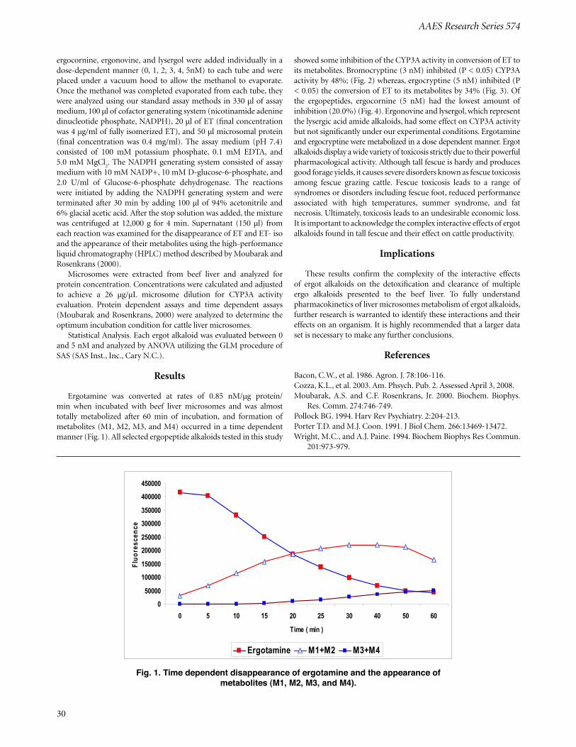


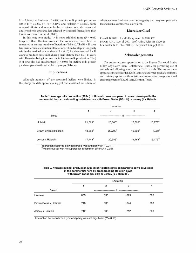


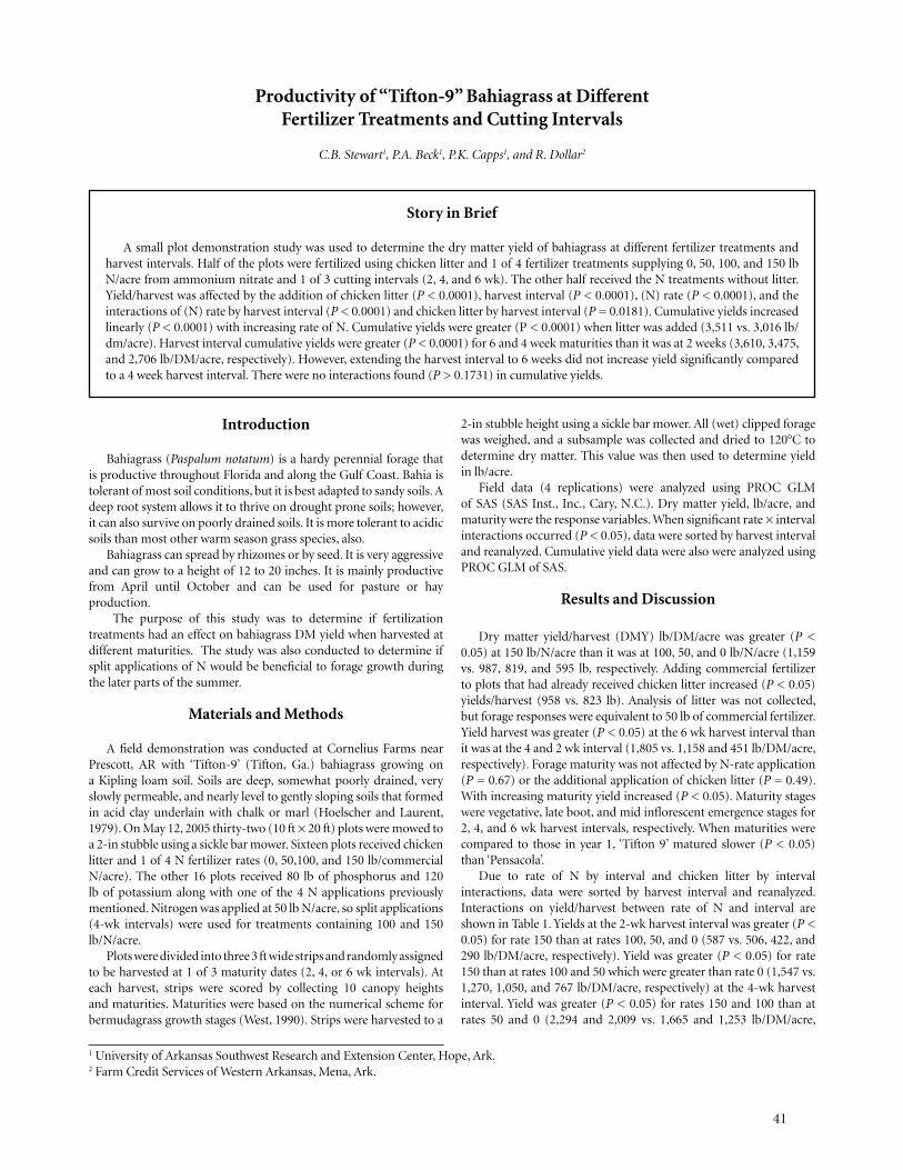


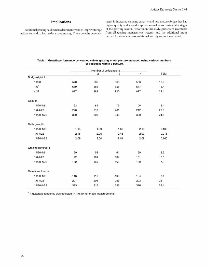


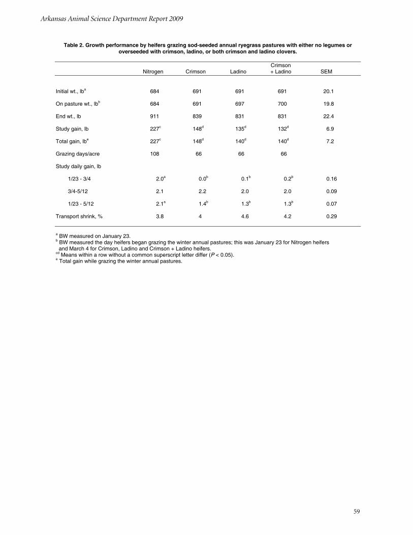


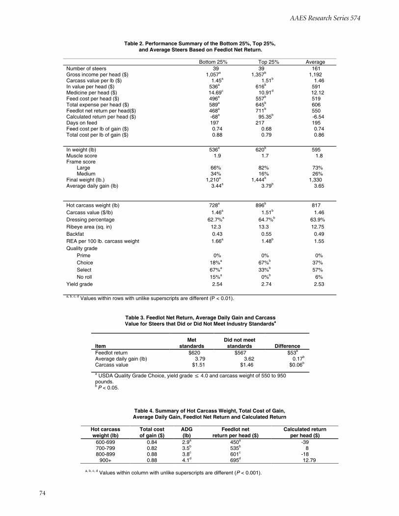


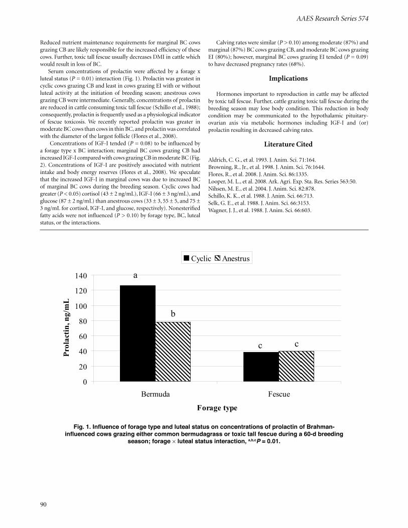


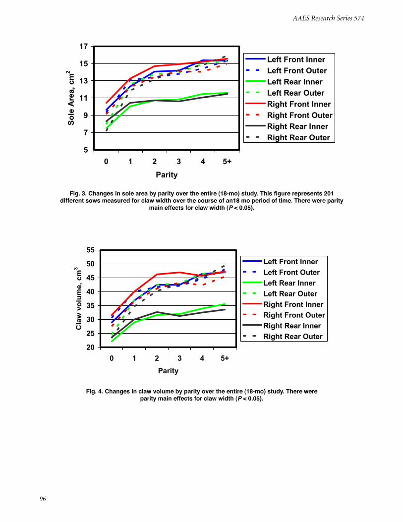

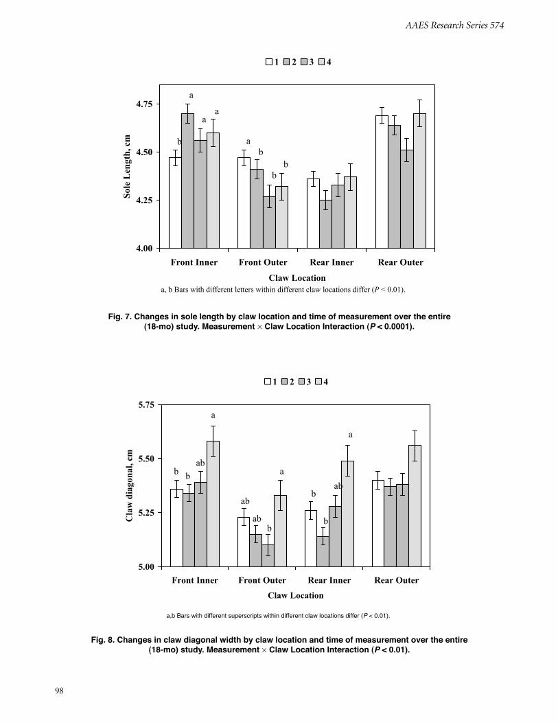
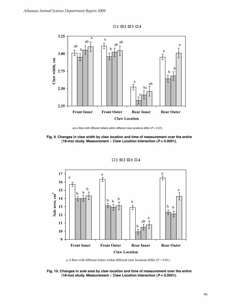

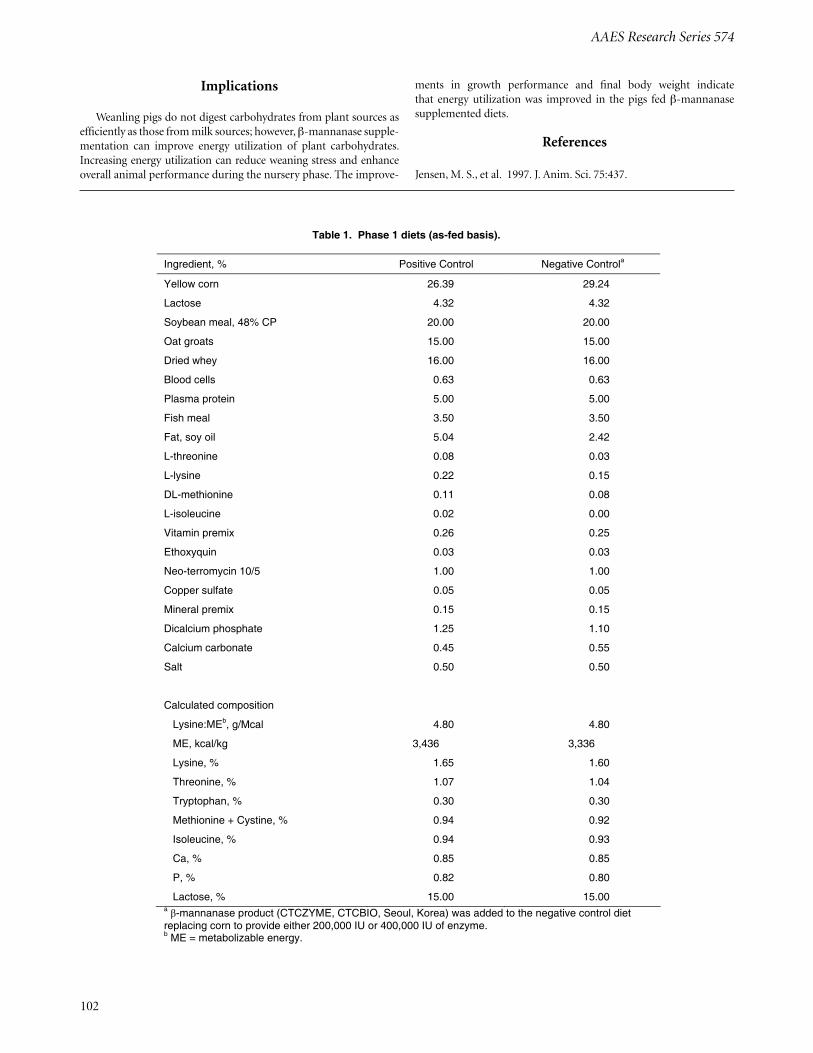


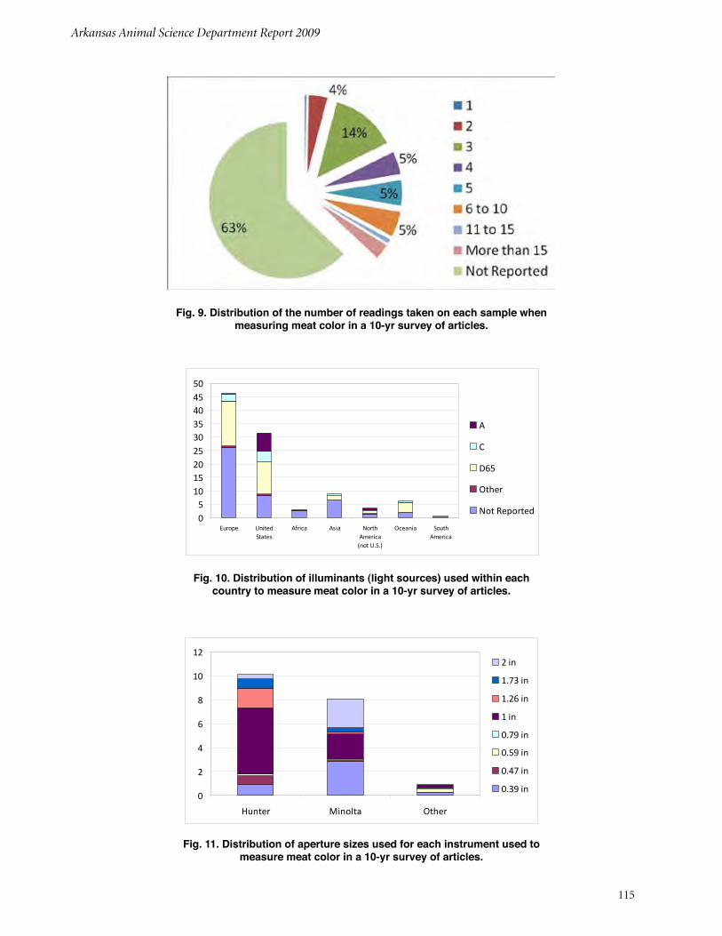


![Journal of the Arkansas Academy of Science · Journal of the Arkansas Academy of Science, Vol. 49 [1995], Art. 31 Published by Arkansas Academy of Science, 1995. 144 Supplies and](https://static.documents.pub/doc/80x56/5e36896471f98935c7381c67/journal-of-the-arkansas-academy-of-science-journal-of-the-arkansas-academy-of-science.jpg)


