46
Arquitectura de Sistemas Paralelos e Distribuídos Paulo Marques Dep. Eng. Informática – Universidade de Coimbra [email protected] Ago/2007 3. Programming Models
| Date post: | 21-Dec-2015 |
| Category: |
Documents |
| View: | 224 times |
| Download: | 0 times |

Arquitectura de Sistemas Paralelos e Distribuídos
Paulo MarquesDep. Eng. Informática – Universidade de [email protected]
Ago
/200
7
3. Programming Models
2
So, how do I program these things?
3
The main programming models…
A programming model abstracts the programmer from the hardware implementation
The programmer sees the whole machine as a big virtual computer which runs several tasks at the same time
The main models in current use are: Shared Memory Message Passing Data parallel / Parallel Programming Languages
Note that this classification is not all inclusive. There are hybrid approaches and some of the models overlap (e.g. data parallel with shared memory/message passing)

4
Shared Memory Model
Processor Thread
A
Processor Thread
B
Processor Thread
C
Processor Thread
D
double matrix_A[N];
double matrix_B[N];
double result[N];
Globally Accessible Memory (Shared)
5
Shared Memory Model
Independently of the hardware, each program sees a global address space
Several tasks execute at the same time and read and write from/to the same virtual memory
Locks and semaphores may be used to control access to the shared memory
An advantage of this model is that there is no notion of data “ownership”. Thus, there is no need to explicitly specify the communication of data between tasks.
Program development can often be simplified An important disadvantage is that it becomes more
difficult to understand and manage data locality. Performance can be seriously affected.

6
Shared Memory Modes
There are two major shared memory models: All tasks have access to all the address space
(typical in UMA machines running several threads) Each task has its address space. Most of the address
space is private. A certain zone is visible across all tasks. (typical in DSM machines running different processes)
(all the tasks sharethe same address space)
MemoryB
Shared memory
Memory
(all the tasks sharethe same address space)
MemoryA
A B C A B
MemoryB
Shared memory
7
Shared Memory Model –Closely Coupled Implementations
On shared memory platforms, the compiler translates user program variables into global memory addresses
Typically a thread model is used for developing the applications POSIX Threads OpenMP
There are also some parallel programming languages that offer a global memory model, although data and tasks are distributed
For DSM machines, no standard exists, although there are some proprietary implementations
8
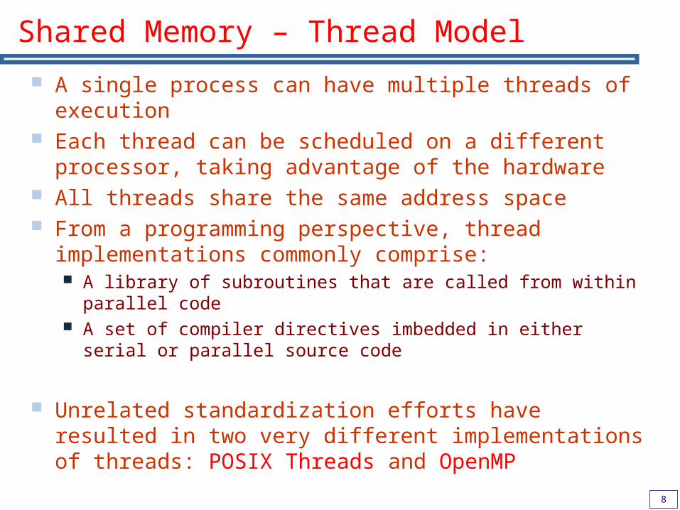
Shared Memory – Thread Model
A single process can have multiple threads of execution
Each thread can be scheduled on a different processor, taking advantage of the hardware
All threads share the same address space From a programming perspective, thread
implementations commonly comprise: A library of subroutines that are called from within parallel
code A set of compiler directives imbedded in either serial or
parallel source code
Unrelated standardization efforts have resulted in two very different implementations of threads: POSIX Threads and OpenMP
9
POSIX Threads
Library based; requires parallel coding Specified by the IEEE POSIX 1003.1c standard
(1995), also known as PThreads C Language Most hardware vendors / Operating Systems now
offer PThreads Very explicit parallelism; requires significant
programmer attention to detail

10
OpenMP
Compiler directive based; can use serial code Jointly defined and endorsed by a group of major
computer hardware and software vendors. The OpenMP Fortran API was released October 28, 1997. The C/C++ API was released in late 1998
Portable / multi-platform, including Unix and Windows NT platforms
Available in C/C++ and Fortran implementations Can be very easy and simple to use - provides for
“incremental parallelism” No free compilers available
11
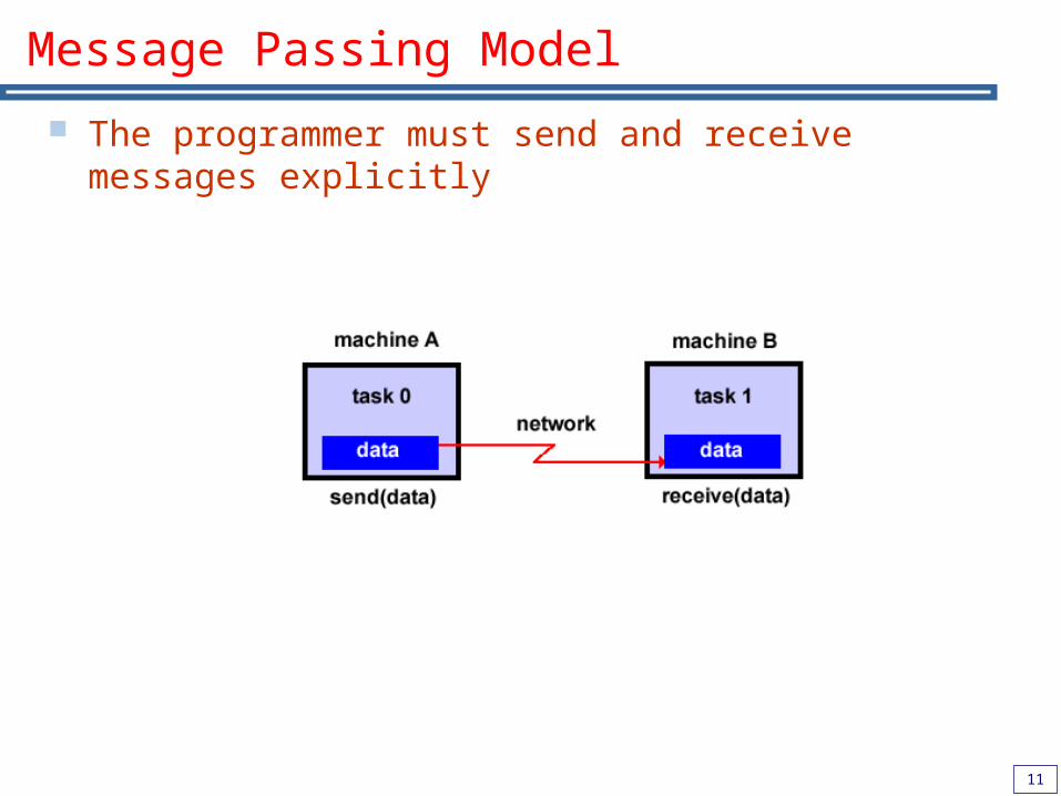
Message Passing Model
The programmer must send and receive messages explicitly
12
Message Passing Model
A set of tasks that use their own local memory during computation.
Tasks exchange data through communications by sending and receiving messages Multiple tasks can reside on the same physical machine as
well as across an arbitrary number of machines. Data transfer usually requires cooperative
operations to be performed by each process. For example, a send operation must have a matching receive operation.
13
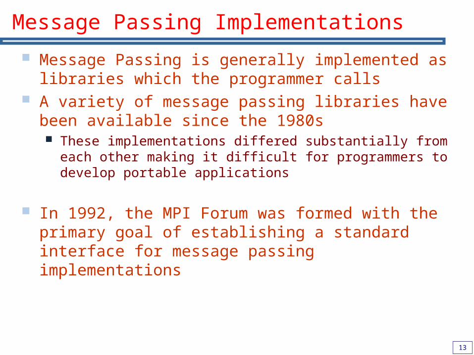
Message Passing Implementations
Message Passing is generally implemented as libraries which the programmer calls
A variety of message passing libraries have been available since the 1980s These implementations differed substantially from each
other making it difficult for programmers to develop portable applications
In 1992, the MPI Forum was formed with the primary goal of establishing a standard interface for message passing implementations
14
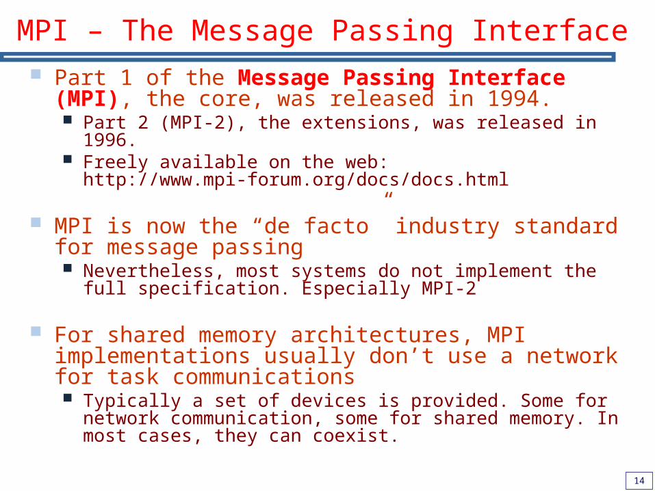
MPI – The Message Passing Interface Part 1 of the Message Passing Interface (MPI),
the core, was released in 1994. Part 2 (MPI-2), the extensions, was released in 1996. Freely available on the web:
http://www.mpi-forum.org/docs/docs.html
MPI is now the “de facto” industry standard for message passing Nevertheless, most systems do not implement the full
specification. Especially MPI-2
For shared memory architectures, MPI implementations usually don’t use a network for task communications Typically a set of devices is provided. Some for network
communication, some for shared memory. In most cases, they can coexist.
15
Data Parallel Model
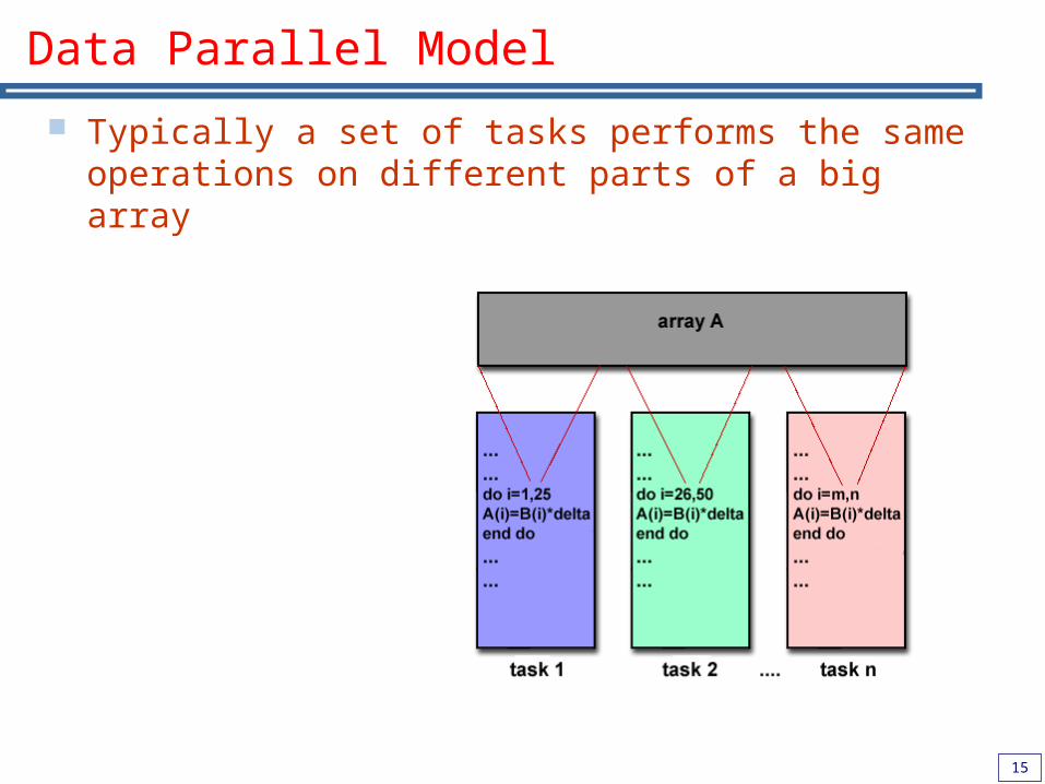
Typically a set of tasks performs the same operations on different parts of a big array

16
Data Parallel Model The data parallel model demonstrates the
following characteristics: Most of the parallel work focuses on performing
operations on a data set The data set is organized into a common structure, such
as an array or cube A set of tasks works collectively on the same data
structure, however, each task works on a different partition of the same data structure
Tasks perform the same operation on their partition of work, for example, “add 4 to every array element”
On shared memory architectures, all tasks may have access to the data structure through global memory.
On distributed memory architectures the data structure is split up and resides as "chunks" in the local memory of each task
17
Data Parallel Programming Typically accomplished by writing a program with
data parallel constructs calls to a data parallel subroutine library compiler directives
In most cases, parallel compilers are used: High Performance Fortran (HPF):
Extensions to Fortran 90 to support data parallel programming
Compiler Directives: Allow the programmer to specify the distribution and alignment of data. Fortran implementations are available for most common parallel platforms
DM implementations have the compiler convert the program into calls to a message passing library to distribute the data to all the processes. All message passing is done invisibly to the programmer

18
Summary
Middleware for parallel programming: Shared memory: all the tasks (threads or processes) see a
global address space. They read and write directly from memory and synchronize explicitly.
Message passing: the tasks have private memory. For exchanging information, they send and receive data through a network. There is always a send() and receive() primitive.
Data parallel: the tasks work on different parts of a big array. Typically accomplished by using a parallel compiler which allows data distribution to be specified.
Arquitectura de Sistemas Paralelos e Distribuídos
Paulo MarquesDep. Eng. Informática – Universidade de [email protected]
Ago
/200
7
Dividing up the Work

20
Decomposition – Idea
One of the first steps in designing a parallel program is to break the problem into discrete “chunks” of work that can be distributed to multiple tasks Decomposition or Partitioning
for (int i=0; i<N; i++) { heavy_stuff(i);}
Serial Programfor (int i=0; i<=N/2; i++) { heavy_stuff(i);}
for (int i=N/2+1; i<N; i++) { heavy_stuff(i);}
Task 0
Task 1
Parallel Program

21
Decomposition
In practice, the source code and executable is the same for all processes So, how do I get
asymmetry?
There’s always a primitive that returns the number of the process, and one that returns the size of the world (total processes): whoami() totalprocesses()
…
int main() { int lower, upper;
if (whoami() == 0) { lower = 0; higher = N/2+1; } else { lower = N/2 + 1; higher = N; }
for (int i=lower; i<higher; i++) { heavy_stuff(i);}

22
Decomposition Models
Decomposition
Trivial Functional Data
Balanced Unbalanced
23
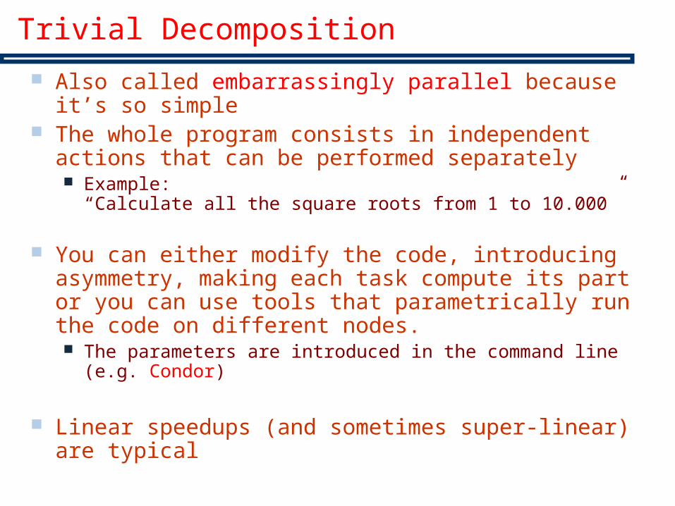
Trivial Decomposition
Also called embarrassingly parallel because it’s so simple
The whole program consists in independent actions that can be performed separately Example:
“Calculate all the square roots from 1 to 10.000”
You can either modify the code, introducing asymmetry, making each task compute its part or you can use tools that parametrically run the code on different nodes. The parameters are introduced in the command line (e.g.
Condor)
Linear speedups (and sometimes super-linear) are typical
24
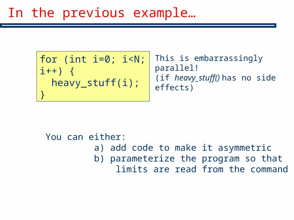
In the previous example…
for (int i=0; i<N; i++) { heavy_stuff(i);}
You can either: a) add code to make it asymmetric b) parameterize the program so that limits are read from the command line
This is embarrassingly parallel!(if heavy_stuff() has no side effects)

25
Functional Decomposition
The focus is on the computation that is to be performed rather than on the data manipulated by the computation
The problem is decomposed according to the work that must be done. Each task then performs a portion of the overall work.

26
Functional Decomposition - Pipelining
A simple form of functional decomposition is Pipelining
Each input passes through each of the subprograms in a given order.
Parallelism is introduced by having several inputs moving through the pipeline simultaneously
For an n-depth pipeline, an n speedup is theoretically possible
It depends on the slowest step of the pipeline
Input Image
Smoothing FilteringFeature
RecognitionSave
27
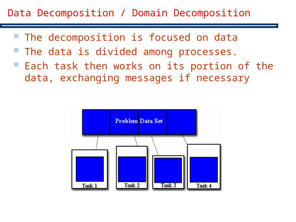
Data Decomposition / Domain Decomposition
The decomposition is focused on data The data is divided among processes. Each task then works on its portion of the data,
exchanging messages if necessary

28
Regular and Non-regular Decomposition
Non-Regular
Regular
Regular

29
Why not always use regular?
Different parts of the domain may take very different times to calculate/simulate
30
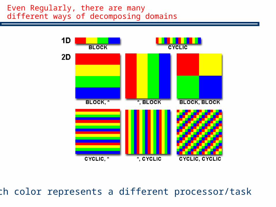
Even Regularly, there are many different ways of decomposing domains
Each color represents a different processor/task

31
Matrix Multiplication
double A[N][N], B[N][N], C[N][N];
for (int i=0; i<N; i++) { for (int j=0; j<N; j++) { C[i][j] = 0.0; for (int k=0; k<N; k++) C[i][j] += A[i][k]*B[k][j]; }}
As you can see, in matrix multiplication, all the results inC[N][N] are independent of each other!

32
Quiz – Matrix Multiplication
How should the task of computing matrix C be divided among 4 processors? Assume you are using a shared memory model, matrixes
A and B are copied to local memory. C is globally shared. The used language: C/C++
Implications on a UMA, NUMA and DSM machine
Matrix C

33
Data Decomposition
When considering data decomposition, two different types of execution models are typical: task farming and step lock execution (in grid)
In Task Farming, there is a master that sends out jobs which are processed by workers. The workers send back the results.
In Step Lock Execution, there is a data grid in which a certain operation is performed on each point. The grid is divided among the tasks. In each iteration, a new value of each data point is calculated

34
Example of Task Farming
Mandelbrot Set There is a complex plane
with a certain number of points.
For each point C, the following formula is calculated: z←z2+C, where z is initially 0.
If after a certain number of iterations, |z|>=4, the sequence is divergent, and it is colored in a way that represents how fast it is going towards infinity
If |z|<4, it will eventually converge to 0, so it is colored black
1 + 1.6i-2.3 + 1.6i
-2.3 - 1.6i 1 - 1.6i

35
Task Farming Mandelbrot(DSM – Message Passing Model)
Each worker asks the master for a job
The master sees what there is still to be processed, and sends it to the worker
The worker performs the job, and sends the result back to the master, asking it for another job MASTER
WORKER1
WORKER2
WORKERN
-2.3 + 1.6i 1 + 1.6i
-2.3 - 1.6i 1 - 1.6i
36
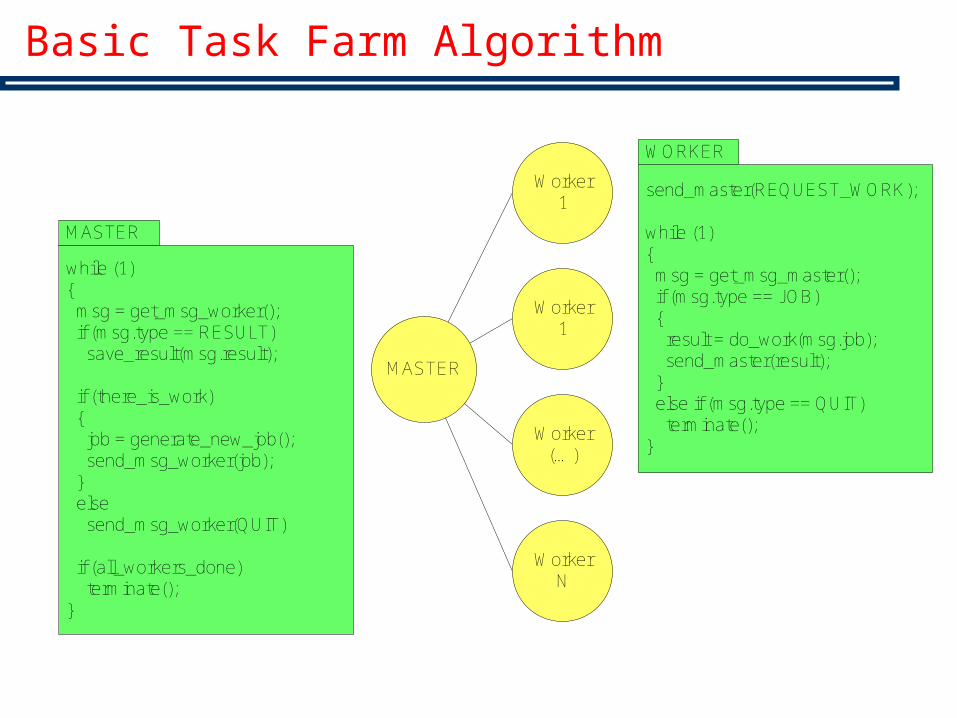
Basic Task Farm Algorithm
MASTER
Worker1
Worker1
Worker(…)
WorkerN
send_master(REQUEST_WORK);
while (1){ msg = get_msg_master(); if (msg.type == JOB) { result = do_work(msg.job); send_master(result); } else if (msg.type == QUIT) terminate();}
WORKER
while (1){ msg = get_msg_worker(); if (msg.type == RESULT) save_result(msg.result);
if (there_is_work) { job = generate_new_job(); send_msg_worker(job); } else send_msg_worker(QUIT)
if (all_workers_done) terminate();}
MASTER
37
Improved Task Farming
With the basic task farm, workers are idle while waiting for another task
We can increase the throughput of the farm by buffering tasks on workers
Initially the master sends workers two tasks: one is buffered and the other is worked on
Upon completion, a worker sends the result to the master and immediately starts working on the buffered task
A new task received from the master is put into the buffer by the worker
Normally, this requires a multi-threaded implementation
Sometimes it is advisable to have an extra process, called sink, where the results are sent to
38
Load Balancing Task Farms
Workers request tasks from the source when they require more work, i.e. task farms are intrinsically load balanced
Also, load balancing is dynamic, i.e., tasks are assigned to workers as they become free. They are not allocated in advance
The problem is ensuring all workers finish at the same time
Also, for all this to be true, the granularity of the tasks must be adequate Large tasks Poor load balancing Small tasks Too much communication
39
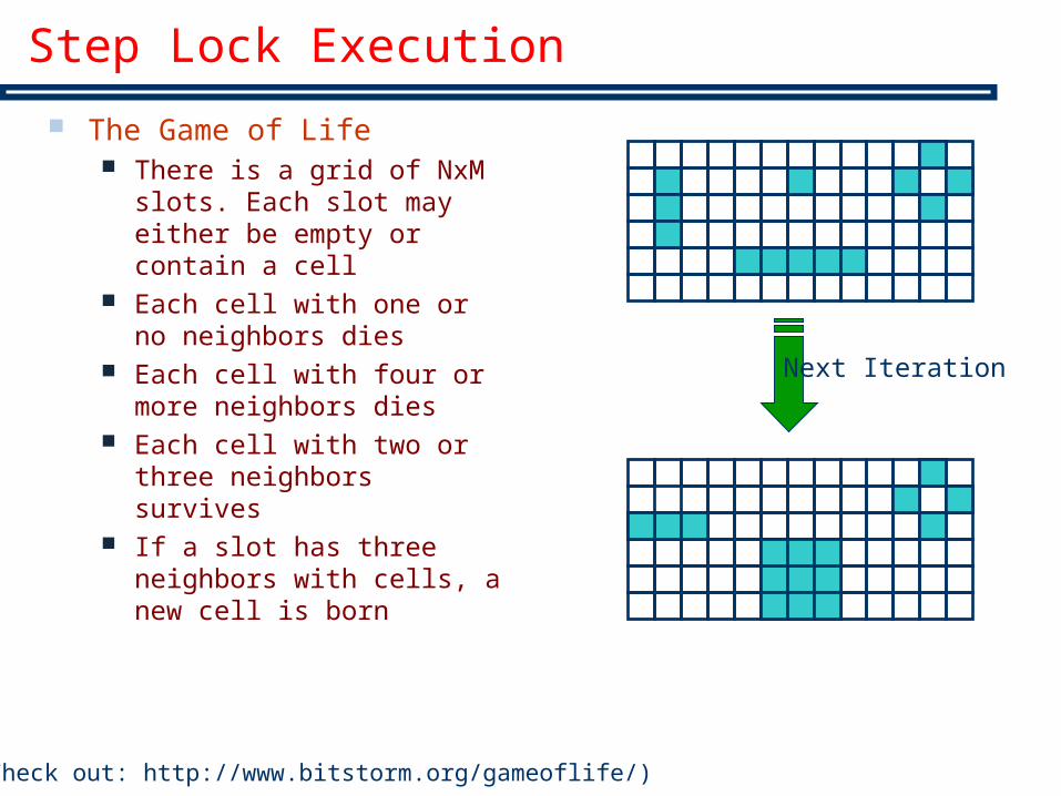
Step Lock Execution
The Game of Life There is a grid of NxM slots.
Each slot may either be empty or contain a cell
Each cell with one or no neighbors dies
Each cell with four or more neighbors dies
Each cell with two or three neighbors survives
If a slot has three neighbors with cells, a new cell is born
(Check out: http://www.bitstorm.org/gameoflife/)
Next Iteration
40
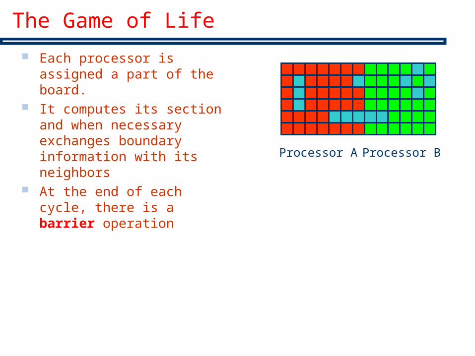
The Game of Life
Each processor is assigned a part of the board.
It computes its section and when necessary exchanges boundary information with its neighbors
At the end of each cycle, there is a barrier operation
Processor A Processor B

41
The Game of Life
On a Shared Memory Architecture Quite simple, just compute the assigned slots and perform
a barrier at the end of the cycle
On a DM Architecture / Message Passing Send the boundary information to the adjacent processors Collect boundary information from the adjacent
processors Compute the next iteration
Processor A Processor B

42
Step Lock Execution on Grids
When decomposing a domain, the grids must not be equal. But they must take approximately the same time to compute It’s a question of load balancing
At each iteration, a process is responsible for updating its local section of the global data block. Two types of data are involved: Local data which the process is responsible for updating Data which other processors are responsible for updating

43
Boundary Swapping
As seen in the game of life, each process owns a halo of data elements shadowed from neighboring processes
At each iteration, processes send copies of their edge regions to adjacent processes to keep their halo regions up to date This is known as
boundary swapping
Processor 1 Processor 2
Processor 3 Processor 4
update with internal information
update with informationfrom a neighbor processor

44
Boundary Conditions
Boundary swaps at edges of the global grid need to take into account the boundary conditions of the global grid
Two common types of boundary conditions Periodic boundaries Finite (or static) boundaries
Neighbors Target cell
Finite Boundary Periodic Boundary

45
Final Considerations…
Beware of Amdahl's Law!
46
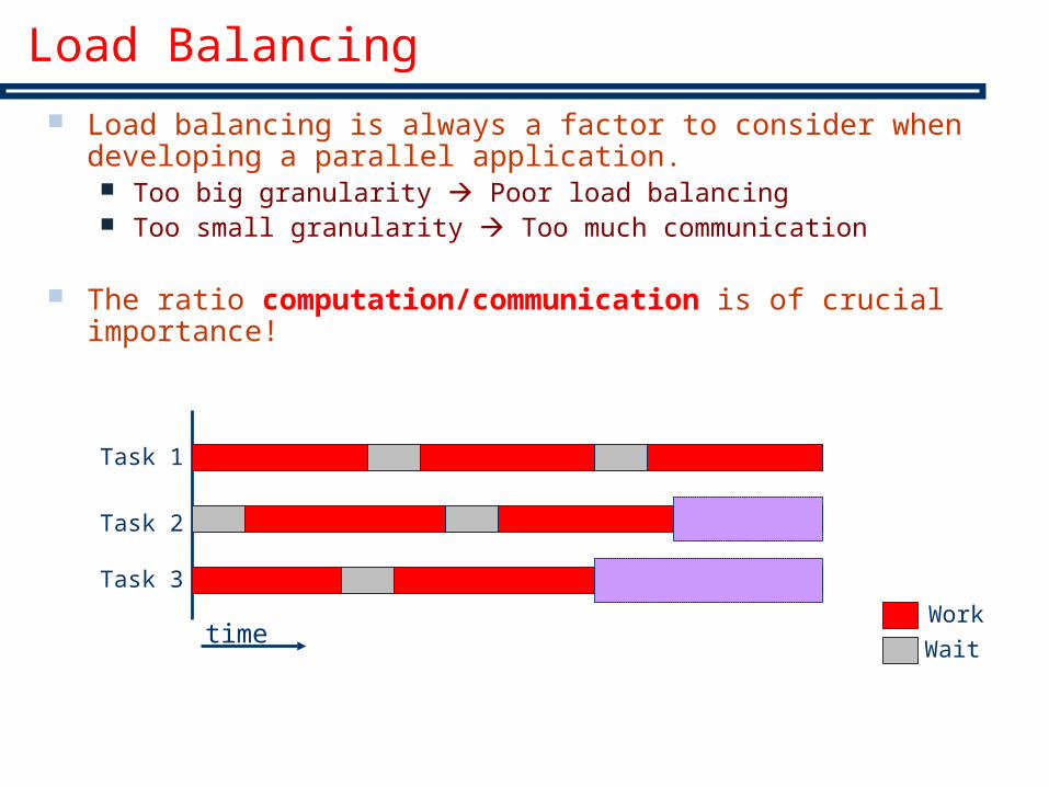
Load Balancing
Load balancing is always a factor to consider when developing a parallel application. Too big granularity Poor load balancing Too small granularity Too much communication
The ratio computation/communication is of crucial importance!
timeWork
Wait
Task 1
Task 2
Task 3


