Array Processing and Precoding Design for Next Generation ...

UNIVERSIDADE FEDERAL DO CEARA

CENTRO DE TECNOLOGIA

DEPARTAMENTO DE ENGENHARIA DE TELEINFORMATICA

PROGRAMA DE POS-GRADUACAO EM ENGENHARIA DE TELEINFORMATICA

FAZAL-E-ASIM

ARRAY PROCESSING AND PRECODING DESIGN FOR NEXT GENERATION OF

WIRELESS COMMUNICATION SYSTEMS

FORTALEZA

2020

FAZAL-E-ASIM



Tese apresentada ao Curso de Doutoradoem Engenharia de Teleinformatica do Pro-grama de Pos-Graduacao em Engenharia deTeleinformatica do Centro de Tecnologia daUniversidade Federal do Ceara, como requisitoparcial a obtencao do tıtulo de doutor em Engen-haria de Teleinformatica. Area de Concentracao:Sinais e Sistemas

Orientador: Prof. Dr. techn. Dr. h. c. Josef A. NossekCoorientador: Prof. Dr. Charles Casimiro Cavalcante

FORTALEZA

2020

Dados Internacionais de Catalogação na Publicação Universidade Federal do Ceará

Biblioteca UniversitáriaGerada automaticamente pelo módulo Catalog, mediante os dados fornecidos pelo(a) autor(a)

A857a Asim, Fazal-E-. Array Processing and Precoding Design for Next Generation of Wireless Communication Systems /Fazal-E- Asim. – 2020. 118 f. : il. color.

Tese (doutorado) – Universidade Federal do Ceará, Centro de Tecnologia, Programa de Pós-Graduaçãoem Engenharia de Teleinformática, Fortaleza, 2020. Orientação: Prof. Dr. techn. Dr. h. c. Josef A. Nossek. Coorientação: Prof. Dr. Charles Casimiro Cavalcante.

1. Processamento de Sinais. 2. Comunicações Sem-Fio. 3. Estimação de parâmetros do Canal. 4. Ondasmilimétricas. 5. Beamforming. I. Título. CDD 621.38

FAZAL-E-ASIM



Thesis defended at the TeleinformaticsEngineering Doctorate Program at theTeleinformatics Engineering Post-GraduateProgram of the Technology Center at theFederal University of Ceara, as a requirementto obtain the doctor degree in TeleinformaticsEngineering. Concentration Area: Signalsand Systems.

Approved on: October 07 , 2020

EXAMINING COMMITTEE

Prof. Dr. techn. Dr. h. c. Josef A. Nossek(Advisor)

Universidade Federal do Ceara, Brazil/Technical University of Munich, Germany.

Prof. Dr. Charles Casimiro Cavalcante(Co-Advisor)

Universidade Federal do Ceara, Brazil.

Univ.-Prof. Dr.-Ing. Martin HaardtTechnische Universitat Ilmenau, Germany.

Univ.-Prof. Dr. Didier Le RuyetConservatoire National des Arts et Metiers,

France.

Prof. Dr.-Ing. Felix AntreichInstituto Tecnologico de Aeronautica, Brazil.

Prof. Dr. Andre Lima Ferrer de AlmeidaUniversidade Federal do Ceara, Brazil.

To my parents, family and friends.

ACKNOWLEDGEMENTS

This study was financed in part by the Coordenacao de Aperfeicoamento de Pessoal de Nıvel Supe-

rior - Brasil (CAPES) - Finance Code 001 and CNPq (Procs. 309472/2017-2 and 306616/2016-5).

I would like to thank my advisors, Prof. Dr. techn. Dr. h. c. Josef A. Nossek and Prof. Dr.

Charles Casimiro Cavalcante for their technical support at every stage of my Ph.D. In short, it

would not be possible without their support.

I am also very grateful to Prof. Dr. Andre Lima Ferrer de Almeida and Prof. Dr.-Ing. Felix

Antreich for sharing their knowledge and having technical discussions. I am also thankful to

Prof. Dr. Tarcisio Ferreira Maciel for his support and discussions during my stay at Wireless

Telecommunication Research Group (GTEL).

I would also like to thank all my GTEL colleagues especially, Dr. Igor Moaco Guerreiro, Dr.

Lucas Nogueira Ribeiro, Dr. Roberto Pinto Antonioli, Raphael Braga Evangelista, and Bruno

Sokal. To the last, but not least, I am thankful to my colleague and friend Alexandre Matos

Pessoa for the technical support and fruitful discussions. Finally, my special thanks to my parents

and family, who have been with me all the time.

RESUMO

A proxima geracao de sistemas de comunicacao sem fio promete fornecer uma melhor experiencia

do usuario em termos de altas taxas de dados, cobertura, confiabilidade e eficiencia energetica.

Uma das solucoes candidatas e a combinacao viavel de ondas milimetricas (mmWave) com

a introducao de um grande numero de antenas. Por um lado, o uso de mmWave facilitara a

implantacao de um grande numero de antenas, mas do outro lado vai impor um desafio de

implementacao de hardware com eficiencia energetica. Portanto, alem da eficiencia espectral,

a eficiencia energetica sera um importante objetivo de design. A introducao de um grande

numero de antenas na estacao base (BS) tambem complica a estimativa do parametro do canal.

A estimativa do parametro do canal deve ser obtida com alta resolucao no equipamento do

usuario (UE), pois esses parametros precisam ser quantizados antes de ser enviado de volta a BS

para pre-codificacao. Se os parametros do canal nao forem estimados com alta precisao, a BS

recebera os parametros errados com erros de quantizacao adicionais, resultando na deterioracao

do desempenho. Esta tese apresenta uma solucao de eficiencia energetica para superar o de-

safio de implementacao de hardware devido a introducao de um grande numero de antenas

atraves da introducao da matriz de Butler (BM) no domınio analogico usando a abordagem

de deslocamentos de fase analogicos parcialmente conectado (PCAPS). A implantacao da BM

melhora a implementacao do hardware mas torna a estimativa dos parametros do canal e a pre-

codificacao hıbrida mais desafiadores. Para atender a esses problemas, o estimador de maxima

verossimilhanca (ML) e inicialmente derivado para canais com desvanecimento de frequencia

plano, enquanto uma abordagem de dois estagios e projetada para estimativa de parametro

unidimensional assumindo canais seletivos em frequencia. A primeira etapa e realizada pela

proposicao da estimacao de parametros baseada em um algoritmo de grade DFT (PREIDG) para

encontrar as estimativas grosseiras, que e usado para inicializar o algoritmo de maximizacao

de expectativa generalizada alternada de espaco (SAGE) para obter estimativas dos parametros

atraves da ML. Alem disso, o problema e estendido a estimativa bidimensional de parametros,

que e resolvida pelo algoritmo de dois estagios. No primeiro estagio, um PREIDG modificado

e proposto para realizar uma estimativa grosseira que e usada para obter as estimativas de alta

resolucao dos parametros usando o algoritmo SAGE no segundo estagio. O desempenho dos

algoritmos de estimativa dos parametros sao avaliados derivando o limite inferior de Cramer-Rao

(CRLB). Finalmente, o algoritmo analogico e de banda base e obtido usando o metodo do erro

quadratico mınimo ponderado medio (WMMSE) de formacao de feixe hıbrido (HBF).

Palavras-chave: Beamforming. 5G. MIMO massivo. Ondas milimetricas. Estimacao de

parametros do Canal. Pre-codificacao analogica e de banda base.

ABSTRACT

The next generation of wireless communication systems promises to provide a better user experi-

ence in terms of high data rates, coverage, reliability, and energy efficiency. One of the competing

candidates is the viable combination of millimeter-wave (mmWave) with the introduction of a

large number of antennas. On one side, the use of mmWave will facilitate the deployment of

a large number of antennas but on the other side will impose a challenge of energy-efficient

hardware implementation. Therefore, in addition to spectral efficiency, energy efficiency will

be an important design goal. Introducing a large number of antennas at the base station (BS)

will also complicate the channel parameter estimation. The channel parameter estimation must

be obtained with high-resolution at the user equipment (UE), because these parameters need to

be quantized before being sent back to the BS for precoding. If the channel parameters are not

estimated with high accuracy, the BS will receive the erroneous parameters with additional quan-

tization errors, resulting in deterioration of performance. This thesis presents an energy-efficient

solution to overcome the challenge of hardware implementation due to the introduction of a large

number of antennas by introducing Butler matrix (BM) in the analog domain using partially

connected analog phase shifting (PCAPS) approach. The deployment of BM improves the hard-

ware implementation but makes the channel parameter estimation and hybrid precoding more

challenging. To cater to these problems, maximum likelihood (ML) estimator is initially derived

for frequency flat fading channels, while a two-stage approach is designed for one-dimensional

parameter estimation assuming frequency selective channels. The first stage is accomplished

by proposing parameter estimation based on a DFT grid (PREIDG) algorithm to find the coarse

estimates, which is used to initialize the space alternating generalized expectation-maximization

(SAGE) algorithm to get ML estimates of the parameters. Furthermore, the problem is extended

to two-dimensional parameter estimation, which is solved by the two-stage algorithm. In the first

stage a modified PREIDG is proposed to perform coarse estimation which is used to obtain the

high-resolution estimates of the parameters using the SAGE algorithm in the second stage. The

performance of the parameters estimation algorithms is assessed by deriving Cramer-Rao lower

bound (CRLB). Finally, the analog and baseband algorithm is obtained using hybrid beamforming

(HBF)-weighted minimum mean square error (WMMSE) method.

Keywords: Beamforming. 5G. Massive MIMO. Millimeter Wave. Channel Parameter Estima-

tion. Analog and Baseband Precoding.

LIST OF FIGURES

Figure 2.1 – Fully connected analog phase shifting network. . . . . . . . . . . . . . . . . 24

Figure 2.2 – Partially connected analog phase shifting network. . . . . . . . . . . . . . . 25

Figure 2.3 – Partially connected Butler matrix approach. . . . . . . . . . . . . . . . . . 26

Figure 2.4 – 90◦ hybrid coupler. . . . . . . . . . . . . . . . . . . . . . . . . . . . . . . 26

Figure 2.5 – A M ×M BM with M2

log2M , 90◦ hybrids and fixed phase shifters (PSs)

only, where w = exp(−j 2πM

) for M = 8. . . . . . . . . . . . . . . . . . . . 27

Figure 2.6 – Performance comparison of the proposed ML estimator with auxiliary beam

pair (ABP) method for angle of departure (AoD) θ estimation assuming line-

of-sight (LOS) path only. . . . . . . . . . . . . . . . . . . . . . . . . . . . 32

Figure 2.7 – Performance comparison the proposed ML estimator with ABP method for

AoD ˆ(√PTα) estimation assuming LOS path only. . . . . . . . . . . . . . . 33

Figure 2.8 – An example of integer delay estimation τi using power matrix P as in (2.37)

where p1 and p3 are the two diagonals, for which (2.39) is fulfilled. . . . . . 37

Figure 2.9 – An example of coarse estimation using discrete Fourier transform (DFT)

matrix based beamforming. . . . . . . . . . . . . . . . . . . . . . . . . . . 38

Figure 2.10–A flowchart for the two-stage estimation algorithm. . . . . . . . . . . . . . 42

Figure 2.11–Histogram for the number of iterations of SAGE in the two-stage algorithm. 45

Figure 2.12–Performance comparison of two-stage and ABP algorithm for LOS AoD,

assuming R = 3. . . . . . . . . . . . . . . . . . . . . . . . . . . . . . . . . 46

Figure 2.13–Performance comparison of two-stage and ABP algorithm for non-line-of-

sight (NLOS) AoD, assuming R = 3. . . . . . . . . . . . . . . . . . . . . . 47

Figure 2.14–Performance comparison of two-stage and ABP algorithm for αr. . . . . . . 47

Figure 2.15–Performance comparison of two-stage algorithm for τr . . . . . . . . . . . . 48

Figure 3.1 – An architecture of Butler matrices (BMs) exciting two-dimensional uniform

rectangular array. . . . . . . . . . . . . . . . . . . . . . . . . . . . . . . . 50

Figure 3.2 – A 4-point DFT building block. . . . . . . . . . . . . . . . . . . . . . . . . 50

Figure 3.3 – A 4× 4 BM using 90◦ hybrid couplers. . . . . . . . . . . . . . . . . . . . . 51

Figure 3.4 – Uniform planar array in y-z-plane. . . . . . . . . . . . . . . . . . . . . . . 54

Figure 3.5 – Two-dimensional power-table P′r for estimation of spatial frequencies µr and

ψr. . . . . . . . . . . . . . . . . . . . . . . . . . . . . . . . . . . . . . . . 56

Figure 3.6 – An example for constructing received power matrix P considering a 4 × 4

uniform rectangular array (URA). . . . . . . . . . . . . . . . . . . . . . . . 58

Figure 3.7 – An example of two-dimensional coarse estimation via three two-dimensional

beamforming vectors for the UE at (φ = 35◦, θ = 95◦) . . . . . . . . . . . . 60

Figure 3.8 – Histogram for the number of iterations of SAGE in the two-stage algorithm. 67

Figure 3.9 – Performance comparison of two-stage and ABP algorithm for LOS AoD

azimuth, assuming R = 3. . . . . . . . . . . . . . . . . . . . . . . . . . . . 67

Figure 3.10–Performance comparison of two-stage and ABP algorithm for NLOS AoDs

azimuth, assuming R = 3. . . . . . . . . . . . . . . . . . . . . . . . . . . . 68

Figure 3.11–Performance comparison of two-stage and ABP algorithm for LOS AoD

elevation, assuming R = 3. . . . . . . . . . . . . . . . . . . . . . . . . . . 68

Figure 3.12–Performance comparison of two-stage and ABP algorithm for NLOS AoDs

elevation, assuming R = 3. . . . . . . . . . . . . . . . . . . . . . . . . . . 69

Figure 3.13–Performance comparison of two-stage and ABP algorithm for√PTαr. . . . 69

Figure 3.14–Performance comparison of two-stage algorithm for τr . . . . . . . . . . . . 70

Figure 4.1 – Average spectral efficiency of the proposed hybrid analog and digital precoder. 79

Figure 4.2 – Convergence of the HBF-WMMSE approach. . . . . . . . . . . . . . . . . 85

Figure 4.3 – Sum-rate performance comparison for different algorithms as compared to

HBF-WMMSE method for multiple-input single-output (MISO) system. . . 86

LIST OF TABLES

Table 2.1 – Beamforming angles using one 16× 16 BM . . . . . . . . . . . . . . . . . . 44

Table 3.1 – Beamforming angles using eight 4× 4 BMs . . . . . . . . . . . . . . . . . . 71

Table 3.2 – Beamforming angles using eight 8× 8 BMs . . . . . . . . . . . . . . . . . . 71

Table 3.3 – Remaining beamforming angles using eight 8× 8 BMs . . . . . . . . . . . . 73

LIST OF ABBREVIATIONS AND ACRONYMS

5G fifth-generation

ABP auxiliary beam pair

ADC analog/digital converter

AoA angle of arrival

AoD angle of departure

BC broadcast channel

BCD block coordinate descent

BM Butler matrix

BMs Butler matrices

bpcu bits per channel use

BS base station

CAZAC constant amplitude zero auto correlation

CRLB Cramer-Rao lower bound

CS compressive sensing

CSI channel state information

DFT discrete Fourier transform

EM Expectation-Maximization

ESPRIT estimation of signal parameters via rotational invariant techniques

FCAPS fully connected analog phase shifting

FFT fast Fourier transform

FIM Fisher information matrix

GoB grid of beams

HBF hybrid beamforming

IBC interference broadcast channel

JADE joint angle and delay estimation

KKT Karush-Kuhn-Tucker

LOS line-of-sight

LUT Look-up table

MF matched filter

MIMO multiple-input multiple-output

MISO multiple-input single-output

ML maximum likelihood

MMSE minimum mean square error

mmWave millimeter-wave

MSE mean square error

MU-MIMO multi-user MIMO

MU-MISO multi-user MISO

MUSIC multiple signal classification

NLOS non-line-of-sight

OMP orthogonal matching pursuit

PA power amplifier

PCAPS partially connected analog phase shifting

PCBM partially connected Butler matrix

PCBMS partially connected Butler matrices

pdf probability density function

PREIDG parameter estimation based on a DFT grid

PS phase shifter

PSs phase shifters

QPSK quadrature phase shift-keying

RC raised cosine

RF radio-frequency

RMSE root mean square error

SAGE space alternating generalized expectation-maximization

SFG signal-flow graph

SINR signal-to-interference and noise ratio

SNR signal-to-noise ratio

SU-MISO single-user MISO

UE user equipment

ULA uniform linear array

URA uniform rectangular array

WMMSE weighted minimum mean square error

ZF zero forcing

NOTATION

imaginary unit√−1

a scalar

a vector

A matrix

R the real numbers field

C the complex numbers field

(·)∗ complex conjugate

(·)T transpose

(·)H conjugate transpose (Hermitian)

(·)−1 inverse operator

(·)† Moore-Penrose pseudo-inverse

‖ · ‖2 `2 norm

‖ · ‖F Frobenius norm

E [·] statistical expectation

| · | absolute value (complex magnitude)

b·c floor operation

⊗ Kronecker product

◦ outer product

� elementwise (Hadamard) product

� Khatri-Rao product

O(·) big-O notation

IN N -dimensional identity matrix

0M×N (M ×N)-dimensional null matrix

1M×N (M ×N)-dimensional all ones matrix

tr{·} matrix trace

det(·) matrix determinant

diag{·} transforms an input vector into a diagonal matrix

vec(·) vectorizes the input array

unvec(·) reshapes a column vector into a matrix

U(a, b) uniform distribution from a to b

CN (µ,Σ) complex Gaussian distribution with mean µ and covariance matrix Σ

[A]p,q entry of A at the pth row and qth column

max(a) gives the index of the maximum value in vector a

mod (·) modulus

CONTENTS

1 INTRODUCTION . . . . . . . . . . . . . . . . . . . . . . . . . . . . . . 19

1.1 Motivation . . . . . . . . . . . . . . . . . . . . . . . . . . . . . . . . . . . 19

1.2 Contributions and Thesis Organizations . . . . . . . . . . . . . . . . . . 21

1.2.1 Publications . . . . . . . . . . . . . . . . . . . . . . . . . . . . . . . . . . 22

2 ONE-DIMENSIONAL CHANNEL PARAMETER ESTIMATION . . . 24

2.1 Overview . . . . . . . . . . . . . . . . . . . . . . . . . . . . . . . . . . . 24

2.2 Contributions . . . . . . . . . . . . . . . . . . . . . . . . . . . . . . . . . 27

2.3 ML Estimation for Frequency Flat Fading Channel . . . . . . . . . . . . 28

2.3.1 System Model . . . . . . . . . . . . . . . . . . . . . . . . . . . . . . . . . 29

2.3.2 ML Estimation . . . . . . . . . . . . . . . . . . . . . . . . . . . . . . . . . 30

2.3.3 CRLB . . . . . . . . . . . . . . . . . . . . . . . . . . . . . . . . . . . . . 31

2.3.4 Numerical Results . . . . . . . . . . . . . . . . . . . . . . . . . . . . . . . 32

2.4 Two-stage Estimation Algorithm for Frequency Selective Fading Channel 34

2.4.1 System Model . . . . . . . . . . . . . . . . . . . . . . . . . . . . . . . . . 34

2.4.2 PREIDG based coarse estimation . . . . . . . . . . . . . . . . . . . . . . 35

2.4.3 ML Estimation Using SAGE . . . . . . . . . . . . . . . . . . . . . . . . . 40

2.4.4 CRLB . . . . . . . . . . . . . . . . . . . . . . . . . . . . . . . . . . . . . 42


3 TWO-DIMENSIONAL CHANNEL PARAMETER ESTIMATION . . . 49

3.1 Overview . . . . . . . . . . . . . . . . . . . . . . . . . . . . . . . . . . . 49

3.1.1 Construction of 4× 4 BM . . . . . . . . . . . . . . . . . . . . . . . . . . . 50

3.2 Contributions . . . . . . . . . . . . . . . . . . . . . . . . . . . . . . . . . 51

3.3 Two-Dimensional Parameter Estimation Algorithm for Frequency Selec-

tive Channel . . . . . . . . . . . . . . . . . . . . . . . . . . . . . . . . . . 52

3.3.1 System Model . . . . . . . . . . . . . . . . . . . . . . . . . . . . . . . . . 52

3.3.2 Coarse estimation based on modified PREIDG . . . . . . . . . . . . . . . 54

3.3.3 Look-up table (LUT) . . . . . . . . . . . . . . . . . . . . . . . . . . . . . 55

3.3.4 Estimation of Spatial Frequencies . . . . . . . . . . . . . . . . . . . . . . 56

3.3.5 Example with a 4× 4 URA . . . . . . . . . . . . . . . . . . . . . . . . . . 57

3.3.6 High-resolution channel parameter estimation using SAGE . . . . . . . . 60

3.3.7 Complexity of the proposed two-step approach . . . . . . . . . . . . . . . . 63

3.3.8 CRLB . . . . . . . . . . . . . . . . . . . . . . . . . . . . . . . . . . . . . 64


3.3.10 Exciting URA with 4× 4 and 8× 8 BMs . . . . . . . . . . . . . . . . . . . 69

4 ANALOG AND BASEBAND PRECODING . . . . . . . . . . . . . . . . 74

4.1 Overview . . . . . . . . . . . . . . . . . . . . . . . . . . . . . . . . . . . 74

4.2 Contributions . . . . . . . . . . . . . . . . . . . . . . . . . . . . . . . . . 74

4.3 Single-cell, single-user MISO (SU-MISO) . . . . . . . . . . . . . . . . . 75

4.3.1 System Model . . . . . . . . . . . . . . . . . . . . . . . . . . . . . . . . . 75

4.3.2 Analog Precoder Design . . . . . . . . . . . . . . . . . . . . . . . . . . . 76

4.3.3 Baseband Precoder design . . . . . . . . . . . . . . . . . . . . . . . . . . 77

4.3.4 Numerical result . . . . . . . . . . . . . . . . . . . . . . . . . . . . . . . . 78

4.4 Single-cell, multi-user MISO (MU-MISO) . . . . . . . . . . . . . . . . . 79

4.4.1 System Model . . . . . . . . . . . . . . . . . . . . . . . . . . . . . . . . . 79

4.4.2 Analog Precoder Design . . . . . . . . . . . . . . . . . . . . . . . . . . . 80

4.4.3 Baseband Precoder Design . . . . . . . . . . . . . . . . . . . . . . . . . . 81


5 CONCLUSION AND PERSPECTIVES . . . . . . . . . . . . . . . . . . 87

REFERENCES . . . . . . . . . . . . . . . . . . . . . . . . . . . . . . . . 89

APPENDICES . . . . . . . . . . . . . . . . . . . . . . . . . . . . . . . . 95

APPENDIX A – ML Estimation and CRLB . . . . . . . . . . . . . . . 96

A.1 Maximum Likelihood estimation for frequency flat fading channel . . . 96

A.2 Derivation of the Fisher information matrix (FIM) F(η) . . . . . . . . . 99

A.3 SAGE . . . . . . . . . . . . . . . . . . . . . . . . . . . . . . . . . . . . . 99

A.4 Derivation of the FIM F(η) . . . . . . . . . . . . . . . . . . . . . . . . . 107

APPENDIX B – High-Resolution Estimation using SAGE and CRLB 109

B.1 SAGE . . . . . . . . . . . . . . . . . . . . . . . . . . . . . . . . . . . . . 109

B.2 Derivation of the FIM F(η) . . . . . . . . . . . . . . . . . . . . . . . . . 112

APPENDIX C – Analog and Baseband Precoders . . . . . . . . . . . 114

C.1 Achievable sum-rate for single-cell multiuser . . . . . . . . . . . . . . . 114

C.2 mean square error (MSE) minimization for kth user . . . . . . . . . . . 115

C.3 HBF-WMMSE for MU-MISO . . . . . . . . . . . . . . . . . . . . . . . . 117

19

1 INTRODUCTION

1.1 Motivation

The next generation of wireless communication systems envisioned to support very

high data rates for the UEs. To turn this ambitious goal into reality, the use of high bandwidth is

essential, which is only possible by moving to the mmWave bands [1, 2]. The use of such higher

frequencies will facilitate the deployment of massive multiple-input multiple-output (MIMO) at

the BS to achieve high beamforming gains. The available large bandwidth combined with a large

number of antennas directly imposes challenges for hardware implementation of such a system

[3]. Consequently, in addition to spectral efficiency, energy efficiency becomes an important

design goal.

To combat this issue, multiple solutions are proposed to ensure the practicality of the

large antenna systems, as the use of one radio-frequency (RF) chain per antenna seems not to be

a feasible solution with high resolution analog/digital converter (ADC)s. One of the proposed

solutions is the use of low resolution ADC [4, 5, 6]. Another solution is to divide the full digital

beamforming into two parts, i.e., analog beamforming and digital baseband precoding [7, 8, 9, 10].

There are two main approaches of hybrid beamforming, namely fully connected analog phase

shifting (FCAPS) and partially connected analog phase shifting (PCAPS) network, both of which

have pros and cons. In both the strategies dividers are used which divide the signals form the

RF-chains to the multitude of PSs. Keep in mind, that the dividers are theoretical lossless, for

instance, Wilkinson splitter. The combiners are used only in FCAPS network, which combines

the signals from many PSs before the power amplifier (PA) of each antenna which introduces

losses. These losses are channel-dependent and depend on the mutual correlation of the precoded

signals, which can have a maximum loss of 3 dB, if the two signals are uncorrelated. Furthermore,

the total number of PSs required in FCAPS approach is more as compared to PCAPS network,

while the using FCAPS, we can form beams by using all the antennas simultaneously.

To cater to this energy losses and to ease the hardware complexity of so many PSs,

we introduced BM, which uses fixed PSs and can be constructed with a theoretical lossless

90◦ hybrid coupler [11, 12, 13]. A BM with low insertion loss is shown in [14]. A BM is

the analog implementation of the DFT matrix, which one side provides the energy-efficient

hardware implementation in the analog domain but on the other side makes the channel parameter

estimation and precoding more challenging.

Chapter 1. Introduction 20

The mmWave channel estimation becomes more challenging by the introduction of a

massive number of antennas at the BS due to its high dimensionality, and it can be even more

complicated by introducing the frequency selectivity [15, 16, 17]. Furthermore, the mmWave

range is characterized by the sparsity in the angular domain, which facilitates the design of

low-complexity compressive sensing (CS) based parameter estimation techniques. Recently,

many techniques have been studied for channel parameter estimation by exploiting the sparsity of

the channel [18, 19, 20, 21]. An adaptive codebook for channel parameter estimation via CS [22],

while an orthogonal matching pursuit (OMP) approach is used in [23] to estimate the channel

parameters. By introducing quantized PSs in [24], channel parameter estimation is achieved

using frequency selective channels. A two-stage algorithm is introduced in [25] for position

and orientation estimation. The authors in [26, 27] proposed a so called beam pairing approach,

where many beam pairs are formed, to calculate set of many ratios to estimate the corresponding

AoD and angle of arrival (AoA), respectively. The ABP method outperforms grid of beams

(GoB) method [28].

The authors in [29] proposed a super-resolution algorithm for flat-fading channels,

and further showed that the ABP method outperforms the standard CS techniques based on

adaptive codebook and OMP. The work in [30] proposed two high-resolution algorithms based

on estimation of signal parameters via rotational invariant techniques (ESPRIT), named as two-

dimensional ESPRIT and the minimum searching for frequency selective channels. However,

the algorithms are unable to show good performance in the low signal-to-noise ratio (SNR)

regime which is important for mmWave fifth-generation (5G) systems. Indeed, ESPRIT is more

sensitive to sensor location errors and mutual coupling because of the assumption of translational

invariance of subarray responses [31, 32]. However, the SAGE algorithm does not impose such

kind of restriction on the subarray responses and outperforms multiple signal classification

(MUSIC), ESPRIT and joint angle and delay estimation (JADE) algorithms [33, 34, 35, 36, 37].

Most of the aforementioned work are restricted to uniform linear array (ULA) and frequency flat

fading channels.

After the BS gets the estimates of the channel parameters, the next task is the optimal

precoding to maximize the spectral efficiency of the users and minimize the inter-user interference.

As mentioned earlier, one of the approaches is hybrid beamforming where analog beamforming

can be implemented using PSs [38], switches[39] and lenses [40]. The authors in [41] used an

alternating and manifold optimization based hybrid beamforming algorithm which put constraint

of constant modulus on the design of analog phase shifter (PS). Similarly, the work in [42]


assumes variable PSs in the design of analog and baseband precoding. The authors in [43]

analyses the energy efficiency of FCAPS and PCAPS assuming realistic RF modeling. The work

in [44], designed hybrid beamforming and combining strategies, wherein the first approach, the

combiners are designed separately, while the analog and baseband precoders are jointly optimized

by minimizing the system sum-MSE. In the latter, an iterative WMMSE algorithm is used to

jointly optimized both the analog and digital precoders/combiners.

1.2 Contributions and Thesis Organizations

This thesis focus on two very important problems, one is channel parameter estimation

and the other is analog RF and digital baseband precoding. As discussed earlier, to have an

energy-efficient hardware implementation, a BM is introduced to excite an ULA, which is the

analog implementation of a DFT matrix. A ML estimator is derived to achieve efficient channel

parameter estimates for frequency-flat fading channels. The same setup is extended for frequency-

selective channels, which makes it a multidimensional, non-linear optimization problem. To

achieve an ML estimates, a two-step estimation algorithm is proposed, where in the first stage,

the coarse estimation is done via PREIDG algorithm followed by SAGE.

In the next part of the thesis, the same problem is transformed into a two-dimensional

channel parameter estimation, where the URA is feed with multiple BMs, where the two-

dimensional beams are formed as the result of Kronecker products of DFT vectors. A two-step

method is proposed to achieve high-resolution estimates of the channel parameters. In the first

stage, a coarse estimation is done via a modified PREIDG algorithm, which is used to initialize

the SAGE algorithm to obtain high-resolution of the channel parameters.

In the final part of the thesis, analog and baseband precoding is proposed in a two-

step approach, where in the first step a sub-optimal algorithm is proposed to design the analog

precoding, which is used in the second step to find the baseband precoder via HBF-WMMSE

method, respectively. The outlines of the chapters are given as follows:

• Chapter 2 addresses the one-dimensional parameter estimation both for frequency

flat and selective channels. A BM is introduced in the analog domain to excite

the ULA. In the first part of the chapter ML estimation criteria are derived, while

in the final part of the chapter, a two-stage algorithm is proposed to achieve ML

estimates. Finally, CRLB is derived to assess the performance of ML estimates.

• Chapter 3 addresses the extension of the same problem to two-dimensional pa-


rameter estimation by exciting URA with multiple BMs. A two-stage algorithm is

proposed to obtain high-resolution channel parameter estimates. In the first stage,

modified PREIDG is used to get the coarse estimates of the channel parameters,

which is used to initialize the SAGE algorithm to achieve the high-resolution of

the parameter estimates. Moreover, CRLB is derived to assess the performance

of the SAGE algorithm.

• Chapter 4 addresses the analog and baseband precoding of the same system.

In the first step a sub-optimal algorithm is proposed for the design of analog

precoding, which is taken into account for the design of baseband precoder using

HBF-WMMSE algorithm in the second step.

The thesis chapters are meant to be self-contained and the reader can read them

independently without loss of significant information. We explain the derivations of ML estima-

tor, SAGE and CRLB in Appendix A. The derivations of two-dimensional channel parameter

estimation using SAGE and CRLB are explained in Appendix B. Finally, the derivations regarding

digital baseband precoding is given in Appendix C.

1.2.1 Publications

(J1) Asim, F.; Antreich, F.; Cavalcante, C. C.; de Almeida, A. L. F.; Nossek, J. A.

Two-dimensional channel parameter estimation for millimeter-wave systems using

Butler matrices. submitted to, IEEE Transactions on Wireless Communica-

tions , June, 2020;

(J2) Asim, F.; Antreich, F.; Cavalcante, C. C.; de Almeida, A. L. F.; Nossek, J. A.

Channel parameter estimation for millimeter-wave cellular systems with hybrid

beamforming. Signal Processing, July, 2020;

(J3) Asim, F.; de Almeida, A. L. F.; Haardt, M.; Cavalcante, C. C.; Nossek, J. A. Rank-

one detector for Kronecker-structured constant modulus constellations. IEEE

Signal Processing Letters, July, 2020;

(C1) Asim, F.; Nossek, J. A.; Antreich, F.; Cavalcante, C. C.; de Almeida, A. L. F.

Maximum likelihood channel estimation for millimeter-wave MIMO systems

with hybrid beamforming. IEEE International Workshop on Smart Antennas

(WSA), April, 2019;

(C2) Asim, F.; de Almeida, A. L. F.; Haardt, M.; Cavalcante, C. C.; Nossek, J. A.


Multi-linear encoding and decoding for MIMO systems. IEEE 11th Sensor

Array and Multichannel Signal Processing Workshop (SAM), May, 2020;

24

2 ONE-DIMENSIONAL CHANNEL PARAMETER ESTIMATION

This chapter introduces channel parameter estimation (angles of departure, complex-

path gains, and time-delays) using ML estimation for a single path scenario as well as for multipath

scenarios based on energy efficient, analog implementation. For the multipath case, SAGE is

used to get the ML estimates. In this chapter, we derive CRLB to assess the performance of

ML estimates. We also compare the ML estimates with the state of the art ABP method. The

proposed algorithm outperforms the ABP method.

2.1 Overview

To make the dream of high data rates as promised in 5G true, the use of mmWave

with MIMO system is essential. The large bandwidth available in the mmWave range allows us

to work with a large number of antennas but impose a challenge of energy-efficient hardware

implementation [3]. One hope of reducing implementation complexity is the introduction of

hybrid beamforming, which is dividing the full digital beamforming into analog beamforming

implemented at RF and digital baseband precoding. In hybrid beamforming, a small number

of RF-chains are used to control a large number of antennas, ending with two types of hybrid

beamforming structures, one is using FCAPS network and the other is using PCAPS network.

In the FCAPS network, all theN transmit antennas are controlled by all theNRF = Ns

RF-chains as shown in Figure 2.1, whereNs is the number of data streams. In the FCAPS network,

..... ....

N

1

2

...

Ns

Digital

BB

Precoding

FBB

RF1

RF2

RFNRF

FRF

......

Figure 2.1 – Fully connected analog phase shifting network.

analog signal dividers and combiners are implemented to transmit the part of each data stream

through different antennas using NRFN phase shifters (PSs). All the passive elements introduce

Chapter 2. One-Dimensional Channel Parameter Estimation 25

losses, especially at mmWave frequencies [45], while power dividers are theoretically lossless

e.g. Wilkinson divider, but the combiners are certainly not. The combining losses depend on

the mutual correlation of the signals to be combined, for instance, a power loss of q × 3 dB will

be witnessed by combining Ns = NRF = 2q uncorrelated data streams. In addition to energy

inefficient implementation, using large number of antennas simultaneously can have problem

with far field assumption.

To avoid these significant losses in the analog domain, the PCAPS network is in-

troduced where a combination of Ns signals is avoided in the RF-domain. In PCAPS, the total

number of N transmit antennas is divided into multiple sub-arrays such that N = NRFM as

shown in Figure 2.2. In this approach, each sub-array gets its signal from one RF-chain, there-

fore, no combiner is required before transmitting the signal. With this architecture, not only the

combining losses will be avoided but the number adaptive PSs will be reduced from NNRF to

MNRF .

Moreover, adaptive PSs will need switches to adapt the actual phase shift, therefore

both the phase shifter itself, for instance, if it is implemented passively by using a piece of

transmission line and the switches will introduce losses, especially at mmWave frequencies.

F'RF

..... ....

...

...

...

N - M + 1

1

M

M + 1

2M

N

...

...

...

Digital

BB

Precoding

FBB

Ns

RF1

RF2

RFNRF

......

Figure 2.2 – Partially connected analog phase shifting network.

Furthermore, to avoid the implementation of adaptive PSs, we introduce the BM,

which is the analog implementation of the DFT matrix with fixed PSs. Using a BM in PCAPS

network is shown in Figure 2.3. The M beams of DFT matrix implemented using M2

log2M 90◦

hybrids with a number of fixed PSs. The 90◦ hybrid is a theoretically lossless 4-port which can


F'RF

.

.

.

.

. .

.

.

.

.

.

.

.

.

.

.

.

.

N - M + 1

1

M

M + 1

2M

N

.

.

.

.

.

.

.

.

.

Ns

.

.

.

.

.

.

Figure 2.3 – Partially connected Butler matrix approach.

be described by the scattering matrixb1

b2

b3

b4

=1√2

0 −j −1 0

−j 0 0 −1

−1 0 0 −j

0 −1 −j 0

a1

a2

a3

a4

(2.1)

and is shown in Figure 2.4. Properly terminating all the ports with no incoming waves at ports 2

and 3 (a2 = 0, a3 = 0), which results with no reflected waves at ports (b1 = 0, b4 = 0), therefore

(2.1) reduces to b2

b3

=−1√

2

j 1

1 j

a1

a4

. (2.2)

Now, take an example with an input power Pin to the 90◦ hybrid at input ports 1 and 4 as P1 and

Figure 2.4 – 90◦ hybrid coupler.

P4 while output ports are 2 and 3, respectively. The 90◦ hybrid will divide the incoming power

to the output ports. The input power Pin can be described as

Pin = P1 + P4 = E[|a1|2

]+ E

[|a4|2

](2.3)


and the output power at port 2, Pout2 as

Pout2 = E[|b2|2

]=

1

2

(E[|a1|2

]+ E

[|a4|2

]− 2Im{ρ}

√E [|a1|2]E [|a4|2]

), (2.4)

where ρ is known as correlation coefficient

ρ =E [a1a

∗4]√

E [|a1|2]E [|a4|2]. (2.5)

If the signals at ports 1 and 4 are uncorrelated ρ = 0, this results in Pout2 = 12Pin, which shows

that half of the power is lost. However, implementing the BM architecture always cares of using

the two output signals and hence no power is lost. An example BM structure with M = 8 is

shown Figure2.5.

Figure 2.5 – A M ×M BM with M2

log2M , 90◦ hybrids and fixed PSs only, wherew = exp(−j 2π

M) for M = 8.

2.2 Contributions

This chapter is organized as follows

• System Model:

We start this chapter with the system model based on the hardware constraints assuming

frequency flat and selective channels.

• ML estimation:

In this section, we derive an ML estimator for the estimation of the frequency flat fading

channel parameters. Further, we derive the CRLB to assess the performance of our ML

estimates.


• Coarse estimation based on PREIDG algorithm:

In this section, the coarse estimation is performed based on the DFT grid for the initial

estimation of the frequency selective channel parameters.

• SAGE:

We derive an approximate ML estimator for the non-linear problem to get the refined

estimate of the channel parameters using the coarse estimates as an initial guess to reduce

the number of iterations for the convergence of SAGE.

• CRLB:

To assess the performance of our so-called two-stage channel parameter estimation algo-

rithm, we derive CRLB bounds.

• Simulation results:

Finally, we will show the performance of an ML estimator for frequency flat and selective

fading channels in practical mobile communication scenarios. We will also discuss the

simulation results of the two-stage estimation algorithm.

The author’s research contributions include:

1. Design of the DFT beamformer and its implementation using BM which is an energy-

efficient having less implementation complexity in the analog domain.

2. Derivation of the ML estimator for frequency flat fading channel. Furthermore, the

derivation of CRLB to assess the performance of ML estimator.

3. A two-stage estimation algorithm for frequency selective channel is proposed, where

the first stage is the above mentioned coarse estimation based on PREIDG algorithm.

4. In the final stage, the SAGE algorithm is applied for our configuration which is then

initialized by the coarse estimate of parameters to reduce the number of iterations for

the convergence and to improve the estimation accuracy.

5. Derivation of the CRLB for the assessment of the two-stage algorithm.

2.3 ML Estimation for Frequency Flat Fading Channel

In this section, the ML estimator for the frequency flat fading channel is proposed.

To assess the performance, we further derive the CRLB.


2.3.1 System Model

We consider a multiuser downlink scenario where the user equipment UE has a single

antenna and the base station BS is equipped with a total number of N antennas. The transmitter

antennas N are grouped in a sub-array structure as shown in Figure 2.3 as N = NRFM . The

received signal of one user over a frequency flat fading channel excited by one sub-array is given

as

yTk [n] =

√PTα aH(µ)w(Φk)c

Tk [n] + nT

k ∈ C1×L. (2.6)

For notational convenience, we dropped the user index. PT is the transmit power of the BS, α

is the complex path gain and µ is the spatial frequency given as µ = 2π dλ

sin θ, where d is the

distance between antenna elements, λ is the wavelength of the carrier frequency and θ is the AoD.

The channel steering vector a∗(µ) for the ULA of one sub-array is given as

a(µ) = [1, e−jµ, . . . , e−j(M−1)µ]T ∈ CM×1. (2.7)

Φk = 2πMk, k = 0, . . . ,M − 1 is the beamforming angle of the k-th beamforming vector w(Φk)

and is represented as

w(Φk) =1√M

[1, e−jΦk , , . . . , e−j(M−1)Φk

]T ∈ CM×1. (2.8)

The constant amplitude zero auto correlation (CAZAC) sequence for each beamforming vector is

represented as ck, where the symbols of each CAZAC sequence are constructed as

c(n) = e

(j 2π√

L(mod{n,√L}+1)

(⌊n√L

⌋+1)

+j π4

), (2.9)

where n ∈ {0, 1, . . . , L− 1} and ck(n) = c(n− k). If we consider the length of the sequence

L = 16, then it creates quadrature phase shift-keying (QPSK) symbols c(n) ∈{

1√2

(±1± j)}

,

which helps to operate the PA near the saturation region. The CAZAC sequence corresponding

to the zeroth beamforming vector is

c0 = [c(0), c(1), . . . , c(L− 1)]T ∈ CL×1, (2.10)

and the rest of the CAZAC sequences are just shifted wrap around versions of c0, while each

wraparound is assigned to a specific beamforming vector as ck, where k = 0, . . . ,M − 1. The


received matrix Y can be written by collecting all the received vectors yk as,

Y =

yT

0

yT1

...

yTM−1

=√PTαA(µ)

cT

0

cT1

...

cTM−1

︸︷︷︸

=C

+

nT

0

nT1

...

nTM−1

︸︷︷︸

=N

∈ CM×L

where A(µ) = diag{aH(µ)w(Φk)}M−1k=0 .

2.3.2 ML Estimation

We now probe the frequency flat fading channel by employing all M beamforming

vectors, one at a time with the strict correspondences to the CAZAC sequence preferably L = M .

We treat the observed data matrix Y as a random variable having a Gaussian probability density

function (pdf) parametrized by the parameter η

η = [σ2n,√PTα, µ]T (2.11)

with the likelihood function

L(Y;η) =1

πM2 det Rexp

(−vec

{Y −

√PTαA(µ)C

}H

R−1 vec{

Y −√PTαA(µ)C

}),

(2.12)

assuming temporally and spatially uncorrelated entries in N,

R = E[vec{N} vec{N}H

]= σ2

nIM2 . (2.13)

Taking the natural logarithm on both sides of (2.12), leads to the log-likelihood function

`(Y,η) = loge(L(Y;η)) = −M2 loge(πσ2n)− 1

σ2n

tr {(Y−√PT α A(µ)C

)(Y −

√PT α A(µ)C

)H}

(2.14)

and to the ML estimator

η = arg maxη{`(Y,η)} . (2.15)

Now, differentiating (2.14) with respect to σ2n and put it equal to zero results in

σ2n =

1

M2tr

{(Y −

√PT α A(µ)C

)(Y −

√PT α A(µ)C

)H}. (2.16)


Similarly, we get the expression for the complex path gain ˆ√PTα as

ˆ√PTα =

tr{YCHAH(µ)}Mtr{A(µ)AH(µ)}

(2.17)

and for the spatial frequency µ

µ = arg minµ

tr{

diag(A−A(µ)

)diag

(A−A(µ)

)∗}. (2.18)

where A is given as

A =1

MYCH. (2.19)

The proof of the derived equations can be found in Appendix A.1.

2.3.3 CRLB

In this section, we derive the CRLB to assess the performance of our propose ML

estimator. The parameter vector η (2.11) can be re-defined as

η =[√

PTRe{α},√PT Im{α}, µ

]T

, (2.20)

where the complex path gain α is separated into its real and imaginary parts. The FIM for the

complex data is given as [46]

[F(η)]ij =2

σ2n

Re

(tr

{∂SH(η)

∂ηi

∂S(η)

∂ηj

})(2.21)

where S(η) is defined as

S(η) = α√PTA(µ)C. (2.22)

The FIM F(η) is given as

F(η) =

F11 F12 F13

FT12 F22 F23

FT13 FT

23 F33

. (2.23)

The variance var, of the estimation error for each parameter can be lower bounded by the diagonal

elements of the inverse of the FIM

var(ηi) ≥[F−1(η)

]i i

(2.24)

The bound on the error is defined as,√CRLB(ηi) =

√[F−1(η)]i i. (2.25)

The entries of the F(η) are derived in Appendix A.2.


-5 0 5 10 15 20SNR(dB)

10-2

10-1

100

101

Figure 2.6 – Performance comparison of the proposed ML estimator with ABP method for AoDθ estimation assuming LOS path only.

2.3.4 Numerical Results

In this section, the proposed ML estimator is analyzed and assessed by computer

simulations. We adopt the root mean square error (RMSE) using 10000 channel realizations

while assessed with the CRLB for statistical analysis as the CRLB sets a benchmark for any

unbiased estimator. The average CRLB is calculated with respect to all channel realizations. We

also compare our proposed ML estimator with the state-of-the-art approach, i.e., ABP method

[26].

The BS is equipped with partially connected Butler matrix (PCBM) approach where

each sub-array is controlled by a BM which excites a ULA with M = 16 elements, having inter-

element spacing d = λ/2. Moreover, one subarray is used to estimate the channel parameters.

The AoD’s θ are uniformly generated from a sector of cell as θ◦ ∼ U (−60◦,+60◦) [47]. The

SNR

SNR = 10 log10

PT |α|2

σ2n

. (2.26)


-5 0 5 10 15 20

SNR(dB)

10-2

10-1

100

Figure 2.7 – Performance comparison the proposed ML estimator with ABP method for AoDˆ(

√PTα) estimation assuming LOS path only.

The RMSE for θ and ˆ(√PTα) is

RMSE(θ) =

√E[|θ − θ|2] (2.27)

RMSE(ˆ√PTα) =

√√√√√E

∣∣∣∣∣√PTα− ˆ√PTα√

PTα

∣∣∣∣∣2. (2.28)

The error on the bound is calculated as√CRLB(ηi) =

√[F−1(η)]i i. (2.29)

512 QPSK symbols are used as pilot overhead for parameter estimation. In the ABP

method, the channel is probed with multiple beam pairs to estimate the parameters. The delta δ

spacing which is important for the design of beam pairs is given as δ = 2mπM

, wherem = 1, . . . , M4

.

For choosingm = 1 we get δ = π8

which leads to 16 beam pairs (1, 3), (2, 4), . . . , (15, 1), (16, 2).

Note that for ABP method, some a priori knowledge of AoD has been assumed.

Figure 2.6, shows the performance of the proposed ML estimator and ABP method

for frequency flat fading channel for the spatial frequency µ, where our proposed ML method

throughout outperforms the state-of-the-art ABP approach. To assess the performance of our ML

method, we compare with CRLB. The ML estimates approaches nearly the theoretical bound.

Similarly, the Figure 2.7 shows the performance comparison of the proposed ML

estimator and the ABP method for the complex path gain ˆ(√PTα). Our proposed ML estimator


shows a remarkable performance as compared to the ABP method. Furthermore, the proposed

ML estimator approaches the theoretical CRLB.

2.4 Two-stage Estimation Algorithm for Frequency Selective Fading Channel

In this section, a two-stage estimation algorithm is proposed where in the first stage

the coarse estimation of the channel parameters is performed and a subsequent search of the

channel parameters by approximating the ML estimators using SAGE in the second stage.

2.4.1 System Model

We consider a multiuser downlink scenario assuming a frequency selective channel

with R paths, where the BS is equipped with N transmit antennas grouped in NRF sub-arrays

having M antennas at each sub-array, i.e., N = NRF ×M . The PCBM hybrid beamforming

architecture is assumed as shown in Figure 2.3. The received vector per one sub-array by probing

one DFT beam with the corresponding specific CAZAC sequence can be shown as

yTk =

√PT

R∑r=1

αr aH(µr)w(Φk)cTk (τr) + nT

k ∈ C1×L, (2.30)

PT is the transmit power, µr is the spatial frequency of each multipath µr = 2π dλ

sin θr, where

θr is AoD for each path-r, αr is the complex path gain, τr is the delay of each path-r, a∗(µr) is

the channel steering vector assuming ULA for each path-r and w(Φk) is the DFT beamforming

vector having a specific one-to-one correspondence with the CAZAC sequence ck composed

of QPSK symbols. n ∼ CN (0L×1, σ2nIL), where σ2

n is the noise variance. Now by probing the

channel using one sub-array with all the available M DFT beamforming vectors in a round-robin

fashion with the corresponding CAZAC sequence ck and collect all the received vectors yk in

the received matrix Y as

Y =

yT

0

yT1

...

yTM−1

=√PT

R∑r=1

αrA(µr)

cT

0 (τr)

cT1 (τr)

...

cTM−1(τr)

︸︷︷︸

=C(τr)

+

nT

0

nT1

...

nTM−1

︸︷︷︸

=N

∈ CM×L, (2.31)

where A(µr) = diag{aH(µr)w(Φk)}M−1k=0 and the noise covariance matrix R = E

[vec{N} vec{N}H

]=

σ2nIML.


However, we can also use multiple sub-arrays for channel probing, which will decrease

the time for channel probing at the cost of degradation in performance as the total transmit power

PT will be equally divided across multiple sub-arrays.

2.4.2 PREIDG based coarse estimation

In the two-stage estimation algorithm, the first stage is responsible for the coarse

estimate of the parameters achieved using PREIDG algorithm. Using M beamforming vectors

w(Φk), k = 0, . . . ,M − 1 with the corresponding CAZAC sequences ck, k = 0, . . . ,M − 1,

where the length of the CAZAC sequence is set to L = M . This way the UE observes M

consecutive sequences yk (2.30) and multiplies these with the already stored CAZAC sequences

c∗k. This can be cast in matrix form as

Z = YCH(0) =√PT

R∑r=1

αrA(µr)C(τr)CH(0) + NCH(0). (2.32)

Now for simplicity, let us assume that each of the R AoD’s, µr (spatial frequency) is equal to one

of the Φk (beamforming angle) ends up with,

A(µr) = diag{aH(µr)w(Φk)

}M−1

k=0

∣∣∣∣∣µr=Φkr

=√M ekr+1e

Tkr+1, (2.33)

where ekr+1 is the M -dimensional canonic unit vector. Furthermore, assume that each path-r

has delay which is an integer multiple of the symbol period as

C(τr)CH(0)

∣∣∣∣τr=ir

= MPir , (2.34)


where Pir ∈ RM×M is the permutation matrix with the following form

Pir =M∑j=1

ejeTj+ir

=

0 . . . 0 1 0 0 . . . 0

0 . . . 0 0 1 0 . . . 0... . . .

... ... . . .. . . . . .

...... . . .

... ... . . . . . .. . . ...

0 . . .... ... . . . . . . . . . 1

1 . . .... ... . . . . . . . . . 0

... . . . ... ... . . . . . . . . ....

0 . . . 1 . . . . . . . . . . . . 0

, (2.35)

with P0 = MIM . The matrix Z consequently is written as

Z =√PTM

√M

R∑r=1

αr

(ekr+1e

Tkr+1

M∑j=1

ejeTj+ir

)+ NCH(0)

=√PTM

√M

R∑r=1

αrSr + NCH(0). (2.36)

Sr is a matrix having only the entry in the kr + 1 row and mod (kr + ir + 1,M) column equal

to one, while rest of all other entries are zero. Therefore, the integer kr and ir identify the µrand τr of the path-r which is on the grid of the DFT beamforming as well of the symbol timing.

Hence, the generalized post correlation matrix power P can be written as

P = E [Z� Z∗] = PTM3

R∑r=1

|αr|2Sr � S∗r + σ2nM1M . (2.37)

Where the expectation E is calculated by transmitting multiple copies of the CAZAC sequences.

The post-correlation receive SNR is improved by a process gain of M by simple correlation with

the CAZAC sequence and further, get an additional M antenna array gain. In a practical scenario,

the matrix Sr will not be strictly sparse having only one non-zero entry. But the power matrix P

at the UE will still have some useful information about µr and τr. Exploiting the power matrix P

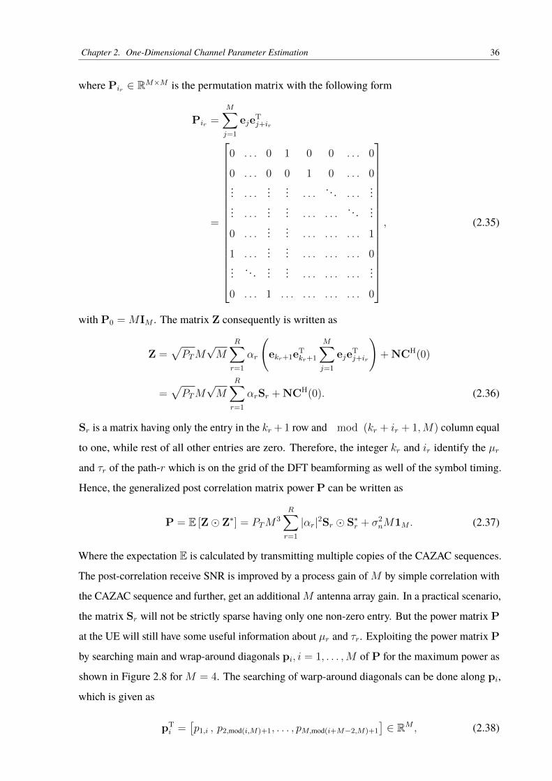
by searching main and wrap-around diagonals pi, i = 1, . . . ,M of P for the maximum power as

shown in Figure 2.8 for M = 4. The searching of warp-around diagonals can be done along pi,

which is given as

pTi =

[p1,i , p2,mod(i,M)+1, . . . , pM,mod(i+M−2,M)+1

]∈ RM , (2.38)


p11

p1 p3

p12 p13 p14

p21 p22 p23 p24

p31 p32 p33 p34

p41 p42 p43 p44

Figure 2.8 – An example of integer delay estimation τi using power matrix P as in (2.37) wherep1 and p3 are the two diagonals, for which (2.39) is fulfilled.

where i = 1, . . . ,M . For i = 1 we have p1, which is the main diagonal of power matrix P. We

search all the diagonals i = 1, . . . ,M , whether the maximum power exceeds the threshold G as

maxk=1,...,M

(pk,mod(i+(k−2),M)+1

)≥ G, i = 1, . . . ,M. (2.39)

G should be heuristically chosen to make sure that the received signal is above the noise floor

which in our case is σ2nM . The coarse estimates for the integer delay τir for path-r is shown in

Figure 2.8

τir = ir − 1. (2.40)

For the main diagonal p1, we always assume LOS path, where the delay τi = i1−1∣∣i1=1

= 0. The

number of diagonals fulfilling (2.39) results in the coarse estimation of the model order R with

the corresponding coarse estimates of τir , where we drop the index r for notational convenience.

As we know, the actual spatial frequency for each path-r lies somewhat in between

two spatial frequencies Φk < µr < Φk+1, which ends up with two significant received powers

denoted by Pk and Pk+1 as shown in Figure 2.9.

LUT: To have a coarse estimate of µr, we construct a LUT which is necessary for

the linear interpolation having D + 1 spatial frequencies µd, generated as

µd = Φk + d∆µ, d = 0 . . . , D (2.41)

∆µ =Φk+1 − Φk

D=

2π

MD. (2.42)

Now we compute the hypothetical noise free normalized power based on these µd, which is given

as

Pk,d =∣∣aH(µd)w(Φk)

∣∣2 (2.43)

Pk+1,d = |aH(µd)w(Φk+1)|2. (2.44)


Figure 2.9 – An example of coarse estimation using DFT matrix based beamforming.

where a(µd) is the channel steering vector and defined as,

a(µd) =[1, e−jµd , . . . , e−j(M−1)µd

]T ∈ CM×1. (2.45)

Calculating the ratio of the hypothetical powers as

∆d =

√Pk,dPk+1,d

. (2.46)

Since hypothetical powers Pk,d and Pk+1,d are independent of k, means the difference between

any two consecutive beams is the same, therefore we just needD+1 ratios to fill into the so-called

LUT, respectively. Note that, the LUT once generated is fixed for any coarse estimation of the

spatial frequency µr.

Coarse estimation of µr: Now to estimate µr based on the setup LUT, we choose

those indices d and d+1 in the LUT, where the two corresponding ratios ∆d and ∆d+1 are closest

to the ratio, which the UE has calculated in (2.47)

∆ =

√PkPk+1

(2.47)

The coarse estimate of µr is calculated using linear interpolation as

µr = µd + b∆µ = Φk + ∆µ(d+ b). (2.48)

where the constant b is given as

b =∆d −∆

∆d −∆d+1

. (2.49)


Algorithm 2.1: Propose coarse estimation algorithm for estimation of θr.1 Require: Y (2.31) ;2 The UE received Y and get pi for each path r (2.37);3 Calculate ∆ as in (2.47);4 Find d such that ∆d ≥ ∆ ≥ ∆d+1;5 Calculate constant b as in (2.49);6 Return µr and θr as in (2.48) and (2.50).;

Finally, the conversion from spatial frequency µr to azimuth AoD θr

θr =

arcsin( µrπ

), 0 ≤ µr ≤ π,

arcsin( µr−2ππ

), π < µr ≤ 2π.

(2.50)

The interpolation between Φk and Φk+1 might go wrong in cases where the received signal level

is weak and let say µr is very close to the beamforming angle Φk. In this case, Pk might be

quite large, but Pk+1 might be close to the noise floor. Therefore, for the receiver, it is difficult to

decide whether Pk+1 or Pk−1 is the second largest power to be used in interpolation due to being

masked by noise. Hence, we check whether

|Pk+1 − Pk−1| ≤σ2n

v. (2.51)

If (2.51) is satisfied, then it is not worthwhile to interpolate but simply choose µr = Φk. We

heuristically chosen v = 3 in our numerical experiments. The complete method is shown in

Algorithm 2.1

After estimated all AoDs, the model order estimation may be refined, because of the

integer estimation of the delays. One non-integer delay may have lead to two adjacent integer

delays, and both of them will have the same AoD estimate. If this occurs, we drop one of the

two delays. Furthermore, we can also use a model order detection algorithm given in [48] before

feeding the coarse parameters to the SAGE algorithm for the refinement of parameters.

There is still the question, how well this coarse estimation is capable of resolving

two paths, which are close to each other in the spatial frequency domain and in the delay domain.

If there is a delay difference between the two paths of approximately one symbol period or more,

then the spatial frequencies can be arbitrarily close and the paths can still be separated. On the

other hand, if the difference of the spatial frequencies is at least 2πM

(the difference between two

adjacent beam patterns), then the two paths could be resolved even if the delay difference is

arbitrarily small. Therefore, the proposed coarse estimation scheme is of high resolution in either

of the spatial frequency domain or in the delay domain, but not in both simultaneously.


2.4.3 ML Estimation Using SAGE

Let us assume a random matrix Y which has a multivariate complex Gaussian pdf

which is parametrized by the unknown channel parameter vector η as

η =[√

PTRe{α}T,√PT Im{α}T,µT, τT

]T

. (2.52)

where

√PTRe{α} =

[√PTRe{α1}, . . . ,

√PTRe{αr}, . . . ,

√PTRe{αR}

]T

, (2.53)

√PT Im{α} =

[√PT Im{α1}, . . . ,

√PT Im{αr}, . . . ,

√PT Im{αR}

]T

, (2.54)

µ = [µ1, . . . , µr, . . . , µR]T , (2.55)

τ = [τ1, . . . , τr, . . . , τR]T . (2.56)

The likelihood function is

L(Y;η) =1

πML det Rexp

−vec

{Y −

√PT

R∑r=1

αrA(µr)C(τr)

}H

R−1 vec

{Y −

√PT

R∑r=1

αrA(µr)C(τr)

}). (2.57)

The ML estimator is given as

η = arg maxη

L (Y;η) , (2.58)

whereas no closed form solution can found for the ML estimator because (2.58) is a multidimen-

sional, non-linear optimization problem. We use the SAGE algorithm [49] to solve our non-linear

problem. We configure the SAGE algorithm for our scenario and ends up with the following

expectation-maximization steps,

Expectation step:

Xr = Y −R∑

r′=1r′ 6=r

Sr′(ηr′). (2.59)


where

Sr(ηr) =√PTαrA(µr)C(τr). (2.60)

Maximization step:

τr = arg maxτr

∣∣∣tr{CH(τr)A

H(µr)Xr

}∣∣∣2βrσ2

n tr{CH(τr)AH(µr)A(µr)C(τr)}

, (2.61)

µr = arg maxµr


H(µr)Xr

}∣∣∣2βrσ2


. (2.62)

Finally, ˆ√PTα can be found as

ˆ√PTαr =

tr{

CH(τr)AH(µr)Xr

}tr{CH(τr)AH(µr)A(µr)C(τr)}

. (2.63)

The derivation is given in Appendix A.3.

2.4.3.1 Convergence analysis of SAGE

The second stage of the two-stage algorithm is to refine the coarse estimate using the

ML estimator. To make sure that the SAGE algorithm converges to the global optimum using

very few iterations is of practical interest. To achieve this, it is mandatory to start the SAGE

algorithm with a good coarse estimate of the parameters achieved using PREIDG algorithm. We

use τi (2.40), µr (2.48) and αr = 0 to initialize the SAGE in the second stage of the algorithm.

One iteration of the SAGE algorithm is as a full update of the parameter vector η. The stopping

thresholds for the SAGE convergence are given as

T1 =|µrp − µr||µr|

, (2.64)

T2 =|τrp − τr||τr|

, (2.65)

T3 =| ˆ√PTαrp −

ˆ√PTαr|

| ˆ√PTαr|, (2.66)

where µrp , τrp , ˆ√PTαrp , are the previous estimates of spatial frequency, delay time and complex

path gain. The SAGE algorithm approach approximately the global optimum when (2.67) is


Figure 2.10 – A flowchart for the two-stage estimation algorithm.

fulfilled as

max {T1,T2,T3} ≤ Γ, (2.67)

Γ represents the stopping threshold.

The two-stage algorithm is shown in Figure 2.10.

2.4.4 CRLB

In this section, we derived the FIM F(η) for providing a theoretical lower bound on

the estimation errors of the channel parameters η to assess the performance our approximated

ML estimates.

Assuming η as an unbiased estimator of η, then the variance var of the estimation error can be


lower-bounded by the diagonal elements of the inverse of F(η) [46]


]i i. (2.68)

The FIM for the complex data can be given as

[F(η)]ij =2

σ2n

Re

{tr

{∂SH(η)

∂ηi

∂S(η)

∂ηj

}}, (2.69)

where the matrix S(η) is

S(η) =R∑r=1

S(ηr) =√PT

R∑r=1

αr A(µr) C(τr) (2.70)

where

ηr =[√

PTRe{αr},√PT Im{αr}, µr, τr

]. (2.71)

The FIM F(η) can be structured as

F(η) =

FRe{α}Re{α} FRe{α}Im{α} FRe{α}µ FRe{α}τ

FTRe{α}Im{α} FIm{α}Im{α} FIm{α}µ FIm{α}τ

FTRe{α}µ FT

Im{α}µ Fµµ Fµτ

FTRe{α}τ FT

Im{α}τ FTµτ Fττ

. (2.72)

The entries of the F(η) (2.72) are derived in Appendix A.4.


In this section, the performance of the proposed two-stage algorithm is analyzed and

assessed with CRLB and compared with the ABP method [26] by computer simulations. The

transmitter at the BS station uses the PCBM hybrid architecture with the BM used for exciting

the ULA with M = 16 antennas, using the inter-element spacing d = λ/2. Furthermore, we

assume only one subarray for channel probing in a round-robin fashion. We assume the carrier

frequency of the system fc = 28 GHz and bandwidth of the system as B = 200 MHz giving a

symbol duration Ts = 5 ns. We use 32 pilot symbols per beam for channel probing which leads

to the total number of 512 QPSK symbols as pilot overhead. We model our channel parameters

based on [47]. The distance for the LOS among the BS and UE is uniformly distributed as

Xlos ∼ U(30 m, 60 m). (2.73)

Similarly, the NLOS distance are uniformly distributed as


Table 2.1 – Beamforming angles using one 16× 16 BMS.No beamforming vector spatial frequency Φk AoD θ◦k

1 w(Φ0) 0 02 w(Φ1) π/8 7.18083 w(Φ2) π/4 14.47754 w(Φ3) 3π/8 22.02435 w(Φ4) π/2 306 w(Φ5) 5π/8 38.68227 w(Φ6) 3π/4 48.59048 w(Φ7) 7π/8 61.04509 w(Φ8) π 9010 w(Φ9) 9π/8 −61.045011 w(Φ10) 5π/4 −48.590412 w(Φ11) 11π/8 −38.682213 w(Φ12) 3π/2 −3014 w(Φ13) 13π/8 −22.024315 w(Φ14) 7π/4 −14.477516 w(Φ15) 15π/8 −7.1808

Xnlos = Xlos + ∆nlos, (2.74)

where ∆nlos is the difference between LOS and NLOS component and is distributed as ∆nlos ∼

U(4.5 m, 24 m) which ends up with a delay difference between 3 and 16 symbols. The length of

CAZAC sequence L = 16 restricts the maximum delay difference to be estimated. The path loss

can be given as

PL(dB) = 10n log10

(X

X0

), (2.75)

where n represents the path loss exponent which is chosen as 2.1 and 2.4 for LOS and NLOS

respectively. X0 is assumed as one meter. γr is magnitude of the complex path gain of each path-r

and is defined as the ratio of the path loss for LOS (PLlos) and NLOS (PLnlos) respectively.

γr =

√PLlos

PLnlos. (2.76)

The complex path gain αr for each path-r can be given as

αrα1

= γrejϕr , (2.77)

where α1 is the complex path gain of the LOS and assumed as one. ϕr is the phase of the complex

path coefficient. For every path-r, it is generated as ϕr ∼ U(0, 2π). Note that the phase of the

complex gain ϕr is different for every sub-array at BS while the magnitude γr is the same for

every sub-array. In this approach, as the BS knows the geometry of the antennas array, it can

estimate the phase of the other sub-arrays based on the estimation of the phase ϕ1 of the first array.


The AoD’s θr for LOS and NLOS can be generated simultaneously as being uniformly distributed

over one sector of a cell θ◦r ∼ U(−60◦,+60◦). The noise variance is assumed as σ2n = 1. The

total number of paths is assumed as R = 3. The spatial frequencies and their respective AoD

azimuth angles in degrees are given in Table 2.1. The SNR is defined as

SNR =PT |α1|2

σ2n

. (2.78)

The RMSE for the channel parameter can be given as

Figure 2.11 – Histogram for the number of iterations of SAGE in the two-stage algorithm.

RMSE(θr) =

√E[|θr − θr|2

](2.79)

RMSE(ˆ√PTαr) =

√√√√√E

∣∣∣∣∣√PTαr − ˆ√PTαr√

PTαr

∣∣∣∣∣2 (2.80)

RMSE(τr) =√E [|τr − τr|2]. (2.81)

The bound on the error is calculated as

√CRLB(ηi) =

√[F−1(η)]i i. (2.82)

We use 10000 channel realizations for calculating the RMSE for each parameter at different

SNRs and similarly, the CRLB for each parameter is obtained by numerical averaging over 10000

channel scenarios. The length of the look-up/interpolation table for the PREIDG algorithm is

assumed as D = 101.


-5 0 5 10 15 20

SNR(dB)

10-2

10-1

100

101

Figure 2.12 – Performance comparison of two-stage and ABP algorithm for LOS AoD,assuming R = 3.

To form beam pairs in the ABP method using a DFT matrix, we fixed δ = 2mπM

= π8,

assuming m = 1 [26]. The 16 beam pairs can be represented as (1, 3), (2, 4), . . . , (15, 1), (16, 2).

The criteria for choosing the auxiliary beam pair out of all the 16 beam pairs is the one that gives

the maximum average power.

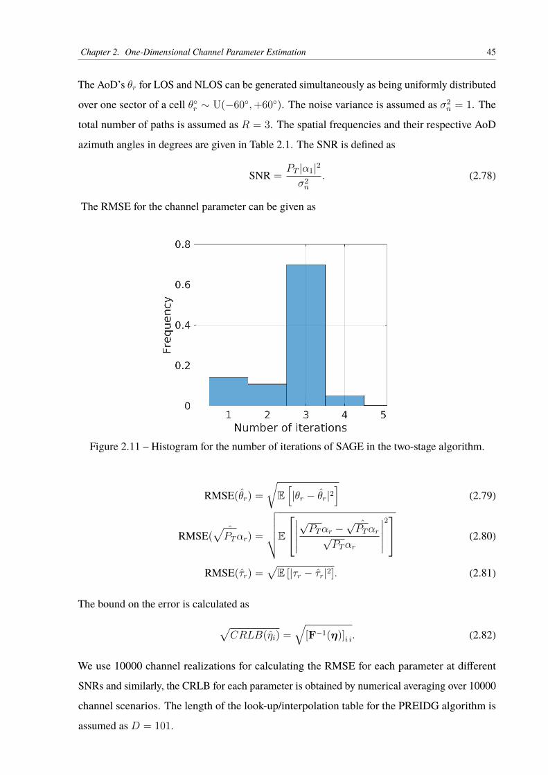
The motivation behind the two-stage algorithm is to reduce the number of iterations

for the convergence of the SAGE and assure it to achieve the global optimum. For this reason,

an additional coarse estimation based on PREIDG is performed before the SAGE algorithm is

initialized. Now with initialization of the SAGE algorithm with µr (2.48), integer delay τi (2.40),√PTαr = 0, and fixing the threshold Γ = 10−3, which facilitate the convergence of the SAGE

algorithm with maximum number of 4 iterations. In 70% of the channel realizations, SAGE

took 3 iterations to converge, which is shown in Figure 2.11. In the low SNR regime, during the

coarse estimation, we are also doing the model order estimation due to which the NLOS paths

are not always detected and, unable to estimate in every channel realization because of the high

path-loss. While in the high SNR regime, we can detect almost all paths.

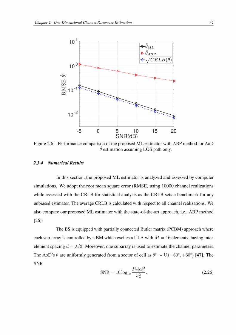
Figure 2.12 shows the performance of the proposed two-stage algorithm as compared

with the ABP method. Simulation results based on 10 thousands of channel realizations show

that the proposed PREIDG method performs better than ABP. Furthermore, it shows that the

resolution of the PREIDG algorithm improves by increasing SNR. After using coarse estimation

based on PREIDG, as an ad-hoc estimation to initialize the SAGE algorithm gives the improved

ML performance which nearly satisfies the theoretical bound.


Similarly, the AoDs performance of the two-stage method for NLOS paths are compared with

-5 0 5 10 15 20

SNR(dB)

10-2

10-1

100

Figure 2.13 – Performance comparison of two-stage and ABP algorithm for NLOS AoD,assuming R = 3.

ABP and is assessed with theoretical CRLB in Figure 2.13. The performance of PREIDG still

performs better than ABP for NLOS paths. The performance of the ML approach performs better

than both PREIDG and ABP method. The ML method approaches the CRLB closely.

-5 0 5 10 15 20

SNR(dB)

10-3

10-2

10-1

100

Figure 2.14 – Performance comparison of two-stage and ABP algorithm for αr.

Figure 2.14 shows the comparison of the two-stage algorithm with the ABP method.

The proposed two-stage algorithm shows a better performance for the estimation of the complex

path gain ˆ(√PTαr) as compared to the ABP method. In addition, the ML estimate as a result


of the two-stage algorithm for ˆ(√PTαr) approximately approaches the theoretical CRLB. We

assume α1 = 1 for LOS path.

-5 0 5 10 15 20

SNR(dB)

10-2

10-1

Figure 2.15 – Performance comparison of two-stage algorithm for τr

The two-stage estimation algorithm is evaluated for delay time τr in fractions of

symbol period as shown in Figure 2.15. The result is the output of the two-stage algorithm which

approximates ML estimate for τr which nearly approaches the theoretical CRLB. The delay time

for LOS is assumed as τ1 = 0. The combining of coarse estimation based on a PREIDG algorithm

to initialize the SAGE algorithm enhances the estimation accuracy. The ABP algorithm is unable

to estimate the delay time τr.

Keep in mind that we can also use ABP method for coarse estimation but it is not

guaranteed that the SAGE algorithm will converge to the global optimum. This is because that

the ABP method is unable to estimate the time-delay for each path.

49

3 TWO-DIMENSIONAL CHANNEL PARAMETER ESTIMATION

This chapter introduces the two-dimensional channel parameter estimation (azimuth

and elevation angle of departure, complex-path gain and time delay) using a two-stage algorithm.

In the first stage, a coarse estimation is based on modified PREIDG using Kronecker products of

DFT beams while high-resolution parameter estimation is done using the SAGE algorithm. To

assess the performance of the SAGE algorithm, CRLB is derived in addition to the comparison

of a modified PREIDG algorithm with the ABP method.

3.1 Overview

To realize two-dimensional beamforming for the next-generation mobile commu-

nication systems, an URA is introduced which simplifies multiuser spatial separation in a cell

while maximizing the available data rates and minimizing the inter-user interference. Employing

large antenna arrays at the BS is a challenge that is tackled by introducing hybrid beamform-

ing with a PCAPS network using Butler matrices (BMs) termed as partially connected Butler

matrices (PCBMS) approach in the analog domain to ensure energy efficient implementation

[50, 51, 45, 52]. The idea is to extend the ULA excited by a single BM as discussed in [50, 51] to

a two-dimensional URA, which is of more practical interest. We propose a new way of combing

BMs to excite an URA as shown in Figure 3.1. In this two-dimensional network of BMs, the

resultant beamforming vector is the Kronecker product of the columns of DFT

w(δp, νq) = wh(δp)⊗wv(νq) ∈ CM×1, (3.1)

where w (δp, νq) is the resultant beamforming vector for probing the channel. δp is the DFT

spatial frequency of the DFT matrix controlling the horizontal antenna elements, and wh(δp) is

defined as

wh(δp) =1√Mh

[1, e−jδp , . . . , e−j(Mh−1)δp

]T ∈ CMh×1, (3.2)

where δp = 2πMhp, p = 0, . . . ,Mh − 1. Mh is the number of antenna elements on the horizontal

axis. νq is the DFT spatial frequency of the DFT matrix exciting the vertical antenna elements in

the URA, and wv(νq) is defined as

wv(νq) =1√Mv

[1, e−jνq , . . . , e−j(Mv−1)νq

]T ∈ CMv×1, (3.3)

νq = 2πMvq, q = 0, . . . ,Mv − 1. Mv represents the number of antenna elements on vertical axis.

Chapter 3. Two-Dimensional Channel Parameter Estimation 50

Figure 3.1 – An architecture of BMs exciting two-dimensional uniform rectangular array.

Figure 3.2 – A 4-point DFT building block.

3.1.1 Construction of 4× 4 BM

The fast Fourier transform (FFT)-signal-flow graph (SFG) for a 4× 4 DFT matrix

multiplication is accomplished with eight complex additions and one complex multiplication as

shown in Figure 3.2, with the following expressions,b1

b2

b3

b4

=1

2

1 1 1 1

1 −j −1 j

1 −1 1 −1

1 j −1 −j

a1

a2

a3

a4

. (3.4)

There is a total of four butterflies in the construction of 4-point DFT matrix. To design 4× 4

microwave circuit, i.e., BM using 90◦ hybrid coupler as shown in Figure 2.4, we need to replace

the one butterfly with one 90◦ hybrid coupler as given in (2.2) with two PSs and one additional

−90◦ fixed PS as shown in Figure 3.3.


90o hybrid

Figure 3.3 – A 4× 4 BM using 90◦ hybrid couplers.

3.2 Contributions

The contribution and the organization of the chapter is as

• System Model: In this section, the system model is based on a two-dimensional URA

excited by the network BMs in the analog domain.

• Coarse estimation based on modified PREIDG:

In this section, the coarse estimation is performed based on the modified PREIDG.

• SAGE:

We derive and configure SAGE algorithm for the non-linear problem to achieve high-

resolution parameter estimation by initializing with coarse estimates achieved using modi-

fied PREIDG.

• CRLB:

We derive the CRLB for high-resolution channel parameter estimation considering MISO

system where the BS is equipped with an URA and the UEs have a single antenna each.

• Simulation results: In this section, we show extensive simulations to evaluate the per-

formance of the proposed modified PREIDG and compare it with the ABP method [27].

We further show that, initializing the SAGE algorithm with the coarse estimates achieved

using modified PREIDG algorithm can nearly approache the CRLB.


1. Design of the two-dimensional beamformer with hardware constraints. We introduce

new way of combining BMs to excite the URA. The new architecture is energy-


efficient and has less implementation complexity in the analog domain.

2. A novel two-stage algorithm for the two-dimensional parameter estimation is proposed,

where an efficient way of coarse estimation is achieved based on modified PREIDG

algorithm followed by the refinement stage done by the SAGE algorithm.

3. Derivation of the CRLB for the assessment of the SAGE algorithm. The modified

PREIDG is compared with the ABP method [27].

3.3 Two-Dimensional Parameter Estimation Algorithm for Frequency Selective Channel

In the section, a novel two-dimensional two-stage algorithm is proposed and discussed.

A coarse estimation based on the modified PREIDG is used to the SAGE algorithm to achieve

high-resolution parameter estimation.

3.3.1 System Model

We consider a single-cell downlink scenario for a frequency selective channel con-

sidering a MISO system where the BS is equipped with N antennas. The BS employs a PCBMS

approach [50, 51] where each sub-array is composed of M antennas satisfying N = NRF ×M ,

controlled by NRF chains. The two-dimensional mth beamforming vector wm (δp, νq) is used to

probe the channel with a specific CAZAC [53, 54, 55] sequence, leading to the resulting received

vector ym ∈ CL×1 per one sub-array

yTm =

√PT

R∑r=1

αraH(φr, θr)wm(δp, νq)c

Tm(τr) + nT

m, (3.5)

where m = q + pMv, p ∈ {0, . . . ,Mh − 1}, q ∈ {0, . . . ,Mv − 1}, and m ∈ {0, . . . ,M − 1}

given that M = MhMv. PT is the transmit power, αr is the complex gain of each path r, cm

is the specific CAZAC sequence with length L having one-to-one correspondence with the

two-dimensional beamforming vector wm (δp, νq), nm ∼ CN (0L×1, σ2nIL) is the noise vector,

where σ2n is the noise variance, φr is the azimuth AoD, θr is the elevation AoD, a(φr, θr) is

the two-dimensional steering vector of a URA in the y-z-plane with inter-elements distance as

dh = dv = λ/2 as,

am(φr, θr) = e−jπ[p sin θr sinφr+q cos θr] (3.6)

The URA has Mh antenna elements in the y direction and Mv elements in the z direction

with M = MhMv as shown in Figure 3.4. Now, let us consider the two-dimensional steering


vector a (φr, θr) given in (3.6) and define the spatial frequencies as µr = π sin θr sinφr and

ψr = π cos θr respectively. Therefore, the steering vector can be re-written as

a(µr, ψr) = [a0(µr, ψr), a1(µr, ψr), . . . , aM−1(µr, ψr)]T . (3.7)

Furthermore, (3.7) can also be re-written as the Kronecker product using the following steering

vectors

ah(µr) =[1, e−jµr , . . . , e−j(Mv−1)µr

]∈ CMv×1, (3.8)

and

av(ψr) =[1, e−jψr , . . . , e−j(Mh−1)ψr

]∈ CMh×1. (3.9)

Hence, the channel steering vector a (µr, ψr) can also be written as

a(µr, ψr) = ah(µr)⊗ av(ψr) ∈ CM×1. (3.10)

The CAZAC sequence specific for each beamforming vector is cm, where each symbol c0 is

constructed as

c(n) = e

(j 2π√

L(mod{n,√L}+1)

(⌊n√L

⌋+1)

+j π4

), (3.11)

where n ∈ {0, 1, . . . , L− 1} and cm is an m-fold wrap-around version of c0. By probing all the

two-dimensional beamforming vectors with their specific CAZAC sequences and collecting all

the receive vectors ym in the matrix Y ∈ CM×L as

Y =√PT

R∑r=1

αrA(µr, ψr, δp, νq)

cT

0 (τr)

cT1 (τr)

...

cTM−1(τr)

︸︷︷︸

=C(τr)

+

nT

0

nT1

...

nTM−1

︸︷︷︸

=N

, (3.12)

and rewriting

Y =√PT

R∑r=1

αrA(µr, ψr, δp, νq)C(τr) + N, (3.13)

where A(µr, ψr, δp, νq) ∈ CM×M is represented as

A(µr, ψr, δp, νq) = diag{aH(µr, ψr)w(δp, νq)

}M−1

m=0, (3.14)


unit ball

wavefront

Figure 3.4 – Uniform planar array in y-z-plane.

and the noise covariance matrix is


]= σ2

nIML, (3.15)

assuming spatially and temporally uncorrelated noise.

3.3.2 Coarse estimation based on modified PREIDG

In the two-stage estimation algorithm, the first stage is responsible for estimating the

model order and the channel parameters which are achieved by the modified PREIDG. We useM

CAZAC sequences of length L = M having one-to-one correspondence to M two-dimensional

beamforming vectors which are used to probe the channel. This way each UE observes M

consecutive sequences ym (3.5) and the received signals are multiplied with stored CAZAC

sequences c∗m and can be formulated for one UE as

Z = YCH(0) =√PT

R∑r=1

αrA(µr, ψr, δp, νq)C(τr)CH(0) + NCH(0), (3.16)

where C(0) ∈ CM×L is the CAZAC sequences matrix with time-delay equal to zero. Further,

the post-correlation power matrix P can be given as

P = E [Z� Z∗] . (3.17)

Now, in any real scenario, the matrix P will not be sparse but can provide useful information

about the model order, i.e., the number of multipath, and the channel parameters such as√PT , αr,


ψr, µr and τr of each path. We exploit the power matrix by searching the (wrap-around) diagonals

pTir =

[p1,i , p2,mod(i,M)+1, . . . , pM,mod(i+M−2,M)+1

]∈ RM , (3.18)

where i = 1, . . . ,M , with p1 being the main diagonal of matrix P (3.17). For each diagonal pi

we check, whether the largest element is above a certain threshold G as,

maxk=1,...,M

(pk,mod(i+(k−2),M)+1

)≥ G, i = 1, . . . ,M. (3.19)

G should be chosen such that we can detect signals above the noise floor σ2nM . The integer delay

τir for each rth path can be found as

τir = ir − 1. (3.20)

For the main diagonal p1, this will always be fulfilled assuming a LOS path, which has delay

τi = i1 − 1∣∣i1=1

= 0. The number of diagonals pi, which fulfill (3.19) is the estimated model

order R and provide a coarse estimate τir for each path, i.e., the estimated integer delay where

the index r is dropped for notational convenience in the subsequent sections.

3.3.3 LUT

To get coarse estimates of the spatial frequencies µr and ψr, we design only one LUT,

which will be used for both, the azimuth beamforming angles δp and the elevation beamforming

angles νq. We show this in detail for µr, where we use linear interpolation with D + 1 spatial

frequencies µd given as

µd = δp + d∆µ, d = 0, . . . , D, (3.21)

with

∆µ =δp+1 − δp

D=

2π

MhD. (3.22)

Now, computing the hypothetical noise free normalized power using the hypothetical spatial

frequencies µd can be given as

Pp,d =∣∣aH(µd)wh(δp)

∣∣2 , (3.23)

and

Pp+1,d = |aH(µd)wh(δp+1)|2, (3.24)


p11 p12 p13 p14

p21 p22 p23(max) p24

p31 p32 p33 p34

p41 p42 p43 p44

Figure 3.5 – Two-dimensional power-table P′r for estimation of spatial frequencies µr and ψr.

where the channel steering vector for hypothetical spatial frequency a(µd) can be written as

a(µd) =[1, e−jµd , . . . , e−j(Mh−1)µd

]T ∈ CMh×1. (3.25)

The ratio of the hypothetical powers can be given as

∆d =

√Pp,dPp+1,d

. (3.26)

Since the hypothetical powers Pp,d and Pp+1,d are independent of p, meaning, the difference

between two consecutive beams is same, therefore we just need D + 1 ratios to fill into the

so-called LUT, respectively. Note that, the only one LUT, once generated is fixed and the same

LUT can be used for ψr.

3.3.4 Estimation of Spatial Frequencies

In this section, after estimating the model order R, the spatial frequencies are esti-

mated in the following way. Let us assume pr ∈ CM×1 being the diagonal or cross diagonal vector

of the received power matrix P ∈ CM×L for the rth path as given in (3.18), where MhMv = M .

Now, by un-vectorizing the selected pr as

P′r = unvec{pir}T ∈ CMh×Mv . (3.27)

Now we have to assign to every entry of P′r the beamforming vector, with which the corresponding

post correlation power value has been generated.

We see that [P′r]maxp+1,q+1 as shown in Figure 3.5, i.e., the entry in the p + 1th row and q + 1th


Algorithm 3.1: Two-dimensional parameter estimation of µr based on modifiedPREIDG.1 Require: Y (3.12) ;2 Determine pir from (3.17) and (3.18);3 Re-arrange pir in the power matrix P′r as shown in (3.27);4 Find the highest power [P′r]

maxp+1,q+1 and the associated beamforming vector w (δp, νq) ;

5 Find the second power in the q + 1th column [P′r]p+2,q+1 and the associatedbeamforming vector w (δp+1, νq) ;

6 Calculate ∆µr as in (3.29);7 Find d such that ∆d ≥ ∆µr ≥ ∆d+1 as in (3.26) ;8 Calculate constant bµ as in (3.31);9 Return µr as in (3.30). ;

column of P′r has been generated by the following beamforming vector,

w (δp, νq) = wh(δp)⊗wv(νq). (3.28)

Let us assume that the second largest entry in the p+1th row is [P′r]p+1,q and in the q+1th column

is [P′r]p+2,q+1. Then the interpolation for µr should be carried out between δp < µr < δp+1 and

for ψr between νq−1 < ψr < νq.

Now let us use the LUT which we produced according to (3.21)-(3.26) and let us choose those

indices d and d+ 1 such that ∆d and ∆d+1 are the two ratios closest to

∆µr =

√[P′r]p+1,q+1

[P′r]p+2,q+1

. (3.29)

We estimate µr as

µr = µd + bµ∆µ, (3.30)

with

bµ =∆d −∆µr

∆d −∆d+1

. (3.31)

The µr estimation approach is given in Algorithm 3.1. The same procedure can be adapted for

estimating ψr.

3.3.5 Example with a 4× 4 URA

Let us take 4×4 URA havingMh = 4 andMv = 4 with the total number of antennas

at each subarrayM = 16. Therefore, by defining the horizontal and vertical beamforming vectors

as

wh(δp) =1

2

[1, e−jδp , e−j2δp , e−j3δp

]T, (3.32)


1 2 3 4 5 6 7 8 9 10 11 12 13 14 15 16w(δ0, ν0) p11

w(δ0, ν1) p12

w(δ0, ν2) p13

w(δ0, ν3) p14

w(δ1, ν0) p21

w(δ1, ν1) p22

w(δ1, ν2) p23

w(δ1, ν3) p24

w(δ2, ν0) p31

w(δ2, ν1) p32

w(δ2, ν2) p33

w(δ2, ν3) p34

w(δ3, ν0) p41

w(δ3, ν1) p42

w(δ3, ν2) p43

w(δ3, ν3) p44

Figure 3.6 – An example for constructing received power matrix P considering a 4× 4 URA.

and

wv(νq) =1

2

[1, e−jνq , e−j2νq , e−j3νq

]T, (3.33)

where δ0 = ν0 = 0, δ1 = ν1 = π2, δ2 = ν2 = π, δ3 = ν3 = 3π

2. The resultant two-dimensional

beamforming vector can be written as

w(δp, νq) = w(δp)⊗w(νq) =

1

4

[1, e−jνq , e−j2νq , e−j3νq , e−jδp , e−j(δp+νq), e−j(δp+2νq)

e−j(δp+3νq), . . . , e−j(3δp+2νq), e−j(3δp+3νq)]T. (3.34)

When generating the power matrix P (3.17), each row is obtained with one beamforming vector

w(δp, νq), i.e., with one index pair (p, q) as shown in Figure 3.6.

Let us assume that the rth path has a integer-delay τir = 6. The diagonal pir looks as follows:

pir = [p11, . . . , p14, p21, . . . , p24, p31, . . . , p34, p41, . . . , p44]T , (3.35)

and

P′r = unvec{pir}T =

p11 p12 p13 p14

p21 p22 p23 p24

p31 p32 p33 p34

p41 p42 p43 p44

. (3.36)


Therefore, the power entry [P′r]p+1,q+1 has been produced with w(δp, νq).

Now let us take an example for a demonstration with a UE position at AoD azimuth φ = 35◦ and

elevation θ = 95◦ as shown in Figure 3.7. The largest element of P′r is p21, the two next largest

ones are p31 and p24. The three corresponding beamforming vectors should be

Beam 1 : w(δ1, ν0) with φ1,0 = 30◦, θ1,0 = 90◦

Beam 2 : w(δ2, ν0) with φ2,0 = 90◦, θ2,0 = 90◦

Beam 3 : w(δ1, ν3) with φ1,3 = 35.2644◦, θ1,3 = 120◦.

The corresponding positions in the P′r matrix should be for

Beam 1 : [P′r]2,1 = [P′r]max2,1

Beam 2 : [P′r]3,1

Beam 3 : [P′r]2,4 .

Therefore, the interpolation for µr should take place between δ1 and δ2 which correspond to beam

1 and beam 2 respectively. Similarly, the interpolation for ψr should take place between ν3 and

ν0, which correspond beam 3 and beam 1 respectively.

Since δp and νq in the DFT matrices are in the range [0, 2π), and Algorithm 3.1

considers them in the range (−π, π], the following transformation is applied:

x = mod(x+ π, 2π)− π, x ∈ {δp, νq, µr, ψr}. (3.37)

Finally, to get an estimate for the azimuth φr and the elevation θr as,

θr = arccos

(ψrπ

), (3.38)

φr = arcsin

(µr

π sin(θr)

), (3.39)

with the range of θ◦r ∼ U(90◦, 130◦) and φ◦r ∼ U(−60◦, 60◦).

Note: The interpolation between δp and δp+1 for estimating µr, and similarly the interpolation

between νq−1 and νq for estimating ψr can go wrong in some cases, especially if the signal level

is weak. Consequently, let us say that µr is close to the δp with highest received power, but the

received power generated using δp+1 may be close to the noise floor and similarly let us say that


(a) Maximum power received using beam-1w (φ1,0 = 30◦, θ1,0 = 90◦)

(b) Second-highest power received usingbeam-2 w (φ2,0 = 90◦, θ2,0 = 90◦)

(c) Second-highest power received usingbeam-3 w (φ1,3 = 35.2644◦, θ1,3 = 120◦)

Figure 3.7 – An example of two-dimensional coarse estimation via three two-dimensionalbeamforming vectors for the UE at (φ = 35◦, θ = 95◦)

ψr is close to νq with highest received power but the received power generated using νq−1 may

be close to the noise floor. Therefore, we check whether|[P′r]p+1,q+2 − [P′r]p+1,q| ≤ σ2

n,

|[P′r]p+2,q+1 − [P′r]p,q+1| ≤ σ2n.

(3.40)

If (3.40) is fulfilled, then it is not worthwhile to interpolate at all, but simply choose µr = δp,

and ψr = νq.

3.3.6 High-resolution channel parameter estimation using SAGE

High-resolution parameter estimation in general is of practical interest for wireless

communication systems. High-resolution channel parameter estimation plays an important role

in designing hybrid precoders at the BS because the channel parameters need to be quantized

before being sent back to the BS. The BS receives the channel parameters with quantization error

resulting in deterioration of the performance. The deterioration can be increased if the channel


parameters are not estimated with high accuracy.

It is also known in the literature that SAGE and ESPRIT are high-resolution estimation algorithms

[36], but the SAGE algorithm can provide the highest accuracy as compared to MUSIC and

ESPRIT [37, 56, 57, 58]. On the the other hand, ESPRIT has less computational complexity as

compared to the standard SAGE algorithm, however, ESPRIT needs two translation invariant

subarrays in the URA while on the other hand SAGE does not impose such kind of an assumption.

To ensure a high-resolution parameter estimation with less computational complexity, we initialize

the SAGE algorithm with coarse estimates achieved by the modified PREIDG algorithm. We use

the fundamental principles of the SAGE algorithm [59, 49] to derive new expressions for our

non-linear problem at hand. Furthermore, using SAGE, a refined estimate of complex path gain

and non-integer delay can be achieved.

Let us assume a random variable Y as given in (3.12) having a multivariate complex Gaussian

pdf which is parametrized by the unknown channel parameter vector η as

η =[√

PTRe{α}T,√PT Im{α}T,µT,ψT, τT

]T

, (3.41)

where √PTRe{α} =

[√PTRe{α1}, . . . ,

√PTRe{αR}

]T

∈ CR×1, (3.42)√PT Im{α} =

[√PT Im{α1}, . . . ,

√PT Im{αR}

]T

∈ CR×1, (3.43)

µ = [µ1, . . . , µR]T ∈ CR×1, (3.44)

ψ = [ψ1, . . . , ψR]T ∈ CR×1, (3.45)

τ = [τ1, . . . , τR]T ∈ CR×1. (3.46)

Thus, the likelihood can be given as

L(Y;η) =1

πML det Rexp

−vec

{Y −

√PT

R∑r=1

αrA(µr, ψr, δp, νq)C(τr)

}H

R−1 vec

{Y −

√PT

R∑r=1

αrA(µr, ψr, δp, νq)C(τr)

}). (3.47)

The ML estimator is given as

η = arg maxη

L (Y;η) (3.48)

whereas no closed form solution can found for the ML estimator as mention in (3.48) because

it is a multidimensional, non-linear optimization problem. We use SAGE algorithm [49] to


solve our non-linear problem considering important hardware constraints. We configure the

SAGE algorithm for our two-dimensional channel scenario and considering one-dimensional

optimization problems with respect to the sequence of parameter estimates. For notational

convenience, we represent A(µr, ψr, δp, νq) as A(µr, ψr).

Thus, the parameters of the rth path can be estimated with the following expectation-maximization

steps

Expectation step:

Xr = Y −R∑

r′=1r′ 6=r

Sr′(ηr′), (3.49)

where

Sr(ηr) =√PTαrA(µr, ψr)C(τr). (3.50)

Maximization step:

τr = arg maxτr


H(µr, ψr)Xr

}∣∣∣2βrσ2

ntr{

CH(τr)AH(µr, ψr)A(µr, ψr)C(τr)} , (3.51)

the spatial frequency µr can be iteratively estimated as

µr = arg maxµr


H(µr, ψr)Xr

}∣∣∣2βrσ2

ntr{

CH(τr)AH(µr, ψr)A(µr, ψr)C(τr)} , (3.52)

and the spatial frequency ψr can be iteratively estimated as

ψr = arg maxψr


H(µr, ψr)Xr

}∣∣∣2βrσ2

ntr {CH(τr)AH(µr, ψr)A(µr, ψr)C(τr)}

. (3.53)

Finally, the complex path gain ˆ√PTαr can be analytically found as

ˆ√PTαr =

tr{

CH(τr)AH(µr, ψr)Xr

}tr{CH(τr)AH(µr, ψr)A(µr, ψr)C(τr)}

. (3.54)

The derivations are given in Appendix B.1.

3.3.6.1 Convergence analysis of SAGE

The second stage of the high-resolution algorithm is to refine the coarse estimates

achieved via modified PREIDG by the SAGE algorithm. To make sure, that the SAGE algorithm


converges to the global optimum using very few iterations is of practical interest. For this reason,

it is mandatory to initialize the SAGE algorithm with estimates that are already close to the

global optimum to guarantee convergence to the global optimum in only a few iterations. We

use τi (3.20), µr (3.30), ψr, and αr = 0 to initialize the SAGE algorithm. One iteration of the

SAGE algorithm is a full update of the parameter vector η. The stopping thresholds for the SAGE

algorithm’s convergence are given as

T1 =|ψrp − ψr||ψr|

, (3.55)

T2 =|µrp − µr||µr|

, (3.56)

T3 =|τrp − τr||τr|

, (3.57)

T4 =| ˆ√PTαrp −

ˆ√PTαr|

| ˆ√PTαr|, (3.58)

where ψrp , µrp , τrp , ˆ√PTαrp , are the previous estimates of spatial frequencies, time-delay, and

complex path gain. Convergence of the SAGE algorithm is achieved if

max {T1,T2,T3,T4} ≤ Γ, (3.59)

where Γ represents the stopping threshold. The performance of the SAGE algorithm can be

improved by reducing the stopping threshold at the cost of more iterations.

One must note that, if the model order is estimated wrongly at the coarse estimation

stage and feed the same model order to SAGE, it is highly probable that the SAGE algorithm can

ends up with an outlier in the refinement stage.

3.3.7 Complexity of the proposed two-step approach

Recall that the proposed algorithm has two steps. In the first step, the modified

PREIDG is proposed, which is the received signal matrix Y, filtered out using the stored CAZAC

sequence matrix C(0), as shown in (3.16), the complexity of which corresponds to that of the

matrix product O (4M2L). As far as the second step is concerned, which is the SAGE algorithm,

therefore the complexity involves the computation of τr (3.51), µr (3.52), ψr (3.53), and, αr(3.54). Summing up the number of operations defined by these equations, and assuming J

iterations for the convergence, we arrive at O (4J (12M2L+ 8L2M)). The overall complexity

is therefore O (4J (12M2L+ 8L2M) + 4M2L).


3.3.8 CRLB

In this section, we derive the CRLB for the spatial frequencies ψr, µr, complex path-

gain√PTαr and the time-delay τr for each path, which is given in (3.41).

Assuming η as an unbiased estimate of η, then the variance of the estimation error can be

lower-bounded by the diagonal elements of the inverse of the FIM, F(η) [46]


]i i. (3.60)

The lower bound of the standard deviation of the estimation error can be given as√CRLB(ηi) =

√[F−1(η)]ii. (3.61)

The FIM for the complex data can be given as [46]

[F(η)]ij =2

σ2n

Re

{tr

{∂SH(η)

∂ηi

∂S(η)

∂ηj

}}, (3.62)

where the matrix S(η)

S(η) =R∑r=1

S (ηr) =√PT

R∑r=1

αr A(µr, ψr) C(τr). (3.63)

The FIM F(η) can be structured as

F(η) =

FRe{α}Re{α} FRe{α}Im{α} FRe{α}µ FRe{α}ψ FRe{α}τ

FTRe{α}Im{α} FIm{α}Im{α} FIm{α}µ F

Im{α}ψ FIm{α}τ

FTRe{α}µ FT

Im{α}µ Fµµ Fµψ Fµτ

FT

Re{α}ψ FT

Im{α}ψ FT

µψ Fψψ Fψτ

FTRe{α}τ FT

Im{α}τ FTµτ FT

ψτ Fττ

. (3.64)

The blocks of F(η) are derived in Appendix B.2.


In this section, the performance of the proposed modified PREIDG is compared to

the state-of-the-art ABP algorithm [27] and the high-resolution parameter estimation achieved

via SAGE is compared to the CRLB, respectively. The transmitter at the BS is equipped with a

PCBMS architecture for exciting the URA having M = MhMv = 16 assuming the inter-element

spacing dh = dv = λ/2. We use one subarray of size 4× 4 for parameter estimation assuming

round-robin fashion. We assume the carrier frequency fc = 28 GHz and bandwidth of the system


as B = 200 MHz giving one symbol duration Ts = 5 ns. We use 80 pilot symbols per beam for

channel probing which leads to the total number of 800 QPSK symbols as pilot overhead. We

model the channel parameters based on [47]. The total number of paths is assumed as R = 3.

The LOS distance between the BS and UE is uniformly distributed as

Xlos ∼ U(30 m, 60 m), (3.65)

similarly, the NLOS distances are uniformly distributed as

Xnlos = Xlos + ∆nlos, (3.66)

where ∆nlos is the relative distance between the LOS and NLOS path, distributed as ∆nlos ∼

U(4.5 m, 24 m) which ends up with the delay difference between 3 and 16 symbols. The length

of the CAZAC sequence L = 16. The length of the CAZAC sequence determines the maximum

time-delay of the NLOS paths to be estimated. The path loss can be given as

PL(dB) = 10n log10

(X

X0

), (3.67)

where n represents the path loss exponent which is chosen as 2.1 and 2.4 for LOS and NLOS,

respectively. X0 is assumed as 1 m. γr is the magnitude of the complex path gain of each path-r

and is defined as the ratio of the path loss for LOS (PLlos) and NLOS (PLnlos) respectively. Note:

we are interested in the ratio of LOS and NLOS path

γr =

√PLlos

PLnlos, (3.68)

The complex path gain αr for each path can be given as

αrα1

= γrejϕr , (3.69)

where α1 is the complex path gain for the LOS signal and is assumed as one because only the

ratio of the LOS path and NLOS paths does matter in a real scenario. ϕr is the phase of the

complex path coefficient for each path and is generated as ϕr ∼ U(0, 2π). Note that, the phase

of the complex gain ϕr is different for each sub-array at the BS while the magnitude γr is the

same for each sub-array. In this approach, as the BS knows the geometry of the URA, the BS

can estimate the phase of the other sub-arrays based on the estimation of the phase ϕ1 of the

first sub-array. The AoDs azimuth φr and elevation θr for LOS and NLOS can be generated


assuming one sector of a cell as φ◦r ∼ U(−60◦,+60◦) and θ◦r ∼ U(90◦, 130◦), respectively. The

noise variance is assumed as σ2n = 1. The SNR is defined as

SNR =PT |α1|2

σ2n

. (3.70)

The RMSE for the different channel parameters can be define as

RMSE(φr) =

√E|φr − φr|2, (3.71)

RMSE(θr) =

√E|θr − θr|2, (3.72)

RMSE(ˆ√PTαr) =

√√√√E

∣∣∣∣∣√PTαr − ˆ√PTαr√

PTαr

∣∣∣∣∣2

, (3.73)

RMSE(τr) =√E|τr − τr|2. (3.74)

The CRLB on the error is calculated for assessment as√CRLB(ηi) =

√[F−1(η)]i i. (3.75)

We use 10000 channel realizations for calculating the RMSE for each parameter at different SNR.

Similarly, the CRLB, each parameter is obtained by numerical averaging over 10000 channel

scenarios. The length of the LUT for the modified PREIDG algorithm is D = 1001.

To form beam pairs in the ABP method, we fixed δ = 2mπMh

= π2, assuming m = 1 as explained in

[27]. There are a total of 8 beam-pairs that can be formed for the estimation of ψr and µr. For

the ABP method, a priori knowledge has been assumed about the auxiliary beam-pair used for

the estimation of spatial frequencies.

The motivation behind the modified PREIDG based coarse estimation is to initialize the SAGE

algorithm for getting the high-resolution parameter estimates with a reduced number of iterations

for convergence, simply means to achieve the global optimum. With the initialization of the

SAGE algorithm with ψr, µr, τi and assuming√PTαr = 0 with fixing the threshold Γ = 10−3,

facilitate the convergence of the SAGE algorithm with maximum number of 6 iterations but in

70% of the channel realizations, SAGE took 4 iterations to converge, which is of practical interest

as shown in Figure 3.8.

Figure 3.9 shows the performance of the proposed modified PREIDG algorithm as compared

with the ABP method for the AoDs azimuth φr LOS only. The novel modified PREIDG based

parameter estimation marked better performance as compared to the ABP method. The ABP

method can not show an improvement because of the limited beam pairs formed/available. The

SAGE algorithm outperforms the ABP method because of its high-resolution capability. The


Figure 3.8 – Histogram for the number of iterations of SAGE in the two-stage algorithm.

-5 0 5 10 15 20

SNR(dB)

10-1

100

101

Figure 3.9 – Performance comparison of two-stage and ABP algorithm for LOS AoD azimuth,assuming R = 3.

SAGE algorithm close to the CRLB and thus proofs to be efficient.

Similarly, the novel modified PREIDG algorithm shows good estimation performance as compared

to the ABP method for AoDs azimuth φr NLOS paths only. The SAGE algorithm shows a better

performance with less number of iterations as shown in Figure 3.10. Furthermore, the SAGE

algorithm approach close to the CRLB. The ABP method can not improve the performance

because of the limited beam pairs probed for estimation. The performance of our novel modified

PREIDG is evaluated against ABP method for AoD elevation θr for LOS only as shown in

Figure 3.11. The modified PREIDG based estimation shows good performance as compared

to the ABP method. The SAGE estimation throughout outperforms and approach close to the


-5 0 5 10 15 20

SNR(dB)

10-1

100

101

Figure 3.10 – Performance comparison of two-stage and ABP algorithm for NLOS AoDsazimuth, assuming R = 3.

-5 0 5 10 15 20

SNR(dB)

10-2

10-1

100

Figure 3.11 – Performance comparison of two-stage and ABP algorithm for LOS AoD elevation,assuming R = 3.

theoretical bound.

Similarly, the modified PREIDG is compared with the ABP method for AoDs elevation θr as

shown in Figure 3.12. The modified PREIDG shows good performance as compared to the ABP

method. Furthermore, the SAGE based high resolution-parameter estimation outperforms and

approach close to the theoretical CRLB. The SAGE algorithm marked better performance for the

estimation of the complex path gain ˆ(√PTαr) and approaches the CRLB as shown in Figure 3.13.

The modified PREIDG and ABP method are unable to estimate the complex-path gains directly.

The SAGE algorithm provides estimates of the time-delay τr in high-resolution as shown in


-5 0 5 10 15

SNR(dB)

10-1

100

Figure 3.12 – Performance comparison of two-stage and ABP algorithm for NLOS AoDselevation, assuming R = 3.

-5 0 5 10 15 20

SNR(dB)

10-2

10-1

Figure 3.13 – Performance comparison of two-stage and ABP algorithm for√PTαr.

Figure 3.14. The ABP algorithm is unable to estimate the time-delay τr, while the modified

PREIDG can only estimate the integer delay. The initialization of the SAGE algorithm based

on the coarse estimation achieved by the modified PREIDG enhances the estimation accuracy

greatly with reasonable computational complexity.

3.3.10 Exciting URA with 4× 4 and 8× 8 BMs

To analyze the 16 available beams formed as the result of Kronecker products of the

two 4× 4 DFT matrices in terms of finding the azimuth-elevation pair of AoD, i.e., azimuth φp


-5 0 5 10 15 20

SNR(dB)

10-2

10-1

Figure 3.14 – Performance comparison of two-stage algorithm for τr

and elevation θq, which maximizes the antenna gain, is shown in the Table 3.1. The values are

found using equations (3.38) and (3.39). The beams (3, 7, 11, 15) have elevation θq = 0◦, and

therefore the azimuth angles are arbitrary, which can be found numerically using the azimuth

range φp ∈ {−90◦, 90◦} and elevation range θq ∈ {0◦, 180◦}, where δ0 = ν0 = 0, δ1 = ν1 = π2,

δ2 = ν2 = π, δ3 = ν3 = 3π2

.

Secondly, for all those beamforming vectors, where the pair of azimuth DFT spatial frequency δpand elevation DFT spatial frequency νq do not correspond to the pair of azimuth φp and elevation

θq angles can be drop out from the channel probing phase, for instance, beams (10, 12). Hence,

the beams having arbitrary azimuth φp and the beams with no azimuth-elevation pairs, i.e., a

total of 6 beams will not be used in the channel probing phase. This will help us in reducing pilot

overhead.

Next, we are using eight 8× 8 BMs to excite an URA having 64 antenna elements with a total

number of 64 fixed beams to probe the channel. The details is given in Tables 3.2 and 3.3,

respectively.

The beams (5, 13, 21, 29, 37, 45, 53, 61) have elevation θq = 0◦, and the respective azimuth

angles are arbitrary. Secondly, the beams (28, 30, 34, 35, 36, 38, 39, 40, 44, 46) do not have pair

of azimuth-elevation spatial frequencies, which will really correspond to the azimuth-elevation

pair of angles, and can be found numerically using the azimuth range φp ∈ {−90◦, 90◦} and

elevation range θq ∈ {0◦, 180◦}, where δ0 = ν0 = 0, δ1 = ν1 = π4, δ2 = ν2 = π

2, δ3 = ν3 = 3π

4,

δ4 = ν4 = π, δ5 = ν5 = 5π4

, δ6 = ν6 = 3π2

, δ7 = ν7 = 7π4

. In summary, there are 10 beams,

where there is simply no such azimuth-elevation angle pair for the departing wavefront, which


Table 3.1 – Beamforming angles using eight 4× 4 BMsSerial No (δp, νq) azimuth φ◦p elevation θ◦q Antenna gain

1 w(δ0, ν0) 0 90 162 w(δ0, ν1) 0 60 163 w(δ0, ν2) arbitrary 0 164 w(δ0, ν3) 0 120 165 w(δ1, ν0) 30 90 166 w(δ1, ν1) 35.2644 60 167 w(δ1, ν2) arbitrary 0 14.65768 w(δ1, ν3) 35.2644 120 169 w(δ2, ν0) 90 90 1610 w(δ2, ν1) no pair, i.e., 90 63 14.657611 w(δ2, ν2) arbitrary 0 4.712712 w(δ2, ν3) no pair, i.e., −90 117 14.657613 w(δ3, ν0) −30 90 1614 w(δ3, ν1) −35.2644 60 1615 w(δ3, ν2) arbitrary 0 14.657616 w(δ3, ν3) −35.2644 120 16

Table 3.2 – Beamforming angles using eight 8× 8 BMsS.No (δp, νq) azimuth φ◦p elevation θ◦q Antenna gain

1 w(δ0, ν0) 0 90 642 w(δ0, ν1) 0 75.5225 643 w(δ0, ν2) 0 60 644 w(δ0, ν3) 0 41.4096 645 w(δ0, ν4) arbitrary 0 646 w(δ0, ν5) 0 138.5904 647 w(δ0, ν6) 0 120 648 w(δ0, ν7) 0 104.4775 649 w(δ1, ν0) 14.4775 90 6410 w(δ1, ν1) 14.9632 75.5225 6411 w(δ1, ν2) 16.7787 60 6412 w(δ1, ν3) 22.2077 41.4096 6413 w(δ1, ν4) arbitrary 0 62.441114 w(δ1, ν5) 22.2077 138.5904 6415 w(δ1, ν6) 16.7787 120 6416 w(δ1, ν7) 14.9632 104.4775 6417 w(δ2, ν0) 30 90 6418 w(δ2, ν1) 31.0909 75.5225 6419 w(δ2, ν2) 35.2644 60 6420 w(δ2, ν3) 49.1066 41.4096 64

leads to the maximum antenna gain. Therefore, a total number of 18 beams which will not be

used in the channel probing phase, and will reduce the pilot overhead.

No-pair example:

Let us take beam-10, i.e., w(δ2, ν1) from Table 3.1, Finding the respective azimuth φp and


elevation θq as

θq = arccos(ν1

π

)= 60◦, (3.76)

where ν1 = π2. Now using θq as

φp = arcsin

δ2

π sin(θq

) = no value (3.77)

where δ2 = π.


Table 3.3 – Remaining beamforming angles using eight 8× 8 BMsS.No (δp, νq) azimuth φ◦p elevation θ◦q Antenna gain21 w(δ2, ν4) arbitrary 0 43.676522 w(δ2, ν5) 49.1066 138.5904 6423 w(δ2, ν6) 35.2644 120 6424 w(δ2, ν7) 31.0909 104.4775 6425 w(δ3, ν0) 48.5904 90 6426 w(δ3, ν1) 50.7685 75.5225 6427 w(δ3, ν2) 60 60 6428 w(δ3, ν3) no pair,i.e.,90 41.4096(45) 58.125029 w(δ3, ν4) arbitrary 0 14.659930 w(δ3, ν5) no pair, i.e., 90 138.5904(135) 58.125031 w(δ3, ν6) 60 120 6432 w(δ3, ν7) 50.7685 104.4775 6433 w(δ4, ν0) 90 90 6434 w(δ4, ν1) no pair, i.e., −90 75.5225(76) 62.441135 w(δ4, ν2) no pair,i.e., 90 60(64) 43.676536 w(δ4, ν3) no pair,i.e., −78 41.4096(41) 14.655937 w(δ4, ν4) arbitrary 0 8.348638 w(δ4, ν5) no pair,i.e., −78 138.5904(139) 14.655939 w(δ4, ν6) no pair,i.e., 90 120(116) 43.676540 w(δ4, ν7) no pair,i.e., −90 104.4775(104) 62.441141 w(δ5, ν0) −48.5904 90 6442 w(δ5, ν1) −50.7685 75.5225 6443 w(δ5, ν2) −60 60 6444 w(δ5, ν3) no pair,i.e., −90 41.4096(45) 58.125045 w(δ5, ν4) arbitrary 0 14.659946 w(δ5, ν5) no pair,i.e., −90 138.5904(135) 58.125047 w(δ5, ν6) −60 120 6448 w(δ5, ν7) −50.7685 104.4775 6449 w(δ6, ν0) −30 90 6450 w(δ6, ν1) −31.0909 75.5225 6451 w(δ6, ν2) −35.2644 60 6452 w(δ6, ν3) −49.1066 41.4096 6453 w(δ6, ν4) arbitrary 0 43.676554 w(δ6, ν5) −49.1066 138.5904 6455 w(δ6, ν6) −35.2644 120 6456 w(δ6, ν7) −31.0909 104.4775 1657 w(δ7, ν0) −14.4775 90 6458 w(δ7, ν1) −14.9632 75.5225 6459 w(δ7, ν2) −16.7787 60 6460 w(δ7, ν3) −22.2077 41.4096 6461 w(δ7, ν4) arbitrary 0 62.44162 w(δ7, ν5) −22.2077 138.5904 6463 w(δ7, ν6) −16.7787 120 6464 w(δ7, ν7) −14.9632 104.4775 16

74

4 ANALOG AND BASEBAND PRECODING

This chapter deals with the analog-RF and digital baseband precoding assuming

the hardware constraints as discussed in chapter 3. In the mobile communication scenario, the

receivers/UE’s do not have enough degrees of freedom to do a complete job, therefore precoding

is introduced in point-to-multipoint connections, to combat the multiuser interference.

This work mainly focuses on a single-cell multiuser scenario where UEs are as-

sumed to operate with a single antenna. We design both analog and baseband precoder for

two-dimensional arrays excited by the combination of multiple BMs which produces many fixed

Kronecker products of DFT beams. On one hand, it helps in low complexity and energy-efficient

implementation but on the other side, it poses a challenge to exploit the channel capacity with

a limited number of available analog beams. We propose a strategy for designing an analog

precoder while an iteratively WMMSE for sum-utility maximization criteria is derived to design

the baseband precoder.

4.1 Overview

mmWave with massive MIMO is a prominent candidate for the next generation of

the wireless communication system to rapidly improve the system throughput as less-congested

spectrum bands are available. This solution arrives with hardware complexity at the mmWave

frequencies which becomes even more challenging in massive MIMO systems [3].

Theoretical studies have shown that for massive MIMO systems, linear precoders achieve near

optimal performance [60]. Initial design for analog precoders have focused on low cost PSs

[61, 62], keeping in mind, that there exists a performance gap between analog only design

and full digital precoding schemes. In the hybrid baseband precoding strategies, to cater for

multiuser interference, a baseband precoder in designed in the digital domain. In this work, we

use combination of BMs as shown in Figure 3.1, where the PSs are fixed to design the analog RF

precoder and design an iterative WMMSE baseband precoder to maximize the overall spectral

efficiency.

4.2 Contributions

This chapter is organized as follows

• System Model:

Chapter 4. Analog and Baseband Precoding 75

We start this chapter with the system model based on the hardware constraints assuming a

single cell, single path, and frequency flat-fading channels having multiple single antenna

users.

• Analog precoding: In this section, assuming the channel state information (CSI) known,

we design a novel and simple strategy to design the analog precoder.

• Baseband precoding: In this section, we derived an iterative WMMSE solution for our

scenario assuming the hardware constraints.

• Simulation results:

Finally, we compare our precoding schemes to the already well-known precoding schemes

such as zero forcing (ZF), minimum mean square error (MMSE), and matched filter (MF)

precoding techniques to evaluate the performance of our proposed precoding technique.


1. Design of the analog precoder based on the fixed beams generated as the Kronecker

products of DFT vectors, to maximize the spectral efficiency of the system.

2. Derivation of the baseband precoder for our single cell, multiuser scenario using

WMMSE algorithm for sum-utility maximization.

3. Comparison of the propose techniques with the already well known existing techniques

to access the performance gap.

4.3 Single-cell, SU-MISO

This section analyzes the case of a single cell, starting by having a single user only,

operating with a single antenna.

4.3.1 System Model

The received signal after analog and baseband precoding is given as

y =√PThTFRF fBBs+ n (4.1)

Where PT is the transmit power, hT ∈ C1×N is the channel vector between N transmit antennas

with NRF chains as N = M × NRF , where M is the number of antennas at each sub-array,

Furthermore, all subarrays have the same orientations. The channel h can be expressed as


h =

h1

h2

...

hZ

∈ CN×1 (4.2)

where hz is the channel for each sub-array and is given as

hz = γejϕz︸︷︷︸complex-path gain

a(φ, θ) ∈ CM×1 (4.3)

where z = 1, . . . , Z, Z = NRF . γ is the amplitude of LOS path, which is same for

each sub-array while the complex phase for LOS path is different for each sub-array and is given

as ϕz. a(φ, θ) is the two-dimensional channel steering vector as explained in (3.6). We assume

the channel parameters known but it can be estimated as shown in detail in chapter 2 and chapter

3. We consider flat-fading channels for the design of analog and baseband precoder as we assume

multi-carrier transmission for data transmission.

FRF ∈ CN×NRF is the analog precoding matrix which contains columns of the

Kronecker product between two DFT matrices. fBB ∈ CNRF×1 is the digital precoding vector.

s ∈ C1×1 is the transmitted symbol.

4.3.2 Analog Precoder Design

In this section, we first design the analog precoder based on the Kronecker product

of DFT beams. On one-side, the selection of limited two-dimensional beams improves the ease

of implementation in the analog domain while on the other-side compromises the maximum

achievable spectral efficiency.

The two-dimensional beamforming vector as defined already in (3.1) and we have a total pool

of MhMv = M , of such beamforming vectors. Now, for a single user, single path scenario,

NRF subarrays will be controlled by NRF RF-chains, and will only serve the single user with

single path. Therefore, we choose a subset of NRF beamforming vectors from the pool of M

beamforming vectors as:

w1(δp, νq), . . . ,wNRF (δp, νq) (4.4)

where p = 0, . . . ,Mh − 1 and q = 0, . . . ,Mv − 1. The LOS path is characterized by its channel

vector h ∈ CM×1 which can be either estimated as given in Chapter 3 or assumed to be known. We


Algorithm 4.1: Analog precoder construction for multi-user case.1 Require: FRF (4.5)2 FRF = Block diagonal empty matrix3 for z = 1 to NRF do4 cz = γaz(φ, θ)5 pz = cH

z [w1(δp, νq), . . . ,wM(δp, νq)]

6 j = maxi

(∣∣[pz]i∣∣)7 wz(δp, νq) = wj(δp, νq)8 place the beam wz(δp, νq) in the FRF matrix (4.5)9 end

10 Return FRF

test now the channel vector with every beamforming and select those NRF beamforming vectors,

which provides the NRF largest magnitudes of the scalar product. These NRF beamforming

vectors are then forming the analog RF precoding matrix. The analog precoding matrix FRF is

structured as

FRF =

w1(δp, νq) 0M . . . 0M

0M w2(δp, νq) . . . 0M... ... . . . ...

0M 0M . . . wNRF (δp, νq)

∈ CMNRF×NRF . (4.5)

This is shown in Algorithm 4.1.

4.3.3 Baseband Precoder design

After the selection of near-optimal analog precoding matrix FRF , the baseband

precoding vector fBB for a single user will be designed. The power of the output signal y is

written as

P =E[yyH

](4.6)

=E[(√

PThTFRF fBBs+ n)(√

PThTFRF fBBs+ n)H]

(4.7)

=E[PThTFRF fBBss

∗fHBBFH

RFh∗ +√PThTFRF fBBsn

∗

+√PT fH

BBFHRFh∗s∗n+ nn∗

](4.8)

=PThTFRF fBBE[ss∗]fHBBFH

RFh∗ + E [nn∗] (4.9)

=PS + PN (4.10)


Where PS and PN are signal and noise power. The SNR at the output is

SNR =PThTFRF fBBσ

2s f

HBBFH

RFh∗

σ2n

. (4.11)

The SNR expression (4.11) could be rearranged as Rayleigh quotient and then the expression

can be maximized by the eigen vector corresponding the largest eigenvalue of the matrix Q as

SNR = fHBBQfBB (4.12)

where Q is

Q =PTFH

RFh∗σ2sh

TFRF

σ2n

. (4.13)

Therefore fBB is the eigen vector corresponding to the largest eigenvalue of Q.

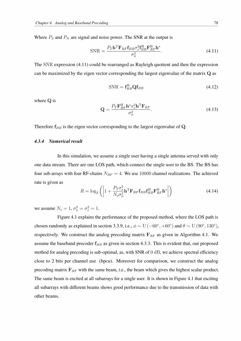
4.3.4 Numerical result

In this simulation, we assume a single user having a single antenna served with only

one data stream. There are one LOS path, which connect the single user to the BS. The BS has

four sub-arrays with four RF-chains NRF = 4. We use 10000 channel realizations. The achieved

rate is given as

R = log2

(∣∣∣∣1 +PTσ

2s

Nsσ2n

hTFRF fBBfHBBFH

RFh∗∣∣∣∣) (4.14)

we assume Ns = 1, σ2n = σ2

s = 1.

Figure 4.1 explains the performance of the proposed method, where the LOS path is

chosen randomly as explained in section 3.3.9, i.e., φ ∼ U (−60◦,+60◦) and θ ∼ U (90◦, 130◦),

respectively. We construct the analog precoding matrix FRF as given in Algorithm 4.1. We

assume the baseband precoder fBB as given in section 4.3.3. This is evident that, our proposed

method for analog precoding is sub-optimal, as, with SNR of 0 dB, we achieve spectral efficiency

close to 2 bits per channel use (bpcu). Moreover for comparison, we construct the analog

precoding matrix FRF with the same beam, i.e., the beam which gives the highest scalar product.

The same beam is excited at all subarrays for a single user. It is shown in Figure 4.1 that exciting

all subarrays with different beams shows good performance due to the transmission of data with

other beams.


-40 -20 0 20 40

SNR (dB)

0

2

4

6

8

10

12

14

Figure 4.1 – Average spectral efficiency of the proposed hybrid analog and digital precoder.

4.4 Single-cell, MU-MISO

In this section, we design the analog and digital baseband precoder for a multiuser

scenario, where each user is equipped with a single antenna. There are K users and each user

has a single LOS path. The BS is equipped with two-dimensional subarrays all have the same

orientations, excited by combination of BMs termed as PCBMS approach with N = M ×NRF

antennas assuming Ns = NRF = K, where Ns represents the number of data streams.

4.4.1 System Model

In the downlink scenario, the BS transmits the hybrid beamformed signals to all the

users K simultaneously. The received signal vector at all users is expressed as y ∈ CK×1

y =√PTHTFRFFBBs + n, (4.15)

where FRF ∈ CN×NRF is the analog precoding matrix, FBB ∈ CNRF×Ns s ∈ CNs×1, Ns =

K = NRF is the transmit signal vector satisfying E[ssH]

= σ2sIK and n is the complex noise

vector with each entry zero mean and σ2n variance as E

[nnH

]= σ2

nIK . We assume the signals

for different users are independent of each other and of the receiver noise. The channel matrix

H ∈ CN×K for all the K users is constructed as

H = [h1, . . . ,hK ] ∈ CN×K (4.16)


where hk, k = 1, . . . , K is the channel of k-th user, given as

hk =

h1k

h2k

...

hZk

∈ CN×1, (4.17)

where hzk is the channel for each sub-array and is given as

hzk = γkejϕzk︸︷︷︸

complex-path gain

ak(φ, θ) ∈ CM×1 (4.18)

where z = 1, . . . , Z, Z = NRF . γk is the amplitude for LOS path of the kth user to every subarray.

ϕzk is the phase of the LOS path of the kth user and different for each z-sub-array respectively.

ak(φ, θ) is the two-dimensional channel steering vector of the LOS path of the kth user.

The received signal yk for the kth user, which contains the target signal, interference

from the other (K − 1) users and noise is,

yk =√PThT

kFRF fkBBsk +K∑j=1j 6=k

√PThT

kFRF f jBBsj + nk (4.19)

where fkBB ∈ CNRF×1 is the kth column vector of FBB ∈ CNRF×Ns . The received signal-to-

interference and noise ratio (SINR) for the kth user can be written as

SINRk =PThT

kFRF fkBBσ2s,kf

kHBBFH

RFh∗kK∑j=1j 6=k

PThTkFRF f jBBσ

2s,jf

jHBBFH

RFh∗k + σ2n

(4.20)

The SINR (4.20) expression is derived in Appendix C.1, this can be further re-written as

SINRk =PTK

∣∣hTkFRF fkBB

∣∣2K∑j=1j 6=k

PTK

∣∣hTkFRF f jBB

∣∣2 + σ2n

(4.21)

where σs,k = 1K

. By assuming Gaussian input, the achievable sum-rate of all the K users can be

written as

R =K∑k=1

log2 (1 + SINRk) . (4.22)

4.4.2 Analog Precoder Design

To select the best possible beams in the analog precoding matrix FRF , an exhaustive

search method can be used as given in [63]. In our single cell, multi-user scenario, each of the


Algorithm 4.2: Analog precoder construction for multi-user case.1 Require: FRF (4.5)2 FRF = Block diagonal empty matrix3 for k = 1 to NRF do4 ck = γkak(φ, θ)5 pk = cH

k [w1(δp, νq), . . . ,wM(δp, νq)]

6 j = maxi

(∣∣[pk]i∣∣)7 wk(δp, νq) = wj(δp, νq)8 place the beam wk(δp, νq) in the FRF matrix (4.5)9 end

10 Return FRF

NRF chains will be assigned a beam from the M fixed beams, formed as the Kronecker product

of DFT vectors. In the exhaustive search method, MNRF are the total combinations of beams as

explained in [63], where we get the optimal combination that maximizes the spectral efficiency

R. However, it is highly time inefficient, as it becomes an infeasible solution, either by increasing

NRF or increasing M . In our proposed method, the analog precoder is designed by choosing

NRF beamforming vectors, one for each user from the set of M fixed beams. Furthermore, each

user will be served by one subarray only. We test the channel vector of each user with every

beamforming vector and select that beamforming vector, which provides the largest magnitude

of the scalar product as shown in Algorithm 4.2

4.4.3 Baseband Precoder Design

To maximize the channel capacity or sum-rate of all the K single-antenna users,

we used an iteratively WMMSE approach. We further extend the algorithm to the sum-utility

maximization problem as discussed in [64].

Consider a single cell, simultaneously transmit signals to a group of k = 1, . . . , K single antenna

users. The problem of interest is to find the digital baseband precoder FBB ∈ CNRF×Ns assuming

the sub-optimal analog precoder FRF ∈ CN×NRF fixed, such that a certain utility of the system

is maximized by respecting the power budget of the transmitter as given

K∑k=1

tr{fkBBfkH

BB

}≤ PT (4.23)

where PT is the total transmit power budget. Rewriting all the K digital baseband precoding

vectors fkBB in a matrix form as

FBB =[f1BB, . . . , f

KBB

]∈ CNRF×Ns (4.24)


4.4.3.1 Weighted Sum-Rate Maximization and a Weighted Sum-MSE Minimization

A popular utility maximization is the weighted sum-rate maximization, which is

represented as

FoptBB = arg max

FBB

K∑k=1

βkRk (4.25a)

subject to FRF ∈ wm(δp, νq),m = 0, . . . ,M − 1 (4.25b)

subject to tr{FBBFH

BB

}≤ PT (4.25c)

where the weight βk is the priority of kth user on the system and Rk is rate of the kth user. The

sum-rate for the kth user is given as,

Rk = log2

1 + PThTkFRF fkBBσ

2s,kf

kHBBFH

RFh∗k

K∑j=1j 6=k

PThTkFRF f jBBσ

2s,jf

jHBBFH

RFh∗k + σ2n

−1 .

(4.26)

Another popular utility maximization problem for MIMO-broadcast channel (BC) is the sum

MSE-minimization. Using the independence assumption of sk and nk, the MSE for kth user ekassuming yk = sk is represented as

ek = E[(sk − sk) (sk − sk)H

](4.27)

ek =(

1−√PThT

kFRF fkBBσs,k

)(1−

√PThT

kFRF fkBBσs,k

)H

+K∑j=1j 6=k

PThTkFRF f jBBσ

2s,jf

jHBBFH

RFh∗k + σ2n,k (4.28)

and therefore the sum-minimization problem can be written as

foptBB = arg min

fBB

K∑k=1

ek (4.29a)

subject to tr{FBBFH

BB

}≤ PT . (4.29b)

The expressions for ek (4.27) are derived in Appendix C.2. Now computing the Lagrangian for

this problem as

L (λ,FBB) =K∑k=1

ek + λ

(K∑k=1

tr{fkBBfkH

BB

}− PT

)(4.30)


where λ is the Lagrangian multiplier for all single antenna users. Let us now use the Karush-

Kuhn-Tucker (KKT) conditions.

∂L (λ,FBB)

∂λ=

K∑k=1

tr{fkBBfkH

BB

}− PT = 0. (4.31)

To establish equivalence between weighted sum-rate maximization and weighted sum-MSE

minimization as mentioned in [64, 65], let w′k > 0 be a scalar weight for kth user, then the

problem boils down to

arg minw′,fBB

K∑k=1

βk (w′kek − logw′k) (4.32a)

subject toK∑k=1

tr{fkBBfkH

BB

}≤ PT (4.32b)

The problem (4.32a), weighted sum-MSE minimization establishes the equivalence between

the weighted sum-rate maximization (4.25a), in a sense that the global solution fkBB for the two

problems are identical [64].

Now by fixing the baseband precoder for the kth user fkBB , the objective function (4.32a) is convex

with respect to w′k. Therefore, by checking the first order optimality condition for w′k, we can

obtain w′optk . Consider the Lagrangian function

L (w′, λ) =K∑k=1

βk (w′kek − logw′k) + λ

(K∑k=1

tr{fkBBfkH

BB

}− PT

)(4.33)

where weight vector w′ for all K users can be written as

w′ = [w′1, . . . , w′K ]

T, (4.34)

now computing ∂L(w′,λ)∂w′

k

∂L (w′, λ)

∂w′k= βk

(ek − w′−1

k

)= 0 (4.35)

ek = w′−1k (4.36)

w′optk = e−1

k . (4.37)

where ek is the mean square estimation error and w′k is a positive weight variable. The equiv-

alence relation simply implies that maximizing sum-rate can be achieved via weighted MSE

minimization.


Algorithm 4.3: Baseband precoder design using HBF-WMMSE approach (PseudoCode).1 Require: FRF (4.5)2 Initialize f lBB randomly3 J is the maximum number of iterations for convergence4 for j = 1 to J do5 Calculate w′(j)k = 1/e

(j−1)k (4.28)

6 Calculate fl(j)BB (4.38)

7 end8 Return f lopt

BB

4.4.3.2 HBF-WMMSE for sum-utility maximization

In this section, we exploit the equivalence relation discussed in section 4.4.3.1 to

derive a simple HBF-WMMSE algorithm for sum-utility maximization problem. Since, the cost

function in (4.32a) is convex given the optimization variables w′, fBB . We use block coordinate

descent (BCD) method to solve (4.32a) as given in [64]. We therefore, minimize the weighted

sum-MSE cost function by sequentially fixing one variable out of two variables, i.e., w′,FBB

and updating the second. To update the w′k variable, (4.37) is used in the closed form. To update

fkBB we use the following expression

f loptBB =

[K∑k=1

βkw′kPTFH

RFh∗khTkFRF + λIK

]−1

βlw′l

√PTFH

RFh∗l , l = 1, . . . , K. (4.38)

Where λ is designed for single cell [65] as

λ =tr {W′}PT

(4.39)

where W′ = diag {w′1, . . . , w′K}. The (4.38) is derived in Appendix C.3. The proposed HBF-

WMMSE algorithm for the designing of baseband precoder is given in Algorithm 4.3.


In this section, we present numerical results to evaluate the performance of the

proposed HBF-WMMSE algorithm using MU-MISO scenario. The proposed HBF-WMMSE

algorithm is compared with classical HBF-MMSE, HBF-ZF and HBF-MF [66, 67]. We assume

geometric channel model [47] by employing PCBMS method at BS having URA with N =

NRF ×M = 64. Each subarray has M = 16 antenna elements placed in a squared shape, i.e.,

4 × 4. There are K = 4 single antenna users with only LOS paths, and always served by one


subarray, i.e., K = NRF . The AoD azimuth φk and elevation θk for LOS path, assuming one

sector of a cell as φk ∼ U (−60◦,+60◦) and θk ∼ U (90◦, 130◦), respectively. γk for LOS is

assumed as 1 and ϕk i.e, is the phase of the complex-path gain which is uniformly generated as

ϕk ∼ U (0, 2π). Note, that in PCAPS/PCBMS network, every sub-array has the same magnitude

γk but different phase ϕzk. The noise variance is assumed as σ2n = 1. The weight for the kth user

is assumed as βk = 1.

Figure 4.2 shows the convergence of the proposed HBF-WMMSE algorithm, since

the HBF-WMMSE approach can only converge to local optimum solution, hence, its performance

depends on the starting initialization. As our problem is a two-layer optimization, so optimizing

analog beamforming matrix FRF before baseband precoding matrix FBB can help in faster

convergence. The HBF-WMMSE took 3-4 iterations for convergence.

1 2 3 4 5 6 7 8 9 10

Iterations

1

1.2

1.4

1.6

1.8

2

2.2

2.4

2.6

2.8

3

Figure 4.2 – Convergence of the HBF-WMMSE approach.

Next, we analyze the MU-MISO system, where each user has a single antenna. The overall

channel matrix of all users will always be a full rank matrix and the rank will be equal to the

number of users as K = NRF = Ns, where each user is served with one data stream. Hence,

the full capacity of the channel is always exploited. As in MISO case, the baseband precoder is

designed using HBF-WMMSE without MMSE receiver unlike mentioned in [64, 65], which as a

result, ends with a degradation in performance as compared to HBF-MMSE method [66, 67] as

shown in Figure 4.3. Note that, in this comparison, the analog precoder is the same for every


method, only the digital baseband precoder is designed differently.

-5 0 5 10 15 20 25 30 35 40

SNR (dB)

0

5

10

15

20

25

Figure 4.3 – Sum-rate performance comparison for different algorithms as compared toHBF-WMMSE method for MISO system.

Furthermore, in comparison with the FCAPS approach based analog and baseband

precoding, it is obvious that FCAPS approach will show improved performance in terms of

spectral efficiency due to the formation of narrow beams but degraded performance in terms of

energy efficiency.

87

5 CONCLUSION AND PERSPECTIVES

The next generation of wireless communication systems promises high data rates

for the end-users. One way, to make it possible is the introduction of large antenna arrays with

mmWaves, which on the side will facilitate the deployment of large antennas but will also provide

more bandwidth. The large bandwidth combined with a large number of antenna elements only at

the BS poses a challenge of the hardware implementation of such a system, therefore in addition

to spectral efficiency, energy efficiency becomes an important design objective. The large scale

antenna arrays have multiple engineering challenges including channel estimation. To tackle

these important issues, we proposed channel parameter estimation based on BM for ULA and

BMs for URA, assuming both frequency flat and selective channels. Finally, based on the this

energy efficient setup, a two-step hybrid precoding is proposed.

Specific conclusion of each chapters are given below:

• The channel parameter estimation mentioned in Chapter 2 is based on BM for

exciting ULA both for frequency flat and selective channel is discussed. An

ML based algorithm is proposed for parameter estimation assuming flat-fading

channels. In the second part of the chapter, a two-stage estimation algorithm is

proposed to obtain ML estimates of the parameters assuming frequency selective

channels. In the first stage, PREIDG algorithm is used for coarse estimation of

parameters, which are used to initialize the SAGE algorithm to further refine the

estimates. CRLB is derived to assess the performance of ML estimates.

• Chapter 3 is the extension to the two-dimensional channel parameter estimation

for frequency selective channels, where an URA is excited using multiple BMs.

A two-stage algorithm is proposed to obtain the high-resolution estimates of

the parameters. In the first-stage modified PREIDG is proposed to achieve the

coarse estimates, which is used to initialize the SAGE algorithm to obtain the

high-resolution channel parameter estimates with few iterations.

• Chapter 4 discusses the analog and baseband precoding algorithm for single

cell, SU-MISO, and MU-MISO system. On one-hand, the BMs facilitate the

energy efficient hardware implementation but on the other-side it pose a challenge

on improving the overall spectral efficiency. We proposed a two-stage hybrid

precoding algorithm, where in the first stage an analog precoding algorithm is

designed, which is then used in the second stage for the designing of the baseband

88

precoder using HBF-WMMSE.

Future research

As far as future perspectives are concerned, the following are some suggested research

lines:

• We can deploy multiple antennas at UE assuming ULA and URA to estimate AoA for

frequency selective channels.

• The BS can deploy dual polarized antennas to introduce another degree of freedom.

• The hybrid precoding, we proposed is a two-stage approach, one way which might be

investigated is to jointly optimize the analog and baseband precoding. The extension to the

multi-cell scenario would be welcome.

89

REFERENCES

1 PI, Z.; KHAN, F. An introduction to Millimeter-Wave mobile broadband systems. IEEECommunications Magazine, v. 49, n. 6, p. 101–107, June 2011. ISSN 0163-6804.

2 RAPPAPORT, T. S. et al. Millimeter wave mobile communications for 5G cellular: It willwork! IEEE Access, v. 1, p. 335–349, 2013. ISSN 2169-3536.

3 RUSEK, F. et al. Scaling up MIMO: Opportunities and challenges with very large arrays.IEEE Signal Processing Magazine, v. 30, n. 1, p. 40–60, Jan 2013. ISSN 1053-5888.

4 MO, J.; HEATH, R. W. Capacity analysis of one-bit quantized MIMO systems with transmitterchannel state information. IEEE Transactions on Signal Processing, v. 63, n. 20, p. 5498–5512,Oct 2015. ISSN 1053-587X.

5 Mezghani, A.; Nossek, J. A. On Ultra-Wideband MIMO Systems with 1-bit Quantized Outputs:Performance Analysis and Input Optimization. In: IEEE INTERNATIONAL SYMPOSIUM ONINFORMATION THEORY, 2007, Nice, France. Proceedings... Nice, France: IEEE, 2007. p.1286–1289.

6 Mezghani, A.; Nossek, J. A. Analysis of Rayleigh-fading channels with 1-bit quantized output.In: IEEE INTERNATIONAL SYMPOSIUM ON INFORMATION THEORY, 2008, Toronto,Canada. Proceedings... Toronto, Canada: IEEE, 2008. p. 260–264.

7 LEE, C.; CHUNG, W. Hybrid RF-baseband precoding for cooperative multiuser massiveMIMO systems with limited RF chains. IEEE Transactions on Communications, v. 65, n. 4,p. 1575–1589, April 2017. ISSN 0090-6778.

8 ZHU, J.; XU, W.; WANG, N. Secure massive MIMO systems with limited RF chains. IEEETransactions on Vehicular Technology, v. 66, n. 6, p. 5455–5460, June 2017. ISSN 0018-9545.

9 YANG, L.; ZENG, Y.; ZHANG, R. Efficient channel estimation for Millimeter Wave MIMOwith limited RF chains. In: IEEE INTERNATIONAL CONFERENCE ON COMMUNICA-TIONS, 2016, Kuala Lumpur, Malaysia. Proceedings... Kuala Lumpur, Malaysia: IEEE, 2016.p. 1–6.

10 LIAN, L.; LIU, A.; LAU, V. K. N. Optimal-Tuned Weighted LASSO for Massive MIMOChannel Estimation with Limited RF Chains. In: IEEE GLOBAL COMMUNICATIONS CON-FERENCE, 2017, Singapore, Singapore. Proceedings... Singapore, Singapore: IEEE, 2017.p. 1–6.

11 Moulder, W. F.; Khalil, W.; Volakis, J. L. 60-GHz Two-Dimensionally Scanning Array Em-ploying Wideband Planar Switched Beam Network. IEEE Antennas and Wireless PropagationLetters, v. 9, p. 818–821, 2010.

12 Wang, X. et al. MIMO Antenna Array System with Integrated 16x16 Butler Matrix andPower Amplifiers for 28GHz Wireless Communication. In: 12TH GERMAN MICROWAVECONFERENCE (GEMIC), 12., 2019, Stuttgart, Germany. Proceedings... Stuttgart, Germany:IEEE, 2019. p. 127–130.

13 Wang, X. et al. 28 GHz Multi-Beam Antenna Array based on Wideband High-dimension16x16 Butler Matrix. In: 13TH EUROPEAN CONFERENCE ON ANTENNAS AND PROPA-GATION (EUCAP), 13., 2019, Krakow, Poland. Proceedings... Krakow, Poland: IEEE, 2019.p. 1–4.

90

14 Wang, Y.; Ma, K.; Jian, Z. A low-loss butler matrix using patch element and honeycombconcept on SISL platform. IEEE Transactions on Microwave Theory and Techniques, v. 66,n. 8, p. 3622–3631, 2018.

15 Rodriguez-Fernandez, J. et al. Frequency-Domain Compressive Channel Estimation forFrequency-Selective Hybrid Millimeter Wave MIMO Systems. IEEE Transactions on WirelessCommunications, v. 17, n. 5, p. 2946–2960, 2018.

16 Wang, B. et al. Spatial and Frequency-Wideband Effects in Millimeter-Wave Massive MIMOSystems. IEEE Transactions on Signal Processing, v. 66, n. 13, p. 3393–3406, 2018.

17 Wang, B. et al. Spatial-Wideband Effect in Massive MIMO with Application in mmWaveSystems. IEEE Communications Magazine, v. 56, n. 12, p. 134–141, 2018.

18 GURBUZ, A. C.; YAPICI, Y.; GUVENC, I. Sparse Channel Estimation in Millimeter-WaveCommunications via Parameter Perturbed OMP. In: IEEE INTERNATIONAL CONFERENCEON COMMUNICATIONS WORKSHOPS (ICC WORKSHOPS), 13., 2018, Kansas, USA.Proceedings... Kansas, USA: IEEE, 2018. p. 1–6.

19 HE, K.; LI, Y.; YIN, C. A novel CS-based non-orthogonal multiple access MIMO systemfor downlink of MTC in 5G. In: IEEE 28TH ANNUAL INTERNATIONAL SYMPOSIUM ONPERSONAL, INDOOR, AND MOBILE RADIO COMMUNICATIONS (PIMRC), 13., 2017,Montreal, Canada. Proceedings... Montreal, Canada: IEEE, 2017. p. 1–5.

20 WANG, P. et al. Sparse channel estimation in millimeter wave communications: Exploitingjoint AoD-AoA angular spread. In: 2017 IEEE INTERNATIONAL CONFERENCE ON COM-MUNICATIONS (ICC), 13., 2017, Paris, France. Proceedings... Paris, France: IEEE, 2017.p. 1–6.

21 ELDAR, Y. C.; KUPPINGER, P.; BoLCSKEI, H. Block-sparse signals: Uncertainty relationsand efficient recovery. IEEE Transactions on Signal Processing, v. 58, n. 6, p. 3042–3054,June 2010. ISSN 1053-587X.

22 ALKHATEEB, A. et al. Channel estimation and hybrid precoding for millimeter wavecellular systems. IEEE Journal of Selected Topics in Signal Processing, v. 8, n. 5, p. 831–846,Oct 2014. ISSN 1932-4553.

23 LEE, J.; GIL, G.; LEE, Y. H. Channel estimation via orthogonal matching pursuit for hybridMIMO systems in millimeter wave communications. IEEE Transactions on Communications,v. 64, n. 6, p. 2370–2386, June 2016. ISSN 0090-6778.

24 Venugopal, K. et al. Channel estimation for hybrid architecture-based wideband millimeterwave systems. IEEE Journal on Selected Areas in Communications, v. 35, n. 9, p. 1996–2009,Sep. 2017. ISSN 1558-0008.

25 SHAHMANSOORI, A. et al. Position and orientation estimation through millimeter-waveMIMO in 5G systems. IEEE Transactions on Wireless Communications, v. 17, n. 3, p. 1822–1835, March 2018. ISSN 1536-1276.

26 ZHU, D.; CHOI, J.; HEATH, R. W. Auxiliary beam pair design in mmwave cellular sys-tems with hybrid precoding and limited feedback. In: INTERNATIONAL CONFERENCE ONACOUSTICS, SPEECH AND SIGNAL PROCESSING (ICASSP), 41., 2016, Shanghai, China.Proceedings... Shanghai, China: IEEE, 2016. p. 7849–7853.

91

27 ZHU, D.; CHOI, J.; HEATH, R. W. Two-dimensional AoD and AoA acquisition for wide-band millimeter-wave systems with dual-polarized MIMO. IEEE Transactions on WirelessCommunications, v. 16, n. 12, p. 7890–7905, Dec 2017. ISSN 1536-1276.

28 Singh, J.; Ramakrishna, S. On the Feasibility of Codebook-Based Beamforming in MillimeterWave Systems With Multiple Antenna Arrays. IEEE Transactions on Wireless Communica-tions, v. 14, n. 5, p. 2670–2683, 2015.

29 Hu, C. et al. Super-Resolution Channel Estimation for MmWave Massive MIMO WithHybrid Precoding. IEEE Transactions on Vehicular Technology, v. 67, n. 9, p. 8954–8958,2018.

30 Ma, W.; Qi, C.; Li, G. Y. High-resolution channel estimation for frequency-selective mmwavemassive mimo systems. IEEE Transactions on Wireless Communications, v. 19, n. 5, p. 3517–3529, 2020.

31 Sommerkorn, G. et al. Reduction of DoA estimation errors caused by antenna array imper-fections. In: 29TH EUROPEAN MICROWAVE CONFERENCE, 13., 1999, Munich, Germany.Proceedings... Munich, Germany: IEEE, 1999. p. 287–290.

32 EBERHARDT, M.; ESCHLWECH, P.; BIEBL, E. Investigations on antenna array calibrationalgorithms for direction-of-arrival estimation. Advances in Radio Science, v. 14, p. 181–190,2016. Disponıvel em: 〈https://www.adv-radio-sci.net/14/181/2016/〉.

33 Xuefeng Yin; Fleury, B. H. Nominal direction and direction spread estimation for slightlydistributed scatterers using the SAGE algorithm. In: IEEE 61ST VEHICULAR TECHNOLOGYCONFERENCE, 61., 2005, Stockholm, Sweden. Proceedings... Stockholm, Sweden: IEEE,2005. p. 25–29.

34 Feng, R. et al. Wireless channel parameter estimation algorithms: Recent advances andfuture challenges. China Communications, v. 15, n. 5, p. 211–228, 2018.

35 de Leon, F. A.; Marciano, J. J. S. Application of MUSIC, ESPRIT and SAGE Algorithmsfor Narrowband Signal Detection and Localization. In: TENCON 2006 - 2006 IEEE REGION10 CONFERENCE, 61., 2006, Hong Kong, China. Proceedings... Hong Kong, China: IEEE,2006. p. 25–29.

36 Tschudin, M. et al. Comparison between unitary ESPRIT and SAGE for 3-D channel sound-ing. In: IEEE 49TH VEHICULAR TECHNOLOGY CONFERENCE (CAT. NO.99CH36363),49., 1999, Houston, USA. Proceedings... Houston, USA: IEEE, 1999. p. 1324–1329.

37 Feng, R. et al. Comparison of music, unitary ESPRIT, and SAGE algorithms for estimat-ing 3D angles in wireless channels. In: IEEE/CIC INTERNATIONAL CONFERENCE ONCOMMUNICATIONS IN CHINA (ICCC), 49., 2017, Qingdao, China. Proceedings... Qingdao,China: IEEE, 2017. p. 1–5.

38 Ayach, O. E. et al. Spatially Sparse Precoding in Millimeter Wave MIMO Systems. IEEETransactions on Wireless Communications, v. 13, n. 3, p. 1499–1513, 2014.

39 Mendez-Rial, R. et al. Hybrid MIMO Architectures for Millimeter Wave Communications:Phase Shifters or Switches? IEEE Access, v. 4, p. 247–267, 2016.

https://www.adv-radio-sci.net/14/181/2016/

92

40 Zeng, Y.; Zhang, R.; Chen, Z. N. Electromagnetic Lens-Focusing Antenna Enabled MassiveMIMO: Performance Improvement and Cost Reduction. IEEE Journal on Selected Areas inCommunications, v. 32, n. 6, p. 1194–1206, 2014.

41 Lin, T. et al. Hybrid Beamforming for Millimeter Wave Systems Using the MMSE Criterion.IEEE Transactions on Communications, v. 67, n. 5, p. 3693–3708, 2019.

42 Ardah, K. et al. Hybrid Analog-Digital Beamforming Design for SE and EE Maximizationin Massive MIMO Networks. IEEE Transactions on Vehicular Technology, v. 69, n. 1, p.377–389, 2020.

43 Ribeiro, L. N. et al. Energy Efficiency of mmWave Massive MIMO Precoding With Low-Resolution DACs. IEEE Journal of Selected Topics in Signal Processing, v. 12, n. 2, p. 298–312, 2018.

44 Nguyen, D. H. N. et al. Hybrid MMSE Precoding and Combining Designs for mmWaveMultiuser Systems. IEEE Access, v. 5, p. 19167–19181, 2017.

45 Garcia-Rodriguez, A. et al. Hybrid analog digital precoding revisited under realistic RFmodeling. IEEE Wireless Communications Letters, v. 5, n. 5, p. 528–531, 2016.

46 S.M.KAY. Fundamentals of Statistical Signal processing: Estimation Theory. [S.l.]:New York, NY, USA: prentice-Hall, 1993, 1993.

47 SAMIMI, M. K.; RAPPAPORT, T. S. 3-D millimeter-wave statistical channel model for5G wireless system design. IEEE Transactions on Microwave Theory and Techniques, v. 64,n. 7, p. 2207–2225, July 2016. ISSN 0018-9480.

48 Jost, T. et al. Detection and tracking of mobile propagation channel paths. IEEE Transac-tions on Antennas and Propagation, v. 60, n. 10, p. 4875–4883, 2012.

49 FLEURY, B. et al. Channel parameter estimation in mobile radio environments using theSAGE algorithm. IEEE Journal on Selected Areas in Communications, v. 17, n. 3, p. 434–450,March 1999. ISSN 0733-8716.

50 Asim, F. et al. Maximum likelihood channel estimation for Millimeter-Wave MIMO systemswith hybrid beamforming. In: IEEE 23RD INTERNATIONAL ITG WORKSHOP ON SMARTANTENNAS, 2019, Vienna, Austria. Proceedings... Vienna, Austria: IEEE, 2019. p. 1–6.

51 Asim, F. et al. Channel parameter estimation for millimeter-wave cellular systems withhybrid beamforming. Signal Processing, v. 176, p. 2619–2692, July 2020. ISSN 0165-1684.

52 Baggen, L.; Bottcher, M.; Eube, M. 3D-Butler matrix topologies for phased arrays. In:INTERNATIONAL CONFERENCE ON ELECTROMAGNETICS IN ADVANCED APPLICA-TIONS, 41., 2007, Torino, Italy. Proceedings... Torino, Italy: IEEE, 2007. p. 531–534.

53 FRANK, R. L.; ZADOFF, S. A. Phase shift pulse codes with good periodic correlationproperties (correspondence). IRE Trans. on Information Theory, v. 8, p. 381–382, Oct 1962.

54 POPOVIC, B. M. Generalized chirp-like polyphase sequences with optimum correlationproperties. IEEE Transactions on Information Theory, v. 38, n. 4, p. 1406–1409, Jul 1992.ISSN 0018-9448.

93

55 ROHRS, U. H.; LINDE, L. P. Some unique properties and applications of perfect squaresminimum phase CAZAC sequences. In: IEEE 1992 SOUTH AFRICAN SYMPOSIUM ON COM-MUNICATIONS AND SIGNAL PROCESSING, 1992, Cape Town, South Africa. Proceedings...Cape Town, South Africa: IEEE, 1992. p. 155–160.

56 Zoltowski, M. D.; Haardt, M.; Mathews, C. P. Closed-form 2-d angle estimation withrectangular arrays in element space or beamspace via unitary esprit. IEEE Transactions onSignal Processing, v. 44, n. 2, p. 316–328, 1996.

57 Zhang, J.; Haardt, M. Channel estimation for hybrid multi-carrier mmwave MIMO systemsusing three-dimensional unitary esprit in DFT beamspace. In: IEEE 7TH INTERNATIONALWORKSHOP ON COMPUTATIONAL ADVANCES IN MULTI-SENSOR ADAPTIVE PRO-CESSING (CAMSAP), 2017, Curacao, Netherlands Antilles. Proceedings... Curacao, Nether-lands Antilles: IEEE, 2017. p. 1–5.

58 Rakhimov, D. et al. Channel Estimation for Hybrid Multi-Carrier mmWave MIMO SystemsUsing 3-D Unitary Tensor-ESPRIT in DFT beamspace. In: IEEE 53RD ASILOMAR CONFER-ENCE ON SIGNALS, SYSTEMS, AND COMPUTERS, 53., 2019, Pacific Grove CA, USA.Proceedings... Pacific Grove CA, USA: IEEE, 2019. p. 447–451.

59 Fessler, J. A.; Hero, A. O. Space-alternating generalized expectation-maximization algorithm.IEEE Transactions on Signal Processing, v. 42, n. 10, p. 2664–2677, 1994.

60 Amadori, P. V.; Masouros, C. Interference-driven antenna selection for massive multiusermimo. IEEE Transactions on Vehicular Technology, v. 65, n. 8, p. 5944–5958, Aug 2016.ISSN 1939-9359.

61 Gholam, F.; Via, J.; Santamaria, I. Beamforming design for simplified analog antennacombining architectures. IEEE Transactions on Vehicular Technology, v. 60, n. 5, p. 2373–2378, Jun 2011. ISSN 1939-9359.

62 Venkateswaran, V.; van der Veen, A. Analog beamforming in mimo communications withphase shift networks and online channel estimation. IEEE Transactions on Signal Processing,v. 58, n. 8, p. 4131–4143, Aug 2010. ISSN 1941-0476.

63 Han, Y. et al. Dft-based hybrid beamforming multiuser systems: Rate analysis and beamselection. IEEE Journal of Selected Topics in Signal Processing, v. 12, n. 3, p. 514–528, June2018. ISSN 1941-0484.

64 Shi, Q. et al. An Iteratively Weighted MMSE Approach to Distributed Sum-Utility Maxi-mization for a MIMO Interfering Broadcast Channel. IEEE Transactions on Signal Processing,v. 59, n. 9, p. 4331–4340, 2011.

65 Christensen, S. S. et al. Weighted sum-rate maximization using weighted mmse for mimo-bc beamforming design. IEEE Transactions on Wireless Communications, v. 7, n. 12, p.4792–4799, 2008.

66 Li, A.; Masouros, C. Hybrid precoding and combining design for millimeter-wave multi-userMIMO based on SVD. In: IEEE INTERNATIONAL CONFERENCE ON COMMUNICATIONS(ICC), 2017, Paris, France. Proceedings... Paris, France: IEEE, 2017. p. 1–6.

67 Joham, M. et al. Transmit Wiener filter for the downlink of TDDDS-CDMA systems. In:IEEE SEVENTH INTERNATIONAL SYMPOSIUM ON SPREAD SPECTRUM TECHNIQUES

94

AND APPLICATIONS, 2002, Prague, Czech Republic. Proceedings... Prague, Czech Republic:IEEE, 2002. p. 1–5.

68 PAPOULIS, A.; PILLAI, S. U. Probability, Random Variables, and Stochastic Processes.[S.l.]: McGraw Hill, 2002.

69 H.V.POOR. An Introduction to Signal Detection and Estimation . [S.l.]: Springer Verlagt,1994.

70 DIETRICH, F. A. A Tutorial on Channel Estimation with SAGE . [S.l.]: Technical ReportTUM-LNS-TR-06-03, 2006.

71 MCLACHLAN, G. J.; KRISHNAN, T. The EM Algorithm and Extensions. . [S.l.]: JohnWiley and Sons, Inc., New York, 1997.

95

APPENDICES

96

APPENDIX A – ML Estimation and CRLB

We derive the ML estimate for different parameters assuming frequency flat fading

channel. We further derive configuration of the SAGE to get the ML estimates of the channel

parameters assuming frequency selective channel. We also derive the CRLB to assess the

performance of the ML estimates.

A.1 Maximum Likelihood estimation for frequency flat fading channel

Let us assume a random variable Y which has a multivariate complex Gaussian pdf

parameterized by the parameter vector η and assuming L = M ,

L(Y;η) =1

πM2 det Rexp

(−vec

{Y −

√PTαA(µ)C

}H

R−1 vec{

Y −√PTαA(µ)C

})(A.1)

where η

η = [σ2n,√PTα, µ]T (A.2)

and further assuming spatiality and temporally uncorrelated noise entries ends with the noise

variance matrix R


]= σ2

nIM2 . (A.3)

Now take natural logarithm on both sides of (A.1) as 1

`(Y,η) = loge(L(Y;η)) = −M2(loge(π) + loge(σ

2n))− 1

σ2n

tr {(Y−√PT α A(µ)C

)(Y −

√PT α A(µ)C

)H}

(A.4)

The ML estimator can be given as

η = arg maxη{`(Y,η)} . (A.5)

Now differentiating (A.4) with respect to σ2n and equating it to zero

∂`(Y,η)

∂σ2n

= −M2

σ2n

+1

σ4n

tr

{(Y −

√PT α A(µ)C

)(Y −

√PT α A(µ)C

)H}

= 0 (A.6)

σ2n =

1

M2tr

{(Y −

√PT α A(µ)C

)(Y −

√PT α A(µ)C

)H}. (A.7)

1 det(cA) = cNdet(A) if A ∈ CN×N and det(IN ) = 1

APPENDIX A. ML Estimation and CRLB 97

Now plugging (A.7) into (A.4) leads to

` (Y,η) = −M2 loge(π)−M2 loge

(1

M2tr

{(Y −

√PT α A(µ)C

)(Y −

√PT α A(µ)C

)H})

−(

1

M2tr

{(Y −

√PT α A(µ)C

)(Y −

√PT α A(µ)C

)H})−1

tr

{(Y −

√PT α A(µ)C

)(Y −

√PT α A(µ)C

)H}. (A.8)

Now to maximize the ` (Y,η), we can first drop any part not depending on η,

` (Y,η) = −M2 loge

(1

M2tr

{(Y −

√PT α A(µ)C

)(Y −

√PT α A(µ)C

)H})

(A.9)

and since loge is a monotonic function, we can maximize the so called concentrated loss function

`c (Y,η) = −tr

{(Y −

√PT α A(µ)C

)(Y −

√PT α A(µ)C

)H}

(A.10)

= −tr{YYH

}+√PTαtr

{A(µ)CYH

}+√PTα

∗tr{YCHAH(µ)

}− αα∗PT tr

{A(µ)CCHA(µ)H

}. (A.11)

Now take the derivative of of `c (Y,η) (A.11) with respect to α∗

∂`c (Y,η)

∂α∗=√PT tr

{YCHAH(µ)

}− αPT tr

{A(µ)CCHA(µ)H

}= 0 (A.12)

which ends up to

ˆ(√PTα) =

tr{YCHAH(µ)

}tr {A(µ)CCHAH(µ)}

=tr{YCHAH(µ)

}Mtr {A(µ)AH(µ)}

. (A.13)

assuming CCH = M1M . Now we plug (A.13) into (A.11) and get

`c (Y,η) = −tr{YYH

}+

tr{YCHAH(µ)

}Mtr {A(µ)AH(µ)}

tr{A(µ)CYH

}+

tr{A(µ)CYH

}Mtr {A(µ)AH(µ)}

tr{A(µ)CYH

}−

tr{A(µ)CYH

}tr{YCHAH(µ)

}M2 (tr {A(µ)AH(µ)})2 Mtr

{A(µ)AH(µ)

}(A.14)

Now it ends up with

µ = arg maxµ

`c (Y,η) = arg maxµ

tr{A(µ)CYH

}tr{YCHAH(µ)

}Mtr {A(µ)AH(µ)}

(A.15)

Now we use tr{YCHAH(µ)

}= vec {A(µ)C}H vec {Y} to get

µ = arg maxµ

vec {A(µ)C}H vec {Y} vec {Y}H vec {A(µ)C}Mtr {A(µ)AH(µ)}

(A.16)


Now defining RY = vec {Y} vec {Y}H as rank-one matrix. The ratio in (A.16) is Rayleigh

quotient, which is maximized by the eigenvector of RY corresponding to the largest eigenvalue of

RY. Since RY is rank-one matrix, there is only one-non-zero eigenvalue and the corresponding

eigenvector is vec {Y}. Now let us call this eigenvector u = vec{Y} and by reformulating the

problem in (A.16) by

‖u− vec {A(µ)C}‖22 = ‖U−A(µ)C‖2

F = tr{

(U−A(µ)C) (U−A(µ)C)H}

= tr{UUH

}− tr

{A(µ)CUH

}− tr

{UCHAH(µ)

}+ tr

{A(µ)CCHAH(µ)

}.(A.17)

Now the problem (A.16) can be re-written as

µ = arg minµ‖u− vec {A(µ)C}‖2

2 (A.18)

therefore we take the derivative of (A.17) with respect to AH(µ) and equating it equal to zero

∂

∂AH(µ)

(tr{UUH

}− tr

{A(µ)CUH

}− tr

{UCHAH(µ)

}+ tr

{A(µ)CCHAH(µ)

})= 0

(A.19)

which leads to

−(UCH

)T+MAT(µ) = 0 (A.20)

MAT(µ) =(UCH

)T (A.21)

since U = unvec{u} = unvec{vec{Y}} = Y and for notational convenience A(µ) = A, then

finally

A =1

MYCH (A.22)

and in order to estimate the spatial frequency µ, we can solve this using one dimensional search

µ = arg minµ

tr{

diag(A−A(µ)

)diag

(A−A(µ)

)∗}. (A.23)

Using back substituting, µ in (A.13) to get ˆ(√PTα). Finally use µ and ˆ(

√PTα) in (A.7) to

estimate σ2n.


A.2 Derivation of the FIM F(η)

The entries of the F (η) are derive as

[F(η)]11 =PTσ2n

2Re(tr{CHAH(µ)A(µ)C

})(A.24)

[F(η)]12 =PTσ2n

2Re(tr{jCHAH(µ)A(µ)C

})(A.25)

[F(η)]13 =PTσ2n

2Re

(tr

{αCHAH(µ)

∂A(µ)

∂µC

})(A.26)

[F(η)]22 =PTσ2n

2Re(tr{CHAH(µ)A(µ)C

})(A.27)

[F(η)]23 =PTσ2n

2Re

(tr

{−j αCHAH(µ)

∂A(µ)

∂µC

})(A.28)

[F(η)]33 =PTσ2n

2Re

(tr

{|α|2CH∂AH(µ)

∂µ

∂A(µ)

∂µC

}). (A.29)

Derivative of A(µ)

The partial derivative of A(µ) is calculated as

∂A(µ)

∂µ= diag{a′H(µ)w(Φk)}M−1

k=0 (A.30)

with

a′(µ) =[0, (−j)e−jµ, . . . , (−j(M − 1))e−j(M−1)µ

]T. (A.31)

A.3 SAGE

Let us assume that the observed data Y as a random variable of the multivariate

complex Gaussian pdf denoted by pY (Y;η) parametrized by the parameter vector η can be

represented mathematically as

pY (Y;η) =1

πML det Rexp

−vec

{Y −

√PT

R∑r=1

αrA(µr)C(τr)

}H

R−1 vec

{Y −

√PT

R∑r=1

αrA(µr)C(τr)

}). (A.32)

where (.)H denotes complex conjugate transposition, det represents the determinant and R ∈

CML×ML is the temporally and spatially uncorrelated noise covariance matrix as


]= σ2

nIML (A.33)


where σ2n is the noise variance. The likelihood function L (Y;η) with respect to parameter vector

η is given as

L (Y;η) = pY (Y;η) (A.34)

The likelihood function L (Y;η) is a function of the parameter vector, estimation of which is

based on a given realization of the random variable, the matrix Y contains the samples of the

complex baseband signals at the antenna array output. The parameter vector η can be defined as

η =[√

PTαT,µT, τT

]T

. (A.35)

The ML estimator can be formed as

η = arg maxη

L (Y;η) (A.36)

(A.36) is the non-linear optimization problem and performing the global maximization directly,

consequently does not have a closed-form solution, therefore, the Expectation-Maximization

(EM) algorithm gives a sequential approximation of the problem (A.36). EM algorithm performs

a sequence of maximization steps in the space of low dimension which ends with the reduction

in complexity. But in our scenario, we use the SAGE algorithm for our scenario to solve this

non-linear problem with hardware constraints. In the SAGE algorithm, we estimate the channel

parameters sequentially unlike EM, where the parameters are estimated in parallel. This could

increase the convergence rate as we can use the current estimates from all other multipath,

consequently interference subtraction which improves the expectation E-step.

The SAGE algorithm classifies the signals into a complete but an unobservable data

X and an incomplete but an observable data Y. These two complete and incomplete data sets

have a relationship which is described by a deterministic many-to-one- mapping as

Y = f (X) (A.37)

Note that, the dimension of parameter vector, i.e., dim(η) gives the dimensionality, where ηrcontains a all the parameters present in η except those contained in ηr.

A random hidden matrix represented as Xr having a pdf p (Xr;η) is an admissible

hidden data space with respect to ηr for p (Y;η), if the joint density of Xr and Y satisfies the

following

p (Y,Xr;η) = p(Y | Xr;ηr) p(Xr;η) (A.38)


The conditional density of the observation matrix Y given the hidden matrix Xr which depends

on ηr rather than ηr which ultimately means that all information about the channel parameters

which is ηr is contained in Y which means in Xr. Furthermore, if Xr is completely known, then,

as a result, ηr is not required to be completely known to uniquely define Y. This can be prove

using

p(Y;η) = p(Y;ηr,ηr). (A.39)

Using Bayes-theorem [68] can lead to

p(Y;ηr,ηr) =p(Y | Xr;ηr) p(Xr;ηr,ηr)

p(Xr | Y;ηr,ηr), (A.40)

now taking the natural logarithm on (A.40) to get the log-likelihood function

`(Y;ηr;ηr) = `(Y | Xr;ηr) + `(Xr;ηr,ηr) − `(Xr | Y;ηr,ηr). (A.41)

As the hidden data space Xr is unobservable, the SAGE algorithm solve the problem of maximiz-

ing the log-likelihood function ` (Y;η) by iteratively and sequentially maximizing the conditional

expectation of ` (Y;η) with respect to the hidden data space Xr given the observed data Y having

the current update of the estimate of parameter vector η. Now take the conditional expectation

on both sides of (A.41) with respect to hidden data space Xr given the Y and having the current

update of the estimate of the parameter vector η leads to

EXr [`(Y;ηr,ηr | Y; η)] = EXr [`(Y | Xr;ηr) | Y; η] + EXr [`(Xr;ηr,ηr | Y; η)]

− EXr [`(Xr | Y;ηr,ηr | Y; η)] (A.42)

with

EXr [`(Y;ηr,ηr | Y; η)] = `(Y;ηr,ηr) (A.43)

As we see that the first term on the right hand side of (A.42) is independent on the vector ηr and

the third term of (A.42) can be derived as

EXr [`(Xr | Y;ηr,ηr | Y; η)]− EXr [`(Xr | Y; η) | Y; η] ≤ 0. (A.44)

Now applying Jensen’s inequality [69] to (A.44) which states that for a concave function f(x) is

given as

E[f(x)] ≤ f(E[x]), (A.45)


we can prove (A.44) by applying Jensen’s inequality as follows

= EXr

[lnL(Xr | Y;ηr,ηr)

L(Xr | Y; η)| Y; η

]≤ ln EXr

[L(Xr | Y;ηr,ηr)

L(Xr | Y; η)| Y; η

]= ln

∫Xr

L(Xr | Y;ηr,ηr)

L(Xr | Y; η)L(Xr | Y; η) dXr

= ln

∫Xr

L(Xr | Y;ηr,ηr) dXr

= ln(1) = 0. (A.46)

whereXr represents the range of Xr. To maximize (A.42), the only term EXr [`(Xr;ηr,ηr | Y; η)]

is need to be iteratively and sequentially maximized with respect to ηr. This can be affirm as

`(Y;ηr,ηr) ≥ `(Y; η) (A.47)

iff

EXr [`(Xr;ηr,ηr | Y; η)] ≥ EXr [`(Xr; η) | Y; η] . (A.48)

The complete but unobservable hidden data space is given as

X = [X1, . . . ,XR] ∈ CM×L (A.49)

given as

Y = f(X) = f ([X1, . . . ,XR]) =R∑r=1

Xr (A.50)

Xr = Sr(ηr) + Nr (A.51)

Rr = E[vec{Nr}vec{Nr}H] = βrσ2nIML (A.52)

and now the decomposition of the white noise term N

N =R∑r=1

Nr (A.53)

The noise entries of matrix Nr are temporally and spatially independent having complex Gaussian

distributed with variance βrσ2n. The variance of the noise should satisfy the following condition

R∑r=1

βr = 1. (A.54)


Now let us assume that Xr are independent with r = 1, . . . , R, we can get

`(Y;η) =R∑r=1

`(Xr;ηr)

=R∑r=1

ln

(1

(πβrσ2n)ML

exp

(−‖Xr − Sr(ηr)‖2

F

βrσ2n

))(A.55)

and

EX [`(X;η | Y; η)] =R∑r=1

EXr [`(Xr;ηr | Y; η)] . (A.56)

The parameter vector ηr which contains the parameters of the channel which parametrize one

wavefront/path and each of the R parameter vectors which determines a subset of the main

parameter vector η.

By maximizing EX [`(X;η | Y; η)], we can independently maximize each terms of

the right hand side of (A.56), as they it depends on different subsets of η. EXr [`(Xr;ηr | Y; η)]

only depends on the parameters of the r-th wavefront/path and therefore can estimate η of all

channel parameters from a previous iteration which simplifies the optimization. The terms in the

(A.56) can be written as

EXr [ln(Xr;ηr) | Y; η] = EXr [ln b(Xr) | Y; η] + cH(ηr)EXr [t(Xr) | Y; η]− ln a(ηr)

(A.57)

To estimate the parameters of one wavefront/path, we identify the pdf of the hidden data space

with the exponential family [70, 69, 71] as

p(Xr;ηr) =b(Xr)

a(ηr)exp(cH(ηr)t(Xr)) (A.58)

The different variables in (A.58) can be identified as

a(ηr) = exp

(‖vec{Sr(ηr)}‖2

2

βrσ2n

)(A.59)

b(Xr) =1

(πβrσ2n)ML

exp

(−‖vec{Xr}‖2

2

βrσ2n

)(A.60)

c(ηr) =1

βrσ2n

vec{Sr(ηr)}

vec{Sr(ηr)∗}

(A.61)

t(Xr) =

vec{Xr}

vec{Xr}∗

. (A.62)

Keep in mind that t (Xr) is a complete sufficient statistic for ηr. Now the choice of the hidden

space introduces wavefront/path by wavefront/path parameter estimation. Now in order to


maximize (A.57) iteratively and sequentially, two steps, i.e., Expectation step E-step and the

maximization step M-step are performed. The E-step would estimate the unobservable hidden

data space Xr. The E-step is actually calculating R expected values of t(Xr).

E-Step:

The expected value of the second term has to be calculated before maximizing

(A.57). It is actually, an estimator for the sufficient statistic for the parameters of the r-th

wavefront/path. Therefore, in the E-step the unobservable, complete and hidden data space is

estimated conditioned on the observed but incomplete data Y and also on the previous estimate

of the parameter vector η which is obtained in the previous iteration as

Xr = EXr [Xr | Y; η] = Sr(ηr) + βr

(Y −

R∑r′=1

Sr′(ηr′)

)(A.63)

Xr = (1− βr)Sr(ηr) + βr

Y −R∑

r′=1r′ 6=r

Sr′(ηr′)

. (A.64)

In (A.64), βr controls the rate of convergence. When βr = 0, the estimate of the hidden data space

Xr of the sufficient statistic is not updated for the r-th wavefront/path. Similarly, by choosing

βr = 1, the convergence rate is largest because of the amount of new information incorporated

into the estimate of the hidden data space Xr. The stochastic mapping from the hidden data

space Xr to the observable signal Y is given as

Y = Xr +R∑

r′=1r′ 6=r

Sr′ + Nr′ (A.65)

The sequence of the parameter vector ηr(k), k represents the number of iterations and is given

asηr(1) = [τ1]

ηr(2) = [µ1]

ηr(3) = [α1]

ηr(4) = [τ2]...

(A.66)


As discussed above, for the fast convergence rate we assume βr = 1, which leads the hidden data

space estimation as

Xr = Y −R∑

r′=1r′ 6=r

Sr′(ηr′). (A.67)

M-Step:

Using (A.57), (A.59) and (A.61) with the definition of hidden data space of Xr

(A.63), we get

ηr = arg maxηr

{(cH(ηr)EXr [t(Xr) | Y; ηr]− ln a(ηr)

)}(A.68)

cH =1

βrσ2n

[vecH{Sr(ηr)}vecT{Sr(ηr)}

](A.69)

ln a(ηr) =‖vec{Sr(ηr)}‖2

2

βrσ2n

(A.70)

EXr [t(Xr) | Y; ηr] =[vecT{Xr}vecH{Xr}

]T

(A.71)

ηr = arg maxηr

{1

βrσ2n

(tr{SH

r (ηr)Xr}+ tr{STr (ηr)X

∗r} − ‖Sr(ηr)‖2

F

)}(A.72)

The first term in right hand side of (A.57) is independent of ηr and was omitted. From (2.31)

and (A.35), we have 2

Sr(ηr) =√PTαrA(µr)C(τr), C(τr)C

H(τr) = LIM (A.73)

and with simplification

‖Sr(ηr)‖2F = tr

{SHr (ηr)Sr(ηr)

}= PTαrα

∗rtr{CH(τr)A

H(µr)A(µr)C(τr)} (A.74)

Putting the values in (A.68) will lead us to

ηr = arg maxηr

{1

βrσ2n

(√PTα

∗rtr{CH(τr)A

H(µr)Xr}+√PTαrtr{CT(τr)A

T(µr)X∗r}

−PTαrα∗rtr{CH(τr)AH(µr)A(µr)C(τr)}

)}(A.75)

= arg maxηr{Λr(ηr)}

To estimate αr, we need to derivate (A.75) and putting it equal to zero,

∂Λr(ηr)

∂α∗r=

1

βrσ2n

(√PT tr

{CH(τr)A

H(µr)Xr

}− PTαrtr{CH(τr)A

H(µr)A(µr)C(τr)})

= 0

(A.76)2 tr

(ATB

)= vec

(AT)vec (B)


Solving we can get an analytical expression

αr =tr{

CH(τr)AH(µr)Xr

}√PT tr{CH(τr)AH(µr)A(µr)C(τr)}

(A.77)

To obtain an estimator for τr and µr, put (A.77) in (A.75).

Rewriting (A.75) and solving will lead us to 3

ηr = arg maxηr

1

βrσ2n

2

∣∣∣tr{CH(τr)AH(µr)Xr

}∣∣∣2tr{CH(τr)AH(µr)A(µr)C(τr)}

−

∣∣∣tr{CH(τr)AH(µr)Xr

}∣∣∣2tr{CH(τr)AH(µr)A(µr)C(τr)}

(A.78)

(τr, µr) = arg maxτr,µr


H(µr)Xr

}∣∣∣2βrσ2


(A.79)

Steps:

The delay estimation τr can be iteratively maximized as

τr = arg maxτr


H(µr)Xr

}∣∣∣2βrσ2


, (A.80)

similarly the spatial frequency µr can be iteratively maximized as

µr = arg maxµr


H(µr)Xr

}∣∣∣2βrσ2


, (A.81)

while in the end ˆ√PTαr can be analytically found as

ˆ√PTαr =

tr{

CH(τr)AH(µr)Xr

}tr{CH(τr)AH(µr)A(µr)C(τr)}

. (A.82)

3 2Re (a) = (a+ a∗)


A.4 Derivation of the FIM F(η)

The entries of the block matrices of the FIM F(η) (2.72) are derived below,

[FRe{α}Re{α}]ij =PTσ2n

2Re

(tr

{R∑r=1

∂α∗r∂Re{αi}

CH(τr)AH(µr)

R∑r=1

∂αr∂Re{αj}

A(µr)C(τr)

})(A.83)

[FRe{α}Im{α}]ij =PTσ2n

2Re

(tr

{R∑r=1

∂α∗r∂Re{αi}

CH(τr)AH(µr)

R∑r=1

∂αr∂Im{αj}

A(µr)C(τr)

})(A.84)

[FRe{α}µ]ij =PTσ2n

2Re

(tr

{R∑r=1

∂α∗r∂Re{αi}

CH(τr)AH(µr)

R∑r=1

αr∂A(µr)

∂µjC(τr)

})(A.85)

[FRe{α}τ ]ij =PTσ2n

2Re

(tr

{R∑r=1

∂α∗r∂Re{αi}

CH(τr)AH(µr)

R∑r=1

αrA(µr)∂C(τr)

∂τj

})(A.86)

[FIm{α}Im{α}]ij =PTσ2n

2Re

(tr

{R∑r=1

∂α∗r∂Im{αi}

CH(τr)AH(µr)

R∑r=1

∂αr∂Im{αj}

A(µr)C(τr)

})(A.87)

[FIm{α}µ]ij =PTσ2n

2Re

(tr

{R∑r=1

∂α∗r∂Im{αi}

CH(τr)AH(µr)

R∑r=1

αr∂A(µr)

∂µjC(τr)

})(A.88)

[FIm{α}τ ]ij =PTσ2n

2Re

(tr

{R∑r=1

∂α∗r∂Im{αi}

CH(τr)AH(µr)

R∑r=1

αrA(µr)∂C(τr)

∂τj

})(A.89)

[Fµµ]ij =PTσ2n

2Re

(tr

{R∑r=1

α∗rCH(τr)

∂AH(µr)

∂µi

R∑r=1

αrA(µr)

∂µjC(τr)

})(A.90)

[Fµτ ]ij =PTσ2n

2Re

(tr

{R∑r=1

α∗rCH(τr)

∂AH(µr)

∂µi

R∑r=1

αrA(µr)∂C(τr)

∂τj

})(A.91)

[Fττ ]ij =PTσ2n

2Re

(tr

{R∑r=1

α∗r∂CH(τr)

∂τiAH(µr)

R∑r=1

αrA(µr)∂C(τr)

∂τj

}). (A.92)

Derivative of complex-path gain αr

The partial derivative of αr and α∗r is calculated as

∂αr∂Re{αi}

=∂α∗r

∂Re{αi}=

1 if (r = i)

0 if (r 6= i)

(A.93)

∂αr∂Im{αi}

= − ∂α∗r∂Im{αi}

=

j if (r = i)

0 if (r 6= i).

(A.94)


Derivative of A(µr)

The partial derivative of A(µr) is calculated as

∂A(µr)

∂µr= diag{a′H(µr)w(Φk)}M−1

k=0 (A.95)

with

a′(µr) =[0, (−j)e−jµr , . . . , (−j(M − 1))e−j(M−1)µr

]T. (A.96)

Derivative of c(τr)

The partial derivative of the sequence c(t) with respect to τr is calculated as

c(t) =+∞∑

n=−∞

c(n)h(t− nTs) (A.97)

where h(t) is the raised cosine (RC) pulse,

h(t) =sin (π t

Ts)

π tTs

cos (ρπ tTs

)

1− (2ρ tTs

)2(A.98)

where ρ ∈ [0, 1], represents the roll-off factor. The delayed sequence by τr is represented as

c(t− τr) =+∞∑

n=−∞

c(n)h(t− nTs − τr). (A.99)

The partial derivative with respect to τr can be written as

∂c(t− τr)∂τr

=+∞∑

n=−∞

c(n)∂h(t− nTs − τr)

∂τr

= −+∞∑

n=−∞

(c(n)

∂h(t)

∂t

∣∣∣∣∣t=t−nTs−τr

). (A.100)

109

APPENDIX B – High-Resolution Estimation using SAGE and CRLB

We derive and configure the SAGE to achieve high-resolution estimates for the

channel parameters. We further derive CRLB to assess the performance of the high-resolution

estimates.

B.1 SAGE

We treat the observed data Y as a random variable with a Gaussian pdf by an unknown

parameter vector η as

η =[√

PTαT,ψT,µT, τT

]T

(B.1)

where

√PTα =

[√PTα1, . . . ,

√PTαR

]T

∈ CR×1 (B.2)

ψ = [ψ1, . . . , ψR]T ∈ CR×1 (B.3)

µ = [µ1, . . . , µR]T ∈ CR×1 (B.4)

τ = [τ1, . . . , τR]T ∈ CR×1 (B.5)

The likelihood can be given as

L(Y;η) =1

πML det Rexp

−vec

{Y −

√PT

R∑r=1

αrA(µr, ψr)C(τr)

}H

R−1 vec

{Y −

√PT

R∑r=1

αrA(µr, ψr)C(τr)

}). (B.6)

SAGE uses the observable but incomplete data space Y as in (B.6) to find the complete but

unobservable data space X as

Y = f(X) = f ([X1, . . . ,XR]) =R∑r=1

Xr, (B.7)

Expectation Step: The conditional expectation of the hidden data space Xr for each wavefront

based on the incomplete but observable data space is given as

Xr = EXr [Xr|Y; η] = (1− βr)Sr(ηr) + βr

Y −R∑

r′=1r′ 6=r

Sr′(ηr)

(B.8)

APPENDIX B. High-Resolution Estimation using SAGE and CRLB 110

where

Sr(ηr) =√PTαrA(µr, ψr)C(τr). (B.9)

Assuming βr = 1, an estimate of the hidden data space Xr of one wavefront can be given as

Xr = Y −R∑

r′=1r′ 6=r

Sr′(ηr′). (B.10)

Maximization Step:

The cost function can written as

ηr = arg maxηr

{1

βrσ2n

(tr{SH

r (ηr)Xr}+ tr{STr (ηr)X

∗r} − ‖Sr(ηr)‖2

F

)}(B.11)

where

Sr(ηr) =√PTαrA(µr, ψr)C(τr) (B.12)

by simplifying

‖Sr(ηr)‖2F = tr

{Sr

H(ηr)Sr(ηr)}

= PTαrα∗rtr{CH(τr)A

H(µr, ψr)A(µr, ψr)C(τr)}.(B.13)

Replacing (B.13) in (B.11), will lead us to

ηr = arg maxηr

{1

βrσ2n

(√PTα

∗rtr{CH(τr)A

H(µr, ψr)Xr}+√PTαrtr{CT(τr)A

T(µr, ψr)X∗r}

−PTαrα∗rtr{CH(τr)AH(µr, ψr)A(µr, ψr)C(τr)}

)}(B.14)

= arg maxηr{Λr(ηr)}.

To estimate αr, we take the derivative of (B.14) with respect to√PTα

∗r and equate it equal to

zero

∂Λr(ηr)

∂√PTα∗r

=1

βrσ2n

(tr{


}−√PTαrtr{CH(τr)A

H(µr, ψr)A(µr, ψr)C(τr)})

= 0.

(B.15)

Solving (B.15), we arrive with an analytical solution

ˆ√PTαr =

tr{



. (B.16)


To further solve for τr, µr and ψr, substituting (B.16) in (B.14) leads to

ηr = arg maxηr

1

βrσ2n

tr{



∗ tr{


}

+tr{



tr{

CT(τr)AT(µr, ψr)X

∗r

}−

tr{



∗ tr{



tr{CH(τr)A

H(µr, ψr)A(µr, ψr)C(τr)})}

.

(B.17)

We can further write

ηr = arg maxηr

1

βrσ2n


H(µr, ψr)Xr

}∣∣∣2(tr{CH(τr)AH(µr, ψr)A(µr, ψr)C(τr)})∗

+

∣∣∣tr{CH(τr)AH(µr, ψr)Xr

}∣∣∣2tr {CH(τr)AH(µr, ψr)A(µr, ψr)C(τr)}

−

∣∣∣tr{CH(τr)AH(µr, ψr)Xr

}∣∣∣2(tr{CH(τr)AH(µr, ψr)A(µr, ψr)C(τr)})∗

.

(B.18)

and considering 1-dimensional optimization problems with respect to the sequence of parameter

estimates we get

τr = arg maxτr


H(µr, ψr)Xr

}∣∣∣2βrσ2

ntr{

CH(τr)AH(µr, ψr)A(µr, ψr)C(τr)} (B.19)

and

µr = arg maxµr


H(µr, ψr)Xr

}∣∣∣2βrσ2

ntr{

CH(τr)AH(µr, ψr)A(µr, ψr)C(τr)} (B.20)

and

ψr = arg maxψr


H(µr, ψr)Xr

}∣∣∣2βrσ2

ntr {CH(τr)AH(µr, ψr)A(µr, ψr)C(τr)}

. (B.21)


B.2 Derivation of the FIM F(η)

The entries of the block matrices of the FIM F(η) (3.64) are derived below,

[FRe{α}Re{α}]ij =PTσ2n

2Re

(tr

{R∑r=1

∂α∗r∂Re{αi}

CH(τr)AH(µr, ψr)

R∑r=1

∂αr∂Re{αj}

A(µr, ψr)C(τr)

})(B.22)

[FRe{α}Im{α}]ij =PTσ2n

2Re

(tr

{R∑r=1

∂α∗r∂Re{αi}

CH(τr)AH(µr, ψr)

R∑r=1

∂αr∂Im{αj}

A(µr, ψr)C(τr)

})(B.23)

[FRe{α}µ]ij =PTσ2n

2Re

(tr

{R∑r=1

∂α∗r∂Re{αi}

CH(τr)AH(µr, ψr)

R∑r=1

αr∂A(µr, ψr)

∂µjC(τr)

})(B.24)

[FRe{α}ψ]ij =

PTσ2n

2Re

(tr

{R∑r=1

∂α∗r∂Re{αi}

CH(τr)AH(µr, ψr)

R∑r=1

αr∂A(µr, ψr)

∂ψjC(τr)

})(B.25)

[FRe{α}τ ]ij =PTσ2n

2Re

(tr

{R∑r=1

∂α∗r∂Re{αi}

CH(τr)AH(µr, ψr)

R∑r=1

αrA(µr, ψr)∂C(τr)

∂τj

})(B.26)

[FIm{α}Im{α}]ij =PTσ2n

2Re

(tr

{R∑r=1

∂α∗r∂Im{αi}

CH(τr)AH(µr, ψr)

R∑r=1

∂αr∂Im{αj}

A(µr, ψr)C(τr)

})(B.27)

[FIm{α}µ]ij =PTσ2n

2Re

(tr

{R∑r=1

∂α∗r∂Im{αi}

CH(τr)AH(µr, ψr)

R∑r=1

αr∂A(µr, ψr)

∂µjC(τr)

})(B.28)

[FIm{α}ψ]ij =

PTσ2n

2Re

(tr

{R∑r=1

∂α∗r∂Im{αi}

CH(τr)AH(µr, ψr)

R∑r=1

αr∂A(µr, ψr)

∂ψjC(τr)

})(B.29)

[FIm{α}τ ]ij =PTσ2n

2Re

(tr

{R∑r=1

∂α∗r∂Im{αi}

CH(τr)AH(µr, ψr)

R∑r=1


∂τj

})(B.30)


[Fµµ]ij =PTσ2n

2Re

(tr

{R∑r=1

α∗rCH(τr)

∂AH(µr, ψr)

∂µi

R∑r=1

αrA(µr, ψr)

∂µjC(τr)

})(B.31)

[Fµψ]ij =PTσ2n

2Re

(tr

{R∑r=1

α∗rCH(τr)

∂AH(µr, ψr)

∂µi

R∑r=1

αrA(µr, ψr)

∂ψjC(τr)

})(B.32)

[Fµτ ]ij =PTσ2n

2Re

(tr

{R∑r=1

α∗rCH(τr)

∂AH(µr, ψr)

∂µi

R∑r=1


∂τj

})(B.33)

[Fψψ]ij =PTσ2n

2Re

(tr

{R∑r=1

α∗rCH(τr)

∂AH(µr, ψr)

∂ψi

R∑r=1

αrA(µr, ψr)

∂ψjC(τr)

})(B.34)

[Fψτ ]ij =PTσ2n

2Re

(tr

{R∑r=1

α∗rCH(τr)

∂AH(µr, ψr)

∂ψi

R∑r=1


∂τj

})(B.35)

[Fττ ]ij =PTσ2n

2Re

(tr

{R∑r=1

α∗r∂CH(τr)

∂τiAH(µr, ψr)

R∑r=1


∂τj

}). (B.36)

Derivative of A(µr, ψr)

Given that

am(µr, ψr) = e−j[pµr+qψr], (B.37)

where m = p + qMv, p ∈ {0, . . . ,Mh − 1}, q ∈ {0, . . . ,Mv − 1} and, m ∈ {0, . . . ,M − 1}

M = MhMv.

∂A(µr, ψr)

∂µr= diag{a′Hh (µr, ψr)wm(δp, νq)}M−1

m=0 (B.38)

and

∂A(µr, ψr)

∂ψr= diag{a′Hv (µr, ψr)wm(δp, νq)}M−1

m=0 (B.39)

To get a′h(µr, ψr) and a′v(µr, ψr) using (B.37)

a′h(µr, ψr) =∂a(µr, ψr)

∂µr= {−jp am(µr, ψr)}M−1

m=0 (B.40)

and

a′v(µr, ψr) =∂a(µr, ψr)

∂ψr= {−jq am(µr, ψr)}M−1

m=0 . (B.41)

114

APPENDIX C – Analog and Baseband Precoders

We derive the achievable sum-rate for single-cell multiuser scenario. We further

derive, the digital baseband precoder for WMMSE for sum-utility maximization.

C.1 Achievable sum-rate for single-cell multiuser

After selection of the analog precoding matrix FRF , the power of the output signal

yk for kth user is written as

P = E[yky

Hk

](C.1)

now putting terms of yk (4.19), (C.1) leads to

=E

√PThT


√PThT

kFRF f jBBsj + nk

√PThT


√PThT

kFRF f jBBsj + nk

H (C.2)

=E

PThTkFRF fkBBsks

∗kfkHBBFH

RFh∗k +K∑j=1j 6=k

PThTkFRF fkBBsks

∗j fjHBBFH

RFh∗k

+√PThT

kFRF fkBBskn∗k +

K∑j=1j 6=k

PThTkFRF f jBBsjs

∗kfkHBBFH

RFh∗k

+K∑j=1j 6=k

PThTkFRF f jBBsjs

∗j fjHBBFH


√PThT

kFRF f jBBsjn∗k

+√PT fkH

BBFHRFh∗ks

∗knk +

K∑j=1j 6=k

√PT f jHBBFH

RFh∗ks∗jnk + nkn

∗k

(C.3)

APPENDIX C. Analog and Baseband Precoders 115

Now by applying expectation inside and solving,

= PThTkFRF fkBBE[sks

∗k]f

kHBBFH


PThTkFRF fkBBE[sks

∗j ]f

jHBBFH

RFh∗k

+√PThT

kFRF fkBBE[skn∗k] +

K∑j=1j 6=k

PThTkFRF f jBBE[sjs

∗k]f

kHBBFH

RFh∗k

+K∑j=1j 6=k

PThTkFRF f jBBE[sjs

∗j ]f

jHBBFH


√PThT

kFRF f jBBE[sjn∗k]

+√PT fkH

BBFHRFh∗kE[s∗knk] +

K∑j=1j 6=k

√PT f jHBBFH

RFh∗kE[s∗jnk] + E[nkn∗k] (C.4)

assuming the cross-correlation between signal and noise, zero, which ends up with

= PThTkFRF fkBBσ

2s,kf

kHBBFH


PThTkFRF f jBBσ

2s,jf

jHBBFH

RFh∗k + σ2n. (C.5)

The SINRk per user would be

SINRk =PThT

kFRF fkBBσ2s,kf

kHBBFH

RFh∗kK∑j=1j 6=k

PThTkFRF f jBBσ

2s,jf

jHBBFH

RFh∗k + σ2n

. (C.6)

C.2 MSE minimization for kth user

Under the independence assumption of sk and nk, the MSE for kth user Ek can be

written given that yk = sk

ek = E[(sk − sk) (sk − sk)H

]= E

[(sk − sk)

(sHk − sH

k

)]= E

[(sks

Hk − sksH

k − sksHk + sks

Hk

)]= E

[sks

Hk

]− E

[sks

Hk

]− E

[sks

Hk

]+ E

[sks

Hk

](C.7)

Let us first compute the value of sHk as

sHk =

√PThTkFRF fkBBsk +

K∑j=1j 6=k

√PThT

kFRF f jBBsj + nk

H

(C.8)

sHk =

√PT s

Hk fkHBBFH


√PT s

Hj f jHBBFH

RFh∗k + n∗k. (C.9)


Computing separately each term from (C.7), we have

E[sks

Hk

]= E

√PThT


√PThT

kFRF f jBBsj + nk

√PT s

Hk fkHBBFH


√PT s

Hj f jHBBFH

RFh∗k + n∗k

(C.10)

= E[PThT

kFRF fkBBsksHk fkHBBFH

RFh∗k]

+ E

K∑j=1j 6=k

PThTkFRF f jBBsjs

Hj f jHBBFH

RFh∗k

+ E [nkn∗k] (C.11)

= PThTkFRF fkBBσ

2s,kf

kHBBFH


PThTkFRF f jBBσ

2s,jf

jHBBFH

RFh∗k + σ2n,k. (C.12)

Now calculating the other part

E[sks

Hk

]= E

√PThTkFRF fkBBsks

Hk +

K∑j=1j 6=k

√PThT

kFRF f jBBsjsHk + nks

Hk

(C.13)

=√PThT

kFRF fkBBσ2s,k. (C.14)

Now

E[sks

Hk

]=√PT fkH

BBFHRFh∗kσ

2s,k. (C.15)

and finally

E[sks

Hk

]= σ2

s,k = 1. (C.16)

Now (C.7) can be re-written as

ek = PThTkFRF fkBBσ

2s,kf

kHBBFH


PThTkFRF f jBBσ

2s,jf

jHBBFH

RFh∗k + σ2n,k

−√PThT

kFRF fkBBσ2s,k −

√PT fkH

BBFHRFh∗kσ

2s,k + σ2

s,k (C.17)

where σ2s,k = 1 and σ2

s,j = 1

ek =(

1−√PThT

kFRF fkBB

)(1−

√PThT

kFRF fkBB

)H

+K∑j=1j 6=k

PThTkFRF f jBBf jHBBFH

RFh∗k + σ2n,k. (C.18)


C.3 HBF-WMMSE for MU-MISO

The update of the weight variable wk is in closed form (4.37) which is given as

w′optk = e−1

k . (C.19)

The update of the transmit baseband beamforming fkBB for all K resulting in the following

optimization problem (4.32a)

arg minfBB

K∑k=1

βk

(w′k

((1−

√PThT

kFRF fkBB

)(1−

√PThT

kFRF fkBB

)H

(C.20a)

+K∑j=1j 6=k

PThTkFRF f jBBf jHBBFH

RFh∗k + σ2n,k

− logw′k

(C.20b)

subject toK∑k=1

tr{fkBBfkH

BB

}≤ PT (C.20c)

this is a convex quadratic problem which can be solved be using standard convex optimization

algorithms. In fact, this problem has a closed form solution using the Lagrangian multiplier

method. Specifically, attaching the Lagrange multiplier λ to the power budget of transmitter. We

get the following Lagrange function

L (FBB, λ) =K∑k=1

βk

(w′k

(PThT

kFRF fkBBfkHBBFH

RFh∗k −√PThT

kFRF fkBB

−√PT fkH

BBFHRFh∗k + 1

))+

K∑k=1

K∑j=1j 6=k

βkw′kPThT

kFRF f jBBf jHBBFHRFh∗k + σ2

n,k

−K∑k=1

βk logw′k + λ

(K∑k=1

tr{fkBBfkH

BB

}− PT

), (C.21)

further solving


βk

(w′k

(1−

√PT fkH

BBFHRFh∗k −

√PThT

kFRF fkBB

))+

K∑k=1

βk(w′kPThT

kFRF fkBBfkHBBFH

RFh∗k)

+K∑k=1

K∑j=1j 6=k

(βkw

′kPThT


n,k

)

−K∑k=1

βk logw′k + λ

(K∑k=1

tr{fkBBfkH

BB

}− PT

). (C.22)



βk

(w′k

(1−

√PT fkH

BBFHRFh∗k −

√PThT

kFRF fkBB

))+

K∑k=1

K∑j=1

(βkw

′kPThT


n,k

)−

K∑k=1

βk logw′k + λ

(K∑k=1

tr{fkBBfkH

BB

}− PT

). (C.23)

The concentrated function is


βk

(w′k − w′k

√PT fkH

BBFHRFh∗k − w′k

√PThT

kFRF fkBB

)+

K∑k=1

K∑j=1

(βkw

′kPThT

kFRF f jBBf jHBBFHRFh∗k

)+ λ

(K∑k=1

tr{fkBBfkH

BB

}− PT

).

(C.24)

The first order optimality condition of L({

fkBB}Kk=1

, λ)

with respect to each f lBB

∂L (FBB, λ)

∂f lBB= −

∂(∑K

k=1 βk(w′k√PThT

kFRF fkBB))

∂f lBB

+∂(∑K

k=1

∑Kj=1

(βkw

′kPThT


))∂f lBB

+ λ∂(∑K

k=1 tr{fkBBfkH

BB

}− PT

)∂f lBB

.

(C.25)

By applying derivation to individual terms 1

−∂(∑K

k=1 βk(w′k√PThT

kFRF fkBB))

∂f lBB= −βlw′l

√PThT

l FRF (C.26)

∂(∑K

k=1

∑Kj=1

(βkw

′kPThT


))∂f lBB

= (C.27)

=

∂∑K

k=1

βkw′kPThTkFRF f1

BBf1HBBFH

RFh∗k + · · ·+ βkw′kPThT

kFRF f jBBf jHBBFHRFh∗k︸︷︷︸

j=l

+ . . .

∂f lBB+βkw

′kPThT

kFRF fKBBfKHBB FH

RFh∗k]

∂f lBB(C.28)

as derivaive is linear operator, so we can apply derivation inside on each term individually

=K∑k=1

βkw′kPT f lHBBFH

RFh∗khTkFRF (C.29)

1 ∂(aTXb)∂X = baT


and finally 2

λ∂(∑K

k=1 tr{fkBBfkH

BB

}− PT

)∂f lBB

= λf lHBB (C.30)

which turns out to be

−βlw′l√PThT

l FRF +K∑k=1

βkw′kPT f lHBBFH

RFh∗khTkFRF + λf lHBB = 0 (C.31)

f lHBB

[K∑k=1

βkw′kPTFH


]= βlw

′l

√PThT

l FRF (C.32)

f lHBB = βlw′l

√PThT

l FRF

[K∑k=1

βkw′kPTFH


]−1

(C.33)

f loptBB =

[K∑k=1

βkw′kPTFH


]−1

βlw′l

√PTFH

RFh∗l , l = 1, . . . , K. (C.34)

2 ∂tr{XTA}∂X = A and ∂ (tr {X} = tr {∂ (X)})

Date post:	28-Nov-2021
Category:	Documents
Upload:	others
View:	1 times
Download:	0 times

Array Processing and Precoding Design for Next Generation ...

Documents