Supplementary Information Evaluation of air quality indicators in Alberta, Canada – An international perspective Md. Aynul Bari * , Warren B. Kindzierski School of Public Health, University of Alberta, 3-57 South Academic Building, 11405-87 Avenue, Edmonton, Alberta, T6G 1C9 Canada 38 pages, 4 tables, 27 figures
Transcript
Supplementary Information
Evaluation of air quality indicators in Alberta, Canada – An
international perspective
Md. Aynul Bari*, Warren B. Kindzierski
School of Public Health, University of Alberta, 3-57 South Academic Building, 11405-87
Fig. S2. Temporal profiles of hourly concentrations of NO2 at four communities of Alberta for 1998–2014. Boxes represent 25th (lower quartile) and 75th
(upper quartile) percentile values, with median values as lines across the boxes, geometric mean values as round black ball and 10 th and 98th percentile concentrations as whiskers.
Fig. S3. Temporal profiles of hourly concentrations of SO2 at four communities of Alberta for 1998–2014. Boxes represent 25th (lower quartile) and 75th (upper quartile) percentile values, with median values as lines across the boxes, geometric mean values as round black ball and 10 th and 98th percentile concentrations as whiskers.
Fig. S4. Temporal profiles of hourly concentrations of PM2.5 at four communities of Alberta for 1998–2014. Boxes represent 25th (lower quartile) and 75th (upper quartile) percentile values, with median values as lines across the boxes, geometric mean values as round black ball and 10 th and 98th percentile concentrations as whiskers.
Fig. S5. Temporal profiles of hourly concentrations of O3 at four communities of Alberta for 1998–2014. Boxes represent 25th (lower quartile) and 75th (upper quartile) percentile values, with median values as lines across the boxes, geometric mean values as round black ball and 10 th and 98th percentile concentrations as whiskers.
Fig. S6. Temporal profiles of hourly concentrations of THC at four communities of Alberta for 1998–2014. Boxes represent 25th (lower quartile) and 75th (upper quartile) percentile values, with median values as lines across the boxes, geometric mean values as round black ball and 10 th and 98th percentile concentrations as whiskers.
Fig. S7. Temporal profiles of hourly concentrations of CO at four communities of Alberta for 1998–2014. Boxes represent 25th (lower quartile) and 75th (upper quartile) percentile values, with median values as lines across the boxes, geometric mean values as round black ball and 10 th and 98th percentile concentrations as whiskers.
Fig. S8. Theil-Sen’s trend plots for annual geometric mean concentrations of NO2 at four communities of Alberta (1998–2014).
Edmonton central NO2
Edmonton east NO2
Calgary central NO2
Calgary east NO2
Fort McKay NO2
Fort McMurray NO2
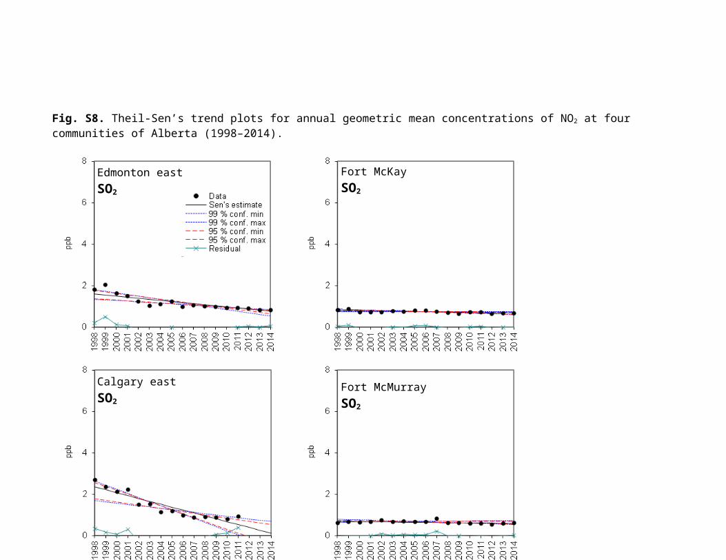
Fig. S9. Theil-Sen’s trend plots for annual geometric mean concentrations of SO2 at four communities of Alberta (1998–2014).
Edmonton east SO2
Calgary east SO2
Fort McKay SO2
Fort McMurray SO2
Fig. S10. Theil-Sen’s trend plots for annual geometric mean concentrations of PM2.5 at four communities of Alberta (1998–2014).
Edmonton central PM2.5
Edmonton east PM2.5
Calgary central PM2.5
Calgary east PM2.5
Fort McKay PM2.5
Fort McMurray PM2.5
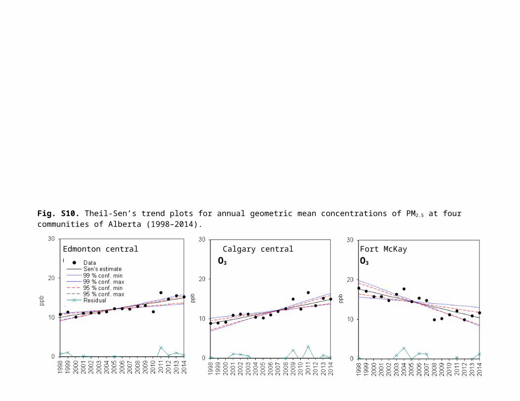
Fig. S11. Theil-Sen’s trend plots for annual geometric mean concentrations of O3 at four communities of Alberta (1998–2014).
Edmonton central O3
Edmonton east O3
Calgary central O3
Calgary east O3
Fort McKay O3
Fort McMurray O3
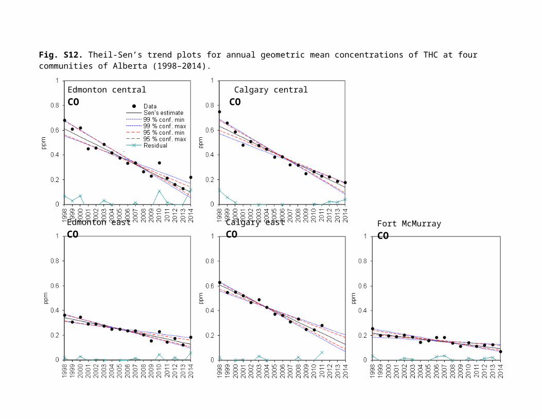
Fig. S12. Theil-Sen’s trend plots for annual geometric mean concentrations of THC at four communities of Alberta (1998–2014).
Edmonton central THC
Edmonton east THC
Calgary central THC
Calgary east THC
Fort McKay THC
Fort McMurray THC
Fig. S13. Theil-Sen’s trend plots for annual geometric mean concentrations of CO at four communities of Alberta (1998–2014).
Edmonton central CO
Edmonton east CO
Calgary central CO
Calgary east CO Fort McMurray CO
0 6 12 18 24
0
10
20
30
40
50
Time (h)
Con
cent
ratio
n (p
pb)
0 6 12 18 240
10
20
30
40
50
Time (h)
Con
cent
ratio
n (p
pb)
Fig. S14. Average diurnal (hourly) concentrations of NO2 and O3 at the major urban cities in Alberta for the period of 1998–2014 (missing data at 2:00 due to automatic instrument calibration).
Winter
Summer
1998–2014
1998–2014
NO2_Fort McMurray
NO2_Edmonton central
NO2_Calgary central
NO2_Fort McKayO3_Fort McKay
O3_Edmonton central
O3_Calgary central
O3_Fort McMurray
O3_Edmonton central
O3_Calgary central O3_Fort McKay
O3_Fort McMurray
NO2_Fort McMurray
NO2_Fort McKay
NO2_Edmonton central
NO2_Calgary central
0 6 12 18 240
10
20
30
Time (h)
PM
2.5
(µg/
m3)
0 6 12 18 240
10
20
30
Time (h)
PM
2.5
(µg/
m3)
PM2.5
PM2.5
Winter
Winter
Summer
SummerSO2 SO2
Calgary central
Edmonton centralFort McKay
Fort McMurrayFort McMurrayFort McKay
Edmonton centralCalgary central
1998–2014 1998–2014
Calgary east
Calgary eastEdmonton eastEdmonton east
Fort McKay
Fort McKay
Fort McMurrayFort McMurray
0 6 12 18 240
1
2
3
4
5
Time (h)
SO
2 (p
pb)
0 6 12 18 240
1
2
3
4
5
Time (h)
SO
2 (p
pb)
Fig. S15. Average diurnal (hourly) concentrations of PM2.5 and SO2 (missing data for SO2 at 2:00 due to automatic instrument calibration).
0 6 12 18 241.0
1.5
2.0
2.5
3.0
Time (h)
THC
(ppm
)
0 6 12 18 240
1
2
3
4
Time (h)
THC
(ppm
)
0 6 12 18 240.0
0.5
1.0
1.5
2.0
Time (h)
CO
(ppm
)
0 6 12 18 240.0
0.5
1.0
1.5
2.0
Time (h)
CO
(ppm
)
Winter 1998–2014 THC THC1998–2014 Summer
CO COWinter Summer
Edmonton central
Edmonton central
Calgary central
Calgary central
Fort McMurray
Fort McMurray
Edmonton centralCalgary central
Fort McMurray
Fort McKay
Fig. S16. Average diurnal (hourly) concentrations of THC and CO (missing data for SO2 at 2:00 due to automatic instrument calibration).
Fig. S17. Box plots of monthly NO2 concentrations over the period 1998–2014. Boxes represent 25th (lower quartile) and 75th (upper quartile)
percentile values, with median values as lines across the boxes, mean values as round black ball and minimum and maximum values as whiskers.
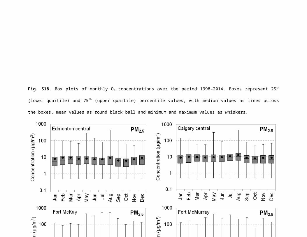
Fig. S18. Box plots of monthly O3 concentrations over the period 1998–2014. Boxes represent 25th (lower quartile) and 75th (upper quartile)
percentile values, with median values as lines across the boxes, mean values as round black ball and minimum and maximum values as whiskers.
Fig. S19. Box plots of monthly PM2.5 concentrations over the period 1998–2014. Boxes represent 25th (lower quartile) and 75th (upper quartile)
percentile values, with median values as lines across the boxes, mean values as round black ball and minimum and maximum values as whiskers.
Fig. S20. Box plots of monthly SO2 concentrations over the period 1998–2014. Boxes represent 25th (lower quartile) and 75th (upper quartile)
percentile values, with median values as lines across the boxes, mean values as round black ball and minimum and maximum values as whiskers.
Fig. S21. Box plots of monthly CO concentrations over the period 1998–2014. Boxes represent 25th (lower quartile) and 75th (upper quartile)
percentile values, with median values as lines across the boxes, mean values as round black ball and minimum and maximum values as whiskers.
1998
1999
2000
2001
2002
2003
2004
2005
2006
2007
2008
2009
2010
2011
2012
2013
2014
0
5
10
15
20
1 1
8
1
Number of 8 h O3 exceedances (> 65 ppb)Edmonton centralCalgary centralFort McKayFort McMurray
No
of O
3 ex
ceed
ance
s
1998
1999
2000
2001
2002
2003
2004
2005
2006
2007
2008
2009
2010
2011
2012
2013
2014
0
10
20
30
40
50
10
1 1
12
52
12
31 2
73
1 1 2 2 2
21
8
2
84
1 25
2 31 1
18
52
10
13 2
41 1 2
32
73
52
Number of 24 h PM2.5 exceedances (> 30 μg/m3)Edmonton centralCalgary centralFort McKayFort McMurray
No.
of P
M2.
5 ex
ceed
ance
s
a
b
Fig. S22. Total number of exceedances of Canada-Wide Standard for (a) 8 h O3 (65 ppb) and (b) 24 h PM2.5 (30 μg/m3) concentrations at the
community stations over the study period (1998–2014).
1-Ja
n-98
1-Ju
l-98
1-Ja
n-99
1-Ju
l-99
1-Ja
n-00
1-Ju
l-00
1-Ja
n-01
1-Ju
l-01
1-Ja
n-02
1-Ju
l-02
1-Ja
n-03
1-Ju
l-03
1-Ja
n-04
1-Ju
l-04
1-Ja
n-05
1-Ju
l-05
1-Ja
n-06
1-Ju
l-06
1-Ja
n-07
1-Ju
l-07
1-Ja
n-08
1-Ju
l-08
1-Ja
n-09
1-Ju
l-09
1-Ja
n-10
1-Ju
l-10
1-Ja
n-11
1-Ju
l-11
1-Ja
n-12
1-Ju
l-12
1-Ja
n-13
1-Ju
l-13
1-Ja
n-14
1-Ju
l-14
0
30
60
90
120
150
180
24 h PM2.5Edmonton central
μg/m
3
1-Ja
n-98
1-Ju
l-98
1-Ja
n-99
1-Ju
l-99
1-Ja
n-00
1-Ju
l-00
1-Ja
n-01
1-Ju
l-01
1-Ja
n-02
1-Ju
l-02
1-Ja
n-03
1-Ju
l-03
1-Ja
n-04
1-Ju
l-04
1-Ja
n-05
1-Ju
l-05
1-Ja
n-06
1-Ju
l-06
1-Ja
n-07
1-Ju
l-07
1-Ja
n-08
1-Ju
l-08
1-Ja
n-09
1-Ju
l-09
1-Ja
n-10
1-Ju
l-10
1-Ja
n-11
1-Ju
l-11
1-Ja
n-12
1-Ju
l-12
1-Ja
n-13
1-Ju
l-13
1-Ja
n-14
1-Ju
l-14
0
30
60
90
120
150
18024 h PM2.5Calgary central
μg/m
3
Fig. S23. PM2.5 concentrations (24 h) at Edmonton and Calgary central sites over the study period (1998–2014).
24 h Canada-Wide Standard
24 h Canada-Wide Standard
1-Ja
n-98
1-Ju
l-98
1-Ja
n-99
1-Ju
l-99
1-Ja
n-00
1-Ju
l-00
1-Ja
n-01
1-Ju
l-01
1-Ja
n-02
1-Ju
l-02
1-Ja
n-03
1-Ju
l-03
1-Ja
n-04
1-Ju
l-04
1-Ja
n-05
1-Ju
l-05
1-Ja
n-06
1-Ju
l-06
1-Ja
n-07
1-Ju
l-07
1-Ja
n-08
1-Ju
l-08
1-Ja
n-09
1-Ju
l-09
1-Ja
n-10
1-Ju
l-10
1-Ja
n-11
1-Ju
l-11
1-Ja
n-12
1-Ju
l-12
1-Ja
n-13
1-Ju
l-13
1-Ja
n-14
1-Ju
l-14
0
30
60
90
120
150
18024-h PM2.5Fort McKay
Fort McMurray
μg/m
3
Fig. S24. PM2.5 concentrations (24 h) in the AOSR over the study period (1998–2014).
24 h Canada-Wide Standard
1-Ja
n-11
11-J
an-1
121
-Jan
-11
31-J
an-1
110
-Feb
-11
20-F
eb-1
12-
Mar
-11
12-M
ar-1
122
-Mar
-11
1-A
pr-1
111
-Apr
-11
21-A
pr-1
11-
May
-11
11-M
ay-1
121
-May
-11
31-M
ay-1
110
-Jun
-11
20-J
un-1
130
-Jun
-11
10-J
ul-1
120
-Jul
-11
30-J
ul-1
19-
Aug
-11
19-A
ug-1
129
-Aug
-11
8-S
ep-1
118
-Sep
-11
28-S
ep-1
18-
Oct
-11
18-O
ct-1
128
-Oct
-11
7-N
ov-1
117
-Nov
-11
27-N
ov-1
17-
Dec
-11
17-D
ec-1
127
-Dec
-110
100
200
300
400
5001 h PM2.5Fort McKay
Fort McMurray
μg/m
3
Fig. S25. MODIS satellite image of wildfires on May 16, 2011 in Slave Lake, Alberta (a) and
impact on ambient PM2.5 concentrations in the AOSR (b).
May 16, 2011
Slave Lake
1 h AAAQO of 80 μg/m3
a
b
Fort McMurray
Fig. S26. Comparison of 1 h percentile concentrations between Canadian and major U.S. cities during 2012 using box-whisker plots; data for
Edmonton/Calgary are based on central stations except east stations for SO2.
0
10
20
30
40
50
60PM2.5Edmonton Downtown Calgary Downtown
Fort McKay Fort McMurrayToronto Downtown Montreal DowntownOttawa Downtown
98th
Per
cent
le P
M2.
5 (μ
g/m
3)
Fig. S27. Comparison of 98th percentile concentrations of PM2.5 between major Canadian cities over the period of 2003 to 2013
excluding year 2010 for Edmonton and 2011 for Fort McKay and Fort McMurray due to extreme wildfires impact.
24 h Canada-Wide Standard
Industrial emission trends
The National Pollutant Release Inventory (NPRI) reports annual releases of pollutants to air from
Canadian industrial facilities/operations (Environment Canada, 2015). Annual reported emissions of NOX,
SO2, and PM2.5 releases to air from industrial facilities/operations in Edmonton, Calgary and the
Athabasca Oil Sands Region (AOSR) were accessed from Environment Canada (2015) for the latest 12
years available (2003–2014) and are summarized in Table S3. NPRI quantities do not account for small
emission sources, such as small compressors and generators, and emissions from private/commercial
vehicles. Table S4 shows trends in NPRI reported industrial emissions for NOX, SO2, and PM2.5 using the
non-parametric (Mann-Kendall and Theil-Sen) approach.
Table S3. Reported NPRI emissions for NOX, SO2, and PM2.5 in Edmonton, Calgary and the Athabasca
Oil Sands Region (AOSR) for the period 2002–2014 (Environment Canada, 2015).
2014 71,234 84,702 3,290 4,250 9,035 168 29,039 45,762 3,9311Reported available NPRI emissions from oil sands and heavy oil facilities within 70-km around Fort McKay; –, not available.
Note: Methods used for quantifying annual releases of substances that are reported in NPRI can vary. Gases like NO x, and SO2 are based on continuous emission monitoring systems (CEMS), while PM2.5 is based on a combination of manual stack testing (Environment Canada, 2015). Environment Canada implements quality measures in an attempt to ensure that NPRI data maintains a high standard of accuracy, consistency and comprehensiveness. Facilities that meet NPRI reporting requirements are required to submit information that is true, accurate, and complete to the best of their knowledge and the Canadian Environmental Protection Act, 1999 sets out penalties for facilities that fail to report or that knowingly submit false or misleading information.
At Edmonton and Calgary, statistically significant downward trends for industrial emissions were
observed for NOX (p = 0.01) with annual decreases of –933 and –164 tonnes/year (–1.2% and –2.7% per
year), respectively over the 2003–2014 period. In contrast, in the AOSR a small upward trend was
Table S4. Reported NPRI emission trends for NOX, SO2, and PM2.5 in Edmonton, Calgary and the
Athabasca Oil Sands Region (AOSR) for the period 2002–2014.