Arsenic and Inorganic Arsenic Compounds - Tceq

Office of the Executive Director ___________________________________________________________

TEXAS COMMISSION ON ENVIRONMENTAL QUALITY

Development Support Document Final July 31, 2012 Accessible 2013

Arsenic and Inorganic Arsenic Compounds

CAS Registry Numbers:

7440-38-2 (Arsenic)

Prepared by

Neeraja K. Erraguntla, Ph.D.

Roberta L. Grant, Ph.D.

Toxicology Division

Arsenic and Inorganic Arsenic Compounds Page i

TABLE OF CONTENTS TABLE OF CONTENTS ............................................................................................................... I

LIST OF TABLES ....................................................................................................................... IV

LIST OF FIGURES ...................................................................................................................... V

ACRONYMS AND ABBREVIATIONS ................................................................................................. VI

CHAPTER 1 SUMMARY TABLES ...................................................................................................... 1

CHAPTER 2 MAJOR SOURCES AND USES, ATMOSPHERIC FATE, AMBIENT AIR CONCENTRATIONS, AND ROUTES OF EXPOSURE ........................................................................... 5

2.1 Natural Sources ..................................................................................................................... 5 2.2 Uses and Anthropogenic Sources ......................................................................................... 5 2.3 Atmospheric Fate of Arsenic ................................................................................................ 6 2.4 Ambient Levels of Arsenic in Air and Routes of Exposure ................................................. 6

CHAPTER 3 ACUTE EVALUATION .................................................................................................. 7

3.1 Health-Based Acute ReV and ESL ....................................................................................... 7 3.1.1 Physical/Chemical Properties........................................................................................ 7 3.1.2 Key Studies ..................................................................................................................... 8

3.1.2.1 Rationale for the Evaluation of Arsenic Trioxide (ATO) ....................................... 8 3.1.2.2 Human Studies ........................................................................................................ 8

3.1.2.2.1 Respiratory and Gastrointestinal Effects ......................................................... 8 3.1.2.2.2 Developmental and Reproductive Studies ....................................................... 8

3.1.2.2.2.1 Nordstrom et al. (1978, 1979a, 1979b) ..................................................... 9 3.1.2.2.2.2 Ihrig et al. (1998) ...................................................................................... 9

3.1.2.3 Animal Studies ........................................................................................................ 9 3.1.2.3.1 Developmental and Reproductive Studies ....................................................... 9 3.1.2.3.2 Holson et al. (1999) - Key study .................................................................... 10

3.1.2.3.2.1 Preliminary Exposure Range-Finding Studies ........................................ 10 3.1.2.3.2.2 Maternal Effects from the Second Preliminary Study ............................ 10 3.1.2.3.2.3 Fetal Toxicity from the Second Preliminary Study ................................ 11 3.1.2.3.2.4 Definitive Study ...................................................................................... 11 3.1.2.3.2.5 Summary of the Definitive Study ........................................................... 13

3.1.2.3.3 Nagymajtenyi et al. (1985) - Supporting Study .............................................. 13 3.1.2.3.4 Immunotoxicity Study (Supporting Study) (Burchiel et al. 2009) .................. 15

3.1.3 Mode-of-Action (MOA) Analysis ................................................................................. 16 3.1.3.1 Toxicokinetic Summary ........................................................................................ 16 3.1.3.2 Interaction with Sulfhydryl-Containing Enzymes ................................................ 17 3.1.3.3 Metabolism ........................................................................................................... 17 3.1.3.4 Oxidative Stress .................................................................................................... 19

3.1.4 Dose Metric .................................................................................................................. 19 3.1.5 Point of Departure (POD) for the Key Study ............................................................... 19

Arsenic and Inorganic Arsenic Compounds Page ii

3.1.6 Dosimetric Adjustments ............................................................................................... 19 3.1.6.1 Default Exposure Duration Adjustments .............................................................. 19 3.1.6.2 Default Dosimetry Adjustments from Animal-to-Human Exposure .................... 20 3.1.6.3 Critical Effect and Adjustments to the PODHEC ................................................... 21

3.1.7 Adjustments of the PODHEC ......................................................................................... 21 3.1.8 Health-Based Acute ReV for ATO ................................................................................ 21 3.1.9 Health-Based Acute ReV and acuteESL for Arsenic....................................................... 21 3.1.10 Comparison of Results ............................................................................................... 23

3.2 Welfare-Based acuteESLs ..................................................................................................... 23 3.2.1 Odor Perception ........................................................................................................... 23 3.2.2 Vegetation Effects ........................................................................................................ 23

3.3 Short-Term ESL and Values for Air Monitoring Evaluation ............................................. 23

CHAPTER 4 CHRONIC EVALUATION ............................................................................................ 24

4.1 Noncarcinogenic Potential .................................................................................................. 24 4.1.1 Physical/Chemical Properties...................................................................................... 24 4.1.2 Key Human Studies ...................................................................................................... 24

4.1.2.1 Vascular and Cardiovascular Effects .................................................................... 24 4.1.2.1 Blom et al. (1985) ............................................................................................. 25 4.1.2.1.2 Lagerkvist and Zetterlund (1994) .................................................................. 26 4.1.2.1.3 Lagerkvist et al. (1986) .................................................................................. 27

4.1.2.2 Respiratory, Ocular, Dermal, and Gastrointestinal Effects ................................... 28 4.1.2.2.1 Perry et al. (1948) .......................................................................................... 28 4.1.2.2.2 Lubin et al. (2000) ......................................................................................... 29

4.1.2.3 Neurological Effects ............................................................................................. 29 4.1.2.3.1 Feldman et al. (1979) ..................................................................................... 30 4.1.2.3.2 Buchancova et al. (1998) ............................................................................... 30

4.1.3 MOA Analysis .............................................................................................................. 30 4.1.4 Dose Metric .................................................................................................................. 30 4.1.5 PODs for Key Studies .................................................................................................. 30 4.1.6 Health-Based Chronic ReV for ATO ............................................................................ 30

4.2 Carcinogenic Potential ........................................................................................................ 31 4.2.1 Weight of Evidence (WOE) Evaluation ........................................................................ 31

4.2.1.1 WOE from Epidemiological Studies Included in ATSDR (2007)........................ 31 4.2.1.1.1 Overview ........................................................................................................ 31 4.2.1.1.2 ASARCO Copper Smelter in Tacoma, Washington ....................................... 32 4.2.1.1.3 Anaconda Copper Smelter in Montana ......................................................... 32 4.2.1.1.4 Eight US Copper Smelters ............................................................................. 33 4.2.1.1.5 Ronnskar Copper Smelter in Sweden ............................................................. 33 4.2.1.1.6 Other Types of Nonrespiratory Cancer ......................................................... 34

4.2.1.2 WOE from Other Epidemiological Studies .......................................................... 35 4.2.1.2.1 United Kingdom (UK) Tin Smelter Study ...................................................... 35 4.2.1.2.2 China Mine Study ........................................................................................... 35

4.2.1.3 WOE from Animal Studies ................................................................................... 37

Arsenic and Inorganic Arsenic Compounds Page iii

4.2.1.4 WOE Classifications ............................................................................................. 37 4.2.2 Carcinogenic MOA ...................................................................................................... 37

4.2.2.1 Oxidative Stress .................................................................................................... 39 4.2.2.2 Altered Growth Factors→Cell Proliferation→Promotion of Carcinogenesis ...... 39 4.2.2.3 Genotoxicity .......................................................................................................... 39 4.2.2.4 Additional Mechanisms of Toxicity ..................................................................... 40

4.2.3 Dose Metric, Relevant Cancer Endpoint, and Dose-Response Assessment ................ 40 4.2.3.1 Dose Metric ........................................................................................................... 40 4.2.3.2 Dose Response Assessment .................................................................................. 41

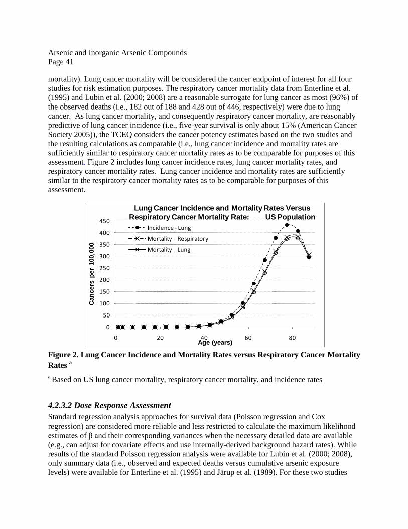
4.2.4 Epidemiological Studies used to Develop URFs ......................................................... 42 4.2.4.1 Enterline et al. (1982, 1987a, 1987b, and 1995) ................................................... 44

4.2.4.1.1 Slope Parameter (β) Estimates ...................................................................... 46 4.2.4.1.1.1 Enterline et al. (1995) Dose-Response .................................................... 46 4.2.4.1.1.2 Viren and Silvers (1999) Dose-Response ............................................... 47 4.2.4.1.1.3 Adjusting for Year of Hire as a Nonparametric Function ....................... 48

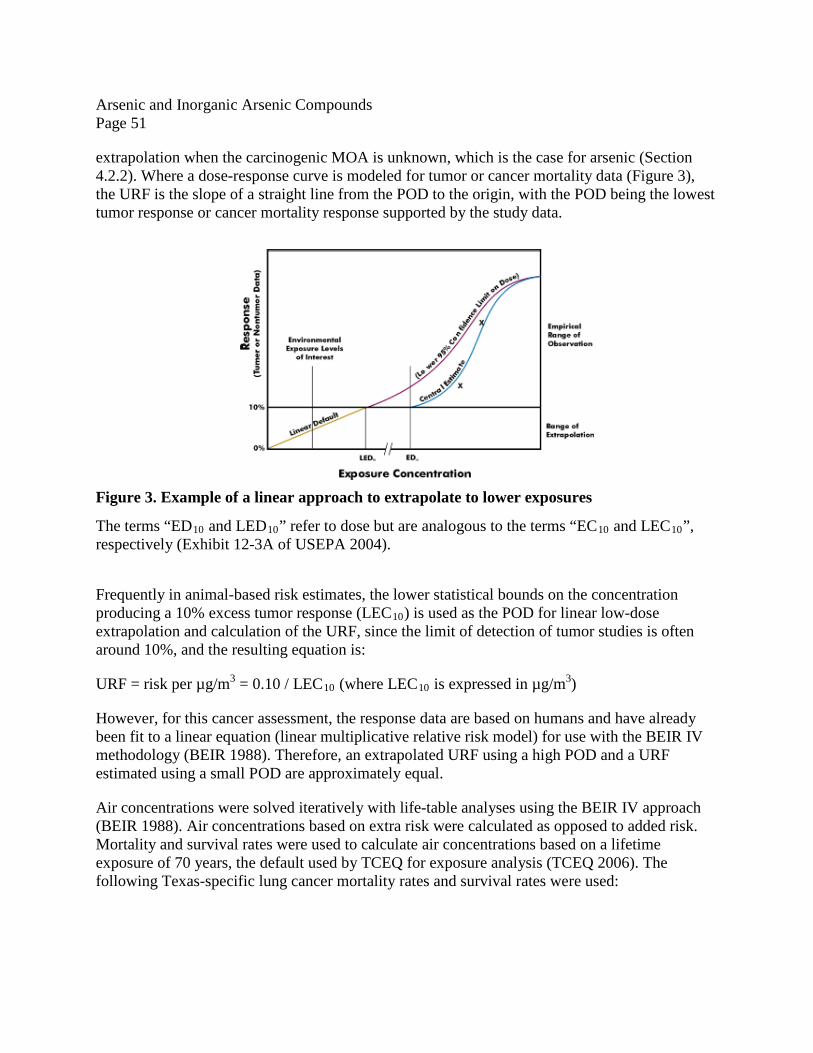
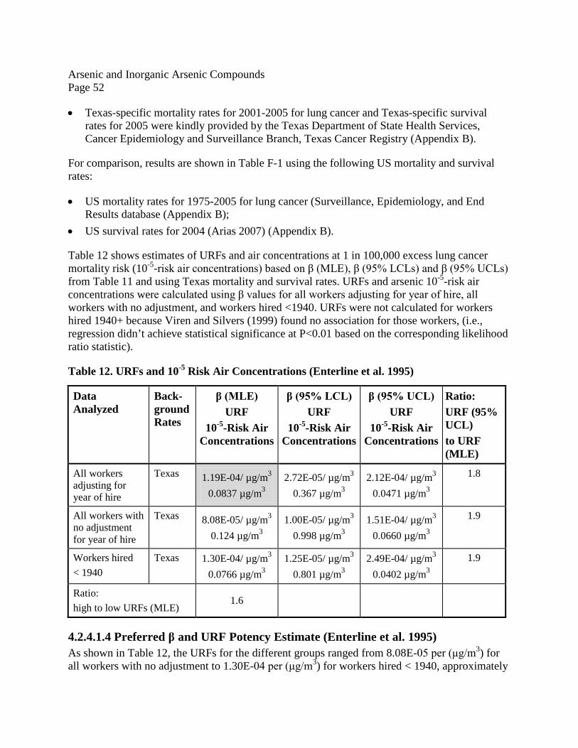
4.2.4.1.2 Dosimetric Adjustments ................................................................................. 50 4.2.4.1.3 Unit Risk Factors (URFs) and Air Concentrations at 1 in 100,000 Excess Lung Cancer Mortality ................................................................................................. 50 4.2.4.1.4 Preferred β and URF Potency Estimate (Enterline et al. 1995) .................... 52

4.2.4.2 Lubin et al. (2000, 2008)....................................................................................... 53 4.2.4.2.1 Slope Parameter (β) Estimates ...................................................................... 54

4.2.4.2.1.1 Lubin et al. (2000) ................................................................................... 54 4.2.4.2.1.2 Lubin et al. (2008) ................................................................................... 55

4.2.4.2.1.2.1 Concentration as an Effect-Modification Factor.............................. 55 4.2.4.2.1.2.2 Models in Lubin et al. (2008) .......................................................... 55 4.2.4.2.1.2.3 Nonparametric Effects of Time since Last Exposure and Age ........ 56 4.2.4.2.1.2.4 Maximum Likelihood Estimates of the Slope with the Linear-Exponential Model ................................................................................................ 57 4.2.4.2.1.2.5 Maximum Likelihood Estimates of the Slope with the Linear Multiplicative Model ............................................................................................ 58

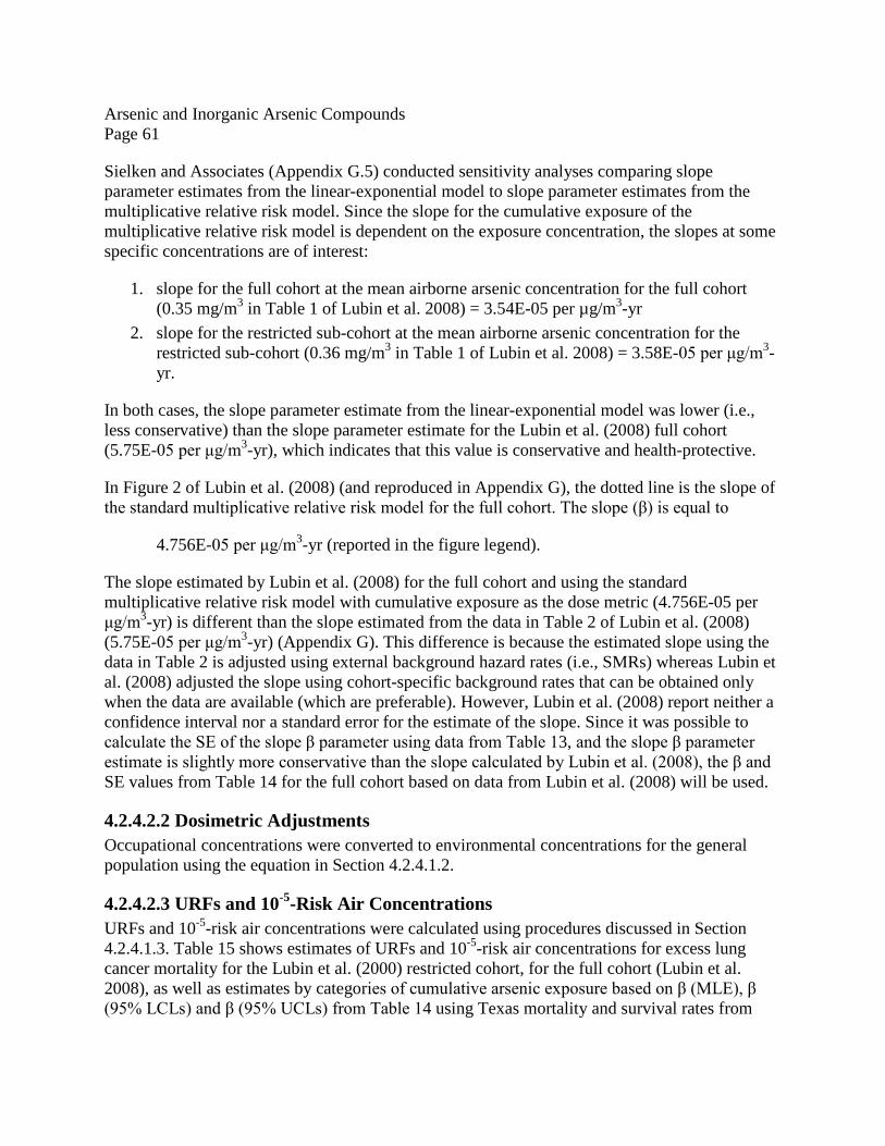
4.2.4.2.2 Dosimetric Adjustments ................................................................................. 61 4.2.4.2.3 URFs and 10-5-Risk Air Concentrations ........................................................ 61 4.2.4.2.4 Preferred β and URF Potency Estimate (Lubin et al. 2000, 2008) ............... 62

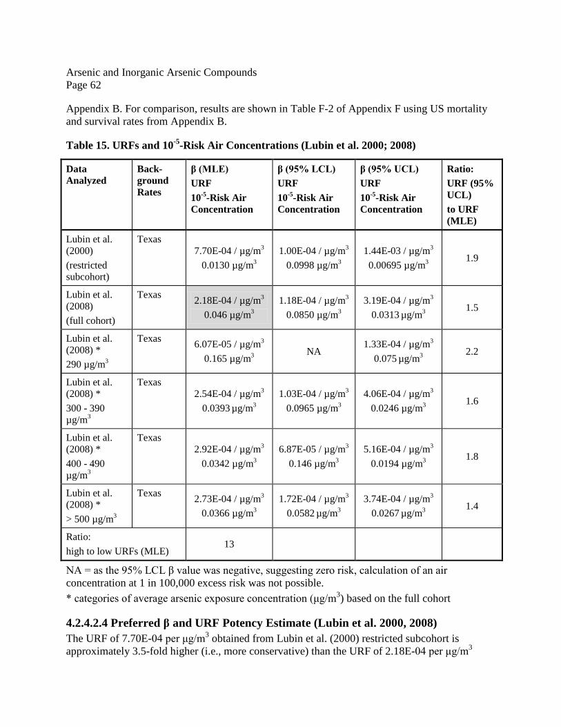
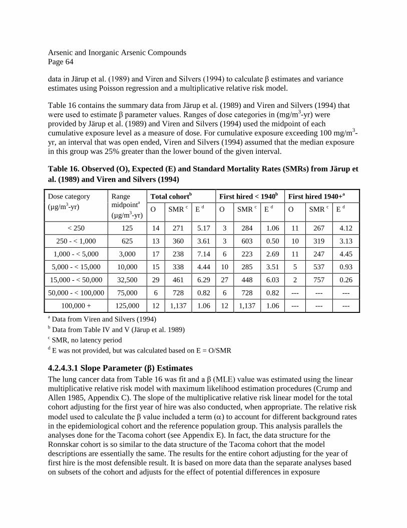
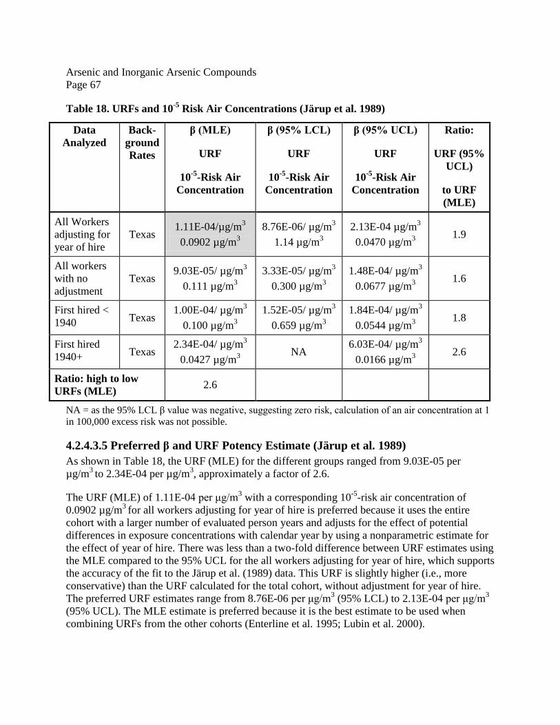
4.2.4.3 Järup et al. (1989); Viren and Silvers (1994) ........................................................ 63 4.2.4.3.1 Slope Parameter (β) Estimates ...................................................................... 64 4.2.4.3.2 Sensitivity Analyses ........................................................................................ 65 4.2.4.3.3 Dosimetric Adjustments ................................................................................. 66 4.2.4.3.4 URFs and 10-5-Risk Air Concentrations ........................................................ 66 4.2.4.3.5 Preferred β and URF Potency Estimate (Järup et al. 1989) ......................... 67

4.2.4.4 Jones et al. (2007) ................................................................................................. 68 4.2.4.5 Combined – Analysis Using Inverse Variance of the URFs to weigh Individual URFs ................................................................................................................................. 69 4.2.4.6 Sensitivity Analysis with Various Meta-Analysis Procedures ............................. 72

Arsenic and Inorganic Arsenic Compounds Page iv

4.2.4.6.1 Meta-Analysis Using Inverse Variance of the Estimated Slopes to Weight Individual Slopes ........................................................................................................... 72 4.2.4.6.2 Meta-Analyses Using Dose-Response Models to Fit the Combined Data ..... 73

4.2.5 Final URF and chronicESLlinear(c) .................................................................................... 79 4.2.6 Evaluating Susceptibility from Early-Life Exposures .................................................. 79 4.2.7 Uncertainty Analysis .................................................................................................... 79

4.2.7.1 Dose-Response Modeling ..................................................................................... 79 4.2.7.2 Epidemiological Occupational Studies ................................................................. 80

4.2.7.2.1 Estimating Risks for other Potentially Sensitive Subpopulations .................. 80 4.2.7.2.2 Estimating Risks for the General Population from Occupational Workers .. 81 4.2.7.2.3 Occupational Exposure Estimation Error ..................................................... 81 4.2.7.2.4 Uncertainty Due to Co-Exposures to other Compounds ............................... 82 4.2.7.2.5 Uncertainty Due to Other Reasons ................................................................ 83

4.2.8 Comparison of TCEQ and USEPA’s URF ................................................................... 83 4.3 Welfare-Based Chronic ESL .............................................................................................. 84 4.4 Long-Term ESL and Values for Air Monitoring Evaluation ............................................. 84

CHAPTER 5 REFERENCES ............................................................................................................. 85

5.1 References Cited in DSD .................................................................................................... 85 5.2 Other References Reviewed by TCEQ ............................................................................... 94

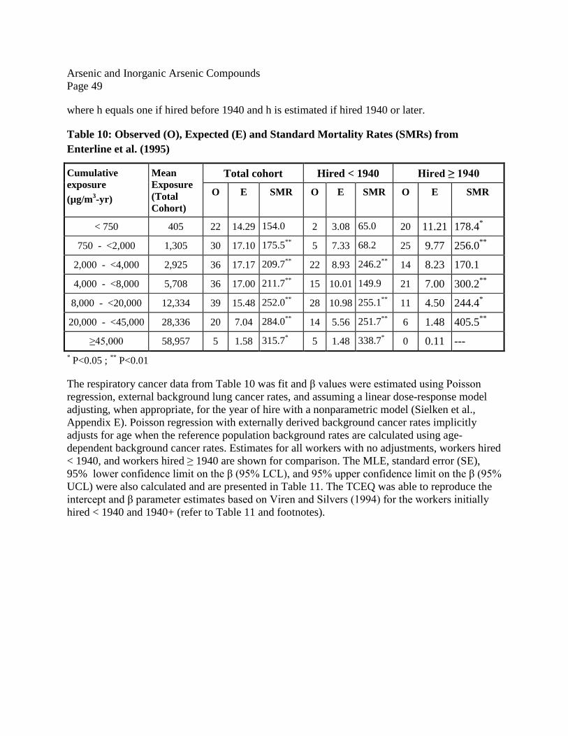
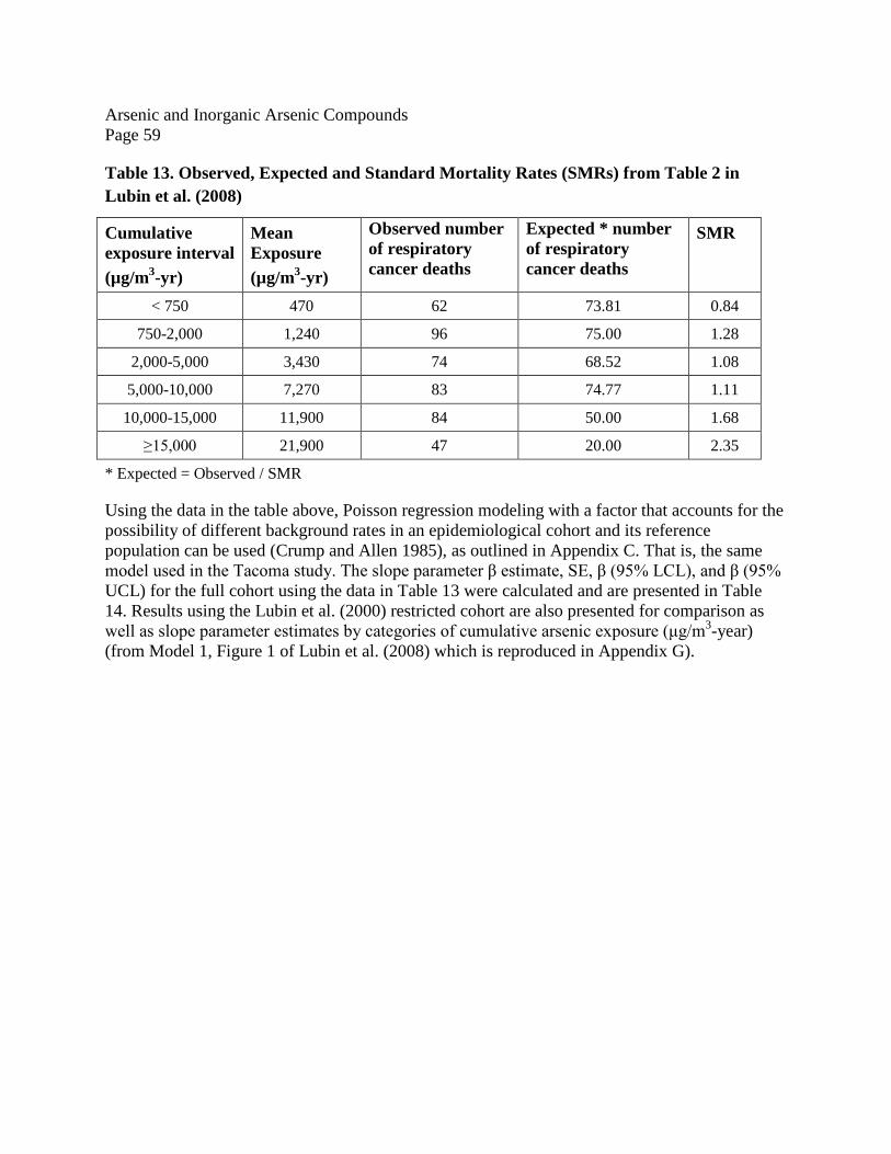
LIST OF TABLES Table 1. Air Monitoring Comparison Values (AMCVs) for Ambient Air for Arsenic (As) - Particle size < 10 µm ...................................................................................................................... 1 Table 2. Air Permitting Effects Screening Levels (ESLs) for Arsenic (As) - Particle size < 10 µm......................................................................................................................................................... 2 Table 3. Physical and Chemical Properties of Arsenic and Inorganic Arsenic Compounds .......... 3 Table 4. Physical and Chemical Properties of Arsenic and Inorganic Arsenic Compounds (continued) ...................................................................................................................................... 4 Table 5. Survival, Pregnancy Status, Food Consumption, and Body Weight Data during Gestation for Rats Exposed by Inhalation to Arsenic Trioxide (ATO) Holson et al. 1999 .......... 12 Table 6. Mice Fetal Developmental Effects Following Maternal Exposure to Inhaled Arsenic 1 14 Table 7. Summary Information and Comparison of the Acute Inhalation Studies ....................... 16 Table 8. Derivation of the Acute ReV and acuteESL for ATO and Arsenic ................................ 22 Table 9. Epidemiological Studies with Adequate Dose-Response Data ...................................... 44 Table 10: Observed (O), Expected (E) and Standard Mortality Rates (SMRs) from Enterline et al. (1995) ............................................................................................................................................ 49 Table 11. Beta (β), Standard Error (SE), and 95% Lower Confidence Limit (LCL) and Upper Confidence Limit (UCL) β Values (Enterline et al. 1995) a ......................................................... 50 Table 12. URFs and 10-5 Risk Air Concentrations (Enterline et al. 1995) ................................... 52 Table 13. Observed, Expected and Standard Mortality Rates (SMRs) from Table 2 in Lubin et al. (2008) ............................................................................................................................................ 59

Arsenic and Inorganic Arsenic Compounds Page v

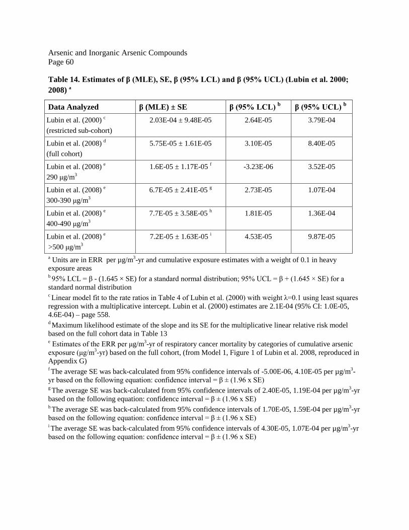
Table 14. Estimates of β (MLE), SE, β (95% LCL) and β (95% UCL) (Lubin et al. 2000; 2008) a....................................................................................................................................................... 60 Table 15. URFs and 10-5-Risk Air Concentrations (Lubin et al. 2000; 2008) .............................. 62 Table 16. Observed (O), Expected (E) and Standard Mortality Rates (SMRs) from Järup et al. (1989) and Viren and Silvers (1994) ............................................................................................ 64 Table 17. Estimates of β (MLE), SE, β (95% LCL) and β (95% UCL) (Järup et al. 1989)a ........ 65 Table 18. URFs and 10-5 Risk Air Concentrations (Järup et al. 1989) ......................................... 67 Table 19. Preferred URFs and 10-5-Risk Air Concentrations from the Tacoma, Montana and Swedish Cohort (Texas Background Rates) ................................................................................. 69 Table 20. Estimates of the intercept, slope, standard error and 95% UCL on the slopes resulting from meta-analyses that combine the Tacoma, Montana and Sweden cohorts ............................ 74 Table 21. Estimated URF and 95% UCL on the URF resulting from meta-analyses that combine the Tacoma, Montana and Sweden cohorts .................................................................................. 78

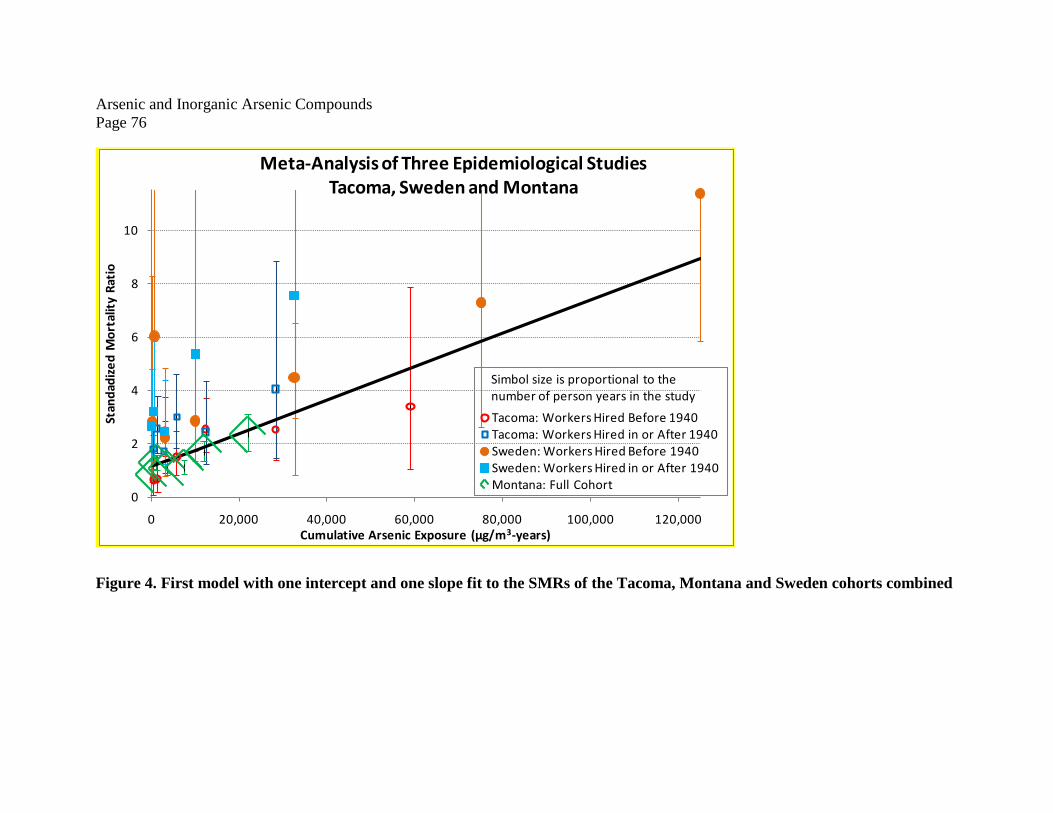
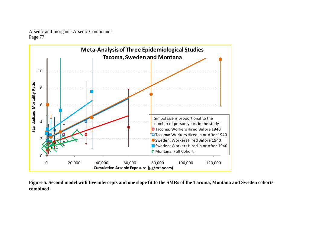
LIST OF FIGURES Figure 1. Inorganic arsenic biotransformation pathway. SAM, S-adenosylmethionine, SAHC, S-adenosylhomocysteine (Source: Aposhian et al. 2000 as cited in ATSDR 2007) ........................ 18 Figure 2. Lung Cancer Incidence and Mortality Rates versus Respiratory Cancer Mortality Rates a ........................................................................................................................................... 41 Figure 3. Example of a linear approach to extrapolate to lower exposures .................................. 51 Figure 4. First model with one intercept and one slope fit to the SMRs of the Tacoma, Montana and Sweden cohorts combined...................................................................................................... 76 Figure 5. Second model with five intercepts and one slope fit to the SMRs of the Tacoma, Montana and Sweden cohorts combined ...................................................................................... 77

Arsenic and Inorganic Arsenic Compounds Page vi

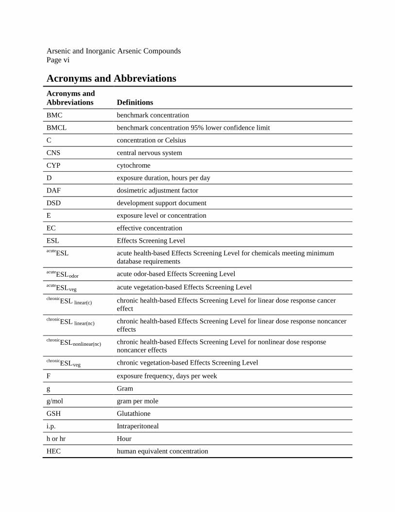
Acronyms and Abbreviations Acronyms and Abbreviations Definitions BMC benchmark concentration

BMCL benchmark concentration 95% lower confidence limit

C concentration or Celsius

CNS central nervous system

CYP cytochrome

D exposure duration, hours per day

DAF dosimetric adjustment factor

DSD development support document

E exposure level or concentration

EC effective concentration

ESL Effects Screening Level acuteESL acute health-based Effects Screening Level for chemicals meeting minimum

database requirements acuteESLodor acute odor-based Effects Screening Level acuteESLveg

acute vegetation-based Effects Screening Level chronicESL linear(c)

chronic health-based Effects Screening Level for linear dose response cancer effect

chronicESL linear(nc) chronic health-based Effects Screening Level for linear dose response noncancer

effects chronicESLnonlinear(nc)

chronic health-based Effects Screening Level for nonlinear dose response noncancer effects

chronicESLveg chronic vegetation-based Effects Screening Level

F exposure frequency, days per week

g Gram

g/mol gram per mole

GSH Glutathione

i.p. Intraperitoneal

h or hr Hour

HEC human equivalent concentration

Arsenic and Inorganic Arsenic Compounds Page vii

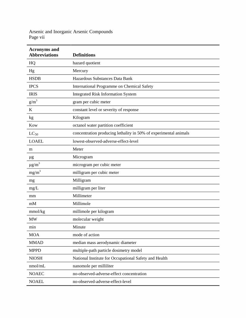
Acronyms and Abbreviations Definitions HQ hazard quotient

Hg Mercury

HSDB Hazardous Substances Data Bank

IPCS International Programme on Chemical Safety

IRIS Integrated Risk Information System

g/m3 gram per cubic meter

K constant level or severity of response

kg Kilogram

Kow octanol water partition coefficient

LC50 concentration producing lethality in 50% of experimental animals

LOAEL lowest-observed-adverse-effect-level

m Meter

µg Microgram

µg/m3 microgram per cubic meter

mg/m3 milligram per cubic meter

mg Milligram

mg/L milligram per liter

mm Millimeter

mM Millimole

mmol/kg millimole per kilogram

MW molecular weight

min Minute

MOA mode of action

MMAD median mass aerodynamic diameter

MPPD multiple-path particle dosimetry model

NIOSH National Institute for Occupational Safety and Health

nmol/mL nanomole per milliliter

NOAEC no-observed-adverse-effect concentration

NOAEL no-observed-adverse-effect-level

Arsenic and Inorganic Arsenic Compounds Page viii

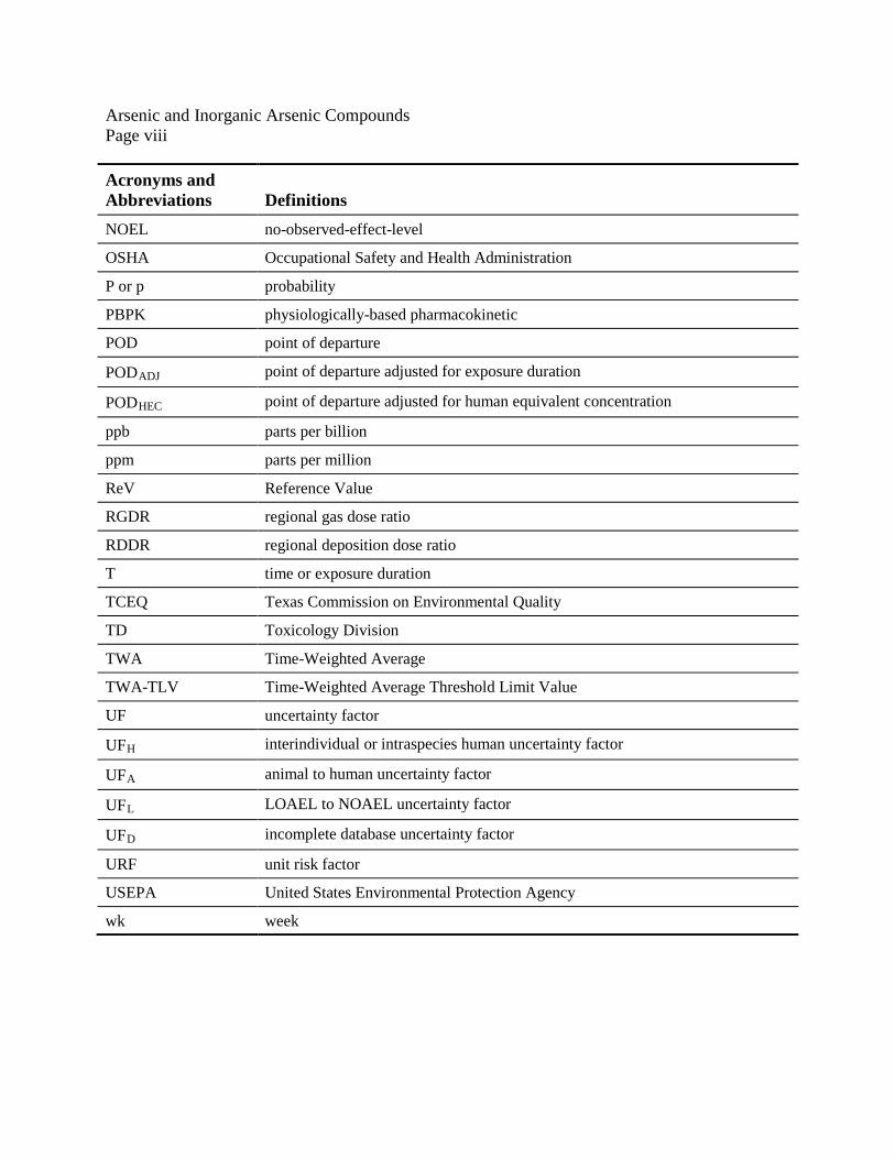
Acronyms and Abbreviations Definitions NOEL no-observed-effect-level

OSHA Occupational Safety and Health Administration

P or p probability

PBPK physiologically-based pharmacokinetic

POD point of departure

PODADJ point of departure adjusted for exposure duration

PODHEC point of departure adjusted for human equivalent concentration

ppb parts per billion

ppm parts per million

ReV Reference Value

RGDR regional gas dose ratio

RDDR regional deposition dose ratio

T time or exposure duration

TCEQ Texas Commission on Environmental Quality

TD Toxicology Division

TWA Time-Weighted Average

TWA-TLV Time-Weighted Average Threshold Limit Value

UF uncertainty factor

UFH interindividual or intraspecies human uncertainty factor

UFA animal to human uncertainty factor

UFL LOAEL to NOAEL uncertainty factor

UFD incomplete database uncertainty factor

URF unit risk factor

USEPA United States Environmental Protection Agency

wk week

Arsenic and Inorganic Arsenic Compounds Page 1

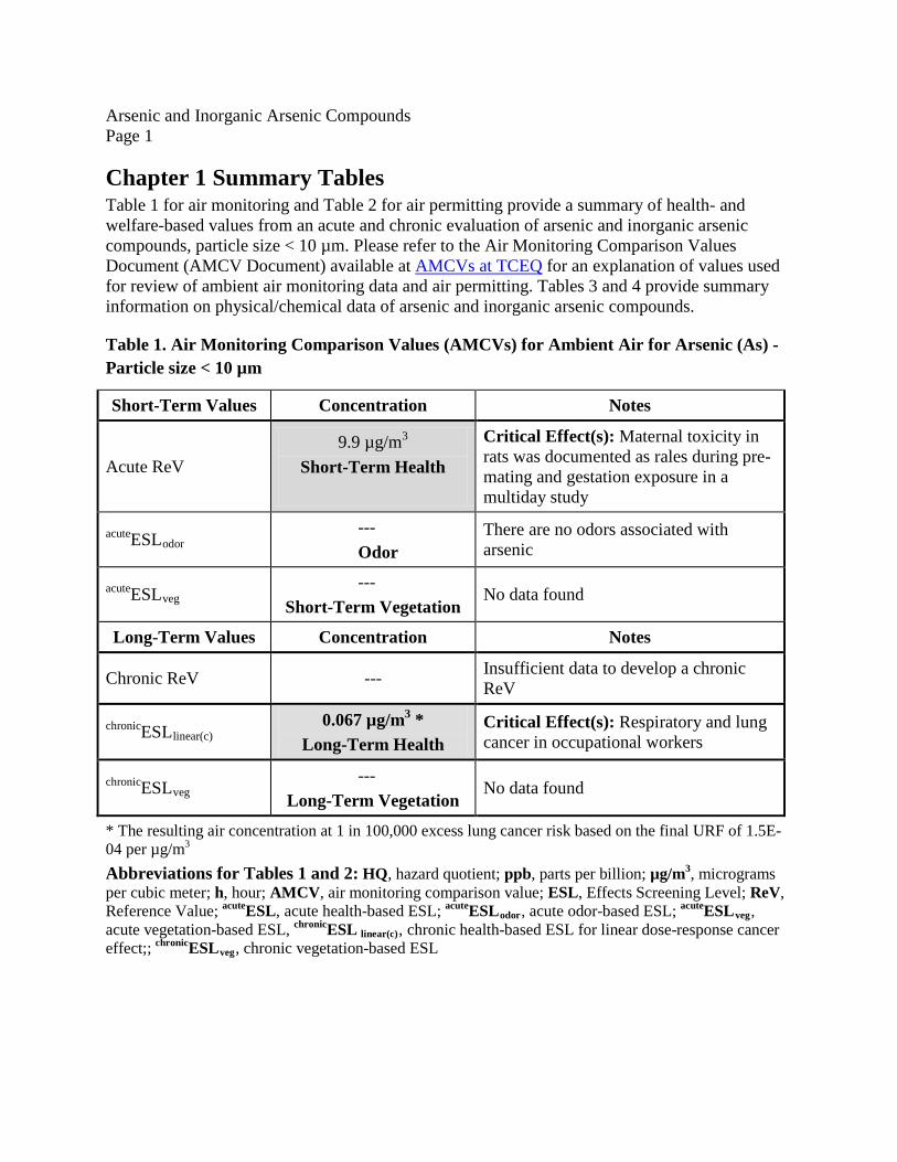
Chapter 1 Summary Tables Table 1 for air monitoring and Table 2 for air permitting provide a summary of health- and welfare-based values from an acute and chronic evaluation of arsenic and inorganic arsenic compounds, particle size < 10 µm. Please refer to the Air Monitoring Comparison Values Document (AMCV Document) available at AMCVs at TCEQ for an explanation of values used for review of ambient air monitoring data and air permitting. Tables 3 and 4 provide summary information on physical/chemical data of arsenic and inorganic arsenic compounds.

Table 1. Air Monitoring Comparison Values (AMCVs) for Ambient Air for Arsenic (As) - Particle size < 10 µm

Short-Term Values Concentration Notes

Acute ReV 9.9 µg/m3

Short-Term Health

Critical Effect(s): Maternal toxicity in rats was documented as rales during pre-mating and gestation exposure in a multiday study

acuteESLodor --- Odor

There are no odors associated with arsenic

acuteESLveg ---

Short-Term Vegetation No data found

Long-Term Values Concentration Notes

Chronic ReV --- Insufficient data to develop a chronic ReV

chronicESLlinear(c) 0.067 µg/m3 *

Long-Term Health Critical Effect(s): Respiratory and lung cancer in occupational workers

chronicESLveg ---

Long-Term Vegetation No data found

* The resulting air concentration at 1 in 100,000 excess lung cancer risk based on the final URF of 1.5E-04 per µg/m3 Abbreviations for Tables 1 and 2: HQ, hazard quotient; ppb, parts per billion; µg/m3, micrograms per cubic meter; h, hour; AMCV, air monitoring comparison value; ESL, Effects Screening Level; ReV, Reference Value; acuteESL, acute health-based ESL; acuteESLodor, acute odor-based ESL; acuteESLveg, acute vegetation-based ESL, chronicESL linear(c), chronic health-based ESL for linear dose-response cancer effect;; chronicESLveg, chronic vegetation-based ESL

http://www.tceq.state.tx.us/implementation/tox/AirToxics.html


Table 2. Air Permitting Effects Screening Levels (ESLs) for Arsenic (As) - Particle size < 10 µm

Short-Term Values Concentration Notes

acuteESL (HQ = 0.3)

3 µg/m3 a Short-Term ESL for Air Permit Reviews

Critical Effect(s): Maternal toxicity in rats was documented as rales during pre-mating and gestation exposure in a multiday study

acuteESLodor --- There are no odors associated with arsenic

acuteESLveg --- No data found

Long-Term Values Concentration Notes chronicESLnonlinear(nc)

(HQ = 0.3) --- Insufficient data to develop a

chronic ReV

chronicESLlinear(c)

0.067 µg/m3 b Long-Term ESL for Air Permit Reviews

Critical Effect(s): Respiratory and lung cancer in occupational workers

chronicESLveg --- No data found

a Based on the acute ReV of 9.9 µg/m3 multiplied by 0.3 (i.e., HQ = 0.3) to account for cumulative and aggregate risk during the air permit review. b The resulting air concentration at a 1 in 100,000 excess lung cancer risk based on the final URF of 1.5E-04 per µg/m3


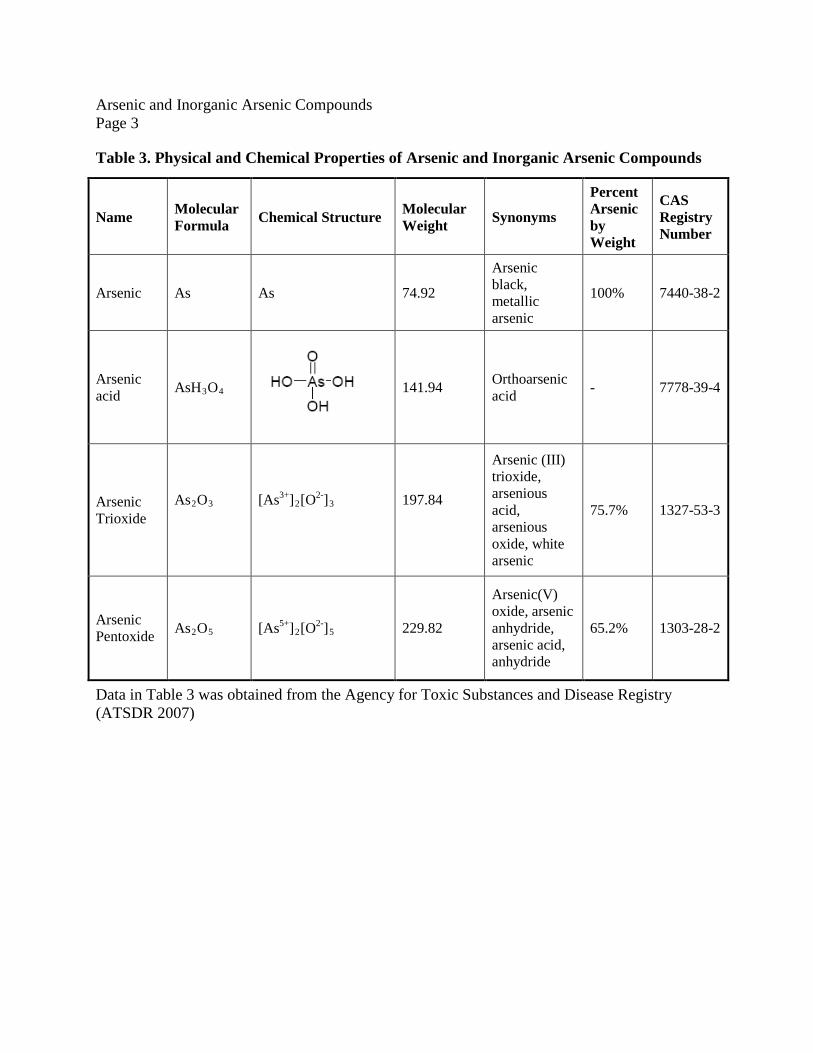
Table 3. Physical and Chemical Properties of Arsenic and Inorganic Arsenic Compounds

Name Molecular Formula Chemical Structure Molecular

Weight Synonyms

Percent Arsenic by Weight

CAS Registry Number

Arsenic As As 74.92

Arsenic black, metallic arsenic

100% 7440-38-2

Arsenic acid AsH3O4

141.94 Orthoarsenic acid - 7778-39-4

Arsenic Trioxide

As2O3

[As3+]2[O2-]3

197.84

Arsenic (III) trioxide, arsenious acid, arsenious oxide, white arsenic

75.7% 1327-53-3

Arsenic Pentoxide As2O5 [As5+]2[O2-]5 229.82

Arsenic(V) oxide, arsenic anhydride, arsenic acid, anhydride

65.2% 1303-28-2

Data in Table 3 was obtained from the Agency for Toxic Substances and Disease Registry (ATSDR 2007)


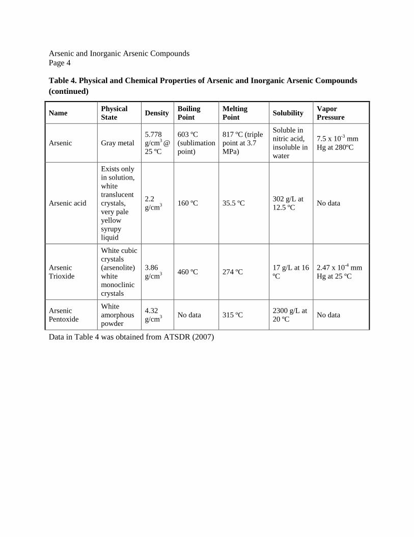
Table 4. Physical and Chemical Properties of Arsenic and Inorganic Arsenic Compounds (continued)

Name Physical State Density Boiling

Point Melting Point Solubility Vapor

Pressure

Arsenic Gray metal 5.778 g/cm3 @ 25 ºC

603 ºC (sublimation point)

817 ºC (triple point at 3.7 MPa)

Soluble in nitric acid, insoluble in water

7.5 x 10-3 mm Hg at 280ºC

Arsenic acid

Exists only in solution, white translucent crystals, very pale yellow syrupy liquid

2.2 g/cm3 160 ºC 35.5 ºC 302 g/L at

12.5 ºC No data

Arsenic Trioxide

White cubic crystals (arsenolite) white monoclinic crystals

3.86 g/cm3 460 ºC 274 ºC 17 g/L at 16

ºC 2.47 x 10-4 mm Hg at 25 ºC

Arsenic Pentoxide

White amorphous powder

4.32 g/cm3 No data 315 ºC 2300 g/L at

20 ºC No data

Data in Table 4 was obtained from ATSDR (2007)


Chapter 2 Major Sources and Uses, Atmospheric Fate, Ambient Air Concentrations, and Routes of Exposure

2.1 Natural Sources Arsenic is widely distributed in the earth’s crust, which contains approximately 3.4 parts per million (ppm) arsenic (ATSDR 2007). In nature, a small proportion of arsenic exists in its elemental form. It is, however, present predominantly in minerals. According to the United States Geological Survey (USGS), the most widespread natural source of arsenic is pyrite, a common mineral composed of iron, sulfur, and arsenic. Arsenic is released naturally into the environment during the weathering of rocks as windblown dust, volcanic eruptions, forest fires, and volatilization of methylarsines from the soil (ATSDR 2007).

2.2 Uses and Anthropogenic Sources While natural sources contribute to a small extent, the majority of arsenic released into the environment is from anthropogenic sources. Arsenic found in mineral ores is released as a byproduct into the environment during the mining and smelting of copper, lead, cobalt, and gold ores. The USGS reported the average arsenic concentration for United States (US) coal to be about 24 ppm. In addition to nonferrous metal mining and smelting operations, arsenic is also released into the environment during pesticide applications, coal combustion, wood combustion, and waste incineration processes. Chromated copper arsenate (CCA) is a chemical wood preservative containing chromium, copper and arsenic. Since the 1940s, CCA has been widely used in outdoor residential settings, such as decks and playsets to protect wood from rotting due to insects and microbial agents. The USEPA classified CCA as a restricted-use product, for use only by certified pesticide applicators, and in the US pressure treated wood containing CCA is no longer being produced for use in most residential settings, including decks and play sets.

Arsenic in the form of gallium arsenide (GaAs) is a major component in semi-conductors for telecommunications, solar cells, and space research. Arsenic is an important alloying element in ammunition and as an anti-friction additive to metals used for bearings. It is also used to strengthen lead acid storage battery grids (ATSDR 2007). Further, arsenic trioxide (ATO) and arsenic acid have long been used as decolorizers and are important components in the production and manufacture of glassware.

Historically arsenic has also played a major role as a medicinal agent and various compounds of arsenic have been used in homeopathic and veterinary medicine to treat various disorders of the skin and respiratory system both in the US and in other countries. Some examples of arsenic use have been to treat psoriasis and syphilis. Interestingly, ATO has been re-introduced as a potential drug to treat acute promyelocytic leukemia (ATSDR 2007).

In the US, the use of inorganic arsenicals has decreased to a large extent due to the ban on production. However, organic arsenicals are still present in the US as herbicides and as antimicrobial additives for animal and poultry feed (ATSDR 2007), and all of the arsenic used presently is imported from other countries.


2.3 Atmospheric Fate of Arsenic Arsenic is an element and therefore cannot be destroyed in the environment. It can only change its form or become attached or get separated from particles. While arsenic can exist in both organic and inorganic forms, and in vapor and particulate states, the predominant form in the atmospheric air is inorganic arsenic in the particulate state. Arsenic in vapor form is present to a minor extent and has been measured in and around the smelter areas and in high-temperature processes (USEPA 1984a).

In the atmosphere, the trivalent arsenics and methyl arsines undergo oxidation to the pentavalent state. Therefore, the arsenic in the atmosphere is a mixture of both the trivalent and/or pentavalent forms (USEPA 1984a, Robano et al. 1989). Also, arsenicals do not undergo photolysis and to a large extent remain unchanged in the atmosphere (USEPA 1984a).

The majority of atmospheric arsenic is highly respirable inorganic arsenic bound to particulate matter smaller than 2.5 micrometers. Trivalent arsenic is the most common inorganic arsenic form found in emissions from high temperature sources such as combustion and smelting. Studies at a California site of relatively high inorganic arsenic concentrations yielded an average arsenic (III)-to-arsenic (V) ratio of 1.2 to 1, with an average particle size of 1.5 microns which is highly respirable. These particles are however dispersed by the wind and eventually fall back to the earth due to their weight or during rain after a residence time of 7 - 9 days in the atmosphere (California Air Board 1990, Coles et al. 1979, Pacyna et al. (1987, 1995)). Various reports have indicated these particles can be transported by wind and air currents across distances greater than 600 miles (USEPA 1984a).

The methylated forms of arsenic are used as pesticides and therefore, in agricultural areas the methylated forms have been measured in the air as opposed to the inorganic forms of arsenic which are predominant in urban settings. While the trivalent forms of arsenic (As2O3) are the primary forms released into the atmosphere, arsines are also present to a certain extent.

2.4 Ambient Levels of Arsenic in Air and Routes of Exposure Arsenic naturally occurs in the earth’s crust and is present in some pesticides. Therefore, higher concentrations in both soil and water may occur in places where arsenic-rich minerals are present or in places subject to run off after pesticide applications. The primary routes of arsenic entry into the human body are ingestion and inhalation (ATSDR 2007). In rural areas, atmospheric levels of arsenic range from 1 - 3 nanograms per cubic meter (ng/m3), and in urban areas, the levels in the atmosphere range from 20 - 100 ng/m3. The general population can potentially be exposed to both fine particles (≤ 2.5 µm) and coarse particles (2.5-10 µm). Coarse particles can be generated by many common mechanical processes such as grinding and spraying, and have the potential to penetrate and deposit throughout the respiratory tract (Polissar et al. 1990). According to Yager (1997), power plant workers were reported to be exposed to arsenic in coal fly ash, of which about 90% of the arsenic was in particles ≥ 3.5 µm.


In general, ground-water concentrations are usually < 10 µg/L and soil arsenic levels can range from 1 - 40 mg/kg (ATSDR 2007). In the US, the estimated dietary intake of inorganic arsenic ranges from 4.8 - 12.7 µg/day, with 21 - 40% of the total dietary arsenic being the inorganic forms (Yost et al. 1998, 2004).

Organic forms of arsenic are generally considered to be less toxic than inorganic forms of arsenic. Organic arsenicals such as the methyl and phenyl derivates of arsenic have widespread use as pesticides and have been reported to be toxic in chronic toxicity animal studies (Arnold et al.2006). Examples of methyl and phenyl derivatives include monomethylarsonic acid (MMA) and its salts (monosodium methane arsonate [MSMA] and disodium methane arsonate [DMSA], dimethylarsinic acid [DMA or cacodylic acid] and its sodium salt [sodium dimethyl arsinite or sodium cacodylate], and roxarsone [3-nitro-4-hydroxyphenylarsonic acid]). However, since 2006 significant and relevant changes have been made regarding authorized use of organic arsenical herbicides in the US. The EPA has determined that MSMA use in cotton is eligible for reregistration, but all other uses will be (or have already been) phased out and canceled. For more information please visit EPA's website.

A few of the organic arsenicals such as arsenobetaine and arsenocholine have been found to accumulate in fish and shell fish and are commonly referred to as “fish arsenic.” Estimates of the concentration of organic arsenicals indicate food to be the largest contributor to the background intakes of organic arsenicals. Although diet is the largest source of exposure to arsenic for most people (ATSDR 2007), the focus of the document is on inhalation exposure in order to derive guideline levels for the purposes of evaluating ambient air monitoring data and modeled air emissions represented in permit applications.

Chapter 3 Acute Evaluation

3.1 Health-Based Acute ReV and ESL

3.1.1 Physical/Chemical Properties The main physical and chemical characteristics of arsenic and select inorganic arsenic species are summarized in Tables 3 and 4. Arsenic is in Group 15 of the periodic table and is classified as a metalloid, as it has both the properties of a metal and a non-metal. Arsenic is, however, frequently referred to as a metal (ATSDR 2007). Arsenic exists in various oxidation states. Elemental arsenic or metallic arsenic exists in the 0 oxidation state (As (0)) in two forms: the alpha- and beta-forms. The alpha-form is crystalline, brittle, and steel gray in color. The beta-form is amorphous and dark grey in color. In addition, arsenic occurs in combination with other elements as inorganic and organic arsenic. In the inorganic form, arsenic occurs in combination with oxygen, chlorine, and sulfur. In the organic form, arsenic combines with carbon and hydrogen. Arsenic can exist in one of three oxidation states: -3, +3, and +5 (Carapella 1992).

http://www.epa.gov/oppsrrd1/reregistration/organic_arsenicals_fs.html


3.1.2 Key Studies This section includes a review of the ATSDR (2007) toxicological profile on inorganic arsenic. In addition, the TCEQ also conducted a comprehensive scientific literature review to include acute studies other than those mentioned in the ATSDR review.

3.1.2.1 Rationale for the Evaluation of Arsenic Trioxide (ATO) The toxicological evaluation of arsenic is complicated due to its ability to exist in various oxidation states and in many inorganic and organic compounds. Evidence indicates that inorganic arsenicals as opposed to organic arsenicals are the principal forms associated with human toxicity. Among inorganic arsenicals, ATO is most common in air, while inorganic arsenates (AsO4

-3) or arsenites (AsO2-) occur mostly in water, soil, or food. According to

ATSDR’s toxicological profile on arsenic (ATSDR 2007), the trivalent arsenites tend to be relatively more toxic when compared to pentavalent arsenates. The TCEQ concurs with ATSDR that the differences in the relative potency of inorganic arsenicals are reasonably small and within an order of magnitude. Therefore, the present Development Support Document (DSD) will focus mainly on ATO because it is the most common form of inorganic arsenic in air, it is soluble, and toxicity information is available. The DSD will not consider other less common inorganic arsenicals and organic arsenicals separately as they are expected to be of approximately equal or lesser toxicity than ATO. One notable exception is arsine (AsH3) and its methyl derivatives, which are highly toxic and are not considered in this DSD.

3.1.2.2 Human Studies The majority of the available exposure data for acute arsenic toxicity via the inhalation pathway are from occupational exposure and epidemiology studies.

3.1.2.2.1 Respiratory and Gastrointestinal Effects Short-term exposures to arsenic have been reported to result in severe irritation to both the upper and lower parts of the respiratory system, followed by symptoms of cough, dyspnea, and chest pain (Friberg et al. 1986). In addition, exposure to arsenic dust has been reported to cause laryngitis, bronchitis, and/or rhinitis (Dunlap, Pinto and McGill cited in ATSDR 2007). Further, exposure to arsenic via inhalation and/or ingestion can also cause gastrointestinal symptoms such as garlic-like breath, vomiting, and diarrhea (Pinto and McGill cited in ATSDR 2007). The TD did not use the above-mentioned reports of adverse health effects (i.e., respiratory and/or gastrointestinal effects) to develop short-term toxicity factors because the exposure concentrations and exposure durations were not adequately reported in these studies.

3.1.2.2.2 Developmental and Reproductive Studies Airborne arsenic has been investigated as a developmental toxicant in a few epidemiological and case control studies. However, these studies did not provide conclusive evidence that airborne arsenic is a developmental toxicant for humans. A brief summary of the human developmental epidemiological studies conducted by Nordstrom et al. (1978, 1979a, 1979b) and the case control study conducted by Ihrig et al. (1998) is provided below.


3.1.2.2.2.1 Nordstrom et al. (1978, 1979a, 1979b) Occupational and environmental exposure to airborne arsenic has been investigated by Nordstorm and co-workers in a series of studies at the Ronnskar copper smelter in northern Sweden. On comparison to controls, female employees at the smelter had significantly increased incidence of spontaneous abortions and increased frequency of congenital malformations. In addition, the female employees at the smelter were reported to have significantly decreased average birth weights for their infants. Nordstrom et al. (1978, 1979a, 1979b) also investigated developmental effects in a population who lived in close proximity to the smelter. Similar to the female employees at the smelter, pregnant women living in the vicinity of the smelter reported increased incidences of spontaneous abortions and decreased infant birth weights. While the evidence suggests arsenic’s role as a developmental toxicant, the studies were limited as they did not include adequate information about potential confounders (e.g., smoking and other pollutants) and because they lacked data correlating the apparent effects with arsenic exposure. Therefore, the TD did not use the Nordstrom series (1978, 1979a, 1979b) as key studies.

3.1.2.2.2.2 Ihrig et al. (1998) Ihrig et al. (1998) conducted a case control study in Texas to investigate the relationship between arsenic and still births in a community surrounding a facility that handled arsenical pesticides. The main raw ingredient at the facility was ATO and the final product produced at the facility was arsenic acid. The authors estimated arsenic exposure levels from airborne emission estimates and an atmospheric dispersion model. They then linked these estimated exposure levels to the residential addresses at delivery via the geographic information system (GIS) database. The estimated exposure levels ranged from 0 to 1,263 ng/m3 arsenic. The authors concluded that the risk of stillbirth was limited only to the Hispanic populations with arsenic exposure levels greater than 100 ng/m3

. The authors concluded that the Hispanic population has a genetic impairment in folate metabolism, an essential component to protect against arsenic toxicity. The study has many limitations including the use of dispersion modeling to estimate arsenic exposure levels instead of collecting air, soil, and dust samples. In addition, the results are limited due to the small sample size and inadequate information on the smoking history and concurrent exposure of the study participants to other pollutants. Therefore, the Ihrig et al. (1998) study was not selected as a key study.

3.1.2.3 Animal Studies

3.1.2.3.1 Developmental and Reproductive Studies The ability of arsenic to function as a developmental toxicant via the inhalation route has been examined in a few animal studies. The results from studies conducted in mice (Nagymajtenyi et al. 1985) and rats (Holson et al. 1999) indicate that mice tend to be more sensitive than rats to developmental toxicity after arsenic exposure. The TCEQ used a weight-of-evidence (WOE) approach in the evaluation of the available inhalation toxicity experiments. The Nagymajtenyi et al. (1985) study was limited in its exposure protocol (e.g., smaller sample size and few exposed groups) and reported fewer end points (e.g., dam weight) when compared to the Holson et al. (1999) study. However, the Nagymajtenyi et al. (1985) study exposure protocol (i.e, 4 hours (h))


met the acute exposure criteria unlike the Holson et al. (1999) study in which the exposure duration was for a longer duration (i.e., several weeks). The quality of the Nagymajtenyi et al. (1985) study was poor when compared to the Holson et al. (1999) study. Key information about the particle size, nominal concentration, and crucial observations were missing from the study. Based on the WOE approach and the recommendations of the TCEQ arsenic review committee the TCEQ decided to use the Holson et al. (1999) study as the key study to determine the acute reference value (ReV) and short-term effects screening level (acuteESL). Detailed descriptions of the animal studies are presented below.

3.1.2.3.2 Holson et al. (1999) - Key study

3.1.2.3.2.1 Preliminary Exposure Range-Finding Studies Holson et al. (1999) evaluated ATO as a developmental toxicant in a sub-acute inhalation study with rats via two preliminary exposure range-finding (preliminary) studies and one definitive study. In the first preliminary study, Holson et al. (1999) selected the doses (25, 50, 100, 150, and 200 mg/m3) based on the results of a mice study (Nagymajtenyi et al. 1985). However, all the animals in the 100, 150 and 200 mg/m3 died after a single exposure period. Based on these results, Holson et al. (1999) re-designed the second preliminary study with four exposure groups (i.e., 0.1, 1, 10, and 25 mg/m3) and a control group. Pregnant female Crl:CD®(SD)BR rats were exposed to ATO aerosol dust via whole body inhalation for 6 h beginning 14 days prior to mating with continued exposure through mating and gestation, until gestational day 19. Holson et al. (1999) reported that the additional exposure period was a deviation in the exposure protocols that are typically recommended by the Organization for Economic Cooperation and Development’s Guideline for Testing of Chemicals: Teratogenicity (OECD, 1981) and the USEPA (1991). Based on previous reports that rats in general accumulate erthyrocytes, Holson et al. (1999) designed the extended exposure scenario to provide a long enough exposure duration such that the arsenic could accumulate in the erythrocytes and be available during conception. Controls for the range-finding study were kept in the non-exposure animal room and the controls for the definitive study were exposed to filtered air. In addition, the authors provided periodic chamber analysis to estimate the exposure concentrations.

3.1.2.3.2.2 Maternal Effects from the Second Preliminary Study Maternal effects in the form of rales (i.e., labored respiration and gasping) were observed in the 10 and 25 mg/m3 groups. The lowest-observed-adverse-effect-level (LOAEL) from the second preliminary study is therefore 10 mg/m3. At the highest dose (25 mg/m3), half of the animals died or were euthanized in extremis. Other findings in the high dose group included presence of red material around the urogenital area, nose, and eyes, and yellow staining near the urogenital area. While the authors reported the absence of pulmonary irritation in the lungs of all the animals (i.e., no erythema or fluid in the lungs), they reported the presence of gastrointestinal lesions in animals in the high dose (25 mg/m3), indicative of arsenic toxicity. Gastrointestinal toxicity was evidence by distension, hyperemia, and discharge of the plasma into the intestinal compartments where it coagulated. Further, the animals in the high dose experienced decreased food intake and decreased body weight gains.


3.1.2.3.2.3 Fetal Toxicity from the Second Preliminary Study Some embryolethality in the form of post-implantation loss, early resorptions, and reduced mean number of viable fetuses per litter were observed in the high dose group of 25 mg/m3. According to the authors, the observed embryolethality was due to excessive maternal toxicity or a direct effect of systematically available arsenic during conception. The LOAEL for embryolethality was therefore 25 mg/m3.

3.1.2.3.2.4 Definitive Study Based on the results of the second preliminary study, the highest ATO concentration in the definitive study was set at 10 mg/m3 with the assumption that exposure to this concentration would cause acceptable levels of maternal distress without excessive pulmonary congestion. In the definitive study, groups of 24 female rats were exposed to 0, 0.3, 3, and 10 mg/m3 ATO for 6 h/day for 14 days prior to mating and continuing through the mating period and gestation, until gestational day 19. The aerosol sizes reported as the median mass aerodynamic diameter (MMAD) were: 2.1 ± 0.13, 1.9 ± 0.29 and 2.2 ± 0.13 (mean ± SD) µm respectively for the three exposure groups. Further, the mean geometric standard deviations for the three exposure groups were also reported to be: 1.74, 1.94, and 1.87, respectively for the three exposure groups.

Maternal effects: The authors reported no significant clinical signs of maternal effects for the control and the two lower exposure levels (Table 5). However, female rats in the 10 mg/m3 group exhibited rales, decreased net body weight gain, and decreased food intake during the premating and gestational periods. Holson et al. (1999) defined rales in rodents as “crackling sound in animals that could be detected without the aid of a stethoscope”. Also, statistical differences were reported in the food consumption and net body weight gain in the 10 mg/m3 exposure group when compared to the control group during a single period, gestational days 12-15. The maternal effects reported here can be classified as mild and less serious. A NOAEL of 3 mg/m3 and a LOAEL of 10 mg/m3 were reported based on the maternal effects reported above.

Fetal effects: No exposure-related fetal effects (i.e., mean fetal body weight or the ratio of males/females in each litter) were reported from any of the exposure levels in the study (Table 4). While, three fetal malformations were observed in the low and mid- exposure groups, there were no fetal malformations in the control and high exposure group. As there was no dose-related increase (even non-significant) in the incidence of individual and/or total malformations, the authors concluded that there was no evidence of developmental toxicity in pregnant rats exposed by inhalation of ATO up to 10 mg/m3. Therefore, based on this study the free-standing NOAEL for developmental toxicity is 10 mg/m3.


Table 5. Survival, Pregnancy Status, Food Consumption, and Body Weight Data during Gestation for Rats Exposed by Inhalation to Arsenic Trioxide (ATO) Holson et al. 1999

Parameter ATO (0 mg/m3)

ATO (0.3 mg/m3)

ATO (3 mg/m3)

ATO (10 mg/m3)

Number of mated dams 24 24 24 24

Maternal mortality (No.) 1 a 0 0 1a

Number dams examined 23 24 24 23

Number pregnant 22 23 24 23

Total number gravid 23 23 24 24

Mean maternal food consumption 23 ± 1.5 25.2 ± 2.2 26 ± 2.3 23 ± 1.3**

Mean maternal body weight (g ± SD) 432 ± 27.2 438 ± 229.5 443 ± 33.5 417 ± 20.6

Mean maternal body weight changes (g ± SD)

20 ± 10.3 19 ± 8. 2 22 ± 7.3 15 ± 7.1


12 ± 5.3 11 ± 5.9 13 ± 6.2 12 ± 3.9


5 ± 9.6 12 ± 6.0** 14 ± 4.9 9 ± 4.9


23 ± 9.8 21 ± 5.6 19 ± 6.0 22 ± 5.5


20 ± 6.5 18 ± 5.9 21 ± 4.9 15 ± 5.0**


43 ± 5.7 43 ± 5.2 43 ± 8.6 39 ± 7.5


34 ± 5.6 35 ± 6.1 38 ± 7.5 33 ± 5.8


159 ± 18.6 160 ± 19.8 170 ± 24.9 147 ± 17.5

Mean net maternal body weight change (g ± SD)

72.6 ± 15.7 72.6 ± 16.9 81.4 ± 16.9 60.1 ± 14.1*

a Found to be pregnant at time of death. b Food consumption, g/animal/day ± SD. *Significantly different from the control group (p<0.05) **Significantly different from the control group (p<0.01) GD - gestational day.


SD - standard deviation.

3.1.2.3.2.5 Summary of the Definitive Study The NOAEL and LOAEL for maternal effects (i.e., rales and decrease in maternal weight gain) are 3 and 10 mg/m3, respectively. The NOAEL for fetal toxicity is 10 mg/m3. The TCEQ chose the NOAEL of 3 mg/m3 for the maternal effects as the Point of Departure (POD) to estimate the acute ReV and acuteESL because the NOAEL for maternal effects is less than the NOAEL for fetal toxicity.

3.1.2.3.3 Nagymajtenyi et al. (1985) - Supporting Study Nagymajtenyi et al. (1985) conducted a study to investigate chromosomal damage and fetotoxicity in mice exposed to a range of concentrations of ATO. Pregnant CFLP mice were exposed to different concentrations of ATO aerosols that were generated by spraying an aqueous solution of ATO in the inhalation chamber. The authors reported that they measured the atmospheric concentrations in the chamber at least once daily during each exposure. However, no additional details on how the aerosols were generated, characterized, and analyzed were provided. Four groups (8 -11 per group) of pregnant mice were exposed to ATO for 4 h on the 9th, 10th, and 12th days of gestation at the following concentrations: 0, 0.26 ± 0.01, 2.9 ± 0.04, and 28.5 ± 0.3 mg/m3. The lowest concentration 0.26 mg/m3 was close to the maximum allowable concentration (MAC) in Hungary, where the study was conducted. In addition, the effects at 10- and a 100-fold higher than the MAC were also tested. The control mice were exposed only to distilled water.

The mice were sacrificed on the 18th day of gestation and the fetuses were removed. The following fetal information was recorded for the 50 fetuses: average number of dead fetuses per dam, average fetal weight, and skeletal malformations. Skeletal information on the fetuses was obtained from examination under a stereomicroscope. The reported abnormal skeletal malformations included: large fontanelles, wider cerebral sutures, flat and dumbbell-shaped ventral nuclei of vertebrae, and missing ossification of nuclei in the sternum, metatarsals and phalanges. From each exposure group, livers of ten fetuses were selected to study chromosomal damage. Twenty mitoses in each fetus (200 in each group) were scored for chromosomal damage and 10% of these were karyotyped. For fetal weight, the Dunnett’s multiple comparison t-test was used to compare the treatment groups with the control. For the other end-points, the Fisher’s exact probability test was used to discern statistical differences.

A statistically significant decrease in fetal weight was observed in all three exposure groups with a 23%, 9.8%, and 3.5% reduction reported from the high-exposure to the low-exposure groups, respectively (Table 6). The Group 2 mice exposed to 0.26 mg/m3 (260 µg/m3) was the lowest exposure group in which the fetal weight was statistically lower than controls (3.5%). Although statistically significant, the TCEQ does not consider a <5% reduction in body weight in the fetus as being adverse (Kavlock et al. 1995; Allen et al. 1996). Therefore, the dose of 0.26 mg/m3 (260 µg/m3) from the supporting study is considered a NOAEL. ATSDR supports the position that a <10% reduction in body weight is not adverse (Personal Communication 2008). However, California EPA (Cal EPA) considers any statistically significant decrease in fetal weight as a


cause of concern since it increases the probability of infant mortality (Public Draft 2007) and reported the 0.26 mg/m3(260 µg/m3) from the key study as a lowest-observed-adverse-effect-level (LOAEL). The peer-reviewers on the TCEQ arsenic review committee recommended that the exposure of 28.5 mg/m3 be considered the LOAEL. However, the TCEQ considers 2.9 mg/m3 (2900 µg/m3) as the LOAEL.

Table 6. Mice Fetal Developmental Effects Following Maternal Exposure to Inhaled Arsenic 1

Concentration of ATO (mg/m3)

Number of Litters

Average Number of Living Fetuses per Mother

Number of Examined Fetuses

Dead Fetuses (%)

Average Fetal Weight (g)

Number of Fetuses with Retarded Growth

0 8 12.5 100 8 1.272 ± 0.02 1

0.26 ± 0.01 8 12.5 100 12 1.225 ± 0.03* 2

2.9 ± 0.04 8 12.8 100 13 1.146 ± 0.03* 3

28.5 ± 0.3 11 9.6 100 29 0.981 ± 0.04* 51* 1 Nagymajtenyi et al. (1985), 4 h/day, on days 9, 10, & 12 of gestation * Significantly different from control (p<0.05)

In addition to reduction in fetal weights, the number of live fetuses decreased but was not statistically significant and the number of fetuses with retarded growth significantly increased in the highest exposure group of 28.5 mg/m3 (Table 6). Also, the number of dead fetuses was reported to be 4% and 5% higher in Groups 2 and 3, when compared to the control group. The frequency of skeletal malformations also increased significantly in the highest exposure group (28.5 mg/m3). Of a total of 50 fetuses that were examined in the highest exposure group, 32 fetuses showed retarded ossification of the limbs (delayed bone maturation). The frequency of sternal, vertebral, and skull abnormalities also increased in the high exposure group. In the second highest exposure group of 2.9 mg/m3, the frequency of skeletal malformations was not significantly different when compared to controls.

The authors also investigated chromosomal aberrations (i.e., chromosomal breaks and chromatid exchanges) on exposure to ATO. While the frequency of chromosomal aberrations was increased significantly in the highest exposure group, the frequencies of the chromosomal aberrations were not statistically significant in the other two exposure groups

Although the study described the number of malformations, it did not quantify malformations on a litter basis or discuss the severity of the malformations. In addition, the Nagymajtenyi et al. (1985) study did not document maternal effects (i.e, decrease in dam weights and/or if dams experienced respiratory distress) at any of the test concentrations. It is, therefore, difficult to


discern if maternal effects occurred. Based on the above mentioned limitations, the TCEQ’s confidence in the Nagymajtenyi study is low and the study was not used for the derivation of the reference value or the acuteESL.

3.1.2.3.4 Immunotoxicity Study (Supporting Study) (Burchiel et al. 2009) Burchiel et al. (2009) investigated immune responses in mice exposed to ATO via inhalation. The authors exposed mice via nose only for 3 h/d to ATO for 14 d at 50 and 1000 µg/m3. A biodistribution analysis was conducted immediately after the exposure to assess the effect of ATO on various organ systems. In general, limited effects were reported. Also, the authors did not report cytotoxicity in the spleen at either exposure concentration. In addition, no changes were reported in the spleen cell surface marker expression for B cells, T cells, macrophages, and natural killer (NK cells). Further, the authors did not report any changes detected in the B cell (LPS-stimulated) and T cell (Con A-stimulated) proliferative responses to spleen cells and no changes in the NK-mediated lysis of Yac-1 target cells. However, the authors reported greater than 70% suppression of the humoral immune response to sheep red blood cells at both concentrations. Based on the results of the study, the LOAEL for T-dependent humoral immune response is 50 µg/m3. While the authors reported detailed information on the exposure protocol and provided comprehensive analysis on the immune responses, the study was limited to only two exposure groups. One of the major limitations of this study is that it is difficult to depict a dose-response relationship with only two exposure groups. In addition, critical observations and information such as histopathological analysis were lacking. For the above reasons, the TCEQ did not consider Burchiel et al (2009) as a key study to derive the acute toxicity factors.


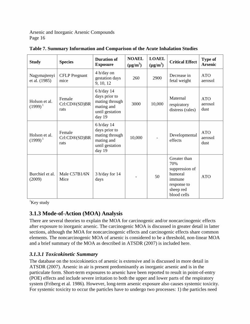
Table 7. Summary Information and Comparison of the Acute Inhalation Studies

Study Species Duration of Exposure

NOAEL (µg/m3)

LOAEL (µg/m3)

Critical Effect Type of Arsenic

Nagymajtenyi et al. (1985)

CFLP Pregnant mice

4 h/day on gestation days 9, 10, 12

260 2900 Decrease in fetal weight

ATO aerosol

Holson et al. (1999) 1

Female Crl:CD®(SD)BR rats

6 h/day 14 days prior to mating through mating and until gestation day 19

3000 10,000 Maternal respiratory distress (rales)

ATO aerosol dust

Holson et al. (1999) 1

Female Crl:CD®(SD)BR rats

6 h/day 14 days prior to mating through mating and until gestation day 19

10,000 - Developmental effects

ATO aerosol dust

Burchiel et al. (2009)

Male C57B1/6N Mice

3 h/day for 14 days - 50

Greater than 70% suppression of humoral immune response to sheep red blood cells

ATO

1Key study

3.1.3 Mode-of-Action (MOA) Analysis There are several theories to explain the MOA for carcinogenic and/or noncarcinogenic effects after exposure to inorganic arsenic. The carcinogenic MOA is discussed in greater detail in latter sections, although the MOA for noncarcinogenic effects and carcinogenic effects share common elements. The noncarcinogenic MOA of arsenic is considered to be a threshold, non-linear MOA and a brief summary of the MOA as described in ATSDR (2007) is included here.

3.1.3.1 Toxicokinetic Summary The database on the toxicokinetics of arsenic is extensive and is discussed in more detail in ATSDR (2007). Arsenic in air is present predominantly as inorganic arsenic and is in the particulate form. Short-term exposures to arsenic have been reported to result in point-of-entry (POE) effects and include severe irritation to both the upper and lower parts of the respiratory system (Friberg et al. 1986). However, long-term arsenic exposure also causes systemic toxicity. For systemic toxicity to occur the particles have to undergo two processes: 1) the particles need


to be deposited onto the lung surface and 2) the deposited particles need to be absorbed from the lung.

The rate of absorption of arsenic is dependent on whether the arsenic is present in the soluble (i.e., arsenate and arsenite) versus insoluble form (i.e., arsenic sulfide, lead arsenate). The soluble forms of arsenic are better absorbed than the insoluble forms for both the inhalation and oral routes of exposure. Also, the toxicity of arsenic compounds is generally associated with soluble inorganic trivalent forms when compared to the pentavalent forms because the pentavalent inorganic compounds have to be first reduced in vivo to the trivalent forms prior to toxicity occurring (Harvey, 1970).

3.1.3.2 Interaction with Sulfhydryl-Containing Enzymes At the cellular level, two mechanisms seem to exist by which inorganic arsenic can elicit toxicity. In the first mechanism, arsenic binds with sulfhydryl groups and disrupts sulfhydryl-containing enzymes. The disruption of these critical enzymes results in an inhibition of a suite of enzyme pathways that includes: inhibition of the pyruvate and succinate oxidation pathways and the tricarboxylic acid cycle, impaired gluconeogenesis, and reduced oxidative phosphorylation. In the second mechanism, arsenic toxicity is thought to occur due to the ability of pentavalent arsenic to substitute for phosphorus in many biochemical reactions. The pentavalent arsenic anion is less stable when compared to the phosphorus anion in phosphate. This results in rapid hydrolysis of high-energy bonds in compounds such as adenosine triphosphate (ATP) and leads to loss of high-energy phosphate bonds and effectively "uncouples" oxidative phosphorylation (ATSDR 2007).

3.1.3.3 Metabolism The toxicity and carcinogenicity of inorganic arsenic is reported to be associated with the metabolic process which is depicted in Figure 1. The metabolism of arsenic involves basically two steps: 1) reduction/oxidation reactions in which the absorbed arsenate (AsV) is reduced rapidly to arsenite (AsIII) 2) methylation to monomethylated arsenic (MMA(V)), reduction to MMA(III), and methylation to MMA(V). ATSDR (2007) indicates these processes to be similar whether exposure is by inhalation, oral, or parenteral route. However, there is some discussion about the methylation step. Some consider the methylation to be a “detoxification” step and others consider it to be an “activation” step. Additional details are included in Section 4.22 (Carcinogenic MOA).

Methylation of arsenite by S-adenosylmethionine (SAM) results in monomethylated arsenic (MMA) and dimethylated arsenic (DMA) the relatively less toxic forms of arsenic. When compared to the inorganic forms of arsenic the methylated forms (i.e., MMA and DMA) react to a lesser extent with tissue constituents and are also readily excreted in the urine. However, some of the intermediates of the methylation process include trivalent metabolites MMAIII and DMAIII. These trivalent metabolites are very reactive, and have been detected in the urine of humans chronically exposed to inorganic arsenic in drinking water. In addition, many in vitro studies have demonstrated both MMAIII and DMAIII have genotoxic and DNA-damaging properties (ATSDR 2007).


It is important to note that the availability of methyl donors (e.g., methionine, choline, cysteine) is different under normal conditions and under severe conditions, such as dietary restrictions. While the availability of methyl donors is not rate-limiting under normal conditions, the methylating capacity can become rate-limiting under severe diet restriction.

Figure 1. Inorganic arsenic biotransformation pathway. SAM, S-adenosylmethionine, SAHC, S-adenosylhomocysteine (Source: Aposhian et al. 2000 as cited in ATSDR 2007)

An alternate biotransformation pathway has been proposed by Hayakawa et al. (2005) and described in ATSDR (2007). This alternate pathway is based on the nonenzymatic formation of glutathione complexes with arsenite resulting in the formation of arsenic triglutathione. According to ATSDR (2007), in the first inorganic arsenic biotransformation pathway, MMA(V) is converted to the more toxic MMA(III). In contrast, in the alternative pathway, MMA(III) is converted to the less toxic MMA(V). ATSDR (2007) did not prefer or select one metabolic pathway over the other. Please refer to ATSDR (2007) for a more detailed description of arsenic metabolism.

According to ATSDR (2007), the Mann model (Gentry et al. 2004, Mann et al. 1996a, 1996b) is a well-derived physiological based pharmacokinetic (PBPK) model consisting of multiple compartments and metabolic processes, and models four chemical forms of arsenic (two organic and inorganic). The Mann model simulates the absorption, distribution, metabolism, elimination, and excretion of As(III), As(V), MMA, and DMA after oral and inhalation exposures in mice,


hamsters, rabbits, and humans. However, the Mann model was not used in the present DSD to perform animal-to-human dosimetric adjustments as it includes both the inhalation and ingestion pathways and does not provide the ability to separately study the inhalation pathway. For a detailed description of PBPK models, please refer to ATSDR (2007).

3.1.3.4 Oxidative Stress Results of in vitro and in vivo studies in human and animals suggest generation of reactive oxygen species as necessary for increased lipid peroxidation, superoxide production, hydroxyl radical formation, and/or oxidant-induced DNA damage. Mechanistic studies exist that support the hypothesis of arsenic-induced oxidative stress and include findings that inhaled arsenic can predispose the lung to oxidative damage and that chronic low-dose arsenic exposure can alter genes and proteins associated with oxidative stress and inflammation.

3.1.4 Dose Metric In the key and the supporting studies, data on the exposure concentration of the parent chemical are available. Since data on other specific dose metrics (e.g., blood concentration of parent chemical, area under blood concentration curve of parent chemical, or putative metabolite concentrations in blood or target tissues) are not available for these studies, exposure concentration of the parent chemical will be used as the default dose metric.

3.1.5 Point of Departure (POD) for the Key Study As the NOAEL for maternal effects (3 mg/m3) is lower than the NOAEL for fetal toxicity (10 mg/m3), the TCEQ used the NOAEL of 3 mg/m3 for the maternal effects as the POD to estimate the acute Rev and acuteESL.

3.1.6 Dosimetric Adjustments

3.1.6.1 Default Exposure Duration Adjustments Reproductive/developmental studies are usually conducted by exposing animals to repeated doses over several days (e.g., 6 h per day for gestational days 6-15). The TD uses a single day of exposure from the experimental study as the exposure duration (TCEQ 2006). In doing so, the TD recognizes that the reproductive/developmental effects may have been caused by only a single day’s exposure that occurred at a critical time during gestation. The critical effect is maternal toxicity (i.e., rales). The concentration (C1) at the 6-h exposure duration (T1) in the key study by Holson et al. (1999) was adjusted to an adjusted POD (PODADJ) concentration (C2) applicable to a 1-h exposure duration (T2) using Haber’s Rule as modified by ten Berge et al. (1986) (C1

n × T1 = C2n × T2) with n = 3, where both concentration and duration play a role in

toxicity. The TCEQ chose to adjust the exposure from 6 h/d to 1 h/d rather than adjusting the total duration of exposure in the study (i.e., 6 h/d for 14 days = 84 h to 1 h) in consideration of protecting against intermittent exposure and the possibility of delayed inflammation.

C2 = [(C

1)3 × (T

1 / T

2)]

1/3 = PODADJ

= [(3 mg/m3)3 × (6 h/1 h)]

1/3 = 5.451 mg/m

3


3.1.6.2 Default Dosimetry Adjustments from Animal-to-Human Exposure Since arsenic in air is primarily in the particulate form (Table 3), and the study was conducted in rats, the Chemical Industry Institute of Toxicology (CIIT) Centers for Health Research and National Institute for Public Health and the Environment (RIVM) 2002 multiple path particle dosimetry model (MPPD) v 2.1 program (CIIT and RIVM 2002) was used to calculate the deposition fraction of ATO in the target respiratory region.

Parameters necessary for this program are particle diameter, particle density, chemical concentration, and target pulmonary region(s). The particle diameter was reported as the MMAD and ranged from 1.9 - 2.2 μm in the Holson study. An average MMAD of 2.07 μm and an average GSD of 1.85 were used in the present analysis. These averages were calculated by considering the data from the three exposures used in the study. The estimated chemical concentration after duration adjustment is the PODADJ of 5.451 mg/m3

and the pulmonary region was considered to be the target region for the particle distribution. The Holson et al. (1999) study reported the rats to have rales, (i.e., labored respiration and gasping) which reflect that the problem is with the alveolar region tissue and airways. Therefore, target region for inorganic arsenic was considered to be the pulmonary region. For the RDDR calculations, the TD used the default minute ventilation (VE) for humans (13,800 mL/min) given by USEPA (1994). Neither USEPA (1994) nor cited USEPA background documents provide the human tidal volume (mL/breath) and breathing frequency (breaths/min) values which correspond to the default USEPA minute ventilation and are needed for input into the MPPD so that both the MPPD model and RDDR calculation use the same human minute ventilation.

Therefore, the TD used human tidal volume and breathing frequency values from de Winter-Sorkina and Cassee (2002) to determine the quantitative relationship between the two and calculate the tidal volume and breathing frequency values corresponding to the default USEPA minute ventilation for input into the MPPD model (Appendix A2). The calculated human tidal volume is 842.74 ml/breath and the breathing frequency is 16.375 breaths per minute. Except for the parameter values discussed above, all remaining values used were default.

Once the total particle distribution was determined (Appendix A1 and A2), the Regional Deposition Dose Ratio (RDDR) was calculated as follows:

𝑅𝐷𝐷𝑅 =(𝑉E)𝐴(𝑉E)H

×𝐷𝐹𝐴𝐷𝐹H

×𝑁𝐹H

𝑁𝐹A

where: VE = minute volume DF = deposition fraction in the target region of the respiratory tract NF = normalizing factor A =animal H = human


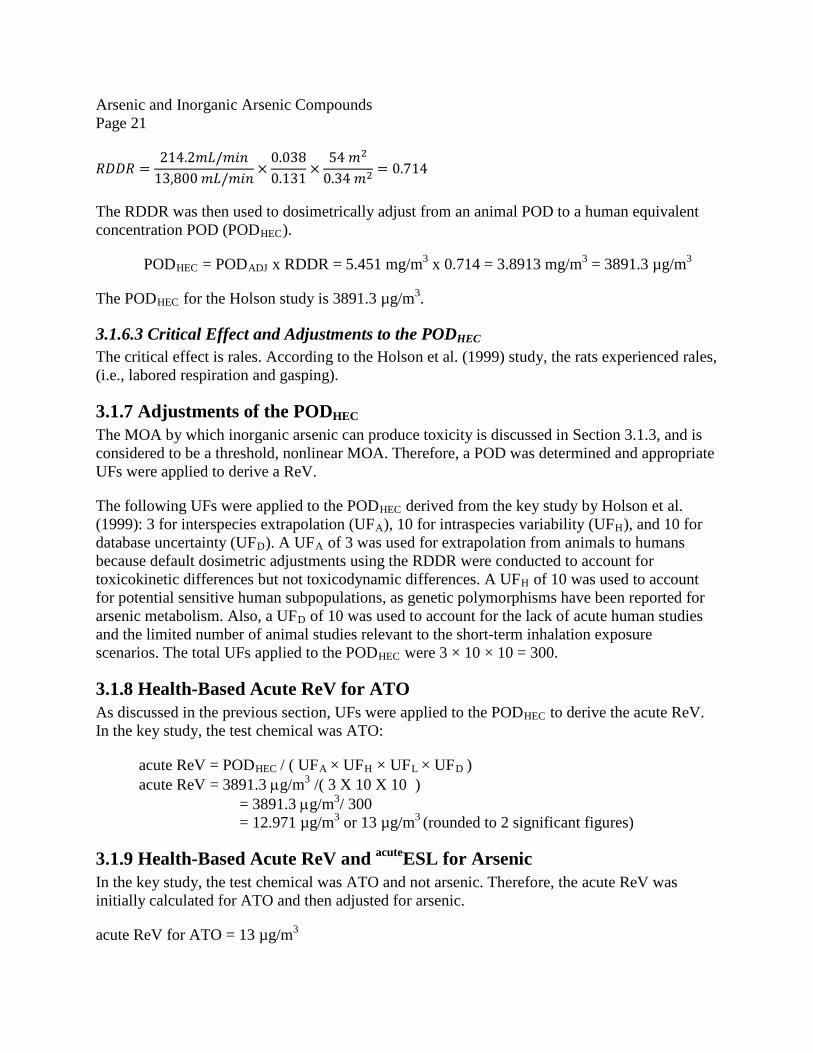
𝑅𝐷𝐷𝑅 =214.2𝑚𝐿/𝑚𝑖𝑛

13,800 𝑚𝐿/𝑚𝑖𝑛×

0.0380.131

×54 𝑚2

0.34 𝑚2 = 0.714

The RDDR was then used to dosimetrically adjust from an animal POD to a human equivalent concentration POD (PODHEC).

PODHEC = PODADJ x RDDR = 5.451 mg/m3 x 0.714 = 3.8913 mg/m3 = 3891.3 µg/m3

The PODHEC for the Holson study is 3891.3 µg/m3.

3.1.6.3 Critical Effect and Adjustments to the PODHEC The critical effect is rales. According to the Holson et al. (1999) study, the rats experienced rales, (i.e., labored respiration and gasping).

3.1.7 Adjustments of the PODHEC The MOA by which inorganic arsenic can produce toxicity is discussed in Section 3.1.3, and is considered to be a threshold, nonlinear MOA. Therefore, a POD was determined and appropriate UFs were applied to derive a ReV.

The following UFs were applied to the PODHEC derived from the key study by Holson et al. (1999): 3 for interspecies extrapolation (UFA), 10 for intraspecies variability (UFH), and 10 for database uncertainty (UFD). A UFA of 3 was used for extrapolation from animals to humans because default dosimetric adjustments using the RDDR were conducted to account for toxicokinetic differences but not toxicodynamic differences. A UFH of 10 was used to account for potential sensitive human subpopulations, as genetic polymorphisms have been reported for arsenic metabolism. Also, a UFD of 10 was used to account for the lack of acute human studies and the limited number of animal studies relevant to the short-term inhalation exposure scenarios. The total UFs applied to the PODHEC were 3 × 10 × 10 = 300.

3.1.8 Health-Based Acute ReV for ATO As discussed in the previous section, UFs were applied to the PODHEC to derive the acute ReV. In the key study, the test chemical was ATO:

acute ReV = PODHEC / ( UFA × UFH × UFL × UFD ) acute ReV = 3891.3 µg/m3

/( 3 X 10 X 10 ) = 3891.3 µg/m3/ 300 = 12.971 µg/m3 or 13 µg/m3 (rounded to 2 significant figures)

3.1.9 Health-Based Acute ReV and acuteESL for Arsenic In the key study, the test chemical was ATO and not arsenic. Therefore, the acute ReV was initially calculated for ATO and then adjusted for arsenic.

acute ReV for ATO = 13 µg/m3


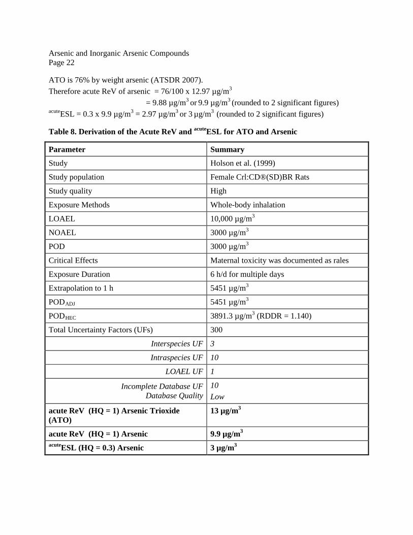
ATO is 76% by weight arsenic (ATSDR 2007). Therefore acute ReV of arsenic = 76/100 x 12.97 µg/m3

= 9.88 µg/m3 or 9.9 µg/m3 (rounded to 2 significant figures)

acuteESL = 0.3 x 9.9 µg/m3 = 2.97 µg/m3 or 3 µg/m3 (rounded to 2 significant figures)

Table 8. Derivation of the Acute ReV and acuteESL for ATO and Arsenic

Parameter Summary

Study Holson et al. (1999)

Study population Female Crl:CD®(SD)BR Rats

Study quality High

Exposure Methods Whole-body inhalation

LOAEL 10,000 µg/m3

NOAEL 3000 µg/m3

POD 3000 µg/m3

Critical Effects Maternal toxicity was documented as rales

Exposure Duration 6 h/d for multiple days

Extrapolation to 1 h 5451 µg/m3

PODADJ 5451 µg/m3

PODHEC 3891.3 µg/m3 (RDDR = 1.140)

Total Uncertainty Factors (UFs) 300

Interspecies UF 3

Intraspecies UF 10

LOAEL UF 1

Incomplete Database UF Database Quality

10 Low

acute ReV (HQ = 1) Arsenic Trioxide (ATO)

13 µg/m3

acute ReV (HQ = 1) Arsenic 9.9 µg/m3 acuteESL (HQ = 0.3) Arsenic 3 µg/m3


3.1.10 Comparison of Results The database on the acute effects of arsenic via inhalation exposure is limited. The USEPA does not have a Reference Concentration (RfC) and ATSDR does not have a Minimal Risk Level (MRL) via inhalation exposure for inorganic arsenic. Cal EPA developed an acute Reference Exposure Level (REL) for inorganic arsenic of 0.2 µg/m3 (December 2008) and used the mice study by Nagymajtenyi et al. (1985) as the key study. The critical effect was decreased fetal weight in mice. The TCEQ’s acuteESL (3 µg/m3) is based on the Holson et al. (1999) study in which no reproductive/developmental effects were reported. In the Holson study, maternal toxicity, as evidenced by the occurrence of rales during pre-mating and gestation exposure, was observed only at the high dose.

3.2 Welfare-Based acuteESLs

3.2.1 Odor Perception Elemental arsenic is odorless (ATSDR 2007). No odor data were available for arsenic or inorganic arsenic compounds.

3.2.2 Vegetation Effects No data on vegetative effects were found due to exposure to inorganic arsenic in the ambient air. While organic arsenicals have been used as pesticides and defoliants on cotton plants, no data was available on the adverse vegetative effects from organic arsenic in ambient air. The TD will evaluate the vegetation effects on exposure to inorganic arsenic in ambient air as new studies and/or data becomes available.

3.3 Short-Term ESL and Values for Air Monitoring Evaluation The acute evaluation resulted in the derivation of the following values for arsenic:

• acute ReV = 9.9 µg/m3

• acuteESL = 3 µg/m3

The acute ReV of 9.9 µg/m3will be only used for the evaluation of air monitoring data (Table 1). The short-term ESL for air permit reviews is the health-based acuteESL of 3 µg/m3 (Table 2). The health-based acuteESL is only for air permit reviews, and not for the evaluation of ambient air monitoring data. If the predicted 1-h maximum ground level concentration (GLCmax) is equal to or less than the health-based acuteESL, then no acute health effects would be expected.


Chapter 4 Chronic Evaluation

4.1 Noncarcinogenic Potential

4.1.1 Physical/Chemical Properties Physical/chemical properties of arsenic and inorganic arsenic compounds have been previously discussed in Chapter 3, Section 3.1.1. Only a few chronic animal inhalation studies exist. Many of the available animal studies are for the oral ingestion route and will not be discussed here. Refer to ATSDR (2007) for a discussion of animal studies. While chronic inhalation exposure to inorganic arsenicals has been reported to cause neurological effects in humans, no characteristic neurological symptoms were reported in monkeys, dogs, or rats that were chronically exposed to inorganic arsenicals at doses of 0.7 - 2.8 mg As/kg/day (EPA 1980 as cited in ATSDR 2007). ATSDR (2007) attributes the lack of chronic response in these animal studies to insufficient exposure duration and/or small sample sizes.

The TD will use human data to derive chronic toxicity factors and will mainly use the ATSDR (2007) review of arsenic to discuss and determine the chronic ReV and ESL for inorganic arsenic.

4.1.2 Key Human Studies

4.1.2.1 Vascular and Cardiovascular Effects Long-term exposure to arsenic in drinking water has been reported to cause vascular effects (e.g., gangrene or black foot disease) (Lagerkvist et al. 1986). Evidence from epidemiological studies indicates cardiovascular effects may also occur after long-term exposure to inhaled arsenic. Blom et al. (1985) and Lagerkvist et al. (1986, 1988) conducted cross-sectional studies of workers exposed to ATO dust in the Ronnskar smelter in northern Sweden to discern changes in peripheral circulation via sensitive physiological methods.

Urinary arsenic metabolite measurements have been routinely used in occupational exposure studies as a means to monitor exposure to arsenic (Vahter 1986). However, Pinto et al. (1976) and others have reported a weak correlation between airborne arsenic and the total concentration of arsenic in urine. One of the explanations for this lack of correlation is that urinary arsenic is greatly influenced by the amount of seafood consumed by the arsenic workers, since fish and certain crustaceans contain high concentrations of organic arsenic (e.g., arsenobetaine).

Brief summaries of the Lagerkvist and Zetterlund (1994), Lagerkvist et al. (1986), and Blom et al. (1985) studies are included as they indicate chronic arsenic toxicity. However, because of limited exposure information, the TCEQ did not calculate quantitative estimates of chronic toxicity to determine the chronic ReV and the chronic ESL for non-carcinogenic effects (chronicESLnonlinear(nc)). It is to be noted that both Lagerkvist and Zetterlund (1994), and the Lagerkvist et al. (1986) studies were follow-up studies of the Blom et al. (1985) study.


Therefore, the TCEQ will first discuss the Blom et al. (1985) study and then discuss the other two studies.

4.1.2.1 Blom et al. (1985) Blom et al. (1985) examined peripheral nervous function in copper and lead smelter workers chronically exposed to airborne arsenic for 8 - 40 years (mean 23 years). A total of 47 workers from the Ronnskar copper smelter were selected as the arsenic-exposed group. While an additional 15 workers were employed in the smelter, they were not included in the study because they were diagnosed as having chronic illness unrelated to arsenic exposure and/or because they declined to participate in the study. In addition to arsenic exposure, the workers at the smelter were exposed to sulfur dioxide and heavy metals such as gold, silver, copper, and lead.

The controla group included 50 workers from a mechanical industrial enterprise located in the same county as the arsenic workers, and were matched to the arsenic workers by age, use of tobacco, and use of vibrating tools. Vibrating tools have been considered as a risk factor for developing neurological symptoms. Both the exposed group and the control group were screened for pre-existing medical conditions such as diabetes and peripheral vascular disease.

Blom et al. (1985) estimated the arsenic concentration in the air at the smelter to be below 500 µg/m3 before 1975 and about 50 µg/m3 after 1975. The workers underwent a thorough clinical and physical examination. Toe and finger plethysmography (a test used to measure changes in blood flow or air volume in different parts of the body to check for blood clots in the arms and legs or to measure how much air can be held in the lungs) was performed with a mercury strain gauge in a warm room at a skin temperature of about 30º C. Systolic blood pressure (BP) in the fingers after cooling was measured. In addition, the BP in the arm was measured with the cuff method and a BP difference of 40 mm between arm and digit was taken as a sign of arterial obstruction.

Finger systolic pressure (FSP) was measured simultaneously in two fingers of the same hand and expressed as a percentage. While a decrease in BP occurs after cooling in normal subjects, the decrease becomes more pronounced in subjects with peripheral damage as observed in subjects with Raynaud’s phenomenon, a peripheral vascular disease characterized by spasm of digital arteries and numbness of the fingers.

The mean urinary arsenic level in the exposed group was reported to be 71 µg/L. According to Blom et al. (1985) urinary arsenic levels greater than 71 µg/L were generally associated with clinical neuropathy in previous studies. In the present study, minor neurological and electromyographic abnormalities were reported among the arsenic workers with mean urinary

a The terms “referent” and “control” will be used intermittently throughout the DSD and will refer to unexposed workers.


arsenic concentrations of 71 µg/L. A slightly reduced nerve conduction velocity (NCV) in two or more peripheral nerves was reported among the exposed group of arsenic workers when compared to the referent population (control group). In regards to chronic arsenic exposure, a statistically significant correlation was reported for cumulative arsenic exposure and reduced NCV in five peripheral motor nerves. Blom et al. (1985) hypothesized the reduction in the NCV was a sign of subclinical neuropathy and indicated that detection of these subclinical changes could help prevent the onset of other adverse health effects due to chronic arsenic exposure. The Blom et al. (1985) study was not chosen as a key study due to the availability of more recent smelter data, which are discussed in the following sections (Lagerkvist et al. 1986; Lagerkvist and Zetterlund 1994).

4.1.2.1.2 Lagerkvist and Zetterlund (1994) A total of 43 male workers and 46 referents previously examined by Blom et al. (1985) were re-examined by Lagerkvist and Zetterlund (1994). In the study, the arsenic-exposed workers from the Blom et al. (1985) study were exposed to arsenic dust while working at the smelter for an additional five years. Therefore, the duration of arsenic exposure as ATO in the follow-up study ranged from 13 - 45 years with mean exposure duration of 28 years. Since the collection of the Blom data, one of the arsenic workers and two of the referents died of heart infarction and another referent died of liver cancer. Two other arsenic workers retired or did not want to participate in the study. One of the arsenic workers was excluded from the study as he was diagnosed with hereditary polyneuropathy (i.e., reduced NCV).

As the Lagerkvist and Zetterlund (1994) study is a follow-up to the Blom et al. (1985) study, the estimated arsenic levels in the air were adjusted for an additional five years of exposure. The arsenic levels at the smelter were reported to be 500 µg/m3 from 1950’s to 1975 (mean of 16 years), 50 µg/m3 from 1975 to 1987 (mean of 11 years), and 30 µg/m3 from 1987 (one year).

Previous studies had identified the average particle size of the airborne dust at the smelter to be about 5 µm (Leffler et al. 1984 as cited in Lagerkvist and Zetterlund 1994). In the study, the mean total estimated absorption of arsenic for the arsenic workers was reported to be 25 mg per year. The exposed and control groups were compared for differences using two-tailed Student’s test, chi-square test, or the Fisher’s exact probability test. In addition, the correlation coefficients were calculated with Spearman’s rank correlation and regression equations between variables with the method of least squares (Colton 1974, Siegel 1956).

While the arsenic-exposed workers were examined for a period of five years from 1982 - 1987, the results were extrapolated to long-term exposure with a mean duration of 28 years as the arsenic workers and referents were re-examined from the Blom et al. (1985) study. The general health of the arsenic-exposed workers was poor and they reported a larger number of symptoms than the referents. The authors attributed the poor health of the arsenic workers to exposure to inorganic arsenic. In addition, four of the arsenic workers were reported to be diagnosed as having diabetes during the follow-up period while none of the referents were diagnosed as having diabetes. There is increasing evidence that inorganic arsenic can adversely affect glucose


metabolism in humans via oral ingestion. However, there is only limited evidence in regards to inhalation exposure to inorganic arsenic and diabetes in humans.

Similar to the Blom et al. (1985) study, reduction in the NCV was studied to determine peripheral nerve function both in the arsenic workers (exposed) and referent (control) groups. There were increased differences in the NCV between the arsenic workers and controls in all the examined nerves, with the greatest difference in the tibial and the sural nerves when examined from 1982-1987. However, the nerves in the arm seemed to be less affected. Further, in both the Blom et al. (1985) and the Lagerkvist and Zetterlund (1994) studies, there was a significant negative correlation between the estimated total arsenic absorption and NCV’s in the peripheral nerves. According to ATSDR (2007), the time-weighted average (TWA) exposure for arsenic (as ATO) based on the Lagerkvist and Zetterlund (1994) study was calculated as follows:

�500 𝜇𝑔𝑚3 × 16 𝑦𝑒𝑎𝑟𝑠� + �50 𝜇𝑔𝑚3 × 11𝑦𝑒𝑎𝑟𝑠�+ �30 𝜇𝑔𝑚3�

28 𝑦𝑒𝑎𝑟𝑠

=8580 𝜇𝑔𝑚3

28 𝑦𝑒𝑎𝑟𝑠= 306.43

𝜇𝑔𝑚3 �0.306

𝑚𝑔𝑚3�

The prevalence of abnormally low NCV remained significantly increased in the exposed workers in the follow-up study, and the decrease in mean NCV was also statistically significant in the tibial (motor) and sural (sensory) nerves. Based on the Lagerkvist and Zetterlund (1994) study, ATSDR (2007) estimated a LOAEL of 306.43 µg/m3 (0.306 mg/m3) for decreased NCV.

In addition to peripheral neuropathy, the arsenic-exposed workers were reported to have clinical manifestations of neuropathy (i.e., numbness, parasthesia, or muscle pain) that were significantly different from the referents. Similar results were reported by Oh (1991), who reported a marked decrease in sensory nerve conduction both in the acute and in the moderate stage of recovery from neuropathy even after nine years since exposure to inorganic arsenic.

4.1.2.1.3 Lagerkvist et al. (1986) As already mentioned, the Lagerkvist et al. (1986) study appears to be very similar to the Blom et al. (1985) study in many aspects such as the location (i.e., Ronnskar smelter in Sweden), the exposure duration, and the number of exposed workers. Only the number of control workers in the Blom et al. (1985) study and the Lagerkvist et al. (1986) are different. As a detailed discussion was already provided in the Blom et al. (1985) study, only the aspects that are different will be explained in this section.

Lagerkvist et al. (1986) reported the mean exposure duration for arsenic workers to be 23 years, of which they estimated that for 16 years the exposure was at 500 µg As/m3 and for seven years the exposure was at 50 µg As/m3. ATSDR (2007) estimated a time-weighted average (TWA) for inorganic arsenic exposure as follows:


�500 𝜇𝑔𝑚3 × 16 𝑦𝑒𝑎𝑟𝑠� + �50 𝜇𝑔𝑚3 × 7 𝑦𝑒𝑎𝑟𝑠�23 𝑦𝑒𝑎𝑟𝑠 =

8350 𝜇𝑔𝑚3

23 𝑦𝑒𝑎𝑟𝑠

= 363 𝜇𝑔 𝐴𝑠𝑚3 �0.363

𝑚𝑔 𝐴𝑠𝑚3 �

ATSDR (2007) reported that a cross-sectional study of workers exposed to an estimated TWA of 0.36 mg As/m3 at the Ronnskar copper smelter in Sweden for an average of 23 years showed that the smelter workers had significantly increased incidences of Raynaud’s phenomenon and showed increased vasospasticity (constriction of blood vessels) in response to cold when tested in the fingers (Lagerkvist et al.1986). A follow-up study by Lagerkvist et al. (1988) indicated vasospasticity measurements to improve when exposure to arsenic was reduced. However, the symptoms of peripheral vascular effects (cold hands or feet, white fingers, numbness in fingers or feet) still persisted even after reduction in exposure.

The LOAEL for Raynaud’s phenomenon and vasospasticity was estimated by ATSDR (2007) from the Lagerkvist et al. (1986) study to be 0.36 mg As/m3. The Raynaud’s phenomenon and increased vasospaticity are considered cardiovascular effects (ATSDR 2007).

4.1.2.2 Respiratory, Ocular, Dermal, and Gastrointestinal Effects Although it has been established that inorganic arsenic dust is an irritant, relatively few systemic studies have been conducted. Respiratory, ocular, and gastrointestinal effects have been reported due to inhalation exposure. However, the available studies are limited due to small sample sizes, inadequate exposure concentrations, and the inability to relate exposure concentrations to specific health effects. This is especially true for ocular and gastrointestinal effects. For that reason, only a brief discussion of ocular and gastrointestinal effects as reviewed in ATSDR (2007) will be included in this DSD and a more detailed discussion of the respiratory and dermal effects will be included. Respiratory effects can also occur due to short-term exposure to arsenic as discussed previously in Section 3.1.2.2.1.

Workers exposed to arsenic dust in air have been reported to have experienced laryngitis, bronchitis, rhinitis (Dunlap 1921, Pinto and McGill, 1953, and Sandstorm et al. 1989 as cited in ATSDR 2007), and chemical conjunctivitis (i.e., redness, swelling and pain in the eyes (Dunlap 1921 as cited in ATSDR 2007)).

While gastrointestinal effects are normally associated with arsenic exposure via oral ingestion (Pinto and McGill as cited in ATSDR 2007), case reports from workers occupationally exposed to arsenic dust reported nausea, vomiting, and diarrhea. According to ATSDR (2007), it is possible that mucociliary transport of arsenic dust from the lungs to the gut could be responsible for the effects.

4.1.2.2.1 Perry et al. (1948) Perry et al. (1948) conducted a cross-sectional study to investigate a factory where workers were exposed to arsenic dust during preparation and packing of sodium arsenite powder. All the


workers underwent a thorough clinical examination. The duration of exposure for most workers ranged from 0.5 - 50 years. The workers in the high exposure group were reported to be exposed to arsenic dust in the range of 0.384 - 1.034 mg As/m3 with an estimated average exposure of 0.613 mg As/m3. Workers in the lower exposure group were estimated to be exposed to an average of 0.078 mg As/m3.

Dermal Effects

The workers in the high exposure group were reported to be grossly pigmented with hyperkeratinization of the exposed skin and multiple warts. Workers in the lower exposure group were also reported to have a higher incidence of pigmentation keratosis when compared to the control group. Therefore, the LOAEL from this study for dermal effects is 0.078 mg As/m3. No NOAELs was reported for dermal effects.

Respiratory Effects

In addition to dermal effects, Perry et al. (1948) compared differences in chest x-rays and/or respiratory performance (i.e., vital capacity and exercise-tolerance tests) amongst control and exposed worker groups and reported no differences. Based on the results of this study, ATSDR (2007) has estimated a NOAEL of 0.613 mg As/m3 for respiratory effects.

Although it provided estimated exposure doses, the Perry et al. (1948) study did not include adequate quantitative dose-response information. Therefore, the TD did not consider it as a key study.

4.1.2.2.2 Lubin et al. (2000) Lubin et al. (2000), Lee-Feldstein (1983), and others have investigated the relative risks of non-cancer outcomes due to exposure to airborne arsenic in cohort studies. Lubin et al. (2000) analyzed the increased risk of mortality due to respiratory disease (e.g., emphysema) for arsenic-exposed workers by duration of employment with varying arsenic exposure (i.e, light, medium, and heavy). There were elevated Standard Mortality Ratios (SMR) among workers and former workers last exposed at age 50 years and over for non-malignant respiratory diseases.

While an increased risk was observed with increased duration of employment, the gradients of risk were reported to be similar for all the work areas (i.e., light, medium, and heavy). Lubin et al. (2000) attributed the increasing relative risk of death due to non-malignant respiratory diseases to factors other than arsenic exposure (e.g., smoking). Similar conclusions were reported by Lee-Feldstein (1983 as cited in ATSDR 2007).

4.1.2.3 Neurological Effects Several epidemiology studies indicate that inorganic arsenic is potentially neurotoxic. Long-term exposure to inorganic arsenic has been reported to adversely affect the peripheral nervous system (WHO 1981, Feldman et al. 1979). A few key neurological studies will be discussed in more detail.


4.1.2.3.1 Feldman et al. (1979) Peripheral neuropathy has been reported in copper smelter workers at the ASARCO smelter in Tacoma, Washington (Feldman et al. 1979). A high prevalence of clinical and subclinical neuropathy in smelter workers was found to be associated with high urinary arsenic levels (250 µg/l). While the clinically diagnosed peripheral neuropathy was higher in the arsenic-exposed workers than in the unexposed workers at the ASARCO plant, the differences were not statistically significant (Feldman et al. 1979).

Specifically, Feldman et al. (1979) reported intracellular damage to peripheral neurons resulting in distal axonopathy as a primary effect on long-term exposure to inorganic arsenic with segmental demyeliniation reported as a secondary effect. In general, damage to the sensory nerves was reported prior to any damage to the motor nerves, damage was reported in the distal parts of the extremities, and recovery following cessation of arsenic exposure was very slow. However, the studies were limited as an adequate dose-response relationship was not reported.

4.1.2.3.2 Buchancova et al. (1998) Buchancova et al. (1998) reported peripheral neurological effects due to ATO exposure in power plant workers in Slovakia. The average length of exposure of the power plant workers was 22.3 years and the average concentration of arsenic in the air ranged from 4.6 - 142.7 µg/m3.

4.1.3 MOA Analysis The MOA by which arsenic may produce toxicity is discussed in Section 3.1.3.

4.1.4 Dose Metric Not Applicable.

4.1.5 PODs for Key Studies Not Applicable.

4.1.6 Health-Based Chronic ReV for ATO The TCEQ has included the estimated LOAELs as described in the ATSDR (2007) toxicological profile. However, the TCEQ is of the opinion that the estimated LOAELs include a large amount of uncertainties because of inadequate exposure information. Therefore, the TCEQ will not derive a chronic ReV and chronic ESL for non-carcinogenic effects (chronicESLnonlinear(nc)). The TCEQ will however, derive quantitative estimates for carcinogenic effects (chronicESLlinear(c)) in the latter sections of this DSD. Based on the WOE, the TCEQ is of the opinion that the chronicESLlinear(c) will protect against both the carcinogenic and chronic non-carcinogenic effects.


4.2 Carcinogenic Potential

4.2.1 Weight of Evidence (WOE) Evaluation Several epidemiological studies have been reported in arsenic-exposed smelter workers that indicate that inhalation exposure to inorganic arsenic increases the risk of lung cancer. In 2007, ATSDR conducted a review of the WOE from many of the epidemiological studies and concluded that chronic inhalation exposure to inorganic arsenic increases the risk of lung cancer. In the following sections, the TCEQ staff has included selected portions of Section 3.2.1.7 of ATSDR (2007), with table references removed. In addition to the ATSDR’s review of inorganic arsenic, the TCEQ staff reviewed the individual journal articles referenced in the ATSDR (2007) review and further conducted a thorough review of peer-reviewed articles of inorganic arsenic in regards to inhalation exposure in smelters published after 2007 and included a review of those studies.

Standard mortality rates (SMRs) are often reported in epidemiological studies. A SMR is basically the number of observed deaths due to a particular disease (e.g., lung cancer) in a group divided by the number that would be expected had the group developed the disease at the same rate as a standard population (e.g., unexposed group, general population), taking into account the number of person-years (PY) in each age group of a cohort and age group rates in the standard population.

4.2.1.1 WOE from Epidemiological Studies Included in ATSDR (2007) For the WOE from ATSDR (2007), section headings have been inserted by the TCEQ to separate the discussions of the separate studies. See ATSDR (2007) for the cited references.

4.2.1.1.1 Overview “There is convincing evidence from a large number of epidemiological studies that inhalation exposure to inorganic arsenic increases the risk of lung cancer. Most studies involved workers exposed primarily to arsenic trioxide dust in air at copper smelters (Axelson et al. 1978; Brown and Chu 1982, 1983a, 1983b; Enterline and Marsh 1982; Enterline et al. 1987a, 1987b, 1995; Ferreccio et al. 1996; Järup and Pershagen 1991; Järup et al. 1989; Lee and Fraumeni 1969; Lee-Feldstein 1983, 1986; Lubin et al. 2000; Mazumdar et al. 1989; Pinto et al. 1977, 1978; Sandstrom et al. 1989; Viren and Silvers 1999; Wall 1980; Welch et al. 1982) and mines (Liu and Chen 1996; Qiao et al. 1997; Taylor et al. 1989; Xuan et al. 1993), but increased incidence of lung cancer has also been observed at chemical plants where exposure was primarily to arsenate (Bulbulyan et al. 1996; Mabuchi et al. 1979; Ott et al. 1974; Sobel et al. 1988). In addition, several studies suggest that residents living near smelters or arsenical chemical plants may also have increased risk of lung cancer (Brown et al. 1984; Cordier et al. 1983; Matanoski et al. 1981; Pershagen 1985), although the increases are small and are not clearly detectable in all cases (e.g., Frost et al. 1987). The strongest evidence that arsenic is responsible for the


observed lung cancer comes from quantitative dose-response data relating specific arsenic exposure levels to lung cancer risk. These data are available for arsenic-exposed workers at the ASARCO copper smelter in Tacoma, Washington (Enterline and Marsh 1982; Enterline et al. 1987a, 1995; Mazumdar et al. 1989), the Anaconda copper smelter in Montana (Lee-Feldstein 1986; Welch et al. 1982), eight other US copper smelters (Enterline et al. 1987b), and the Ronnskar copper smelter in Sweden (Järup and Pershagen 1991; Järup et al. 1989). A common limitation of these studies is confounding exposure to other chemicals, such as sulfur dioxide, and cigarette smoking.”

4.2.1.1.2 ASARCO Copper Smelter in Tacoma, Washington “Enterline and Marsh (1982) reported a significant increase in respiratory cancer mortality (standard mortality ratio [SMR]=189.4) based on 104 observed respiratory cancer deaths and only 54.9 expected over the years 1941-1976 in a cohort of 2,802 male workers employed for ≥ 1 year between 1940 and 1964 at the ASARCO smelter. When the cohort was separated into low and high arsenic exposure groups, with mean estimated time-weighted average arsenic exposures of 0.054 and 0.157 mg As/m3, respectively (based on work history, historical urinary arsenic measurements, and an experimentally derived relationship between urinary and inhaled arsenic), respiratory cancer mortality was significantly increased in both groups in a concentration-related fashion (SMR = 227.7 and 291.4 in the low and high groups, respectively). Enterline et al. (1987a) re-analyzed these data using improved exposure estimates that incorporated historical measurements of arsenic in the ambient air and personal breathing zone of workers. Respiratory cancer mortality was significantly increased in a concentration-related fashion in the low (SMR = 213.0), medium (SMR = 312.1), and high (SMR = 340.9) arsenic exposure groups, which had mean estimated time-weighted average arsenic exposures of 0.213, 0.564, and 1.487 mg As/m3, respectively. An alternative analysis of these data by Mazumdar et al. (1989) produced similar results. Enterline et al. (1995) extended the mortality follow-up from 1976 to 1986, but reported findings similar to the earlier study in a less thorough analysis.”

4.2.1.1.3 Anaconda Copper Smelter in Montana “Respiratory cancer mortality was significantly increased (SMR = 285) based on 302 observed respiratory deaths between 1938 and 1977 in a cohort of 8,045 white male workers employed for at least 1 year between 1938 and 1956 at the Anaconda smelter (Lee-Feldstein 1986). When workers were categorized according to cumulative arsenic exposure and date of hire, lung cancer mortality was significantly increased in all groups hired between 1925 and 1947. Workers in the lowest cumulative exposure group (<10 mg-mo/m3) were reported to have had < 2 years of exposure at an average arsenic concentration of 0.38 mg/m3. An alternative analysis of a subset of the Anaconda cohort


(n=1,800, including all 277 employees with heavy arsenic exposure and 20% of the others) that included information on smoking and other occupational exposures was performed by Welch et al. (1982). This analysis showed that lung cancer mortality increased with increasing time-weighted average arsenic exposure, with a small nonsignificant increase in the low group (SMR = 138) exposed to 0.05 mg/m3 and significant increases in the medium (SMR = 303), high (SMR = 375), and very high (SMR = 704) groups exposed to 0.3, 2.75, and 5.0 mg/m3, respectively. Cohort members were more likely to be smokers than US white males, but smoking did not differ among the arsenic exposure groups. Exposure-response analysis of smokers was similar to the analysis based on the full subcohort, while analysis of nonsmokers (limited by small group sizes) also showed a similar pattern, but with lower SMRs. In a followup analysis of the same cohort, Lubin et al. (2000) re-weighted the exposure concentrations based on duration and time of exposure and re-evaluated the effects of exposure. Relative risks for respiratory cancer increased with increasing duration in each arsenic exposure area (light, medium, and heavy) after adjustment for duration in the other two exposure areas. SMRs were significantly elevated following exposure to 0.58 mg/m3 (medium; SMR = 3.01, 95% CI = 2.0-4.6) or 11.3 mg/m3 (high; SMR = 3.68, 95% CI = 2.1-6.4) for 10 or more years, and following exposure to 0.29 mg/m3 (low; SMR = 1.86, 95% CI=1.2-2.9) for 25 or more years.”

4.2.1.1.4 Eight US Copper Smelters “Enterline et al. (1987b) studied the mortality experience from 1949 to 1980 of a cohort of 6,078 white males who had worked for 3 years or more between 1946 and 1976 at one of eight US copper smelters in Arizona, Utah, Tennessee, and Nevada. Lung cancer mortality was significantly increased only in the Utah smelter (SMR = 226.7), which had the highest average arsenic exposure concentration (0.069 mg/m3 vs. 0.007-0.013 mg/m3 in the other smelters) and also contributed the largest number of cohort members (n=2,288 vs. 189-965 from the other smelters). A nested case-control study showed that arsenic exposure and cigarette smoking were significant risk factors for lung cancer in the smelter workers. Smoking was lower in the Utah smelter workers than in the other smelter workers, but still higher than in the referent Utah population, suggesting that the risk attributable to arsenic in this study population is somewhat lower than indicated by the SMR reported above.”

4.2.1.1.5 Ronnskar Copper Smelter in Sweden “Järup et al. (1989) reported significantly increased lung cancer mortality (SMR = 372, 95% confidence interval [CI] = 304-450) based on 106 lung cancer deaths in a cohort of 3,916 male workers employed for ≥ 3 months between 1928 and 1967 at the Ronnskar smelter and followed for mortality through 1981. Workers were separated into low, medium, and high arsenic


exposure groups with mean time-weighted average exposure estimates of 0.05, 0.2, and 0.4 mg/m3, respectively. Lung cancer mortality was significantly increased in all three exposure groups in a concentration-related fashion (SMR = 201, 353, and 480, respectively). A nested case-control analysis of 102 lung cancer cases and 190 controls from the cohort showed that lung cancer risk increased with increasing arsenic exposure in nonsmokers, light smokers, and heavy smokers (Järup and Pershagen 1991). The results demonstrated that arsenic is a risk factor for lung cancer in the smelter workers, but also suggested a greater-than-additive interaction between smoking and arsenic exposure. In this analysis, in contrast to the cohort study, lung cancer risk due to arsenic was increased only in the higher arsenic-exposure groups. Potential explanations for this difference between the cohort and case-control analyses include a higher proportion of smokers in the smelter workers than in the regional referent population in the cohort study, and limited power to detect increased risk in the case-control study due to small group sizes in the dose-response analysis.”

4.2.1.1.6 Other Types of Nonrespiratory Cancer “There have been occasional reports of other types of cancer (i.e., nonrespiratory cancer) potentially associated with inhalation exposure to inorganic arsenic, but there is no strong evidence for any of them. For example, Enterline et al. (1995) found significantly increased mortality due to cancer of the large intestine and bone cancer in the ASARCO cohort. However, neither cancer showed any relation to cumulative arsenic exposure, and the purported increase in bone cancer risk was based on a very small number of observations. Pesch et al. (2002) reported an increase in nonmelanoma skin cancers resulting from exposure from a Slovakian coal-burning power plant, but exposure levels associated with the lesions were not presented. Bencko et al. (2005) also reported an increase in the incidence of nonmelanoma skin cancer among workers of a power plant burning coal of a high arsenic content and in the population living in the vicinity of the power plant. Bulbulyan et al. (1996) reported an increase in risk of stomach cancer among workers exposed to the highest average arsenic concentrations at a Russian fertilizer plant, but this finding, which was based on a small number of observations and was only marginally statistically significant, was confounded by exposure to nitrogen oxides, which were more convincingly associated with stomach cancer in this study. Wingren and Axelson (1993) reported an association between arsenic exposure and stomach and colon cancer in Swedish glass workers, but this result was confounded by concomitant exposure to other metals. Lee-Feldstein (1983) observed a small, marginally significant increase in digestive tract cancer (SMR = 125) in one study of the Anaconda cohort, but this was not found in other studies of this cohort (Lee and Fraumeni 1969; Lee-Feldstein 1986; Welch et al. 1982). Wulff et al. (1996) observed an apparent increase in


the risk of childhood cancer (all types combined) in the population living within 20 km of the Ronnskar smelter, but the apparent increase was based on a small number of cases (13 observed vs. 6.7 expected) and was not statistically significant, and exposure to arsenic was confounded by exposure to lead, copper, cadmium, sulfur dioxide, and possibly other emissions such as arsenic and selenium. A retrospective study of deaths due to unspecified types of malignancies among workers of power plants found no significant differences in death rate between two groups whose exposure levels to arsenic had a difference of one order of magnitude (Bencko et al. 1980). However, the mean age of those deceased due to cancer in the high-exposure group was 55.9 years compared to 61.2 years in the low-exposure group, and this difference was statistically significant (p<0.05). Also, when the workers were stratified by exposure-duration, there was a significantly higher frequency of tumors in the high-exposure group after shorter employment periods (<5 or 6-10 years) than after a longer employment period (≥11 years). No information was provided regarding specific types of cancer. Various case reports have implicated occupational arsenic exposure as a potential contributing factor in workers who developed sinonasal cancer (Battista et al. 1996), hepatic angiosarcoma (Tsai et al. 1998a), and skin cancer (Cöl et al. 1999; Tsuruta et al. 1998), but provide no proof that inhaled arsenic was involved in the etiology of the observed tumors. Wong et al. (1992) found no evidence that environmental exposure to airborne arsenic produced skin cancer in residents living near the Anaconda smelter or an open pit copper mine.”

4.2.1.2 WOE from Other Epidemiological Studies

4.2.1.2.1 United Kingdom (UK) Tin Smelter Study Binks et al. (2005) investigated whether there was any significant excess or deficits in mortality among workers employed at a tin smelter complex in North Humberside, UK, at which employees were potentially exposed to a number of substances, including lead, arsenic, cadmium and natural series radionuclides. The cohort consisted of 1462 males employed for at least 1 year between 1967 and 1995 and followed through the end of 2001. Mortality from lung cancer showed a statistically significant excess with a SMR of 161 [CI = 124-206] (P<0.001) and there was evidence of a diminution of lung cancer risk with time since exposure. Mortality from smoking-related diseases other than lung cancer showed a non-significant deficit and mortality from all causes and all cancers did not differ from that expected. Jones et al. (2007) investigated the relationship between lung cancer mortality and quantitative measures of exposure and concluded the excess of lung cancer mortality in the cohort can most plausibly be explained if arsenic was the principal occupational carcinogen.

4.2.1.2.2 China Mine Study A retrospective lung cancer mortality study of Chinese miners who had been exposed to insoluble arsenic in four mines implicated arsenic to be the cause of lung cancer in the miners


(Tang and Zhen, 1996). The authors were able to demonstrate a dose-dependent decrease in the incidence of lung cancer with a reduction in the concentration of insoluble arsenic in the air. The main objective of the study was to determine whether the risk of mine workers developing lung cancer was due to exposure to insoluble arsenic and/or radon exposures as both these are chemicals of concern inside the mines.

While exposure to radon has been established to cause lung cancer, similar conclusions were unavailable for arsenopyrite, an insoluble form of arsenic. Uncertainty regarding the carcinogenic potential of arsenopyrite stemmed from the fact that it is an insoluble form of arsenic. However, on finding that both arsenopyrite and arsenic trioxide form the same metabolic products (i.e, arsenous acid, arsenic acid, methyl arsenate and diemthyl arsenate) the authors concluded arsenopyrite to be a carcinogen similar to arsenic trioxide.

The reported average arsenic concentrations and crude mortality rates (CMR) on exposure to the arsenic concentrations were found to decrease in subsequent years which further confirm a good dose-response relationship. The average arsenic air concentrations were reported as follows:

• 0.29 mg/m3 before 1950; • 0.29 mg/m3 in the 1950s ; • 0.022 mg/m3 in the 1960’s; • 0.015 mg/m3 in the 1970’s; and • 0.010 mg/m3 in the 1980’s.

The CMR also showed a decrease as the concentration of arsenic decreased in the mines in the subsequent years. For exposures before 1950’s, the CMR was 290/105 as opposed to CMR of 150/105 for exposures from 1950 through the 1960’s . Further, the CMR was 20/105 if the arsenic exposure took place in the early 1960’s.

While the study provided valuable WOE that indicated that the lung cancer among the mine workers was because of exposure to arsenic as opposed to radon and other metals, the TCEQ did not use this study as a key study because of the following reasons:

• The study did not include adequate exposure data necessary to conduct a dose response assessment and develop a URF.

• Although, the authors reported appropriate statistical parameters (i.e., "beta" slope value and "SE on the beta"), the values were calculated based on a case control study of only ~21 miners. The information is inadequate to use the study as a key study to determine a URF.

• Further, the cohort itself is small (only about 700 miners) and would be inadequate in terms of sample size.


4.2.1.3 WOE from Animal Studies Animal models are significantly limited in their usefulness in regards to arsenic inhalation toxicity and lung cancer. Rossman (2003) investigated the mechanisms of arsenic carcinogenesis and reported humans to be more sensitive to inorganic arsenic carcinogenesis when compared to animals. Animal models used to investigate skin and bladder cancers for drinking water exposure are useful since they add to the WOE that arsenic causes cancer, but are weaker for lung cancer since animal studies appear to be negative for lung cancer. Therefore, the WOE statement for lung cancer is based on human data.

Based on a review of the available literature on inorganic exposure in animal models, no animal inhalation studies for cancer were located. Limited evidence from intratracheal instillation studies in hamsters supports the conclusions that inhalation of arsenic may lead to lung cancer in humans. A discussion on the carcinogenic potential of arsenic based on animal studies was taken from ATSDR (2007). See ATSDR (2007) for the cited references.

“No studies were located regarding cancer in animals after inhalation exposure to inorganic arsenicals, although several intratracheal instillation studies in hamsters have provided evidence that both arsenite and arsenate can increase the incidence of lung adenomas and/or carcinomas (Ishinishi et al. 1983; Pershagen and Björklund 1985; Pershagen et al. 1984; Yamamoto et al. 1987). These data support the conclusion that inhalation of arsenic may lead to lung cancer in humans.”

4.2.1.4 WOE Classifications The International Agency for Research on Cancer (IARC) has classified inorganic arsenic as a human carcinogen via the inhalation route of exposure in 1980 and additionally in 2004 also labeled arsenic exposure via drinking water to cause lung cancer. IARC therefore has arsenic and arsenic compounds in Group 1, as chemicals and groups of chemicals which are casually associated with cancer in humans. USEPA (1984) has classified inorganic arsenic as a Group A, human carcinogen. Arsenic has also been classified in Group 1 (carcinogenic to humans) by Health Canada (1994). According to guidance in the new cancer guidelines (USEPA 2005a), the TCEQ considers arsenic compounds as a group to be “Carcinogenic to Humans” via inhalation.

4.2.2 Carcinogenic MOA While the mechanisms of arsenic-induced toxicity and carcinogenicity have not been clearly identified, many studies have reported on the probable mechanisms of toxicity. Arsenic has been reported to have multiple MOAs (genotoxic/mutagenic). Arsenic may be unique in that it causes lung cancer by two unrelated routes of exposures (i.e., inhalation and ingestion). The proposed MOA for arsenic have essentially been derived from studies involving arsenic exposure in drinking water, (ingestion route) and not inhalation exposure. However, the weight of evidence (WOE) for lung cancer to occur via inhalation exposure is greater than when compared to the WOE evidence for lung cancer to occur via the ingestion route. For example, intuitively, it is


easier to conceptualize the development of bladder cancer on exposure to arsenic in drinking water when compared to lung cancer.

Because exposure to arsenic via inhalation is more direct when compared to exposure to arsenic via ingestion, Smith et al. (2009) hypothesized that the risk of developing lung cancer via exposure to arsenic via inhalation was greater than the risk of developing lung cancer via ingestion. In their analysis Smith et al. (2009) reviewed lung cancer dose response relations from studies involving both inhalation and ingestion exposures. For the inhalation exposures they gathered data from a cohort mortality study in the US (i.e., Tacoma cohort) and for the ingestion data they collected lung cancer data from a case control study with arsenic in drinking water in northern Chile. Interestingly, their analysis indicated that the increased lung cancer risks are similar whether arsenic is ingested or inhaled.

Smith et al (2009) discuss their findings and provide two reasons for the fact that there are similar risks to lung cancer via both the routes of exposure. The two reasons are:

1) Arsenic that is internally absorbed first undergoes methylation to monomethylarsonic acid (MMA) and then to dimethylarsenic acid (DMA). Previously, the first step of forming MMA was thought to be a detoxification step. However, more recently the WOE for this first step indicates it to be activation step as monomethylarsonous acid (MMA3) that has been found to be more toxic than arsenite.

2) Lung cancer risks relate to the absorbed dose and not dependent on a particular pathway, as previously reported The cohort mortality studies from the smelter and the case control studies from the drinking water studies both indicate that long-term exposure to arsenic will result in a steady-state levels of arsenic or the intracellular concentration of arsenic.

The different types of carcinogenic MOA for inorganic arsenic include: oxidative stress, increased cellular proliferation, perturbation of DNA methylation patterns, and inhibition of DNA repair, signal transduction, and genotoxicity. Understanding the MOA will help reduce uncertainty in risk assessments (Kitchin and Conolly 2010, Andrew et al. 2009a, Salnikow and Zhitkovich 2008). Kitchin and Conolly (2010) presented a thorough review of arsenic induced carcinogenesis in which they discuss oxidative stress as a possible MOA.

There is also increasing evidence that arsenic toxicity is the result of both genetic and epigenetic events (Salnikow and Zhitkovic 2008). The genotoxic effects of inorganic arsenic are influenced to a large extent by intracellular metabolism.

There is a large amount of mechanistic data for arsenic. It is therefore not feasible to include all pertinent primary studies that address issues concerning proposed mechanisms of arsenic toxicity and carcinogenicity in this DSD. The following sections include a brief description of the MOA as primarily described in ATSDR (2007). However, the TCEQ staff has also reviewed several published articles on the carcinogenic MOA for inorganic arsenic carcinogenicity (Kitchin and Conolly 2010, Andrew et al. 2009a, Salnikow and Zhitkovich 2008, Clewell et al 2007, and Shoen et al. 2004).


The summary report of the peer review meeting of the USEPA’s draft framework for determining a mutagenic MOA for carcinogenicity (USEPA 2004) recommends the risk assessment for arsenic to be conducted as a linear, no threshold dose-response extrapolation because the exact MOA for arsenic has not yet been conclusively defined. The framework does not identify arsenic as a carcinogen with a definitive mutagenic MOA. As the data on the MOA is yet to be elucidated, the TCEQ will use linear low-dose extrapolation to calculate unit risk factors (URFs) as a conservative default assumption.

4.2.2.1 Oxidative Stress Various in vivo and in vitro mechanistic studies of arsenic toxicity have suggested reactive oxygen species to be responsible for the toxicity of inorganic arsenic. The proposed mechanisms for oxidative stress include: increased lipid peroxidation, superoxide production, hydroxyl radical formation, blood nonprotein sulfhydryls, and/or oxidant-induced DNA damage. In addition, reduction of cellular oxidant defense by treatment with glutathione-depleting agents results in an increased sensitivity of cells to arsenic toxicity. Inhalation toxicity studies have reported the mechanisms of toxicity that involve arsenic-induced oxidative stress include findings that inhaled arsenic can predispose the lung to oxidative damage. Chronic low-dose arsenic can alter genes and proteins that are associated with oxidative stress and inflammation, and major transcriptional regulators of altered genes are redox sensitive.

4.2.2.2 Altered Growth Factors→Cell Proliferation→Promotion of Carcinogenesis There is general evidence that increased concentrations of growth factors can lead to increase in cell proliferation and trigger carcinogenesis. Specifically, arsenic-induced cell death can also lead to compensatory cell regeneration and carcinogenesis. Altered growth factors, cell proliferation, and promotion of carcinogenesis have all been demonstrated in vivo experiments exposed to arsenics. Altered growth factors and mitogenesis were noted in human keratinocytes. Cell death was observed in human hepatocytes and rat bladder epithelium. Cell proliferation was demonstrated in human keratinocytes and intact human skin and rodent bladder cells. Promotion of carcinogenesis was noted in rat bladder, kidney, liver, and thyroid, and mouse skin and lung.

4.2.2.3 Genotoxicity Several studies have indicated the genotoxic effects of arsenic. In vitro studies in human fibroblasts, lymphocytes, and leukocytes, mouse lymphoma cells, Chinese hamster ovary cells and Syrian hamster embryo cells indicate that inorganic arsenic can induce chromosomal aberrations and sister chromatid exchange. A higher than average incidence in chromosomal aberrations have been reported in human peripheral lymphocytes both after inhalation (Beckman et al. 1977 and Nordenson et al. 1978) and oral exposure (Burgdorf et al. 1977) in occupational workers. However, USEPA recommends caution in interpreting these results because of small sample sizes and because exposures from other pollutants were not accounted for (USEPA 1984). Inhaled arsenic is reported to be clastogenic and according to ATSDR (2007) workers exposed to unspecified concentrations of arsenic trioxide at the Ronnskar copper smelter in Sweden were reported to have a significant increase in the frequency of chromosomal aberrations in peripheral lymphocytes (Beckman et al. 1977; Nordenson et al. 1978). Increased


chromosomal aberrations have also been reported in the fetuses of mice exposed to 22 mg/m3 of inorganic arsenic on days 9 - 12 of gestation. However, lower concentrations of inorganic arsenic (2.2 or 0.2 mg/m3) did not result in chromosomal aberrations. In addition, Vuyyuri et al. (2006) reported a significantly increased frequency of micronuclei in buccal cells and increased DNA damage in leukocytes compared to a control group in workers in the arsenic-based glass making industry in Southern India. While the study did not report the exposure levels, it reported blood concentrations in the workers to be approximately five times higher than in the reference group.

Other studies have reported inorganic arsenic to cause chromatid gaps, chromosomal breaks, and fragmentation in a dose-related fashion with the trivalent or arsenite forms being more toxic than the pentavalent or arsenate forms. Also, the MMAIII and DMAIII forms are more directly genotoxic and therefore more potent than the arsenite forms. Arsenic-induced genotoxicity can also involve free-radical species and inorganic arsenic can also potentiate the mutagenicity observed with other chemicals.

Arsenic compounds are very complex reagents which can generate oxygen radicals and cause clastogenesis, and changes in DNA methylation. While arsenic is a carcinogen, its exact MOA has not been conclusively defined. Arsenic has been reported to have multiple MOA (genotoxic/mutagenic). The summary report of the Peer review meeting of the USEPA’s draft framework for determining a mutagenic MOA for carcinogenicity (USEPA 1984) recommends the risk assessment for arsenic to be conducted as a linear, no threshold dose-response curve because its exact MOA has not yet been conclusively defined. The framework does not identify arsenic as a carcinogen with a definitive mutagenic MOA.

4.2.2.4 Additional Mechanisms of Toxicity According to ATSDR (2007), inorganic arsenic exposure has been shown to modify the expression of a variety of genes related to cell growth and defense, including the tumor suppressor gene p53, as well as to alter the binding of nuclear transcription factors. Carcinogenic effects of arsenic may result from a cocarcinogenic effect. Whereas arsenic exposure alone did not elicit skin tumors in mice, co-exposure to arsenic and ultraviolet light resulted in skin tumors that were greater in number and larger in size than those produced by ultraviolet light alone.

4.2.3 Dose Metric, Relevant Cancer Endpoint, and Dose-Response Assessment

4.2.3.1 Dose Metric The dose metric used for the dose-response assessments is typically cumulative arsenic exposure (µg/m3-yr) because it is the only measure available from all cohort studies and because there are no biological/mechanistic data or statistical evidence which indicates that another dose metric is more appropriate, except for Lubin et al. (2008). Lubin et al. (2008) investigated a dose metric of cumulative arsenic exposure modified by the concentration, as discussed in Section 4.2.4.2.1.2. Relevant Cancer Endpoint. Enterline et al. (1995) and Lubin et al. (2000; 2008) examined respiratory cancer mortality (i.e., larynx, bronchus, trachea, lung, and other residual) by cumulative arsenic exposure level whereas Järup et al. (1989) investigated lung cancer


mortality). Lung cancer mortality will be considered the cancer endpoint of interest for all four studies for risk estimation purposes. The respiratory cancer mortality data from Enterline et al. (1995) and Lubin et al. (2000; 2008) are a reasonable surrogate for lung cancer as most (96%) of the observed deaths (i.e., 182 out of 188 and 428 out of 446, respectively) were due to lung cancer. As lung cancer mortality, and consequently respiratory cancer mortality, are reasonably predictive of lung cancer incidence (i.e., five-year survival is only about 15% (American Cancer Society 2005)), the TCEQ considers the cancer potency estimates based on the two studies and the resulting calculations as comparable (i.e., lung cancer incidence and mortality rates are sufficiently similar to respiratory cancer mortality rates as to be comparable for purposes of this assessment. Figure 2 includes lung cancer incidence rates, lung cancer mortality rates, and respiratory cancer mortality rates. Lung cancer incidence and mortality rates are sufficiently similar to the respiratory cancer mortality rates as to be comparable for purposes of this assessment.

Figure 2. Lung Cancer Incidence and Mortality Rates versus Respiratory Cancer Mortality Rates a a Based on US lung cancer mortality, respiratory cancer mortality, and incidence rates

4.2.3.2 Dose Response Assessment Standard regression analysis approaches for survival data (Poisson regression and Cox regression) are considered more reliable and less restricted to calculate the maximum likelihood estimates of β and their corresponding variances when the necessary detailed data are available (e.g., can adjust for covariate effects and use internally-derived background hazard rates). While results of the standard Poisson regression analysis were available for Lubin et al. (2000; 2008), only summary data (i.e., observed and expected deaths versus cumulative arsenic exposure levels) were available for Enterline et al. (1995) and Järup et al. (1989). For these two studies

0

50

100

150

200

250

300

350

400

450

0 20 40 60 80

Canc

ers

per

100,

000

Age (years)

Lung Cancer Incidence and Mortality Rates Versus Respiratory Cancer Mortality Rate: US Population

Incidence - Lung

Mortality - Respiratory

Mortality - Lung


with the summary data, the linear multiplicative relative risk model and Poisson regression modeling (Appendix C) were used to obtain maximum likelihood estimates of β (Section C.2, Appendix C) and the asymptotic variance for β (Section C.3, Appendix C). In addition to the more plausible assumptions regarding the amount of increase in risk with age, the linear multiplicative relative risk model naturally results from the Poisson regression and Cox proportional hazards models when only summary data are available.

The linear multiplicative relative risk model, as opposed to the additive risk model, was used to calculate β estimates. The multiplicative relative risk model is preferred over the additive risk model for lung cancer because of more plausible assumptions concerning the increase in risk with age. For lung cancer, risk increases rapidly with age, which is better captured by the multiplicative relative risk model where risk increases over background rates multiplicatively. By contrast, the additive risk model assumes that cumulative exposure causes the same absolute increase in risk regardless of the age at which the risk is calculated which is less plausible relative to actual observed age-related increases in lung cancer mortality and overall mortality. Lubin et al. (2000) investigated the absolute or additive risk model but found that it provided poorer fits to the data than the multiplicative relative risk model.

4.2.4 Epidemiological Studies used to Develop URFs USEPA developed a URF of 4.3E-03 per μg/m3 in 1984 (USEPA 1984) and it was reviewed in 2007 (USEPA 2007). The URF was based on excess lung cancer mortality in workers at only two smelters: The Asarco smelter in Tacoma, Washington (Enterline and Marsh 1982) and the Anaconda smelter in Montana (Brown and Chu 1983a, 1983b, 1983c; Lee-Feldstein 1983; Higgins 1982 and Higgins et al. 1982).

The Enterline et al. (1987, 1995) updates of the Tacoma smelter study, the Lubin et al. (2000, 2008) updates of the Montana smelter studies, the Ronnskar Copper Smelter cohort study in Sweden (Järup et al. 1989; Viren and Silvers 1994), and the UK tin smelter cohort study in Humberside, UK (Binks et al. 2005; Jones et al. 2007) were not available in 1984. While these four human epidemiological studies contain adequate dose-response data for an updated assessment of the carcinogenic potential of arsenic and the development of new inhalation unit risk factors (URFs), the UK study had limitations, as discussed in Section 4.2.4.4. Therefore, the UK study was not included in the final calculation of URFs. Information on the UK study is included for comparison purposes in Appendix I. The following updated and/or current studies will be used to develop a new inhalation URF:

• The Asarco smelter in Tacoma, Washington (Enterline et al. 1995); • Anaconda smelter in Montana (Lubin et al. 2000; 2008); and • Ronnskar Copper Smelter in Sweden (Järup et al. 1989; Viren and Silvers 1994).

Historical information on all the four studies has been discussed in Section 4.2.1.1 and summary information is shown in Table 9. In addition, Appendix D provides a more in-depth summary of these studies.



Table 9. Epidemiological Studies with Adequate Dose-Response Data

Occupational location and exposure period

Most Recent Dose-Response Data

Worker follow-up

No. of Workers Person-years (PY)

Cancer type SMR a (p value)

Cumulative Arsenic Exposure (mg/m3- yr) b

Tacoma, WA Asarco copper smelter (1940-64)

Enterline et al. (1995)

Through 1986

2802 84,916 PY

Respiratory 209.7 SMR (p<0.01)

< 0.750 to 45+

Montana copper smelter (1938-1958)

Lubin et al. 2000; Lubin et al. 2008

Through 1989

8014 144,851 PY c (restricted cohort) 256,850 (full cohort)

Respiratory 187 SMR (restricted cohort) (p<0.001) 156 SMR (full cohort) (p<0.001)

1 to 26.2+

Ronnskar, Sweden copper smelter (1928-1967)

Järup et al. (1989); Viren and Silvers (1994)

Through 1981

3916 127,189 PY

Lung 372 SMR (p<0.001)

<0.25 to 100+

United Kingdom tin smelterd (1937-1991)

Jones et al. 2007

Through 2001

1462 35,942 PY

Lung 161 SMR (p<0.001)

<0.002 to 4.5+

a SMR, standardized mortality ratio; reported results from most recent study b milligrams of arsenic per cubic meter per year (mg/m3-yr) c For the Montana copper smelter, PY data were obtained from Table 1 of Lubin et al. (2008) because it is the most recent analysis of the data. d For the UK smelter the distribution of the cumulative arsenic exposures are given in Table 2 of Jones et al. (2008). The TCEQ did not consider the Jones et al. (2007) study in the final URF calculation because the dose metric was different than the other studies and co-exposure to other carcinogens in the work place acted as confounders.

4.2.4.1 Enterline et al. (1982, 1987a, 1987b, and 1995) The aim of Enterline et al.(1995) was to investigate the risks of cumulative arsenic exposure on updated worker respiratory cancer mortality information at the Asarco Smelter, Tacoma, Washington. An earlier study of 2802 men who worked at a copper smelter at Tacoma, WA for a year or more during the period of 1940-1964 and were followed up for deaths during the period


1941-1976 was updated until 1986. Estimates of exposure for the period 1977-1984 were added. Exposure to arsenic air concentrations was estimated from departmental air arsenic and workers urinary arsenic measurements. Information on smoking was not available. The SMR for respiratory cancer was 209.7 for the total cohort (p<0.01). There were 1583 deaths observed in the updated study versus 1061 deaths (Enterline et al. 1982; 1987a) and 188 versus 104 respiratory cancers (Enterline et al. 1982; 1987a). Refer to Section 4.2.4.1 for additional information on Enterline et al. (1982; 1987) and Table 9 for summary information.

Arsenic concentrations in air were estimated for each department starting from 1938 and urinary arsenic measurements were estimated from each department and worker starting from 1948. While the measurements of arsenic in air were confined mostly to the departments in which arsenic was thought to be a problem, arsenic in urine was measured for all workers. Enterline et al. (1995) reported that the conversion of data of urinary arsenic to air arsenic was made by the identification of departments and years for which data from both air and urinary arsenic concentrations were available and by the determination of the mathematical relation between the two.

In order to estimate actual worker exposure concentrations, the average concentrations of arsenic in air were weighted by hours per shift at the sample location, number of men at the location per shift, and frequency of operation for samples. While prior to 1971 arsenic data was obtained by tape and spot samples, starting in 1971, personal air measurements were available. The authors then constructed an exposure matrix for arsenic in air by department and year from 1938 up to the time the smelter closed in1984. The exposure estimates from 1938 were used for years before 1938. Finally, the cumulative exposure was calculated and reported as µg/m3-yr.

Enterline et al. (1995) reported significant excesses for all malignant neoplasms taken together (i.e., cancers of the large intestine, respiratory system, and bone). For < 20 years since first exposure, only respiratory cancer was significant. However, for ≥ 20 years since first exposure SMRs were generally higher but those that were significant were the same as for the total cohort. Enterline et al. (1995) reported the relation between cumulative exposure to arsenic in air expressed as µg/m3-yr and cancer of the respiratory system for the entire cohort, for the cohort hired before 1940, and for the cohort hired in 1940 or later. This stratification helped separate workers before 1940, who were estimated to have had relatively high exposure concentrations coupled with poor respiratory protection, from workers with relatively lower exposure concentrations coupled with better respiratory protection.

USEPA developed a URF from the Enterline and Marsh (1982) study which was based on the results from the Pinto et al. (1976) study. The Pinto et al. (1976) study reported an association between airborne arsenic concentrations and urinary arsenic concentrations. The basis of this relationship was that the urinary arsenic concentration could be used as a biomarker for airborne exposure, and the dose response for arsenic-related lung cancer mortality could be expressed in terms of cumulative urinary arsenic exposure (µg/As/liter urine years). This relationship was expressed with the following formula:


Asair = 0.304 Asurine

where Asair is measured as µg/m3 and Asurine is measured as µg/liter.

Enterline and Marsh (1982) used this relation and estimated cumulative air exposure by multiplying the 1982 cumulative urinary arsenic exposure by 0.304. However, Enterline et al. (1987a) indicated limitations in the Pinto et al. (1976) study, conducted a re-analysis, and reported an updated relationship between airborne arsenic exposure and respiratory cancer mortality among workers from the Tacoma smelter using the following formula:

Asair = 0.0064 (Asurine)1.942

where Asair is measured as µg/m3 and ASurine is measured as µg/liter. Enterline et al. (1987a) reported that in the Pinto et al. (1976) study the authors did not take into account prior arsenic exposure through diet. This resulted in high baseline levels of urinary arsenic (about 150 µg/liter). As such, Enterline et al. (1987a) indicated that the Pinto et al. (1976) study did not depict the true relationship between urinary arsenic measurements and airborne arsenic levels.

4.2.4.1.1 Slope Parameter (β) Estimates

4.2.4.1.1.1 Enterline et al. (1995) Dose-Response When Enterline et al. (1995) investigated the dose-response relationship for the entire cohort using standard regression analysis, they found the linear correlation between log dose and SMRs was highly significant (p<0.001). The fitted regression equation between dose and SMRs was best described as a power function:

SMR = 100 + 10.5 (cumulative exposure) 0.279

If the dose-response relationship is described by the above power function, it indicates a relatively large increment in respiratory cancer risk at low exposures. Using the Tacoma cohort, the National Health and Welfare (NHW) office of Health and Welfare Canada (NHW 1993 as reported in Viren and Silvers 1999) has strongly challenged strict linearity and preferred a curvilinear model. A curvilinear relationship may have been observed by Enterline et al. (1995) and NHW (1993) for the following reasons:

• Enterline et al. (1995) fit the data so that the SMR was fixed at 100 for the person years with zero cumulative exposure, which may have contributed to the curvilinear dose-response relationship;

• Viren and Silvers (1999) investigated whether the dose-response relationship in the Tacoma cohort was linear or curvilinear and found that the nonlinearity in the dose-response was strongly influenced by date of initial hire. A curvilinear relationship was evident only among


workers hired prior to 1940 and was strongly related to the artifactually low lung cancer mortality seen among workers hired between 1930 and 1939; and

• Lubin et al. (2000) have also questioned the concave relationship found by Enterline et al. (1995) and stated it may be due to an artifact of the exposure assessment procedure.

Therefore, the β estimate derived by Enterline et al. (1995) using the power model was not considered appropriate.

4.2.4.1.1.2 Viren and Silvers (1999) Dose-Response Viren and Silvers (1999) examined the updated results from the Asarco smelter in Tacoma, WA and also updated results from a Swedish cohort of smelter workers. In this section, TCEQ will discuss the Tacoma smelter results and the Swedish results will be discussed in Section 4.2.4.3.

Viren and Silvers (1999) used the following model equations and symbols to calculate the intercept and potency estimates:

λt = Et × (b1 + b2 × dj)

The following standard parameterization of the multiplicative relative risk linear model with intercept (Crump and Allen 1985) is used more often and readily usable for excess risk estimation, as discussed in Appendix C:

E(Oj) = α × Eoj × (1 + β × dj)

where λt = E(Oj) and Et = Eoj. Thus, the α in the standard multiplicative relative risk linear model with intercept is equal to b1 in the Viren and Silvers’ linear - with intercept (β1β2) model. Similarly, the β in the standard multiplicative relative risk linear model with intercept is equal to b2/b1 in the Viren and Silvers’ linear - with intercept (β1β2) model. By replacing α×Eoj by a target population’s background risk, the standard multiplicative relative risk linear model can be used to estimate excess risks for a target population with background risks different than those of the cohort. This may account for potential issues such as the healthy worker effect and any differences between internally- and externally-derived background rates.

As discussed in Appendix C, incorporation of the term α into the relative risk model yields:

E (Oj) = α × Eoj × (1 + β×dj)

where:

• E(Oj) = expected number of lung cancer cases for exposure group j; • Eoj = expected number of background lung cancer cases for exposure group j; • β = multiplicative factor by which background risk increases with cumulative exposure; • dj = cumulative exposure for exposure group j; and


• α = accounts for differences in lung cancer background rates between the study population and the reference population.

Viren and Silvers (1999) analyzed the dose-response relationship of the Enterline et al. (1995) data using four different models:

• the Canadian (β1 β2 β3) model; • the linear (β1 β2) with intercept model; • the linear (1+ β2) model; and • a null (βo) model.

Refer to Viren and Silvers (1999) for model equations and additional details. They found the linear two-parameter model with intercept (β1 β2) was preferred, showing strong statistical evidence supporting the association between excess respiratory cancer risk and arsenic exposure and having the smaller Akaike information criterion (AIC). Viren and Silvers (1999) also provided the following intercept and potency estimates for the total cohort, workers initially hired < 1940, and workers initially hired ≥ 1940:

• Total cohort: intercept 1.681, potency 3.59E-05, potency/intercept = 2.14E-05 (β parameter estimate to use for BEIR IV);

• workers initially hired <1940: intercept 1.43, potency 4.92E-05, potency/intercept = 3.44E-05 (β parameter estimate to use for BEIR IV); and

• workers initially hired ≥1940: intercept 2.05, potency 5.49E-05 , potency/intercept = 2.68E-05 (β parameter estimate to use for BEIR IV) (no association, regression didn’t achieve statistical significance at P<0.01 based on the corresponding likelihood ratio statistic).

4.2.4.1.1.3 Adjusting for Year of Hire as a Nonparametric Function Table 10 provides the summary information used to calculate intercepts and β parameter estimates (Table 2 from Enterline et al. 1995). For the data presented in Table 10, maximum likelihood estimation procedures with Poisson regression modeling were used to calculate the maximum likelihood estimate (MLE) β and standard error (SE) using procedures described in Appendix C for the total cohort, for the cohort of workers hired before 1940, and for the cohort of workers hired after 1939. In addition, a separate dose-response analysis was conducted using the summary data from Enterline et al. (1995) and adjusting for year of hire as a nonparametric function (Appendix E):

The linear model with no adjustment for year of first hire is

E (Oj) = α × Eoj × (1 + β×dj),

while the linear model with adjustment for year of first hire is given by

E (Oj) = h × α x Eoj × (1 + β×dj),


where h equals one if hired before 1940 and h is estimated if hired 1940 or later.

Table 10: Observed (O), Expected (E) and Standard Mortality Rates (SMRs) from Enterline et al. (1995)

Cumulative exposure (µg/m3-yr)

Mean Exposure (Total Cohort)

Total cohort Hired < 1940 Hired ≥ 1940 O E SMR O E SMR O E SMR

< 750 405 22 14.29 154.0 2 3.08 65.0 20 11.21 178.4*

750 - <2,000 1,305 30 17.10 175.5** 5 7.33 68.2 25 9.77 256.0**

2,000 - <4,000 2,925 36 17.17 209.7** 22 8.93 246.2** 14 8.23 170.1

4,000 - <8,000 5,708 36 17.00 211.7** 15 10.01 149.9 21 7.00 300.2**

8,000 - <20,000 12,334 39 15.48 252.0** 28 10.98 255.1** 11 4.50 244.4*

20,000 - <45,000 28,336 20 7.04 284.0** 14 5.56 251.7** 6 1.48 405.5**

≥45,000 58,957 5 1.58 315.7* 5 1.48 338.7* 0 0.11 --- * P<0.05 ; ** P<0.01

The respiratory cancer data from Table 10 was fit and β values were estimated using Poisson regression, external background lung cancer rates, and assuming a linear dose-response model adjusting, when appropriate, for the year of hire with a nonparametric model (Sielken et al., Appendix E). Poisson regression with externally derived background cancer rates implicitly adjusts for age when the reference population background rates are calculated using age-dependent background cancer rates. Estimates for all workers with no adjustments, workers hired < 1940, and workers hired ≥ 1940 are shown for comparison. The MLE, standard error (SE), 95% lower confidence limit on the β (95% LCL), and 95% upper confidence limit on the β (95% UCL) were also calculated and are presented in Table 11. The TCEQ was able to reproduce the intercept and β parameter estimates based on Viren and Silvers (1994) for the workers initially hired < 1940 and 1940+ (refer to Table 11 and footnotes).


Table 11. Beta (β), Standard Error (SE), and 95% Lower Confidence Limit (LCL) and Upper Confidence Limit (UCL) β Values (Enterline et al. 1995) a

E(O) = α × E × ( 1 + β × d ) or E(O) = h × α × E × ( 1 + β × d ) Sielken et al. (2009) (Appendices C and E)

Data Analyzed Intercept (α)

β (MLE) ± SE β (95% LCL) c

β (95% UCL) d

All workers adjusted for year of hire (h = 1.38 b) 1.46 3.15E-05± 1.48E-05 7.17E-06 5.59E-05

All workers with no adjustment 1.81e 2.13E-05 e± 1.13E-05 2.64E-06 3.99E-05

Workers hired < 1940 1.43f 3.44E-05 f± 1.89E-05 3.29E-06 6.56E-05

Workers hired 1940+ 2.05g 2.67E-05 g± 2.33E-05 -1.17E-05 6.51E-05 a units are in excess relative risk (ERR) per µg/m3-yr b the background lung cancer mortality rate for workers hired 1940+ is 1.38-fold higher than the background lung cancer mortality rate for workers first hired <1940 (Sielken et al. Appendix E) c 95% LCL = β - (1.645 × SE) for a standard normal distribution

d 95% UCL = β + (1.645 × SE) for a standard normal distribution e intercept = 1.68 and potency/intercept = 2.14E-05 (Table 3 in Viren and Silvers 1999) f intercept = 1.43 and potency/intercept = 3.44E-05 (Table 5 in Viren and Silvers 1999) g intercept = 2.05 and potency/intercept = 2.68E-05 (no association, regression didn’t achieve statistical significance at P<0.01 based on the corresponding likelihood ratio statistic (Table 5 in Viren and Silvers (1999))

4.2.4.1.2 Dosimetric Adjustments Consistent with TCEQ (2006), occupational concentrations (ConcentrationOC) were converted to environmental concentrations for the general population (ConcentrationHEC) using the following equation:

ConcentrationHEC = ConcentrationOC x (VEho/VEh) x (days per weekoc/days per weekres)

where:VEho = occupational ventilation rate for an 8-h day (10 m3/day) VEh = non-occupational ventilation rate for a 24-h day (20 m3/day) days per weekoc = occupational weekly exposure frequency (default of 5 days per week) days per weekres = residential weekly exposure frequency (7 days per week).

4.2.4.1.3 Unit Risk Factors (URFs) and Air Concentrations at 1 in 100,000 Excess Lung Cancer Mortality URFs express cancer potency in units of risk per air concentration (e.g., risk per µg/m3) assuming continuous environmental lifetime exposure. They are calculated using linear low-dose


extrapolation when the carcinogenic MOA is unknown, which is the case for arsenic (Section 4.2.2). Where a dose-response curve is modeled for tumor or cancer mortality data (Figure 3), the URF is the slope of a straight line from the POD to the origin, with the POD being the lowest tumor response or cancer mortality response supported by the study data.

Figure 3. Example of a linear approach to extrapolate to lower exposures

The terms “ED10 and LED10” refer to dose but are analogous to the terms “EC10 and LEC10”, respectively (Exhibit 12-3A of USEPA 2004).

Frequently in animal-based risk estimates, the lower statistical bounds on the concentration producing a 10% excess tumor response (LEC10) is used as the POD for linear low-dose extrapolation and calculation of the URF, since the limit of detection of tumor studies is often around 10%, and the resulting equation is:

URF = risk per µg/m3 = 0.10 / LEC10 (where LEC10 is expressed in µg/m3)

However, for this cancer assessment, the response data are based on humans and have already been fit to a linear equation (linear multiplicative relative risk model) for use with the BEIR IV methodology (BEIR 1988). Therefore, an extrapolated URF using a high POD and a URF estimated using a small POD are approximately equal.

Air concentrations were solved iteratively with life-table analyses using the BEIR IV approach (BEIR 1988). Air concentrations based on extra risk were calculated as opposed to added risk. Mortality and survival rates were used to calculate air concentrations based on a lifetime exposure of 70 years, the default used by TCEQ for exposure analysis (TCEQ 2006). The following Texas-specific lung cancer mortality rates and survival rates were used:


• Texas-specific mortality rates for 2001-2005 for lung cancer and Texas-specific survival rates for 2005 were kindly provided by the Texas Department of State Health Services, Cancer Epidemiology and Surveillance Branch, Texas Cancer Registry (Appendix B).

For comparison, results are shown in Table F-1 using the following US mortality and survival rates:

• US mortality rates for 1975-2005 for lung cancer (Surveillance, Epidemiology, and End Results database (Appendix B);

• US survival rates for 2004 (Arias 2007) (Appendix B).

Table 12 shows estimates of URFs and air concentrations at 1 in 100,000 excess lung cancer mortality risk (10-5-risk air concentrations) based on β (MLE), β (95% LCLs) and β (95% UCLs) from Table 11 and using Texas mortality and survival rates. URFs and arsenic 10-5-risk air concentrations were calculated using β values for all workers adjusting for year of hire, all workers with no adjustment, and workers hired <1940. URFs were not calculated for workers hired 1940+ because Viren and Silvers (1999) found no association for those workers, (i.e., regression didn’t achieve statistical significance at P<0.01 based on the corresponding likelihood ratio statistic).

Table 12. URFs and 10-5 Risk Air Concentrations (Enterline et al. 1995)

Data Analyzed

Back-ground Rates

β (MLE) URF

10-5-Risk Air Concentrations

β (95% LCL) URF


β (95% UCL) URF


Ratio: URF (95% UCL) to URF (MLE)

All workers adjusting for year of hire

Texas 1.19E-04/ µg/m3 0.0837 µg/m3

2.72E-05/ µg/m3 0.367 µg/m3

2.12E-04/ µg/m3 0.0471 µg/m3

1.8

All workers with no adjustment for year of hire

Texas 8.08E-05/ µg/m3 0.124 µg/m3

1.00E-05/ µg/m3 0.998 µg/m3

1.51E-04/ µg/m3 0.0660 µg/m3

1.9

Workers hired < 1940

Texas 1.30E-04/ µg/m3 0.0766 µg/m3

1.25E-05/ µg/m3 0.801 µg/m3

2.49E-04/ µg/m3 0.0402 µg/m3

1.9

Ratio: high to low URFs (MLE)

1.6

4.2.4.1.4 Preferred β and URF Potency Estimate (Enterline et al. 1995) As shown in Table 12, the URFs for the different groups ranged from 8.08E-05 per (μg/m3) for all workers with no adjustment to 1.30E-04 per (μg/m3) for workers hired < 1940, approximately


a factor of 1.6. There was approximately a two-fold factor between the URF (MLE) compared to the URF (95% UCL) for all URFs, which supports the good fit of the Enterline et al. (1995) data. The confidence limits are indicators of the variability, and to some extent the uncertainty, in the dose-response curve for mortality.

TCEQ used the following considerations in selecting the preferred URF potency values to represent the carcinogenic potency of inorganic arsenic based on this study:

• The URF (MLE) of 1.19E-04 per μg/m3 for all workers adjusting for year of hire is preferred because it adjusts for year of hire as a nonparametric function and uses the entire cohort with a larger number of evaluated person years.

• The MLE estimate is preferred because it is, by definition, the estimate that maximizes the likelihood of the observed data, and, therefore, the best estimate to be used when combining URFs from the other cohorts (Lubin et al. 2008; Järup et al. 1989) as discussed in Section 4.2.4.5.

The preferred URF estimates range from 2.72E-05 per μg/m3 (95% LCL) to 2.12E-04 per μg/m3 (95% UCL).

4.2.4.2 Lubin et al. (2000, 2008) The aim of Lubin et al. (2000) was to investigate the shape of the exposure-response curve in an updated study in workers at the Anaconda copper smelter in Montana initially investigated by Brown and Chu (1983a, 1983b, 1983c) and Lee-Feldstein (1986). An earlier study of 8,047 men who worked at the Montana smelter for a year or more from 1938 to 1957 and were followed for deaths during the period 1938-1977 was updated until the end of 1989. Significantly increased SMRs of 156 and 187 were found for respiratory cancer in a restricted sub-cohort and in the full cohort, respectively. Refer to Section 4.1.7.1.3 (Lee-Feldstein 1986; Welch et al. 1982; Lubin et al. 2008) and Table 9 for summary information on the Montana cohort.

Cumulative Exposures

Cumulative exposure estimates in mg/m3-yr were based on employment records of workers in jobs with light (L), medium (M), and heavy (H) arsenic exposure and measurements of airborne arsenic concentration between 1943 and 1958. The cumulative exposure to arsenic was calculated as

Cumulative Exposure = 0.29 L + 0.58 M + ( γ × 11.3) H

where L, M and H are the lengths of time in years that the worker was in jobs with low, medium and high exposure concentrations, respectively, and 0.29, 0.58 and 11.3 are the arsenic air concentrations in jobs with low, medium and high exposures. The weighting factor, γ, is a fraction that measures the proportion of exposure reduction in high-concentration jobs due to the use of protective equipment.


The cumulative exposure estimates calculated by Lubin et al. (2000) based on duration in jobs with low and medium exposure concentrations and time of exposure in areas of heavy exposure were re-calculated using a weighting factor γ of 0.1 to take into account the reduction in exposure due to the use of air filtration masks in heavy-exposure jobs. This resulted in more representative arsenic cumulative exposure estimates that were lower than the estimates using a weighting factor γ of 1.0 used previously, particularly at the highest cumulative exposures. Furthermore, using the weight of 0.1 on high-exposure jobs resulted in: 1) rate ratios that conformed to a linear dose-response relationship with cumulative exposure to arsenic and 2) steeper estimates of the slopes, which imply more health-protective excess risks of respiratory cancer deaths.

Restricted Cohort

Approximately 40% of the 8,014 workers in the Montana cohort quit work at the smelter early: 1,616 (20%) were under age 30 years, and 1,565 (20%) were between ages 30-39. In order to minimize the impact of unmeasured exposures on workers that quit working at the smelter, Lubin et al. (2000) performed analyses both on the full cohort and on data restricted to current workers and to former workers who stopped working at the smelter at age 50 years or older.

4.2.4.2.1 Slope Parameter (β) Estimates

4.2.4.2.1.1 Lubin et al. (2000) Lubin et al. (2000) modeled the data using a relative risk of disease mortality. They evaluated the following covariates: age, year of follow-up, age at start of employment, and years in work areas with either light, medium, or high concentration of arsenic. Although there were some data provided using the total cohort, the majority of results are based on the restricted cohort. They obtained the following results:

• additive (absolute) excess risk models generally provided poorer fits to the data; • lagged exposures did not improve the fit of the models; • there was a linearity of risk ratios with cumulative arsenic exposure when a weight of 0.1

was used for heavy exposure areas; • an exponential relative risk function (often called a “power” model) did not significantly

improve the fit compared with a linear ERR model when a weight of 0.1 was used for heavy exposure areas; and

• there was a linear association of the rate ratio of lung cancer and duration of exposure in work areas with light, medium and heavy exposure and there was a similarity of estimated risk ratios for duration of exposure in the medium and heavy exposure areas.

Lubin et al. (2000) calculated a slope parameter β estimate of 2.1E-04 per µg/m3-yr (95% confidence interval: 1.0E-04, 4.6E-04) for cumulative exposure estimates with a weight of 0.1 for heavy exposure areas. Risk of disease, h, was the product of the background mortality rate, ho, and a relative risk (RR) function: h = ho × RR(x), where x was a vector of covariates and


RR(.) was a relative risk function. The background rate, ho, was modeled using stratum parameters for categories of attained age and calendar year of follow-up. The β estimate declined with increasing attained age, time since last exposure, and year of follow-up, but these factors were highly correlated, and analyses could not adequately separate their effects. The β estimate did not vary significantly with year first exposed, age first exposed, year of birth, or place of birth.

4.2.4.2.1.2 Lubin et al. (2008) Lubin et al. (2008) employed a novel methodology using a linear-exponential model used previously in a study of smoking-related lung cancer (Lubin and Caporaso 2006) to evaluate the shape of the dose- response relationship between respiratory cancer mortality and cumulative exposure to arsenic and the modification of this relationship by the average exposure concentration. They evaluated the modification of that relationship by arsenic concentration or exposure “delivery”. In this paper, Lubin et al. (2008) explored the effect of arsenic concentration and exposure duration on the dose-response relationship between rate ratios and the cumulative exposures to arsenic. Lubin et al. (2008) concluded that the ERR for a fixed cumulative exposure was greater when the exposure was accumulated from exposures of shorter duration at higher concentrations than when the exposure was accumulated from exposures of longer duration at lower concentrations (i.e., there was a concentration-rate effect).

4.2.4.2.1.2.1 Concentration as an Effect-Modification Factor The dose-response relationship used by Lubin et al. (2008) uses concentration as an effect-modification factor rather than as a covariate. A covariate effect is generally used to account for differences in background hazard rates of different groups of person years. An effect-modification factor, on the other hand, is used to model how the excess hazard rate changes due to the effect-modification factor. The covariate effects are normally excluded in the estimation of excess risks and the background risks of a target population are used instead. The effect-modification factors, on the other hand, are kept in the estimation of excess risks because they describe how the risk changes with these factors. One can think of these effect-modifying factors as part of the dose metric. The usual dose metric in dose-response models for epidemiological data is cumulative exposure. Lubin et al. (2008), however, used a dose metric that is equal to the cumulative exposure multiplied by the average concentration over the exposure period raised to a power, as discussed in the next section.

4.2.4.2.1.2.2 Models in Lubin et al. (2008) There are two ways of interpreting Lubin et al. (2008) models as outlined in Appendix G:

Interpretation 1: Lubin et al. (2008) estimated the multiplicative relative risk linear model but instead of assuming a slope (β) that is a constant, they assumed that the slope is a function of the average arsenic concentration (c). The function of the average arsenic concentration for the slope of the linear relative risk model that Lubin et al. (2008) used is:

β(c) = β × cφ


where φ models the effect that the concentration has on the excess risk per unit of cumulative exposure and is estimated from the data. That is, the relative risk is given by the following

RR = 1 + β × cφ × CumExp

where CumExp is the cumulative exposure to arsenic.

Interpretation 2: Lubin et al. (2008) estimated the multiplicative relative risk linear model assuming a constant slope (β) but the dose metric was the product of the cumulative exposure and the average arsenic concentration (c) raised to a power. That is, the dose metric is given by the following relation

Dose Metric = CumExp × cφ

where CumExp is the cumulative exposure to arsenic and φ models the effect that the concentration has on the cumulative exposure and is estimated from the data. That is, the relative risk is given by the following

RR = 1 + β × cφ × CumExp

The second interpretation of the Lubin et al. (2008) model is how BEIR VI (BEIR 1999) and Jones et al. (2007) (Appendix I) applied these models for exposures to radon and arsenic, respectively.

The objective of the Lubin et al. (2008) paper was to evaluate the shape of the dose response relationship between respiratory cancer mortality and cumulative exposure to arsenic and the modification of this relationship by the average exposure concentration. When the effects of the average exposure concentration were investigated (refer to Figure 1 from Lubin et al. 2008, which is reproduced in Appendix G), the following was observed:

• Within each average arsenic exposure concentration category (0.29 mg/m3, 0.30-0.39 mg/m3, 0.40-0.49 mg/m3, and >0.5 mg/m3), the relative rates (RRs) increased with cumulative arsenic exposure (i.e., a direct concentration effect) and were consistent with linearity within each average concentration category.

• Estimates of the β slope parameters varied significantly, and generally increased, with increasing average arsenic exposure concentration category (0.29 mg/m3, 0.30-0.39 mg/m3, 0.40-0.49 mg/m3, and >0.5 mg/m3), suggesting a greater exposure-response relationship with increasing arsenic concentration.

4.2.4.2.1.2.3 Nonparametric Effects of Time since Last Exposure and Age Lubin et al. (2008) went beyond defining the dose metric by the functional form shown above and also considered nonparametric effects of time since last exposure (TSLE) and age modifying the cumulative exposure. When the effects of TSLE were investigated, the β for the restricted cohort decreased with time since last arsenic exposure by factors of 1.0, 0.8, and 0.2 for <5, 5-14,


and >15 years, although variations were not statistically significant. In the restricted cohort, there was a suggestion of declining arsenic effect with attained age (< 60, 60-69, and ≥ 70 years), but no preference for effect modification of age with either cumulative arsenic exposure or arsenic concentration. That is, the introduction of TSLE or age as effect-modification factors did not improve the model fit to the observed data.

4.2.4.2.1.2.4 Maximum Likelihood Estimates of the Slope with the Linear-Exponential Model Table 3 of Lubin et al. (2008) lists the slopes of the linear-exponential model used previously in a study of smoking-related lung cancer (Lubin and Caporaso 2006) as a function of the exposure concentration for both the full cohort and the restricted sub-cohort. The results are as follows:

1) full cohort

β(c) = 0.115×c1.123 per mg/m3-yr MLE and 95% CI: 0.115 (0.07-0.19) and 1.123 (0.41-1.84)

2) restricted sub-cohort

β(c) = 0.083×c0.822 per mg/m3-yr MLE and 95% CI: 0.083 (0.04-0.15) and 0.822 (0.01-1.63)

(note: footnote c in Table 3 of Lubin et al. 2008 incorrectly lists 0.63 instead of 1.63)

The slopes, β (c), are rate of increase in the relative risk per mg/m3-yr and the concentration c is in units of mg/m3. Even though the variance for β and φ could be inferred from their confidence intervals, upper and lower confidence limits on the slope β(c) cannot be estimated without knowing the covariance between β and φ.

The effect-modification factor (exposure concentration) can be used to provide a measure of uncertainty by fixing the concentration at levels well above the average environmental exposures - i.e., assuming that the dose metric is cumulative exposure and that the modification-factor affects the slope of the relative risk model. Assuming average concentrations larger than the environmental concentrations in the estimation of excess risks results in an overestimation of the slope and, therefore, in health protective risk estimates (see sensitivity study discussed in Section G.5 of Appendix G. Conversely, assuming average concentrations less than the environmental concentrations in the estimation of excess risks results in an underestimation of the slope and, therefore, in less health protective risk estimates.

ATSDR (2007) reported atmospheric levels of arsenic to range from 0.001 - 0.003 µg/m3 in rural areas to 0.02 - 0.010 µg/m3 in urban areas. If the environmental concentrations that the general public is exposed to are used to calculate the β(c) parameter estimate, it would result in a slope estimate near zero. Utilizing an environmentally representative concentration would result in a slope near zero, thus the TCEQ has decided that the slope β parameter estimate will be


determined using the multiplicative relative risk model in order to be protective of public health, as discussed in the following section.

4.2.4.2.1.2.5 Maximum Likelihood Estimates of the Slope with the Linear Multiplicative Model In Lubin et al. (2000), the results were focused mainly on the restricted sub-cohort as opposed to the results based on the full cohort. The main reason for focusing on the restricted sub-cohort was to minimize the effects of unmeasured exposures “because there was no information on exposures after the workers left the smelter.” In generating the cumulative exposures for the full cohort, Lubin et al. (2008) assumed that workers were not exposed to arsenic after they left the smelter. This is a standard assumption made in epidemiological studies. Assuming zero exposure when there might have been non-zero exposures may result in an underestimation of cumulative exposures. Underestimation of actual cumulative exposures results in overestimation of the slope in a multiplicative relative risk model and, consequently, in more health-protective risk estimates. Thus, the slope for the multiplicative relative risk model based on the full cohort derived here is probably greater than the slope that would have been obtained if exposures for workers that had left the smelter were assumed to be greater than zero. In order to be health protective and to use information from the full cohort (the Lubin et al. 2008 restricted sub-cohort excludes approximately 44% of the PY and 185 or 41% of the respiratory cancer deaths), the β parameter estimate was calculated using data from the full cohort with 256,900 person years.

Table 2 in Lubin et al. (2008) lists the mean cumulative exposure to arsenic (mg/m3-yr), the number of respiratory cancers and the standardized mortality ratios (SMRs) for six cumulative exposure intervals for the full cohort unadjusted and adjusted for calendar period and country of birth. The SMRs for respiratory cancers adjusted for calendar period and country of birth are more appropriate that the unadjusted SMRs also listed in Lubin’s Table 2. The adjusted SMRs include the effects of possible fluctuations of background respiratory cancer mortality rates in different calendar years and different countries of birth. The relevant data extracted from Table 2 of the Lubin et al. (2008) paper are shown in Table 13.


Table 13. Observed, Expected and Standard Mortality Rates (SMRs) from Table 2 in Lubin et al. (2008)

Cumulative exposure interval (µg/m3-yr)

Mean Exposure (µg/m3-yr)

Observed number of respiratory cancer deaths

Expected * number of respiratory cancer deaths

SMR

< 750 470 62 73.81 0.84

750-2,000 1,240 96 75.00 1.28

2,000-5,000 3,430 74 68.52 1.08

5,000-10,000 7,270 83 74.77 1.11

10,000-15,000 11,900 84 50.00 1.68

≥15,000 21,900 47 20.00 2.35

* Expected = Observed / SMR

Using the data in the table above, Poisson regression modeling with a factor that accounts for the possibility of different background rates in an epidemiological cohort and its reference population can be used (Crump and Allen 1985), as outlined in Appendix C. That is, the same model used in the Tacoma study. The slope parameter β estimate, SE, β (95% LCL), and β (95% UCL) for the full cohort using the data in Table 13 were calculated and are presented in Table 14. Results using the Lubin et al. (2000) restricted cohort are also presented for comparison as well as slope parameter estimates by categories of cumulative arsenic exposure (μg/m3-year) (from Model 1, Figure 1 of Lubin et al. (2008) which is reproduced in Appendix G).


Table 14. Estimates of β (MLE), SE, β (95% LCL) and β (95% UCL) (Lubin et al. 2000; 2008) a

Data Analyzed β (MLE) ± SE β (95% LCL) b β (95% UCL) b Lubin et al. (2000) c

(restricted sub-cohort) 2.03E-04 ± 9.48E-05 2.64E-05 3.79E-04

Lubin et al. (2008) d

(full cohort) 5.75E-05 ± 1.61E-05 3.10E-05 8.40E-05

Lubin et al. (2008) e 290 μg/m3

1.6E-05 ± 1.17E-05 f -3.23E-06 3.52E-05

Lubin et al. (2008) e

300-390 μg/m3 6.7E-05 ± 2.41E-05 g 2.73E-05 1.07E-04

Lubin et al. (2008) e 400-490 μg/m3

7.7E-05 ± 3.58E-05 h 1.81E-05 1.36E-04

Lubin et al. (2008) e

>500 μg/m3 7.2E-05 ± 1.63E-05 i 4.53E-05 9.87E-05

a Units are in ERR per µg/m3-yr and cumulative exposure estimates with a weight of 0.1 in heavy exposure areas b 95% LCL = β - (1.645 × SE) for a standard normal distribution; 95% UCL = β + (1.645 × SE) for a standard normal distribution c Linear model fit to the rate ratios in Table 4 of Lubin et al. (2000) with weight λ=0.1 using least squares regression with a multiplicative intercept. Lubin et al. (2000) estimates are 2.1E-04 (95% CI: 1.0E-05, 4.6E-04) – page 558. d Maximum likelihood estimate of the slope and its SE for the multiplicative linear relative risk model based on the full cohort data in Table 13 e Estimates of the ERR per μg/m3-yr of respiratory cancer mortality by categories of cumulative arsenic exposure (μg/m3-yr) based on the full cohort, (from Model 1, Figure 1 of Lubin et al. 2008, reproduced in Appendix G) f The average SE was back-calculated from 95% confidence intervals of -5.00E-06, 4.10E-05 per µg/m3-yr based on the following equation: confidence interval = β ± (1.96 x SE) g The average SE was back-calculated from 95% confidence intervals of 2.40E-05, 1.19E-04 per µg/m3-yr based on the following equation: confidence interval = β ± (1.96 x SE) h The average SE was back-calculated from 95% confidence intervals of 1.70E-05, 1.59E-04 per µg/m3-yr based on the following equation: confidence interval = β ± (1.96 x SE) i The average SE was back-calculated from 95% confidence intervals of 4.30E-05, 1.07E-04 per µg/m3-yr based on the following equation: confidence interval = β ± (1.96 x SE)


Sielken and Associates (Appendix G.5) conducted sensitivity analyses comparing slope parameter estimates from the linear-exponential model to slope parameter estimates from the multiplicative relative risk model. Since the slope for the cumulative exposure of the multiplicative relative risk model is dependent on the exposure concentration, the slopes at some specific concentrations are of interest:

1. slope for the full cohort at the mean airborne arsenic concentration for the full cohort (0.35 mg/m3 in Table 1 of Lubin et al. 2008) = 3.54E-05 per µg/m3-yr

2. slope for the restricted sub-cohort at the mean airborne arsenic concentration for the restricted sub-cohort (0.36 mg/m3 in Table 1 of Lubin et al. 2008) = 3.58E-05 per μg/m3-yr.

In both cases, the slope parameter estimate from the linear-exponential model was lower (i.e., less conservative) than the slope parameter estimate for the Lubin et al. (2008) full cohort (5.75E-05 per μg/m3-yr), which indicates that this value is conservative and health-protective.

In Figure 2 of Lubin et al. (2008) (and reproduced in Appendix G), the dotted line is the slope of the standard multiplicative relative risk model for the full cohort. The slope (β) is equal to

4.756E-05 per μg/m3-yr (reported in the figure legend).

The slope estimated by Lubin et al. (2008) for the full cohort and using the standard multiplicative relative risk model with cumulative exposure as the dose metric (4.756E-05 per μg/m3-yr) is different than the slope estimated from the data in Table 2 of Lubin et al. (2008) (5.75E-05 per μg/m3-yr) (Appendix G). This difference is because the estimated slope using the data in Table 2 is adjusted using external background hazard rates (i.e., SMRs) whereas Lubin et al. (2008) adjusted the slope using cohort-specific background rates that can be obtained only when the data are available (which are preferable). However, Lubin et al. (2008) report neither a confidence interval nor a standard error for the estimate of the slope. Since it was possible to calculate the SE of the slope β parameter using data from Table 13, and the slope β parameter estimate is slightly more conservative than the slope calculated by Lubin et al. (2008), the β and SE values from Table 14 for the full cohort based on data from Lubin et al. (2008) will be used.

4.2.4.2.2 Dosimetric Adjustments Occupational concentrations were converted to environmental concentrations for the general population using the equation in Section 4.2.4.1.2.

4.2.4.2.3 URFs and 10-5-Risk Air Concentrations URFs and 10-5-risk air concentrations were calculated using procedures discussed in Section 4.2.4.1.3. Table 15 shows estimates of URFs and 10-5-risk air concentrations for excess lung cancer mortality for the Lubin et al. (2000) restricted cohort, for the full cohort (Lubin et al. 2008), as well as estimates by categories of cumulative arsenic exposure based on β (MLE), β (95% LCLs) and β (95% UCLs) from Table 14 using Texas mortality and survival rates from


Appendix B. For comparison, results are shown in Table F-2 of Appendix F using US mortality and survival rates from Appendix B.

Table 15. URFs and 10-5-Risk Air Concentrations (Lubin et al. 2000; 2008)

Data Analyzed

Back-ground Rates

β (MLE) URF 10-5-Risk Air Concentration

β (95% LCL) URF 10-5-Risk Air Concentration

β (95% UCL) URF 10-5-Risk Air Concentration


Lubin et al. (2000) (restricted subcohort)

Texas 7.70E-04 / µg/m3

0.0130 µg/m3 1.00E-04 / µg/m3

0.0998 µg/m3 1.44E-03 / µg/m3 0.00695 µg/m3

1.9

Lubin et al. (2008)

(full cohort)


0.046 µg/m3 1.18E-04 / µg/m3

0.0850 µg/m3 3.19E-04 / µg/m3

0.0313 µg/m3 1.5

Lubin et al. (2008) *

290 µg/m3

Texas 6.07E-05 / µg/m3 0.165 µg/m3

NA 1.33E-04 / µg/m3

0.075 µg/m3 2.2


300 - 390 µg/m3


0.0393 µg/m3 1.03E-04 / µg/m3

0.0965 µg/m3 4.06E-04 / µg/m3

0.0246 µg/m3 1.6


400 - 490 µg/m3


0.0342 µg/m3 6.87E-05 / µg/m3

0.146 µg/m3 5.16E-04 / µg/m3

0.0194 µg/m3 1.8


> 500 µg/m3


0.0366 µg/m3 1.72E-04 / µg/m3

0.0582 µg/m3 3.74E-04 / µg/m3

0.0267 µg/m3 1.4


13

NA = as the 95% LCL β value was negative, suggesting zero risk, calculation of an air concentration at 1 in 100,000 excess risk was not possible. * categories of average arsenic exposure concentration (μg/m3) based on the full cohort

4.2.4.2.4 Preferred β and URF Potency Estimate (Lubin et al. 2000, 2008) The URF of 7.70E-04 per μg/m3 obtained from Lubin et al. (2000) restricted subcohort is approximately 3.5-fold higher (i.e., more conservative) than the URF of 2.18E-04 per μg/m3


obtained from Lubin et al. (2008) full cohort. The URF based on the full cohort is preferred because it includes more deaths and person years in the analyses. There was approximately a 1.5-fold ratio between the URF (MLE) compared to the URF (95% UCL) from the Lubin et al. (2008) full cohort study as compared to a 1.8-fold ratio for the restricted sub-cohort, which indicates that the estimate based on the full cohort is better because it is less uncertain.

The URF of 2.18E-04 per μg/m3 obtained from Lubin et al. (2008) full cohort (256,900 PY) is approximately 3.6-fold higher (i.e., more conservative) than the URF of 6.07E-05 per μg/m3 from Lubin et al. (2008) using the 0.29 mg/m3 category of average arsenic exposure concentration based on the full cohort (167,583 PY). This latter estimate is based on low arsenic occupational concentration exposures which are more similar to the environmental concentration exposures of the general population. However, the URF calculated using the full cohort (2.18E-04 per μg/m3) is preferred because it includes more deaths and person years in the analyses and is slightly more conservative. There was an approximate 1.5-fold difference between the URF (MLE) compared to the URF (95% UCL) from the Lubin et al. (2008) full cohort study as compared to a 2.2-fold ratio difference for the full cohort with average arsenic concentrations of 0.29 mg/m3, which indicates that the estimate based on the full cohort is better because it is less uncertain.

The MLE estimate is preferred over upper confidence limits because it is, by definition, the best estimate to be used when combining URFs from the other cohorts (Enterline et al. 1995; Järup et al. 1989). URF estimates obtained from Lubin et al. (2008) full cohort range from 1.18E-04 per μg/m3 (95% LCL) to 3.19E-04 per μg/m3 (95% UCL).

4.2.4.3 Järup et al. (1989); Viren and Silvers (1994) Järup et al. (1989) investigated lung cancer mortality in a cohort of 3,916 male Swedish smelter workers employed for at least three months from 1928 to 1967, and followed through 1981. Lung cancer mortality was related to the estimated average intensity of exposure to arsenic but not to duration. There was also no evident dose-response relationship between estimated exposure to sulfur dioxide and lung cancer. Section 4.2.1.1.5 Ronnskar Copper Smelter in Sweden and Table 9 provide additional information about the Ronnskar, Sweden copper smelter workers.

Järup et al. (1989) indicate that, “data suggest that arsenic concentration is more important than duration of exposure for the risk of developing lung cancer.” In addition, Järup et al. (1989) indicate that they “did not find a clear dose-response relationship in the low exposure categories.” These two statements in Järup et al. (1989) are consistent with Lubin et al. (2008) conclusions that their results suggested a “direct concentration effect on the exposure-response relationship, indicating that for a fixed level of cumulative arsenic exposure, inhalation of higher concentrations of arsenic over shorter durations was more deleterious than inhalation of lower concentrations over longer durations.”

Viren and Silvers (1994) used summary data from Järup et al. (1989) and calculated β estimates using an absolute risk model, but did not provide variance estimates. The TCEQ used summary


data in Järup et al. (1989) and Viren and Silvers (1994) to calculate β estimates and variance estimates using Poisson regression and a multiplicative relative risk model.

Table 16 contains the summary data from Järup et al. (1989) and Viren and Silvers (1994) that were used to estimate β parameter values. Ranges of dose categories in (mg/m3-yr) were provided by Järup et al. (1989) and Viren and Silvers (1994) used the midpoint of each cumulative exposure level as a measure of dose. For cumulative exposure exceeding 100 mg/m3-yr, an interval that was open ended, Viren and Silvers (1994) assumed that the median exposure in this group was 25% greater than the lower bound of the given interval.

Table 16. Observed (O), Expected (E) and Standard Mortality Rates (SMRs) from Järup et al. (1989) and Viren and Silvers (1994)

Dose category (µg/m3-yr)

Range midpointa (µg/m3-yr)

Total cohortb First hired < 1940b First hired 1940+a

O SMR c E d O SMR c E d O SMR c E d

< 250 125 14 271 5.17 3 284 1.06 11 267 4.12

250 - < 1,000 625 13 360 3.61 3 603 0.50 10 319 3.13

1,000 - < 5,000 3,000 17 238 7.14 6 223 2.69 11 247 4.45

5,000 - < 15,000 10,000 15 338 4.44 10 285 3.51 5 537 0.93

15,000 - < 50,000 32,500 29 461 6.29 27 448 6.03 2 757 0.26

50,000 - < 100,000 75,000 6 728 0.82 6 728 0.82 --- --- ---

100,000 + 125,000 12 1,137 1.06 12 1,137 1.06 --- --- --- a Data from Viren and Silvers (1994) b Data from Table IV and V (Järup et al. 1989) c SMR, no latency period d E was not provided, but was calculated based on E = O/SMR

4.2.4.3.1 Slope Parameter (β) Estimates The lung cancer data from Table 16 was fit and a β (MLE) value was estimated using the linear multiplicative relative risk model with maximum likelihood estimation procedures (Crump and Allen 1985, Appendix C). The slope of the multiplicative relative risk linear model for the total cohort adjusting for the first year of hire was also conducted, when appropriate. The relative risk model used to calculate the β value included a term (α) to account for different background rates in the epidemiological cohort and the reference population group. This analysis parallels the analyses done for the Tacoma cohort (see Appendix E). In fact, the data structure for the Ronnskar cohort is so similar to the data structure of the Tacoma cohort that the model descriptions are essentially the same. The results for the entire cohort adjusting for the year of first hire is the most defensible result. It is based on more data than the separate analyses based on subsets of the cohort and adjusts for the effect of potential differences in exposure


concentrations with calendar year by using a nonparametric estimate for the effect of year of hire.

Estimates for the total cohort unadjusted for year of first hire, workers first hired <1940, and workers hired 1940+ are also shown. A majority of workers were hired 1940+ and were exposed to lower concentrations of arsenic than those hired before 1940. The intercept α, SE, β (95%LCL), and β (95%UCL) were also calculated and presented in Table 17.

Table 17. Estimates of β (MLE), SE, β (95% LCL) and β (95% UCL) (Järup et al. 1989)a

Data Analyzed Intercept (α) β (MLE) ± SE β (95% LCL) b β (95% UCL)c

All workers adjusting for year of hire (h = 1.19d)

2.37 2.92E-05± 1.63E-05 2.31E-06 5.61E-05

All workers with no adjustment

2.67 2.38E-05± 9.14E-06 8.79E-06 3.89E-05

Workers hired < 1940 2.48 2.62E-05± 1.35E-05 4.00E-06 4.84E-05

Workers hired 1940+ 2.60 6.17E-05± 5.92E-05 -3.57E-05 1.59E-04

a Units are in ERR per µg/m3-yr b 95% LCL = β - (1.645 x SE) for a standard normal distribution

c 95% UCL = β + (1.645 x SE) for a standard normal distribution d the background lung cancer mortality rate for workers hired 1940+ is 1.19-fold higher than the background lung cancer mortality rate for workers first hired < 1940

4.2.4.3.2 Sensitivity Analyses The data in Järup et al. (1989) do not include the average cumulative exposure for each of the cumulative dose categories. Viren and Silvers (1994) used the midpoints of the dose ranges in fitting the models to the Järup et al. (1989) data. Here, the TCEQ also used the midpoints of the dose ranges in fitting the models. The midpoints of the dose ranges are good approximations of the average cumulative exposure for the person years in the dose ranges. However, the last dose range (cumulative exposures greater than 100 mg/m3-yr) is unbounded and Viren and Silvers, “assumed that the median exposure in this group was 25% greater than the lower bound of the given interval.” The estimation of the midpoint for the highest, unbounded, cumulative exposure range is always associated with some uncertainty, unless it is based on actual data. Oftentimes reviewers are uncertain of the influence that the value of the midpoint for the highest dose range may have on estimates of the model parameters. One analysis that helps in assessing the uncertainty that the specific value for the highest dose range may have introduced in the estimates of the parameters is to evaluate the same dose response model without the data on the highest dose range (Sielken and Associates, Appendix H.3). The likelihood of observing the data that excludes the highest cumulative exposure range using the models fit to the data that excludes the highest cumulative exposure range was compared to the likelihood of observing the data that


excludes the highest cumulative exposure range using the models fit to the data that include all dose ranges. They are essentially equal; indicating that the model fit to the data that includes all the dose ranges is as good as the model fit to the data that excludes the highest dose range (Table H-3) (i.e., the impact of the observed and expected number of lung cancer deaths and the estimated mid-point for the highest cumulative exposure group on the magnitude of the estimated β parameter is negligible).

4.2.4.3.3 Dosimetric Adjustments Occupational concentrations were converted to environmental concentrations for the general population using the equation in Section 4.2.4.1.2.

4.2.4.3.4 URFs and 10-5-Risk Air Concentrations URFs and 10-5-risk air concentrations were calculated using procedures discussed in Section 4.2.4.1.3. Table 18 shows estimates of URFs and 10-5-risk air concentrations for excess lung cancer mortality for all workers adjusting for year of hire, all workers with no adjustment for year of hire, workers first hired < 1940, and workers hired 1940+ based on β (MLE), β (95% LCLs) and β (95% UCLs) from Table 17 using Texas mortality and survival rates. Results using US mortality and survival rates are in Table F-3 of Appendix F for comparison.


Table 18. URFs and 10-5 Risk Air Concentrations (Järup et al. 1989)

Data Analyzed

Back-ground Rates

β (MLE)

URF

10-5-Risk Air Concentration

β (95% LCL)

URF


β (95% UCL)

URF


Ratio:

URF (95% UCL)

to URF (MLE)

All Workers adjusting for year of hire

Texas 1.11E-04/µg/m3

0.0902 µg/m3 8.76E-06/ µg/m3

1.14 µg/m3 2.13E-04 µg/m3

0.0470 µg/m3 1.9

All workers with no adjustment

Texas 9.03E-05/ µg/m3

0.111 µg/m3 3.33E-05/ µg/m3

0.300 µg/m3 1.48E-04/ µg/m3

0.0677 µg/m3 1.6

First hired < 1940 Texas

1.00E-04/ µg/m3 0.100 µg/m3

1.52E-05/ µg/m3 0.659 µg/m3

1.84E-04/ µg/m3 0.0544 µg/m3

1.8

First hired 1940+ Texas

2.34E-04/ µg/m3 0.0427 µg/m3

NA 6.03E-04/ µg/m3

0.0166 µg/m3 2.6

Ratio: high to low URFs (MLE) 2.6

NA = as the 95% LCL β value was negative, suggesting zero risk, calculation of an air concentration at 1 in 100,000 excess risk was not possible.

4.2.4.3.5 Preferred β and URF Potency Estimate (Järup et al. 1989) As shown in Table 18, the URF (MLE) for the different groups ranged from 9.03E-05 per µg/m3 to 2.34E-04 per µg/m3, approximately a factor of 2.6.

The URF (MLE) of 1.11E-04 per μg/m3 with a corresponding 10-5-risk air concentration of 0.0902 µg/m3 for all workers adjusting for year of hire is preferred because it uses the entire cohort with a larger number of evaluated person years and adjusts for the effect of potential differences in exposure concentrations with calendar year by using a nonparametric estimate for the effect of year of hire. There was less than a two-fold difference between URF estimates using the MLE compared to the 95% UCL for the all workers adjusting for year of hire, which supports the accuracy of the fit to the Järup et al. (1989) data. This URF is slightly higher (i.e., more conservative) than the URF calculated for the total cohort, without adjustment for year of hire. The preferred URF estimates range from 8.76E-06 per μg/m3 (95% LCL) to 2.13E-04 per μg/m3 (95% UCL). The MLE estimate is preferred because it is the best estimate to be used when combining URFs from the other cohorts (Enterline et al. 1995; Lubin et al. 2000).


Viren and Silvers (1994) also derived potency estimates and URFs based on the Järup et al. (1989) study, but not SE estimates, and the best fitting model was based on the total cohort, with no adjustment for year of hire. Viren and Silvers (1994) derived a URF of 3.9E-04 per μg/m3 although they recommended using a URF of 8.9E-04 per μg/m3 based on pooling the two subcohort estimates. Viren and Silvers (1994) used an additive risk model, a life table with 1976 age-specific all-cause and lung cancer mortality, and evaluated the URF assuming a default average life expectancy of 76.5 years. The TCEQ used a multiplicative model adjusting for year of hire and an average life expectancy of 70 years. Viren and Silvers URF estimate of 8.9E-04 per μg/m3 is 8-fold more conservative for the total cohort analyses than that derived by the TCEQ of 1.11E-04 per μg/m3 for all workers adjusting for year of hire.

4.2.4.4 Jones et al. (2007) Jones et al. (2007) investigated the relationships between excess lung cancer mortality at a UK tin smelter in Humberside, UK and inhalation exposure to lead, antimony, arsenic, cadmium and radioactivity, with the aim of identifying the cause or causes of the excess lung cancer and quantitative measures of exposures. The cohort was composed of male former employees at the tin smelter initially investigated by Binks et al. (2005). Refer to Section 4.2.1.2.1United Kingdom (UK) Tin Smelter for additional information on the cohort and findings from the Binks et al. (2005) study.

Jones et al. (2007) results indicated there were no significant associations found between lung cancer mortality and simple cumulative exposure to any of the substances studied. However, when cumulative exposures were weighted according to time since exposure and attained age, significant associations were found between lung cancer mortality and exposures to arsenic, lead and antimony. Jones et al. (2007) concluded:

“the excess of lung cancer mortality in the cohort can most plausibly be explained if arsenic is the principal occupational carcinogen (for which the ERR diminishes with time since exposure and attained age) and if there is a contribution to excess mortality from an enhanced prevalence of smoking within the cohort. The implications of the dose-response for arsenic exposure for risk estimation merit further consideration.”

Information from the Jones et al. (2007) study is included as it had adequate dose- response information. Appendix I provides information on the calculations of URFs from the Jones et al. (2007) study. However, the Jones et al. (2007) study is not considered in the final URF calculation because the dose metric of the Jones et al. (2007) is “weighted cumulative exposure” as opposed to the “standard cumulative exposure” as was used in the other three studies (Tacoma, Montana and Sweden). Because the dose metric of the Jones et al. (2007) study is not comparable to the slopes from the other three studies. In addition, in the Jones et al. (2007) study there was the potential for confounding from co-exposures to other carcinogens such as lead, cadmium, and polonium-210.


4.2.4.5 Combined – Analysis Using Inverse Variance of the URFs to weigh Individual URFs The URFs based on Enterline et al. (1995), Lubin et al. (2000; 2008), and Järup et al. (1989) are considered appropriate estimates of the carcinogenic potency of arsenic based on their respective studies, and the central estimates (i.e. MLE) ranged from 1.11E-04 per µg/m3 to 2.18E-04 per µg/m3 (Table 19). The Enterline et al. (1995) study will hereafter be referred to as the Tacoma cohort, the Lubin et al. (2000; 2008) studies will be referred to as the Montana cohort, and the Järup et al. (1989) study will be referred to as the Sweden cohort.

Table 19. Preferred URFs and 10-5-Risk Air Concentrations from the Tacoma, Montana and Swedish Cohort (Texas Background Rates)

Study (Inverse Variance) (Person Years)

β (MLE) URF 10-5-Risk Air Concentration

β (95% LCL) URF 10-5-Risk Air Concentration

β (95% UCL) URF 10-5-Risk Air Concentration


Tacoma cohort (Enterline et al. 1995) All workers adjusting for year of hire ( 3.13E+08) (84,916 PY)

1.19E-04/ µg/m3

0.0837 µg/m3

2.72E-05/ µg/m3

0.367 µg/m3

2.12E-04/ µg/m3

0.0471 µg/m3 1.8

Montana cohort (Lubin et al. 2008) Full cohort

(2.65E+08) (256,850 PY)

2.18E-04/ µg/m3

0.046 µg/m3

1.18E-04/ µg/m3

0.0850 µg/m3

3.19E-04/ µg/m3

0.0313 µg/m3 1.5

Sweden cohort (Järup et al. 1989) All workers adjusting for year of hire (2.60E +08) (127,189 PY)

1.11E-04/ µg/m3

0.0902 µg/m3

8.76E-06/ µg/m3

1.14 µg/m3

2.13E-04/ µg/m3

0.0470 µg/m3 1.9


2.0


The individual URF’s were weighted based on inverse variance rather than person years. The individual weighted URFs were then combined together to calculate a final URF. Simulation experiments have shown that the inverse-variance weighting results in minimum variance estimates while sample-size or person-years weighting results in less biased estimates (Sanchez-Meca and Marin-Martinez, 1998). Although, the number of person-years plays a role on the size of the estimated variance of the URF, inverse-variance weighting is a more standard statistical procedure used in meta-analyses. The inverse-variance weighting meta-analyses require the estimated variance of the individual URFs. The variances of the URFs are calculated using the following formula:

𝑆𝐸(𝑈𝑅𝐹𝑖) = (95% 𝑈𝐶𝐿 𝑜𝑛 𝑈𝑅𝐹𝑖 – 𝑀𝐿𝐸 𝑜𝑓 𝑈𝑅𝐹𝑖)/1.645

where, i=1, 2, 3 is an indicator for the study and 1.645 is the 95th percentile of the standard normal distribution and SE is the standard error. The resulting standard errors for the Tacoma, Montana, and Sweden studies are equal to 5.65E-05, 6.14E-05, and 6.20E-05 respectively.

The MLE of the final URF is now given by the weighted average of the MLEs of the individual URFs. The weights are the inverse of the squared SE’s of the individual URFs. That is,

𝐹𝑖𝑛𝑎𝑙 𝑈𝑅𝐹 (𝑅𝑖𝑠𝑘 𝑝𝑒𝑟 µ𝑔 𝑚3⁄ ) = (𝑤1 × 𝑈𝑅𝐹1) + (𝑤2 × 𝑈𝑅𝐹2) + (𝑤3 × 𝑈𝑅𝐹3)

𝑤1 +𝑤2 + 𝑤3

where, wi = [1/SE(URFi)]2 for i=1, 2, and 3. Thus,

𝐹𝑖𝑛𝑎𝑙 𝑈𝑅𝐹 (𝑅𝑖𝑠𝑘 𝑝𝑒𝑟 µ𝑔 𝑚3⁄ )

= (3.13 × 108) × (1.19 × 10−4) + (2.65 × 108) × (2.18 × 10−4) + (2.60 × 108) × (1.11 × 10−4)

3.13 × 108 + 2.65 × 108 + 2.60 × 108

= 1.48E-04 per µg/m3 or 1.5E-04 (Rounding to 2 significant figures)

The final inverse-variance-weighted URF based on Texas lung cancer mortality rates and survival probabilities is 1.5E-04 per µg/m3 and the resulting air concentration at a 1 in 100,000 excess lung cancer risk is 0.067 µg/m3 (rounded to two significant figures). Therefore, the chronicESLlinear(c) is 0.067 µg/m3.

Similar calculations using US lung cancer mortality rates and survival probabilities are shown in Table F-5 in Appendix F. There the weighted URF is 1.5E-04 per µg/m3 (rounded to two significant figures) and the resulting air concentration at a 1 in 100,000 excess lung cancer risk is 0.067 µg/m3 (rounded to two significant figures), which are the same as the values calculated using Texas lung cancer mortality rates and survival probabilities.

The combined best estimate of the inverse-variance-weighted URF based on Texas lung cancer mortality rates and survival probabilities is 1.5E-04 per μg/m3 (rounded to two significant figures).


The 95% UCL on the final URF can be calculated in addition to the combined central estimate of the URF. Here, the standard error of the inverse-variance-weighted URF is simple given by the square root of the inverse of the sum of the weights; that is,

𝑆𝐸(𝐹𝑖𝑛𝑎𝑙 𝑈𝑅𝐹) = �1

𝑤1 + 𝑤2 + 𝑤3

where, again, wi=[1/SE(URFi)]2 for i=1, 2, 3. The resulting standard error of the combined URF is then equal to 3.45E-05.

Thus, the 95% UCL on the Final URF from the three studies is given by

95% 𝑈𝐶𝐿 𝑜𝑛 𝐹𝑖𝑛𝑎𝑙 𝑈𝑅𝐹(𝑅𝑖𝑠𝑘 𝑝𝑒𝑟 µ𝑔 𝑚3⁄ ) = 𝑈𝑅𝐹 (𝑅𝑖𝑠𝑘 𝑝𝑒𝑟 µ𝑔 𝑚3⁄ ) + 1.645 × 𝑆𝐸(𝐹𝑖𝑛𝑎𝑙 𝑈𝑅𝐹)

95% 𝑈𝐶𝐿 𝑜𝑛 𝑐𝑜𝑚𝑏𝑖𝑛𝑒𝑑 𝑈𝑅𝐹(𝑅𝑖𝑠𝑘 𝑝𝑒𝑟 µ𝑔 𝑚3⁄ ) = 1.50 × 10−4 + 1.645 × 3.45 × 10−5 = 2.05 × 10−4 𝑝𝑒𝑟 µ𝑔 𝑚3⁄

The final URF of 1.5E-04 per µg/m3 is based on the three occupational epidemiological studies with the best available data. This URF is less conservative than the range of URFs of 1.25E-03 per μg/m3 to 7.60E-03 per μg/m3 and the geometric mean URF of 4.3E-03 per μg/m3 calculated by USEPA (1984). Consequently, the 10-5 risk air concentration of 0.067 µg/m3 is higher than the air concentration of 0.0023 µg/m3 based on USEPA (1984). Reasons for the difference are discussed in Section 4.2.8 Comparison of TCEQ and USEPA’s URF.

Summary

The inverse-variance-weighted combined URF and corresponding 95% UCL based on the three studies that use the same cumulative exposure to arsenic (Tacoma, Montana and Sweden) are 1.5E-04 and 2.05E-04 per μg/m3, respectively. The MLE estimate of the URF of 1.5E-04 is the preferred URF rather than the 95% URF. Under the TCEQ guidelines (TCEQ 2006) an important consideration in determining the need to use upper bounds is, “when estimates of mortality are available rather than incidence because survival rates for different cancer rates are sufficiently similar to the respiratory cancer mortality rates as to be comparable for purposes of the TCEQ assessments (see Section 4.2.3.1and Figure 2). The TCEQ (2006) guidelines also add support to using central estimates, “when well-conducted meta-analysis based on several epidemiological studies are performed, the risk calculation can be done with greater precision thus decreasing uncertainty. The final URF is derived using a meta-analysis approach that combined the URFs based on the preferred individual epidemiological studies. Though meta-analyses usually


combine results of primary research, herein the meta-analysis combines URFs estimated from published data of primary epidemiological studies. Further, sensitivity analyses were conducted using various meta-analysis procedures and are discussed below. The URFs derived using these alternative meta-analysis procedures were similar to the preferred MLE estimate of the URF of 1.5×10-4.

4.2.4.6 Sensitivity Analysis with Various Meta-Analysis Procedures

4.2.4.6.1 Meta-Analysis Using Inverse Variance of the Estimated Slopes to Weight Individual Slopes The combined-analyses based on the weighted URFs can combine the individual URFs from the three studies (i.e., Tacoma, Montana, and Sweden) because the individual URFs are in units of environmental air concentrations. Similarly, in order to combine the estimated parameters of the data (specifically the slope β) to derive a single slope, the dose metric of arsenic exposure should be the same for all the estimated slopes to be combined. That is, for example, all dose metrics have to be un-weighted cumulative exposure, or all have to be weighted cumulative exposures with identical weights, or all have to be lagged exposures with the same lag, etc. Consequently, the Tacoma, Montana and Sweden studies can be used if a meta-analysis based on the slopes of the individual studies is to be used to derive a single URF.

A meta-analysis based on the slopes to derive a single URF should result in more accurate estimates in that some assumptions made when combining individual URFs are no longer necessary. This alternative meta-analysis based on the slopes, however, does require other assumptions that are more commonly satisfied by the MLE of the slopes. The main assumption is the asymptotic normality of the maximum likelihood estimate of the parameter.

The meta-analysis based on the slopes estimated from the individual studies first determines a combined slope and then the combined slope is used to calculate an URF. The combined slope results from a weighted combination of the individual slopes. The TCEQ used the standard inverse-variance weighting to combine the individual slopes. The inverse-variance weighting meta-analyses to estimate a combined slope β requires the estimated variance of the individual β estimates. The squared root of the variances (SE) of the individual slopes are equal to 1.48E-05, 1.61E-05 and 1.63E-05 for the Montana, Tacoma and Sweden studies, respectively.

The MLE of the combined slope is now given by the weighted average of the MLEs of the individual slopes. The weights are the inverse of the squared SE’s of the individual URFs. That is,

𝐶𝑜𝑚𝑏𝑖𝑛𝑒𝑑 𝛽 (𝑆𝑙𝑜𝑝𝑒 𝑝𝑒𝑟 µ𝑔 𝑚3 − 𝑦𝑟⁄ )

= (𝑤1 × 𝑈𝑅𝐹1) + (𝑤2 × 𝑈𝑅𝐹2) + (𝑤3 × 𝑈𝑅𝐹3)

𝑤1 + 𝑤2 + 𝑤3

where wi=[1/SE(βi)]2 for i=1, 2, 3. The central estimate of the inverse-variance-weighted combined β is 3.90E-05 per μg/m3-yr.


In order to estimate a 95% UCL on the URF, the 95% UCL on the combined slope needs to be calculated first. This combined 95% UCL on the inverse-variance weighting combined slope can be calculated using the same approach used before. That is, the standard error of the inverse-variance weighting combined slope is calculated first and this standard error is used to calculate a 95% UCL on the combined slope.

The standard error of the inverse-variance weighting combined slope is given by

𝑆𝐸(𝑐𝑜𝑚𝑏𝑖𝑛𝑒𝑑 𝛽) = �1

𝑤1 + 𝑤2 + 𝑤3

where, again, wi=[1/SE(βi)]2 for i=1, 2, 3. The resulting standard error of the combined β is then equal to 9.06E-06.

Thus, the 95% UCL on the combined β is given by

95% 𝑈𝐶𝐿 𝑜𝑛 𝑐𝑜𝑚𝑏𝑖𝑛𝑒𝑑 𝛽(𝑆𝑙𝑜𝑝𝑒 𝑝𝑒𝑟 µ𝑔 𝑚3⁄ − 𝑦𝑟) = 𝑐𝑜𝑚𝑏𝑖𝑛𝑒𝑑 𝛽 (𝑆𝑙𝑜𝑝𝑒 𝑝𝑒𝑟 µ𝑔 𝑚3⁄ − 𝑦𝑟) + 1.645 × 𝑆𝐸(𝑐𝑜𝑚𝑏𝑖𝑛𝑒𝑑 𝛽)

95% 𝑈𝐶𝐿 𝑜𝑛 𝑐𝑜𝑚𝑏𝑖𝑛𝑒𝑑 𝛽(𝑆𝑙𝑜𝑝𝑒 𝑝𝑒𝑟 µ𝑔 𝑚3⁄ − 𝑦𝑟) = 3.90 × 10−5 + 1.645 × 9.06 × 10−6

= 5.39 × 10 −5 𝑝𝑒𝑟 µ𝑔 𝑚3⁄ − 𝑦𝑟

The central estimate of the URF and the 95% UCL on the URF are calculated using the combined β and 95% UCL on the combined β by applying the same methodology used in the calculations of the URFs and 95% UCLs on the URF for the individual studies. That is, air concentrations are solved iteratively with life-table analyses using the BEIR IV approach (BEIR 1988). Mortality and survival rates are used to calculate air concentrations based on a lifetime exposure of 70 years, the default used by TCEQ for exposure analysis (TCEQ 2006). Texas-specific mortality rates for 2001-2005 for lung cancer and Texas-specific survival rates for 2005 are used in the calculation of PODs and URFs. The URF is then equal to 10-5 divided by the air concentration corresponding to a 1 in 100,000 excess lung cancer mortality risk.

Summary

The estimated URF based on the inverse-variance-weighted combined β and the corresponding 95% UCL are equal to 1.48E-04 and 2.04E-04 per μg/m3, respectively. These values are essentially equal to the estimates calculated using the combined-analysis using inverse-variance weighting to combine individual URFs (1.50E-04 and 2.05E-04 per μg/m3, respectively).

4.2.4.6.2 Meta-Analyses Using Dose-Response Models to Fit the Combined Data Meta-analyses that combine URFs or slopes are useful when only that information is available. In cases where the data used to derive the individual URFs and slopes are available, more robust


meta-analyses can be developed. The available data of the individual studies can be combined and models fit to the combined data.

The TCEQ conducted meta-analyses on the combined data from the three studies with similar dose metric. The linear multiplicative rate ratio model was fit to the combined data using Poisson regression and maximum likelihood estimation. Two alternative model parameterizations were explored. The first model was identical to the models described before and assumed that the intercept α is the same for all the cohorts. The second model assumed that each cohort or sub-cohort could have a different intercept (i.e., each cohort or sub-cohort was allowed to have a different background respiratory or lung cancer mortality rate). The different intercepts in the second model estimated different background cancer mortality rates for the Tacoma workers hired before 1940, the Tacoma workers hired after 1939, the Montana workers, the Sweden workers hired before 1940 and the Sweden workers hired after 1939. Both, the first and second models, estimated a single slope β and its corresponding SE and 95% UCL on β.

Table 20 shows the estimates of the intercepts, slopes, standard errors and 95% UCL on the slopes for the two models fit to the combined data. The table also shows, for comparison purposes, the intercept, slope, standard error and 95% UCL on the slope derived using inverse variance weighting discussed in the previous section.

Table 20. Estimates of the intercept, slope, standard error and 95% UCL on the slopes resulting from meta-analyses that combine the Tacoma, Montana and Sweden cohorts

Cohort or sub-cohort included in the analyses

Intercept MLE (α)

Slope MLE β (µg/m3-yr)-1

Standard error slope (β)

95% UCL on slope β (µg/m3-yr)-1

Section 4.2.4.6.1 Meta-analysis using inverse-variance weighting to estimate a common intercept α and a common slope β from the intercepts and slopes of the individual cohorts

All Workers 1.14 3.90E-05 9.06E-06 5.39E-05

Section 4.2.4.6.2 First Model Meta-analysis estimating an intercept and a single slope of the multiplicative rate ratio model fit to the combined data from the three cohorts

All Workers 1.14 5.46E-05 9.84E-06 7.08E-05

Section 4.2.4.6.2 Second Model Meta-analysis estimating an intercept for each cohort or sub-cohort and a single slope of the multiplicative rate ratio model fit to the combined data from the three cohorts

Tacoma: Workers hired < 1940 1.35

4.22E-05 9.42E-06 5.77E-05 Tacoma: Workers hired 1940+ 1.94

Montana: All Workers 1.00


Sweden: Workers hired < 1940 1.97

Sweden: Workers hired 1940+ 2.72

Figure 4 shows the fit of the first model to the combined data of the three cohorts (five cohorts and sub-cohorts). The sizes of the symbols are proportional to the number of person-years in the respective cohorts. Cohorts with larger number of person-years carry more weight when the model is fit to the data using the maximum likelihood estimation procedure. Figure 4, for example, shows that the model emphasizes the fit of the Montana cohort because it has the largest number of person-years.

Figure 5 shows the fit of the second model to the combined data of the three cohorts (five cohorts and sub-cohorts). Here, too, the sizes of the symbols are proportional to the number of person-years in the respective cohorts. In Figure 5, however, the cohorts with the larger number of person-years carry more weight in the estimation of the slope but not on the estimation of the intercepts. The intercepts are estimated for each separate cohort or sub-cohort. Figure 5, then, shows five lines corresponding to a model that has one single slope but five different intercepts.


Figure 4. First model with one intercept and one slope fit to the SMRs of the Tacoma, Montana and Sweden cohorts combined

0

2

4

6

8

10

0 20,000 40,000 60,000 80,000 100,000 120,000

Stan

dadi

zed

Mor

talit

y Ra

tio

Cumulative Arsenic Exposure (μg/m3-years)

Meta-Analysis of Three Epidemiological StudiesTacoma, Sweden and Montana

Tacoma: Workers Hired Before 1940Tacoma: Workers Hired in or After 1940Sweden: Workers Hired Before 1940Sweden: Workers Hired in or After 1940Montana: Full Cohort

Simbol size is proportional to the number of person years in the study


Figure 5. Second model with five intercepts and one slope fit to the SMRs of the Tacoma, Montana and Sweden cohorts combined

0

2

4

6

8

10

0 20,000 40,000 60,000 80,000 100,000 120,000

Stan

dadi

zed

Mor

talit

y Ra

tio

Cumulative Arsenic Exposure (μg/m3-years)

Meta-Analysis of Three Epidemiological StudiesTacoma, Sweden and Montana

Tacoma: Workers Hired Before 1940Tacoma: Workers Hired in or After 1940Sweden: Workers Hired Before 1940Sweden: Workers Hired in or After 1940Montana: Full Cohort

Simbol size is proportional to the number of person years in the study


The central estimate of the URF and the 95% UCL on the URF are calculated by applying the same methodology used in the calculations of the URFs and 95% UCLs on the URF for the individual studies and described before. Table 21 shows the central estimate of the URF and the 95% UCL on the URF for the three meta-analyses shown in Table 20.

Table 21. Estimated URF and 95% UCL on the URF resulting from meta-analyses that combine the Tacoma, Montana and Sweden cohorts

Meta-analysis URF per μg/m3

MLE 95% UCL

Section 4.2.4.6.1 using inverse-variance weighting to estimate a common intercept α and a common slope β from the intercepts and slopes of the individual cohorts

1.48E-04 2.04E-04

Section 4.2.4.6.2 – First model estimating one intercept and a single slope of the multiplicative rate ratio model fit to the combined data from the three cohorts

2.07E-04 2.69E-04

Section 4.2.4.6.2 Second model estimating an intercept for each cohort or sub-cohort and a single slope of the multiplicative rate ratio model fit to the combined data from the three cohorts

1.60E-04 2.19E-04

Section 4.2.5 Preferred URF (Combined – Analysis Using Inverse Variance of the URFs to Weight individual URFs)

1.5E-04 2.05E-04

The range of the MLE URFs is 1.48E-04 to 2.07E-04 per μg/m3 for the analyses shown in Table 21. The URF and 95% UCL on the URF corresponding to the second model are more reliable than the estimates based on the first model because the second model fits the data statistically significantly better than the first model. In addition, the first model is rejected because of lack of fit whereas the second model is not rejected as a model fitting the data. The URF (MLE) of 1.60E-04 per μg/m3 from the second model is very similar to the TCEQ’s preferred URF (MLE) of 1.5E-04 per μg/m3 from the combined analysis using inverse variance of the URFs to weight individual URFs.

Summary

A meta-analysis was conducted on the SMRs of the three studies (Tacoma, Montana and Sweden) that used the same cumulative exposure to arsenic dose metric. A model with one intercept and a model with multiple intercepts were also fit to the combined data. The model with one intercept did not fit the data satisfactorily (first model) while the lack-of-fit test did not reject the model with multiple intercepts (second model).


For the combined data, the model with multiple intercepts fit to the SMRs of the Tacoma, Montana and Sweden cohorts and is the most reliable and scientifically defensible estimates of the URFs.

4.2.5 Final URF and chronicESLlinear(c) The URFs based on the Tacoma (Enterline et al. 1995), Montana (Lubin et al. 2000; 2008), and Sweden (Järup et al. 1989) are considered appropriate estimates of the carcinogenic potency of arsenic based on their respective studies, and ranged from 1.11E-04 to 2.18E-04 per µg/m3 (Table 19). The URF’s were then weighted based on inverse variance of the individual URFs and then combined together to get a final URF.

The final inverse-variance-weighted URF based on Texas lung cancer mortality rates and survival probabilities is 1.5E-04 per µg/m3. The final URF is 1.5E-04 per µg/m3 and the resulting air concentration at a 1 in 100,000 excess lung cancer risk is 0.067 µg/m3 (rounded to two significant figures). Therefore, the chronicESLlinear(c) is 0.067 µg/m3.

4.2.6 Evaluating Susceptibility from Early-Life Exposures USEPA (2005b) provides default age-dependent adjustment factors (ADAFs) to account for potential increased susceptibility in children due to early-life exposure when a chemical has been identified as acting through a mutagenic MOA for carcinogenesis. The mechanisms of arsenic carcinogenesis have not been established, although a variety of mechanisms are likely to be involved as discussed in Section 4.2.2 Carcinogenic MOA.

Arsenic has not been identified by USEPA as having a mutagenic MOA (USEPA 2005b), and data are not sufficient to determine the carcinogenic MOA. As the MOA for arsenic-induced lung cancer has not been determined to be mutagenic by consensus of the scientific community, ADAFs will not be applied to the URF. This issue will be reevaluated periodically as new scientific information on arsenic’s carcinogenic MOA becomes available.

There is some evidence indicating transplacental arsenic carcinogenesis in mice exposed to very high concentrations via drinking water (Waalkes et al. 2007; Ahlborn et al. 2009). However, these studies are limited for extrapolating cancer risk to humans via the inhalation route. Oral toxicity data are the most common data available as alternatives to inhalation data. However, USEPA (1994) recommends caution when using oral toxicity data for inhalation toxicity. Oral data should not be used for route-to-route extrapolation when chemicals are expected to have different toxicity by the two routes (e.g. metals, irritants, and sensitizers).

4.2.7 Uncertainty Analysis

4.2.7.1 Dose-Response Modeling For all studies, dose-response modeling was conducted with a multiplicative relative risk model and linear Poisson regression modeling including a term to account for differences between study and reference population background mortality rates. Linear Poisson regression is


commonly used to investigate dose-response relationships derived from occupational cohort epidemiologic studies based on mortality and is generally considered to be biologically-plausible for lung cancer. Modeling results for the linear-exponential model with concentration as an effect modifier (Lubin et al. 2008) were also presented.

There is uncertainty due to the use of cumulative dose as the dose metric, the dose metric available in all three cohorts. Smith et al. (2009) suggested that cumulative dose is not a good metric for exposure when the outcome is relative risk, but rather dose rate in steady state as reflected by urinary arsenic concentrations. Unfortunately, urinary arsenic concentrations were not available in the three epidemiology studies used to derive the URF and, therefore, the TCEQ used the available cumulative dose as the dose metric.

URFs calculated with slope β parameter estimates and both lower and upper confidence limit estimates were reported for each cohort in order to provide information on uncertainty in the relative risk estimates based on the different cohorts. For the preferred URFs from each study:

• For the Enterline et al. (1995) study, URF estimates range from 2.72E-05 per μg/m3 (95% LCL) to 2.12E-04 per μg/m3 (95% UCL) (Section 4.2.4.1.3).

• For the Lubin et al. (2000; 2008) studies, URF estimates for the full cohort range from 1.18E-04 per μg/m3 (95% LCL) to 3.19E-04 per μg/m3 (95% UCL) (Section 4.2.4.2.3).

• For the Järup et al. (1989) study, URF estimates range from 8.76E-06 per μg/m3 (95% LCL) to 2.13E-04 per μg/m3 (95% UCL) (Section 4.2.4.3.4).

The ratio of the URF (95% UCL) to the URF (MLE) for the preferred studies ranged from 1.5 for the Lubin et al. (2000; 2008) with the most person years to 1.9 for the Järup et al. (1989) study (Table 19), which indicates the precision of the estimates. The ratio of the highest URF (MLE) to the lowest URF (MLE) of 2.0 indicates good agreement between dose-response modeling from the different cohort studies.

4.2.7.2 Epidemiological Occupational Studies Human studies are preferred over animal studies to develop toxicity factors for chemicals to avoid uncertainty due to interspecies differences. However, human carcinogenic studies are usually epidemiological occupational studies, which themselves are subject to inherent uncertainty, as discussed in the following sections.

4.2.7.2.1 Estimating Risks for other Potentially Sensitive Subpopulations The relationship between lung cancer mortality and exposure to arsenic was evaluated based on healthy male workers employed in smelters. Although these workers were often healthier than the general population, the approach used by TCEQ estimates how the risk of lung cancer mortality changes with exposure to arsenic after adjusting for the differences between the workers and the general population background lung cancer mortality rates. The estimates of excess risks based on the derived models apply to the target population (e.g., Texas all sexes and all races, Texas white males, US black females, etc.) whose background lung mortality cancer


rates and survival probabilities are used in the estimation of the extra risks. The assumption being made in the calculation of the URFs is that the increase in the excess risk per a unit increase in the dose metric (i.e., cumulative exposure or weighted cumulative exposure to arsenic) is the same for the workers and for the target population. Subpopulations with higher background lung cancer mortality rates will have higher estimated URFs.

The model may underestimate excess risks for subpopulations that are particularly more sensitive than smelter workers to arsenic exposures. For example, Ihrig et al. (1998) reported that Hispanic populations have a genetic impairment in folate metabolism, an essential component to protect against arsenic toxicity. However, it is uncertain if this particular population were represented in the four smelter cohort studies. Also, smelter workers in the cohorts are often white males and therefore there is uncertainty about estimating the risk for subpopulations more sensitive to arsenic exposures than these workers.

4.2.7.2.2 Estimating Risks for the General Population from Occupational Workers While the database of human epidemiologic studies are vast, many of the studies are limited by confounding factors such as smoking, exposure to other chemicals, and differences in population characteristics (e.g., nutritional state, metabolism, toxicokinetics) (ATSDR 2007). These confounders can limit the extrapolation of the study results to the general population. In addition, the general population does not have the same exposure levels as occupational workers, who are generally exposed to higher concentrations. Further, workers are often healthy and there is uncertainty in extrapolating the results of epidemiology studies from occupational workers to the general population (healthy worker survivor effect). Arrighi and Hertz-Picciotto (1996) reported that for arsenic exposure, the healthy worker survivor effect was not strong enough to mask the strong effect of arsenic exposure on respiratory cancer.

The available epidemiology data indicates lung cancer risk in workers exposed to high concentrations of arsenic. Limited data are available on the risk of lung cancer among residents in communities in the vicinity of a smelter exposed to lower concentrations. There appears to be a disagreement amongst the scientific community in relating lung cancer to arsenic exposure for residents of communities in close proximity to smelters who are exposed to lower concentrations. The estimated exposure estimates indicated arsenic concentrations decrease as one moves farther away from the smelter. While some investigators have reported no associations (Rom et al.1982, Pershagen 1985, Pershagen and Bjorklund 1985, Greaves et al. 1981), others have reported some associations (Blot and Fraumeni 1975, Matanoski et al. 1981) of lung cancer in residents of communities close to smelters and pesticide facilities. However, these studies are limited by poor exposure estimates.

4.2.7.2.3 Occupational Exposure Estimation Error While the relationship of arsenic to increased risk of lung cancer in smelter workers is unequivocal, there is sometimes insufficient characterization of the exposure data (e.g., range, peak and mean exposure levels) in some of the exposure groups (high exposure).


Results from epidemiology studies have uncertainties because of potential exposure estimation error. Lubin et al. (2000) discuss an example of the exposure estimation error in the analyses conducted by Enterline and colleagues in 1987 and 1992 for the Tacoma smelter in Washington. While Enterline et al. (1987, 1992) reported a concave relationship between lung cancer risk and airborne arsenic exposure; they reported a linear relation with urinary levels of total arsenic. The concave relationship can be perceived as an artifact of the exposure assessment procedures. The exposure assessment error could have been introduced due to the differences in the computational procedures of airborne arsenic and urinary arsenic as discussed previously in Section 4.1.10.1. Several investigators including Lubin et al. (2000) have indicated that the approach can induce bias in the risk estimates because urinary arsenic is a variable that is log-normally distributed and the use of the geometric mean can underestimate the mean exposure for a department. Lubin et al. (2000) further indicated that for a given urinary arsenic level, the predicted value overestimated the airborne arsenic, and therefore introduced exposure estimation error.

For the Montana smelter, the cumulative exposure estimates calculated by Lubin et al. (2000) based on duration in jobs with low and medium exposure concentrations and time of exposure in areas of heavy exposure were re-calculated using a weighting factor (γ) of 0.1 to take into account the reduction in exposure due to the use of respiratory or air filtration masks in heavy-exposure jobs. While, the weighting to account for the use of respirators can result in more representative arsenic cumulative exposure estimates, there is no absolute confirmation that the workers used the respirators at all the times. Therefore, the assumption on using a weighting factor of 0.1 to correct for exposure estimates can by itself introduce uncertainty.

Similarly, uncertainty exists for exposure estimates from the Tacoma cohort. The TCEQ used the updated exposure estimates from Enterline et al. (1987). Enterline et al. (1987) re-calculated their previous exposure estimates to account for arsenic exposure through seafood diet for the worker population. This assumption of correcting for arsenic contribution through diet can potentially incorporate uncertainty in the exposure estimates.

4.2.7.2.4 Uncertainty Due to Co-Exposures to other Compounds In addition to arsenic exposure, smelter workers can also be exposed to other potential respiratory toxicants (e.g., sulfur dioxide) and many of the workers were smokers. The risk estimates can therefore be confounded by co-exposure to other pollutants and/or smoking. Data on the interaction of smoking and arsenic exposure are available for some of the cohorts and indicate an intermediate effect that is between additive and multiplicative (Järup and Pershagen 1991).

Although Lubin et al. (2000) did not investigate smoking, Welch et al. (1982) and Higgins et al. (1981) found that smoking did not confound the association between inhaled arsenic exposure and respiratory cancer based on a sample of 1,469 workers from the Montana cohort. The relationship between respiratory cancer and exposure to airborne arsenic and sulphur dioxide was investigated by Lubin et al. (2000). Relative risks did not increase with sulphur dioxide exposure within arsenic-exposure categories whereas relative risk increased with increasing duration of


employment in work areas with heavy and medium arsenic exposure within each sulphur dioxide category. This indicates that sulphur dioxide co-exposure did not confound the arsenic dose-response. Järup et al. (1989) also found that there was no evident dose-response relationship between estimated exposure to sulfur dioxide and lung cancer.

4.2.7.2.5 Uncertainty Due to Other Reasons According to ATSDR (2007), exposure to arsenic may include exposure to the more toxic inorganic forms of arsenic, organic forms of arsenic, or both. According to Peters et al. (1986), cancer risk is related to the intensity and duration of the cellular effects and additional biological factors associated with the natural history of the disease.

As previously discussed in Section 4.2.3.1 Enterline et al. (1995) and Lubin et al. (2000; 2008) examined respiratory cancer mortality whereas Järup et al. (1989) investigated lung cancer mortality. This may potentially overestimate lung cancer mortality since there were additional deaths due to deaths in that category other than lung cancer. URFs may underestimate lung cancer incidence because potency estimates were based on mortality as discussed in Section 4.2.4.1.3

4.2.8 Comparison of TCEQ and USEPA’s URF USEPA developed a URF of 4.3E-03 per μg/m3 in 1984 (USEPA 1984) which was reviewed again in 1998. No changes were recommended to the URF value. The URF is based on excess lung cancer mortality in workers at two smelters and is the final estimated geometric mean of the risk estimates from the Asarco smelter in Tacoma, Washington (Enterline and Marsh 1982) and the Anaconda smelter in Montana (Brown and Chu 1983a, 1983b, 1983c; Lee-Feldstein 1983; and Higgins et. al 1982).

The TCEQ developed a URF of 1.5E-04 per μg/m3 based on three cohorts that included updated estimates from Tacoma smelter (i.e. Enterline et al. 1987 and 1995 updates) and the Montana smelter (i.e. Lubin et al. 2000 and 2008) as well as estimates from the Ronnskar Copper Smelter cohort study in Sweden (Järup et al. 1989; Viren and Silvers 1994). The three human epidemiological studies contain adequate dose-response data for an updated assessment of the carcinogenic potential of arsenic and the development of new inhalation unit risk factor or URF. The resulting 10-5 risk air concentration for excess lung cancer mortality of 0.067 µg/m3 based on the TCEQ’s URF is approximately 29 times higher than the 10-5 risk air concentration of 0.0023 µg/m3 based on the US EPA’s URF of 4.3E-03 per μg/m3 (USEPA 1984). The difference in the URFs calculated by the TCEQ and USEPA are mainly due to the fact that TCEQ used updated and more accurate exposure estimates for the Tacoma and the Montana cohorts.

The USEPA’s analysis did not depict the true relationship between urinary arsenic measurements and airborne arsenic levels. Therefore there is uncertainty associated with the USEPA’s exposure estimates. Please refer to Section 4.2.4.1 for a detailed review on the limitations of the USEPA’s assessment based on the Enterline and Marsh (1982) study.


Similarly, for the Montana smelter, the TCEQ also used the updated exposure estimates that included additional years of follow-up with more person years and deaths (Lubin et al. 2000; 2008). The cumulative exposure estimates calculated by Lubin et al. (2000) based on duration in jobs with low and medium exposure concentrations and time of exposure in areas of heavy exposure were re-calculated using a weighting factor (γ) of 0.1 to take into account the reduction in exposure due to the use of respiratory or air filtration masks in heavy-exposure jobs. This resulted in more representative arsenic cumulative exposure estimates that were lower than the estimates using a weighting factor (γ) of 1.0 used previously, particularly at the highest cumulative exposures. Furthermore, using the weight of 0.1 on high-exposure jobs resulted in rate ratios that conformed to a linear dose-response relationship with cumulative exposure to arsenic.

The updated estimates in the final URF determination are used because they represent more realistic exposure estimates for cumulative exposure for workers especially in heavy exposure areas where respirators were used. The USEPA URF did not include these updated exposure estimates.

In addition to differences in exposure estimates, there are other factors that could contribute to differences in the TCEQ and USEPA URFs including the following:

• the availability of the estimates from the Ronnskar Cooper smelter in Sweden; • the use of a 70-year default lifetime exposure (TCEQ 2006) versus 76.5 years (USEPA

1984); • the use of 2005 Texas-specific lung cancer mortality rates and survival probabilities

compared to USEPA (1984) use of US 1976 lung cancer mortality rates and survival probabilities; and

• the TCEQ also used the Lubin et al. (2008) data and conducted standard Poisson regression analysis, a multiplicative model, and SMR data adjusted for calendar period and country of birth as opposed to USEPA (1984) who used an absolute risk model. The absolute risk is referred to as a “crude” risk and is not very useful to compare two populations.

4.3 Welfare-Based Chronic ESL While organic arsenicals have been used as pesticides and defoliants on cotton plants, no data was available on the adverse vegetative effects from long-term exposure to arsenic in air.

4.4 Long-Term ESL and Values for Air Monitoring Evaluation The chronic evaluation resulted in the derivation of the following chronic value:

chronicESLlinear(c) = 0.067 µg/m3

The long-term ESL for air permit evaluations and for evaluation of long-term ambient air monitoring data is the chronicESLlinear(c) of 0.067 µg/m3.


Chapter 5 References

5.1 References Cited in DSD Agency for Toxic Substances and Disease Registry (ATSDR). 2007. Toxicological profile for

arsenic. US Dept of Health and Human Services. Public Health Service.

Ahlborn, G. J., G. M. Nelson, R. D. Grindstaff, M. P. Waalkes, B. A. Diwan, J. W. Allen, K. T. Kitchin, R. J. Preston, A. Hernandez-Zavala, B. Adair, D. J. Thomas, and D. A. Delker. 2009. Impact of life stage and duration of exposure on arsenic-induced proliferative lesions and neoplasia in C3H mice. Toxicology 262(2):106-13.

Allen, B. C., P. L. Strong, C. J. Price, S. A. Hubbard, and G. P. Daston.1996. Benchmark dose analysis of developmental toxicity in rats exposed to boric acid. Fund Appl Toxicol 32:194-204.

ACS. 2005. American Cancer Society. Cancer facts and figures. Available at http://www.cancer.org/downloads/STT/CAFF2005f4PWSecured.pdf, (accessed May 2009).

Andrew A. S., R. A. Mason, K. T. Kelsey, A. R. Schned, C. J. Marsit, H. H. Nelson, and M. R. Karagas. 2009a. DNA repair genotype interacts with arsenic exposure to increase bladder cancer risk. Toxicology Letters 2009a;187:10-14.

Andrew A. S., R. A. Mason, V. Memoli, E. J. Duell. 2009b. Arsenic activates EGFR pathway signaling in the lung. Toxicological Sciences 109:350-357.

Arias, E. 2007. United States life tables, 2004. National Vital Statistics Reports 56(9): 3, Table B. http://www.cdc.gov/nchs/data/nvsr/nvsr56/nvsr56_09.pdf (accessed August 2008).

Arnold, L. L., Eldan, M., Nyska, A, van Gemert, and M., Cohen, S. M. 2006. Dimethylarsinic acid: results of chronic toxicity/oncogenicity studies in F344 rats and in B6C3F1 mice.Toxicology. 2006 Jun 1; 223(1-2):82-100.

Arrighi, H. M., and I. Hertz-Picciotto. 1996. Controlling the healthy worker survivor effect: an example of arsenic exposure and respiratory cancer. Occup Environ Med 53 (7):455-62.

Beckman, G., L. Beckman, and I. Nordenson. 1977. Chromosome aberrations in workers exposed to arsenic. Environ. Health Perspect. 19:145-146.

Binks, K., R. Doll, M. Gillies, C. Holroyd, S. R. Jones, D. McGeoghegan, L. Scott, R. Wakeford, and P. Walker. 2005. Mortality experience of male workers at a UK tin smelter. Occup Med (Lond) 55 (3):215-26.

http://www.cancer.org/downloads/STT/CAFF2005f4PWSecured.pdf

http://www.cdc.gov/nchs/data/nvsr/nvsr56/nvsr56_09.pdf


Biological Effects of Ionizing Radiation (BEIR) IV. 1988. Health Risks of Radon and Other Internally Deposited Alpha-Emitters. Committee on the Biological Effects of Ionizing Radiations (BEIR IV). Board on Radiation Effects Research. Commission of Life Sciences. National Research Council. National Academy Press, Washington, DC.

Biological Effects of Ionizing Radiation (BEIR) VI. 1999. Health Effects of Exposure to Radon. Committee on Health Risks of Exposure to Radon (BEIR VI). Board on Radiation Effects Research. Commission of Life Sciences. National Research Council. National Academy Press, Washington, DC.

Blot, W. J., and J. F. Fraumeni, Jr. 1975. Arsenical air pollution and lung cancer. Lancet 2 (7926):142-4.

Blom, S., B. Lagerkvist, and H. Linderholm. 1985. Arsenic exposure to smelter workers. Scand. J. Work Environ. Health 11:265-269.

Brown, C. C. and K. C. Chu. 1983a. Approaches to epidemiologic analysis of prospective and retrospective studies: Example of lung cancer and exposure to arsenic. In: Risk Assessment Proc. SIMS Conf. on Environ. Epidemiol. June 28-July 2, 1982, Alta, VT. SIAM Publications.

Brown, C. C. and K. C. Chu. 1983b. Implications of the multistage theory of carcinogenesis applied to occupational arsenic exposure. J Natl Cancer Inst 70 (3):455-63.

Brown, C. C. and K. C. Chu. 1983c. A new method for the analysis of cohort studies: implications of the multistage theory of carcinogenesis applied to occupational arsenic exposure. Environ Health Perspect 50:293-308.

Buchancova, J., G. Klimentova, M. Knizkova, D. Mesko, E. Galikova, J. Kubik, E. Fabianova, and M. Jakubis. 1998. Health status of workers of a thermal power station exposed for prolonged periods to arsenic and other elements from fuel. Cent Eur J Public Health, 6(1): 29-36.

Burchiel S. W., L. A. Mitchell, F. T. Lauer, X. Sun, J. D. McDonald, L. G. Hudson, and K. J. Liu. 2009. Immunotoxicity and biodistribution analysis of arsenic trioxide in C57Bl/6 Mice following a two-week inhalation exposure. Toxicol Appl Pharmacol 241, 253-259.

Burgdorf, W., K. Kurvink, and J. Cervenka. 1977. Elevated sister chromatid exchange rate in lymphocytes of subjects treated with arsenic. Hum. Genet. 36(1): 69-72.

California Environmental Protection Agency (Cal EPA). 2008. Technical Support Document for the Derivation of Noncancer Reference Exposure Levels, Appendix D. California Environmental Protection Agency, Office of Environmental Health Hazard Assessment, Air Toxicology and Epidemiology Branch. Available at: http://www.oehha.ca.gov/air/hot_spots/2008/AppendixD1_final.pdf.

http://www.oehha.ca.gov/air/hot_spots/2008/AppendixD1_final.pdf


California Air Resources Board.1990 Proposed Identification of Inorganic Arsenic as a Toxic Air Contaminant STAFF REPORT State of California Air Resources Board Stationary Source Division.

Carapella, S. C. 1992. Arsenic and Arsenic Alloys. In Kirk-Othmer Encyclopedia of Chemical Technology. Kroschwitz, J. I. and M. Howe-Grant (eds.). New York, NY: John Wiley and Sons, vol. 3:624-633.

CIIT. 2002 Multiple path particle dosimetry model (MPPD v 2.0): A model for human and rat airway particle dosimetry: Centers for Health Research (CIIT) and National Institute for Public Health and the Environment (RIVM).

Clewell, H.J., R. S. Thomas, P. R. Gentry, K. S. Crump, E. M. Kenyon, H. A. El-Masri, and J. W. Yager. 2007. Research toward the development of a biologically based dose response assessment for inorganic arsenic carcinogenicity: a progress report. Toxicol. Appl. Pharmacol. 222, 388-398.

Coles D. G., R.C. Ragaini, J. M. Ondov et al. 1979. Chemical studies of stack fly ash from a coal-fired power plant. Environ Sci Tech 13(4):455-459.

Colton, T. 1974. Statistics in Medicine. Little, Brown. Boston, MA.

Crump, K.S., and B.C. Allen. 1985. Methods for quantitative risk assessment using occupational studies. Journal of the American Statistical Association 39 (4):442-450.

de Winter-Sorkina, R., and F.R. Cassee. 2002. From concentration to dose: factors influencing airborne particulate matter deposition in humans and rats. RIVM report 650010031/2002:1 - 36.

Enterline, P. E., and G. M. Marsh. 1982. Cancer among workers exposed to arsenic and other substances in a copper smelter. Am. J. Epidemiol. 116(6): 895-911.

Enterline, P. E., R. Day, and G. M. Marsh. 1995. Cancers related to exposure to arsenic at a copper smelter. Occup Environ Med 52 (1):28-32.

Enterline, P. E., V. L. Henderson, and G. M. Marsh. 1987a. Exposure to arsenic and respiratory cancer. A reanalysis. Am J Epidemiol 125 (6):929-38.

Enterline, P. E., and G. M. Marsh. 1982. Cancer among workers exposed to arsenic and other substances in a copper smelter. Am J Epidemiol 116 (6):895-911.

Enterline, P. E., G. M. Marsh, N. A. Esmen, V. L. Henderson, C. M. Callahan, and M. Paik. 1987b. Some effects of cigarette smoking, arsenic, and SO2 on mortality among US copper smelter workers. J Occup Med 29 (10):831-8.


Feldman, R.G., C. A. Niles, M. Kelly-Heyes, D. S. Sax, W. J. Dixon, D. J. Thompson, and E. Landau.1979. Peripheral neuropathy in arsenic smelter workers. Neurology 29:939-944.

Friberg, L., G. F. Nordberg, and V. B. Vook. 1986. Handbook on the toxicology of metals, 2nd edition, Elsevier Science Publisher, Amsterdam, New York, Vol. II, pp. 43-83.

Gentry, P. R., T. R. Covington, S. Mann, A. M. Shipp, J. W. Yager, and H. J. Clewell, 3rd. 2004. Physiologically based pharmacokinetic modeling of arsenic in the mouse. J. Toxicol. Environ. Health A 67, 43-71.

Greaves, W. W., W. N. Rom, J. L. Lyon, G. Varley, D. D. Wright, and G. Chiu. 1981. Relationship between lung cancer and distance of residence from nonferrous smelter stack effluent. Am J Ind Med 2 (1):15-23.

Harvey, S. C. 1970. Heavy metals. In Goodman, L. S. and A. Gilman (Editors). The pharmacological basis of therapeutics. Collier - Macmillan, Toronto, pp. 958-965.

Hayakawa, T., Y. Kobayashi, X. Cui, and S. Hirano. 2005. A new metabolic pathway of arsenite: Arsenic-glutathione complexes are substrates for human arsenic methyltransferase Cyt19. Arc. Toxicol., 79:183-191.

Health and Welfare Canada. 1993. Arsenic and its compounds. Canadian Environmental Protection Act, Priority Substances List, National Health and Welfare, Department of Environment.

Health Canada. 1994. Canadian Environmental Protection Act. Human health risk assessment for priority substances. Catalogue No. En40-215/41E, Minister of Supply and Services Canada, Ottawa.

Higgins, I., K., Welch, M. Oh, G. Bond, and P. Hurwitz. 1981. Influence of arsenic exposure and smoking on lung cancer among smelter workers: a pilot study. American Journal of Industrial Medicine 2(1), 33-41.

Higgins, I. 1982. Arsenic and respiratory cancer among a sample of Anaconda smelter workers. Report submitted to the Occupational Safety and Health Administration in the comments of the Kennecott Minerals Company on the inorganic arsenic rulemaking. (Exhibit 203-5)

Higgins, I., K. Welch and C. Burchfield. 1982. Mortality of Anaconda smelter workers in relation to arsenic and other exposures. University of Michigan, Dept. Epidemiology, Ann Arbor, MI.

Holson, J. F., D. G. Stump, C. E. Ulrich, and C. H. Farr. 1999. Absence of prenatal developmental toxicity from inhaled arsenic trioxide in rats. Toxicol. Sci. 51: 87-97


Ihrig, M. M., S. L. Shalat, and C. Baynes. 1998. A hospital-based case-control study of stillbirths and environmental exposure to arsenic using an atmospheric dispersion model linked to a geographic information system, Epidemiology, 9, 290-294.

International Agency for Research on Cancer (IARC). 1980. Arsenic and arsenic compounds. IARC monographs on the evaluation of the carcinogenic risk of chemicals to humans. Vol. 23. Some metals and metallic compounds. Lyon, France: pp 39-141.

International Agency for Research on Cancer (IARC). 2004. Volume 84. Some drinking-water disinfectants and Contaminants, including arsenic. Lyon:International Agency for Research on Cancer.

Integrated Risk Information System (IRIS). 1998. Arsenic, inorganic. US Environmental Protection Agency. http://www.epa.gov/iris/subst/0278.htm. April 10, 1998. Washington, D.C.

Jacobson-Kram, D., P. Mushak, M. Piscator, D. Sivulka, and M. Chu. Health Assessment Document for Inorganic Arsenic (Final Report 1984). US Environmental Protection Agency, Washington, D.C., EPA/600/8-83/021F (NTIS PB84190891).

Järup, L., and G. Pershagen. 1991. Arsenic exposure, smoking, and lung cancer in smelter workers--a case-control study. Am J Epidemiol 134 (6):545-51.

Järup, L., G. Pershagen, and S. Wall. 1989. Cumulative arsenic exposure and lung cancer in smelter workers: a dose-response study. Am J Ind Med 15 (1):31-41.

Jones, S. R., P. Atkin, C. Holroyd, E. Lutman, J. V. Batlle, R. Wakeford, and P. Walker. 2007. Lung cancer mortality at a UK tin smelter. Occup Med (Lond) 57 (4):238-45.

Kavlock, R. J., B. C. Allen, E. M. Faustman, and C. A. Kimmel. 1995 Dose response assessments for developmental toxicity: IV. Benchmark doses for fetal weight changes. Fund Appl Toxicol 26:211-222.

Kitchin, T., and R. Conolly. 2010. Arsenic induced carcinogenesis-Oxidative Stress as a Possible Mode of Action and future research needs for more biologically based risk assessment. Chem Res Toxicol 23:327-335.

Lagerkvist, B., H. Linderholm, and G. G. Nordberg. 1986. Vasospastic tendency and Raynaud's phenomenon in smelter workers exposed to arsenic. Environ. Res. 39:465-474.

Lagerkvist, B. E., H. Linderholm, and G. F. Nordberg. 1988. Arsenic and Raynaud’s phenomenon. Vasospastic tendency and excretion of arsenic in smelter workers before and after the summer vacation. Int Arch Occup Environ Health 60: 361-364.

http://www.epa.gov/iris/subst/0278.htm


Lagerkvist, B. J., B. Zetterlund. 1994. Assessment of exposure to arsenic among smelter workers: a five-year follow-up. Am J Ind Med, 25:477-88.

Lee-Feldstein, A. 1983. Arsenic and respiratory cancer in humans: follow-up of copper smelter employees in Montana. J Natl Cancer Inst 70 (4):601-10.

Lee-Feldstein, A. 1986. Cumulative exposure to arsenic and its relationship to respiratory cancer among copper smelter employees. J Occup Med 28 (4):296-302.

Lubin J. H., L. M. Pottern, B. J. Stone, and J. F. Fraumeni. 2000. Respiratory cancer in a cohort of copper smelter workers: results from more than 50 years of follow-up. Am J Epidemiol 151: 554-565.

Lubin, J. H., and N. E. Caporaso. 2006. Cigarette smoking and lung cancer: modeling total exposure and intensity. Cancer Epidemiol Biomarkers Prev 15 (3):517-23.

Lubin, J. H., L. E. Moore, J. F. Fraumeni, Jr., and K. P. Cantor. 2008. Respiratory cancer and inhaled inorganic arsenic in copper smelters workers: a linear relationship with cumulative exposure that increases with concentration. Environ Health Perspect 116 (12):1661-5.

Mann, S., P. O. Droz, and M. Vahter. 1996a. A physiologically based pharmacokinetic model for arsenic exposure. I. Development in hamsters and rabbits. Toxicol. Appl. Pharmacol. 137, 8-22.

Mann, S., P. O. Droz, and M. Vahter. 1996b. A physiologically based pharmacokinetic model for arsenic exposure. II. Validation and application in humans. Toxicol Appl Pharmacol 140(2): 471-86.

Matanoski, G., E. Landau, J. Tonascia, C. Lazar, E.A. Elliot, W. McEnroe, and K. King. 1981. Cancer mortality in an industrial area of Baltimore. Environ. Res. 25(1):8-28.

National Research Council (NRC). 1999. Committee on Health Risks of Exposure to Radon. Health Effects of Exposure to Radon: BEIR VI; Washington, D.C. National Academy Press.

National Institute for Public Health and the Environment (RIVM) (2002). Multiple Path Particle Dosimetry Model (MPPD v 1.0): A Model for Human and Rat Airway Particle Dosimetry. Bilthoven, The Netherlands. RIVA Report 650010030.

Nagymajtényi, L., A. Selypes, and G. Berencsi. 1985. Chromosomal aberrations and fetotoxic effects of atmospheric arsenic exposure in mice. J. Appl. Toxicol. 5:61-63.


Nordenson, I., G. Beckman, L. Beckman, and S. Nordstrom. 1978. Occupational and environmental risks in and around a smelter in Northern Sweden. II. Chromosomal aberrations in workers exposed to arsenic, Hereditas, 88:47-50.

Nordstrom, S., L. Beckman, and I. Nordenson. 1978. Occupational and environmental risks in and around a smelter in northern Sweden. I. Variations in birth weight. Hereditas 88:43-46.

Nordstrom, S., L. Beckman, and I. Nordenson. 1979a. Occupational and environmental risks in and around a smelter in northern Sweden. V. Spontaneous abortion among female employees and decreased birth weight in their offspring. Hereditas 90:291-296.

Nordstrom, S., L. Beckman, and I. Nordenson. 1979. Occupational and environmental risks in and around a smelter in northern Sweden. VI. Congenital malformations. Hereditas 90:297-302.

OECD. 1981. OECD Guidelines for Testing Chemicals. Paris.

Oh, S. J. 1991. Electrophysiological profile in arsenic neuropathy. J. Neurol. Neurosurg. Psychiatry 54:1103-1105.

Pacyna, J.M. 1987. Atmospheric emissions of arsenic, cadmium, lead and mercury from high temperature processes in power generation and industry. In: Hutchinson TC, Meema KM, eds. Lead, mercury, cadmium and arsenic in the environment. New York: John Wiley & Sons Ltd., 69-87.

Pacyna J.M., Scholtz MT, Li Y. 1995. Global budget of trace metal sources. Environ Rev 3(2):145-159.

Perry, K., R. G. Bowler, H. M. Buckell, H. A. Druett, and R. S. F. Schilling. 1948. Studies in the incidence of cancer in a factory handling inorganic compounds of arsenic - II: clinical and environmental investigations. Br. J. Ind. Med. 5:6-15.

Pershagen, G. 1985. Lung cancer mortality among men living near an arsenic-emitting smelter. Am J Epidemiol 122 (4):684-94.

Pershagen, G., and N. E. Bjorklund. 1985. On the pulmonary tumorigenicity of arsenic trisulfide and calcium arsenate in hamsters. Cancer Lett 27 (1):99-104.

Peters, R.K., A. Chao, T. M. Mack, D. Thomas, L. Bernstein, and B. E. Henderson. 1986. Increased frequency of adenocarcinoma of the uterine cervix in young women in Los Angeles County. J. Natl Cancer Inst., 76:423.

Pinto, S. S., M. O. Varner, K. W. Nelson, A. L. Labbe, and L. D. White. 1976. Arsenic trioxide absorption and excretion in industry. J Occup Med 18 (10):677-80.


Polissar, L., K. Lowry-Coble, D. A. Kalman, J. P. Hughes, G. van Belle, D. S. Covert, T. M. Burbacher, D. Bolgiano, and N. K. Mottet. 1990. Pathways of human exposure to arsenic in a community surrounding a copper smelter Environ Res 53:29-47.

Rabano, E. S., N. T. Castillo, Torre K. J, et al. 1989. Speciation of arsenic in ambient aerosols collected in Los Angeles. JAPCA 39:76-80.

Rom W. N., G. Varley, J. L. Lyon, and S. Shopkow. 1982. Lung cancer mortality among residents living near the El Paso smelter. Br. J. Ind. Med., 39:269-272.

Rossman, T. G. 2003. Mechanism of arsenic carcinogenesis: an integrated approach. Mutat. Res. 533, 37-65.

Salnikow, K. and A. Zhitkovich. 2008. Genetic and epigenetic mechanisms in metal carcinogenesis and cocarcinogenesis: nickel, arsenic, and chromium. Chem. Res. Toxicol. 21, 28-44.

Sánchez-Meca, J. and F. Marín-Martínez. 1998. Weighting by inverse variance or by sample size in meta-analysis: a simulation study. Educational and Psychological Measurement 58:211-220.

SEER. 2006. Surveillance, Epidemiology, and End Results, Crude total US mortality rates, leukemia, for 1998-2003 by race and sex, www.seer.cancer.gov, (accessed May 2009).

Schoen, A., B. Beck, R. Sharma, and E. Dube. 2004. Arsenic toxicity at lowdoses: epidemiological and mode of action considerations. Toxicol. Appl. Pharmacol. 198, 253-267.

Siegel, S. 1956. Nonparametric Statistics for the Behavioral Sciences. McGraw-Hill Book Company, Inc., New York.

Smith, A. H., A. Ercumen, Y. Yuan and C. M. Steinmaus. 2009. Increased lung cancer risks are similar wheterher arsenic is ingestged or inhaled. J of Exposure Sci and Epidemiol 19: 343 -348.

Tang, L., Y. and C. Zhen.1996. A retrospective lung cancer mortality study of people exposed to insoluble arsenic and radon. Lung cancer, 14: S137-S148.

ten Berge, W. F., A. Zwart, and L. M. Appelman. 1986. Concentration-time mortality response relationship of irritant and systematically acting vapours and gases. J Haz Mat 13:301-309.

Texas Commission on Environmental Quality (TCEQ). 2006. Guidelines to develop effects screening levels, reference values, and unit risk factors. RG-442. Chief Engineer’s Office.


Texas Department of State Health Services (TDSHS). 2005. Texas Life Table http://www.dshs.state.tx.us/CHS/VSTAT/vs05/anrpt.shtm, (accessed August 2008).

United States Environmental Protection Agency (USEPA). 1984a. Health Assessment Document for Inorganic Arsenic Final Report. EPA-600/8-83-012F. Office of Health and Environmental Asssessment. Washington, D.C.

United States Environmental Protection Agency (USEPA). 1991. Guidelines for developmental toxicity risk assessment. Fed Register 56, 63798-63826.

United States Environmental Protection Agency (USEPA). 1994. Methods for derivation of inhalation reference concentrations and application of inhalation dosimetry. EPA/600/8-90/066F.

United States Environmental Protection Agency (USEPA). 2004. Air Toxics Risk Assessment Reference Library. EPA-453-K-04-001A. Office of Air Quality Planning and Standards, Research Triangle Park, N.C.

United States Environmental Protection Agency (USEPA). 2005a. Guidelines for Carcinogenic Risk Assessment. EPA/630/P-03/001B. Risk Assessment Forum. Washington, D.C.

United States Environmental Protection Agency (USEPA). 2005b. Supplemental Guidance for Assessing Susceptibility from Early-Life Exposure to Carcinogens. EPA/630/R-03/003F. Risk Assessment Forum. Washington, D.C.

United States Environmental Protection Agency (USEPA). 2007. Technology Transfer Network Air Toxics website. http://www.epa.gov/ttnatw01/hlthef/arsenic.html

Vahter, M. 1986. Environmental and occupational exposure to inorganic arsenic. Basic & Clinical Pharmacol & Toxicol, 59(s7):31-34.

Viren, J., and A. Silvers. 1999. Nonlinearity in the lung cancer dose-response for airborne arsenic: apparent confounding by year of hire in evaluating lung cancer risks from arsenic exposure in Tacoma smelter workers. Regul Toxicol Pharmacol 30 (2 Pt 1):117-29.

Viren, J. R., and A. Silvers. 1994. Unit risk estimates for airborne arsenic exposure: an updated view based on recent data from two copper smelter cohorts. Regul Toxicol Pharmacol 20 (2):125-38.

Vuyyuri, S. B., M. Ishaq, D. Kuppala, P. Grover, and Y. R. Ahuja. 2006. Evaluation of micronucleus frequencies and DNA damage in glass workers exposed to arsenic. Environ Mol Mutagen 47 (7):562-70.

http://www.dshs.state.tx.us/CHS/VSTAT/vs05/anrpt.shtm

http://www.epa.gov/ttnatw01/hlthef/arsenic.html


Waalkes, M. P., J. Liu, and B. A. Diwan. 2007. Transplacental arsenic carcinogenesis in mice. Toxicol Appl Pharmacol. 222:271-280.

Welch, K., I. Higgins, M. Oh, and C. Burchfiel. 1982. Arsenic exposure, smoking, and respiratory cancer in copper smelter workers. Arch Environ Health 37 (6):325-35.

World Health Organization (WHO). 1981. “Arsenic.” Environmental Health Criteria, no. 18. Geneva

Yager, J. W., J. B. Hicks, E. Fabianova. 1997 Airborne arsenic and urinary excretion of arsenic metabolites during boiler cleaning operations in a Slovak coal-fired power plant. Environ Health Perspect 105(8).

Yost, L. J., Schoof, R.A., and R. Aucoin. 1998. Intake of inorganic arsenic in the North American diet. Human Ecol Risk Assess 4(1):137-152.

Yost L. J., Tao, S. H., Egan, S. K., L. M. Barraj, K. M. Smith, J. S. Tsuji, Y. W. Lowney, R. A. Schoof, and N. J. Rachman. 2004 Estimation of Dietary Intake of Inorganic Arsenic in US Children. Human and Eco Risk Assess, 10: 473-483.

5.2 Other References Reviewed by TCEQ Kitchin, K. T., and Conolly, R., 2010. Arsenic induced carcinogenesis- oxidative stress as a

possible mode of action and future research needs for more biologically based risk assessment. Chem Res Toxicol. 23(2):327-352010.

World Health Organization (WHO) vol. Environmental health criteria document 224, 2001, pp. 1-405.

Kitchin, K.T. 2001.General discussion of Mode of action and serious proposals for mode of action. Toxicol Appl Pharmacol. vol. 172, pp. 249-261

Waalkes, M. P., Liu, J., Chen, H., Xie, Y., Achanzar, W.E., Zhou, Y.S., Cheng, M.L., and A. Diwan. 2004. Estrogen signaling in livers of male mice with hepatocellular carcinoma induced by exposure to arsenic in utero. J Natl Cancer Inst 96(6):466-74.

Date post:	24-Feb-2022
Category:	Documents
Upload:	others
View:	12 times
Download:	0 times

Arsenic and Inorganic Arsenic Compounds - Tceq

Documents