ARSENIC-SAFE AQUIFERS IN COASTAL BANGLADESH: AN ... · ARSENIC-SAFE AQUIFERS IN COASTAL BANGLADESH:...

ARSENIC-SAFE AQUIFERS IN COASTAL BANGLADESH: AN INVESTIGATION WITH

ORDINARY KRIGING ESTIMATION

M. Manzurul Hassan a *, Raihan Ahamed b

aDepartment of Geography & Environment, Jahangirnagar University, Savar, Dhaka - 1342, Bangladesh -

[email protected] bResearch Associate, BIGD, BRAC University, Mohakhali, Dhaka-1212, Bangladesh - [email protected]

* Corresponding Author: [email protected]

KEY WORDS: Arsenic, Geostatistics, Spatial Interpolation, Spatial Planning, Ordinary Kriging, Bangladesh

ABSTRACT:

Spatial point pattern is one of the most suitable methods for analysing groundwater arsenic concentrations. Groundwater arsenic

poisoning in Bangladesh has been one of the biggest environmental health disasters in recent times. About 85 million people are

exposed to arsenic more than 50μg/L in drinking water. The paper seeks to identify the existing suitable aquifers for arsenic-safe

drinking water along with “spatial arsenic discontinuity” using GIS-based spatial geostatistical analysis in a small study site (12.69

km2) in the coastal belt of southwest Bangladesh (Dhopakhali union of Bagerhat district). The relevant spatial data were collected

with Geographical Positioning Systems (GPS), arsenic data with field testing kits, tubewell attributes with observation and

questionnaire survey. Geostatistics with kriging methods can design water quality monitoring in different aquifers with

hydrochemical evaluation by spatial mapping. The paper presents the interpolation of the regional estimates of arsenic data for

spatial discontinuity mapping with Ordinary Kriging (OK) method that overcomes the areal bias problem for administrative

boundary. This paper also demonstrates the suitability of isopleth maps that is easier to read than choropleth maps. The OK method

investigated that around 80 percent of the study site are contaminated following the Bangladesh Drinking Water Standards (BDWS)

of 50μg/L. The study identified a very few scattered “pockets” of arsenic-safe zone at the shallow aquifer.

1. INTRODUCTION

Water resources are a prerequisite for human development and

progress. Groundwater is purportedly the main source of

untreated pathogen-free safe drinking water in more than one-

third (2.4 billion) of the total population on the globe (WHO,

2015). But Bangladesh has many water-related problems from

public health to social science perspectives. It is ironic that so

many tubewells installed to provide pathogen-free drinking

water are found to be contaminated with toxic levels of arsenic

that threaten the health of millions of people in Bangladesh

(Hassan and Atkins, 2011). The impact of arsenic poisoning on

human health in Bangladesh has been alleged to be the “worst

mass poisoning in human history” (Smith et al, 2000).

As a ubiquitous toxicant and carcinogenic element,

groundwater arsenic is associated with a wide range of adverse

human health effects (Clewell et al, 2016; Kippler et al, 2016;

Lin et al, 2013). Chronic exposure to elevated levels of arsenic

is associated with substantial increased risk for a wide array of

diseases including skin manifestations (Sarma, 2016); cancers

of the lung (Sherwood and Lantz, 2016), bladder (Medeiros and

Gandolfi, 2016), liver (Lin et al, 2013), skin (Fraser, 2012), and

kidney (Hsu et al, 2013); neurological (Fee, 2016); diabetes

(Kuo et al, 2015); and cardiovascular (Barchowsky and States,

2016) diseases. The IARC (International Agency for Research

on Cancer) classifies inorganic arsenic as a group-1 human

carcinogen and associations have been found with lung,

bladder, skin, kidney, liver, and prostate cancer (IARC, 2012).

There is a complex pattern of spatial discontinuity of arsenic

concentrations in groundwater with differences between

neighbouring wells at different scales and changes with aquifer

depth (Hassan and Atkins, 2011; Peters and Burkert, 2008).

Spatial discontinuity of arsenic concentration has been reported

in Bangladesh (Radloff et al, 2017), West Bengal in India

(Biswas et al, 2014), China (Cai et al, 2015; Ma et al, 2016),

Chianan Plain of Taiwan (Sengupta et al, 2014), Mekong Delta

of Vietnam (Wilbers et al, 2014), the southern Pampa of

Argentina (Díaz et al, 2016), the Duero River Basin of Spain

(Pardo-Igúzquiza et al, 2015), Nova Scotia in Canada (Dummer

et al, 2015), Wisconsin in the USA (Luczaj et al, 2015), the

Águeda watershed area in Portuguese district of Guarda and the

Spanish provinces of Salamanca and Caceres (Antunes et al,

2014), and so on.

Is it safe to drink tubewell water? Which tubewell water is safe

from arsenic poisoning? Which aquifer contains arsenic-safe

water and where is it? In answering these questions, it requires

an investigation for groundwater management and monitoring.

The spatial pattern of arsenic discontinuity with GIS-based

kriging estimation can be effective in this connection.

Geostatistics and GIS (Geographical Information Systems)

technologies have been used as a management and decision tool

in the spatial discontinuities of groundwater quality as well as

groundwater arsenic concentration (Antunes et al, 2014;

Delbari et al, 2016; Flanagan et al, 2016). Geostatistics relies

on both statistical and mathematical methods to create surfaces

for groundwater arsenic concentrations (Liu et al, 2004). GIS,

in the same time, is considered as an automated decision-

making system with mapping capabilities for the

The International Archives of the Photogrammetry, Remote Sensing and Spatial Information Sciences, Volume XLII-4/W5, 2017 GGT 2017, 4 October 2017, Kuala Lumpur, Malaysia

This contribution has been peer-reviewed. https://doi.org/10.5194/isprs-archives-XLII-4-W5-97-2017 | © Authors 2017. CC BY 4.0 License. 97

geographically referenced information (Achour et al, 2005;

Berke, 2004; Burrough and McDonnell, 1998) in preparing

spatial mapping for investigating the historical and currently

existing arsenic situations in groundwater.

In view of increasing concerns to groundwater arsenic

poisoning, this paper focuses on the spatial methodological

issues to identify the suitable aquifers for arsenic-safe water

management along with spatial arsenic concentrations using

geostatistics. Geostatistics with kriging methods can design

water quality monitoring in different aquifers with

hydrochemical evaluation by spatial mapping.

2. DATA AND METHODS

2.1 Spatial data

GIS is an important methodological issue for spatial mapping to

investigate the historical and existing situation of arsenic

concentrations in the study site. Points, lines and polygon

information were collected through extensive field visits with

GPS (Model: Garmin GPSMAP 62STC), small-scale map data,

and satellite imageries. This GPS has high-sensitivity receiver

with the facilities of preloaded base map with topographic

features (Hassan, 2015). Apart from geographical location

identification, this device has the facilities for automatic routing

with electronic compass and barometric altimeter. The relevant

information (i.e. land base and facility base information) were

then plotted on GIS environment (ArcGIS). The relevant hard-

copy map data for mouza (the lowest level administrative unit

in Bangladesh with Jurisdiction List number) sheets with the

map scale of RF 1:3960 were arranged for the base map. In

addition, the position of each tubewell was plotted on the

mouza sheets to check the accuracy of the GPS positional data

and vice-versa.

2.2 Arsenic and attribute data

Tubewell screening is important priority work for arsenic data

collection. Arsenic is toxic and it is a known documented

carcinogen. Therefore, an ethical question was raised: which

tubewell would be screened and how many? This was a

sensitive issue in the context of present arsenic situation in

Bangladesh. Arsenic information from all the 1082 tubewell

water samples located in Dhopakhali union in Bagerhat district

in south-west coastal Bangladesh were collected and tested with

the HACH field-testing kits in 2014. It is noted that we used to

collect tubewell water samples and we took a couple of weeks

to collect our water samples from all the tubewells and tested

them directly from the field. Moreover, tubewell locations with

GPS technology were collected, tubewell depth, installation

year, users etc. were collected with observation and face-to-face

questionnaire surveys. Dhopakali is a disaster-prone area with a

population density of 1052/km2 (area: 12.69km2). Use of pond

and river water for cooking purposes is a common practice and

the region is often considered as the diarrhoea-prone area of the

country.

2.3 GIS approach

GIS as a comprehensive set of spatial analytical tool used in

analysing arsenic concentration since of its mathematical and

programming facilities. Spatial analytical capabilities of GIS

were used to identify a spatial pattern of arsenic concentrations.

The “iso-arseno” value lines were developed to identify the

arsenic concentrations which were predicted through

geostatistical approach. In addition, GIS overlay capabilities

allow different map data to be combined in determining

“suitable sites” for different arsenic-safe water tables.

Reclassification allows the transformation of attribute

information; it represents the “recoloring” (Aronoff, 1989) of

features in the map. Thus, a map of spatial arsenic

concentrations may be classified into categories such as “safe

zones”, “contaminated zones” or “severely contaminated

zones” without reference to any other information.

2.4 Geostatistics and spatial interpolation

A geostatistical approach relies on both statistical and

mathematical methods to create surfaces and to assess the

uncertainty of predictions for regionalized variables (Bastante

et al, 2008; Ghosh and Parial, 2014; Uyan, 2016) and to assess

the uncertainty of predictions. Geostatistics represents one of

the most powerful procedures for producing contour maps for

regionalised variables (Beliaeff & Cochard, 1995; Xu et al,

2005) and, thereby, indicates an appropriate method of

prediction. Geostatistical results, using kriging techniques, are

efficient when data for variables are distributed normally (Wu

et al, 2014, Uyan et al, 2015). Interpolation is the process of

estimating the value of parameters at unsampled points from a

surrounding set of measurements (Burrough & McDonnell,

1998). When the local variance of sample values is controlled

by the relative spatial distribution of these samples,

geostatistics can be used for spatial interpolation and point

interpolation is significant in GIS operation (Cinnirella et al,

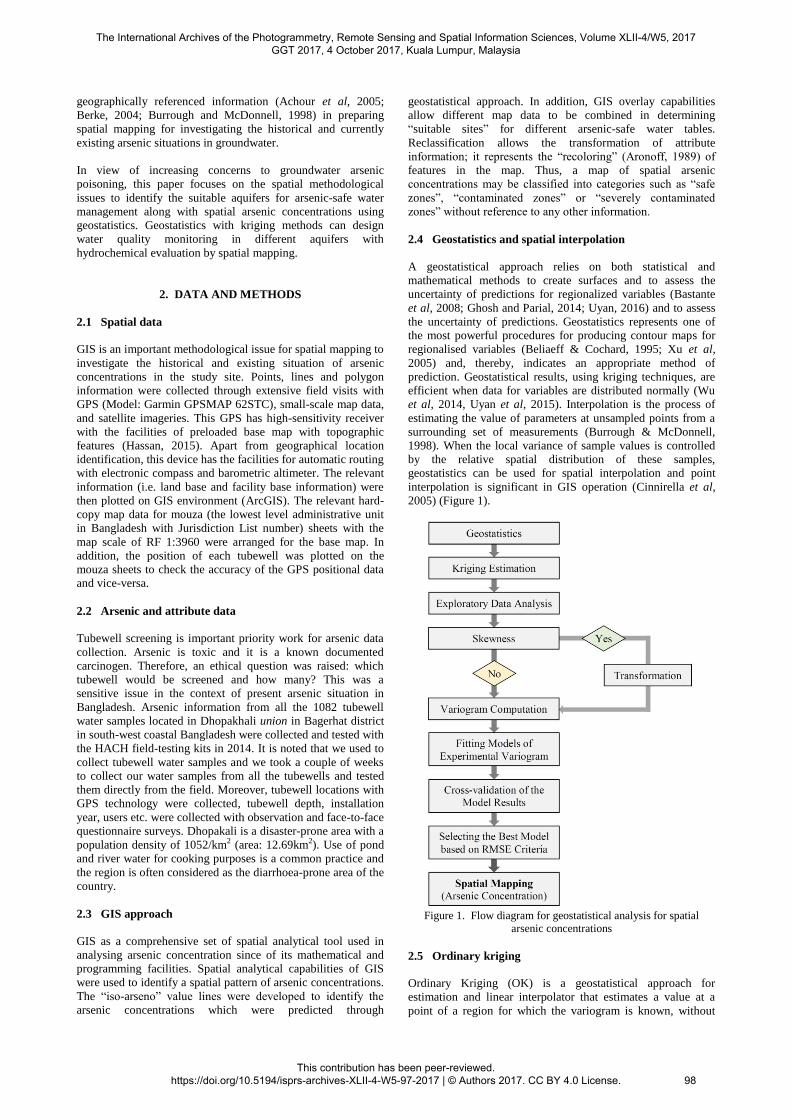
2005) (Figure 1).

Figure 1. Flow diagram for geostatistical analysis for spatial

arsenic concentrations

2.5 Ordinary kriging

Ordinary Kriging (OK) is a geostatistical approach for

estimation and linear interpolator that estimates a value at a

point of a region for which the variogram is known, without


This contribution has been peer-reviewed. https://doi.org/10.5194/isprs-archives-XLII-4-W5-97-2017 | © Authors 2017. CC BY 4.0 License.

98

prior knowledge about the mean of the distribution

(Choudhury, 2015; Dokou et al, 2015). In OK, a random

function model is used, in which the bias and error variance can

both be calculated and then weights are chosen for the nearby

samples such that they ensure that the average error for the

model is zero and the modelled variance is minimized.

The error variance in OK is based on the configuration of the

data and on the variogram, hence is homoscedastic (Yamamoto,

2005). It is not dependent on the data used to make the

estimate. Yamamoto (2005) has also shown that the ordinary

interpolation variance is a better measure of accuracy of the

kriging estimate. OK does not depend on the values of the

samples, which means that the same spatial configuration

always reproduces the same estimation variance in any part of

the area. In order to the estimator to be unbiased in OK, the

sum of these weights needs to equal one (Isaaks and Srivastava,

1989). The estimation equation is a linear weighted

combination of the form (Journel and Huijbregts, 1978):

(1) . . . . . . . . . . . 1ˆ

11

n

iwith

n

ii

i

i

SZSZ 0

OK weights iλ are allocated to the known values in such that

they sum to unity (unbiaseness constraint) and they minimize

the kriging estimation variance (Delbari et al, 2016). The

weights are determined by solving the following system of

equations (Isaaks and Srivastava, 1989):

(2) . . . . .

., . . , ,,

1

1,

1

0

1

n

jj

iji

n

jj

nixxxx

Where, ),γ( ji xx is the average semivariance between pairs of

data locations; μ is the Lagrange parameter for the

minimization of kriging variance; and )γ( , 0xxi is the average

semivariance between the location to be estimated )( 0x and the

thi sample point.

OK can be used for spatial pattern of groundwater arsenic

concentrations since of its high uneven distribution. OK is used

to estimate values when data point values vary or fluctuate

around a constant mean value (Serón et al, 2001). It is applied

for an unbiased estimate of spatial variation of a component.

The estimation variance of OK is used to generate a confidence

interval for the corresponding estimate assuming a normal

distribution of errors (Goovaerts et al, 2005). The unknown

local mean is filtered from the linear estimator by making the

sum of kriging weights to one. OK also provides a measure of

uncertainty attached to each estimated value through

calculating the OK variance (Delbari et al, 2016):

(3) . . . . . . . . . . . . . . ,1

)(00

2

n

i

xxxii

In producing the prediction maps for spatial arsenic

concentrations by the OK method, it was specified the

semivariogram, search neighbourhood, and nugget model in the

interpolation. By using the spherical semivariogram having the

nugget value of 7584.601 and the partial sill of 12882.41, with

200 input neighbours (smoothed neighbours, smoothing factor

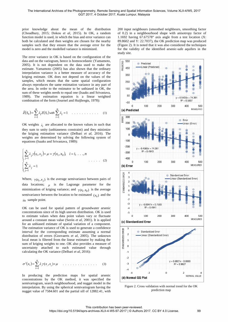
of 0.2) in a neighbourhood shape with anisotropy factor of

1.1692 having 67.67578° axis angle from a test location (X:

89.8602 and Y: 22.7037), the OK prediction map was produced

(Figure 2). It is noted that it was also considered the techniques

for the validity of the identified arsenic-safe aquifers in the

study site.

Figure 2. Cross validation with normal trend for the OK

prediction map



99

2.6 Generalized linear models (GLM)

GLM is a mathematical extension of linear models that do not

force data into unnatural scales, and thereby allow for non-

linearity and non-constant variance structures in the data (Jin et

al, 2005; McCullagh and Nelder, 1989). They are based on an

assumed relationship (link function) between the mean of the

response variable and the linear combination of the explanatory

variables. Since arsenic data are not distributed normally, the

GLM was used for this paper. The Newton-Raphson (maximum

likelihood) optimization technique is used in this study to

estimate the GLM.

Figure 3. Spatial pattern of arsenic concentrations with different

aspects: (a) arsenic in different tubewells; (b) proportion of arsenic

concentrations in each tubewell; and (c) pattern of arsenic

concentrations at ward level

3. RESULTS AND DISCUSSION

3.1 Arsenic concentration

Arsenic concentrations in groundwater can be classified into

different categories based on magnitudes, different permissible

limits, and statistical procedures. The term “contamination” in

this paper refers to the elevated levels of arsenic concentrations

above the Bangladesh Drinking Water Standards (BDWS set by

Department of Environment). On the other hand, the “safe

level” can be categorized into two different classes: one for

WHO permissible limit (10μg/L); and another for the BDWS

(50μg/L). Therefore, arsenic concentrations can be classified

into a number of classes (Table 1 and Figure 3): (a) WHO

permissible level (≤10μg/L); (b) BDWS (10.1-50μg/L); (c)

moderate contamination level (50.1-100μg/L); (d) high

contamination level (100.1-300μg/L); and (e) severe

contamination level (>300μg/L).

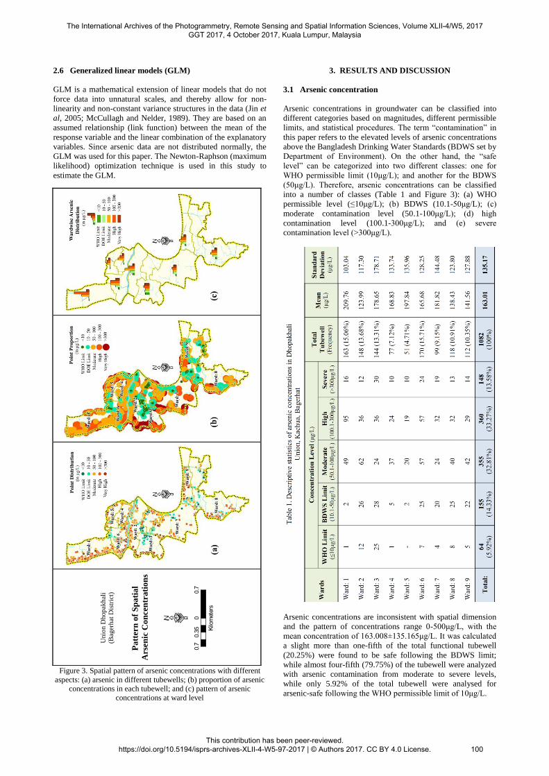
Arsenic concentrations are inconsistent with spatial dimension

and the pattern of concentrations range 0-500μg/L, with the

mean concentration of 163.008±135.165μg/L. It was calculated

a slight more than one-fifth of the total functional tubewell

(20.25%) were found to be safe following the BDWS limit;

while almost four-fifth (79.75%) of the tubewell were analyzed

with arsenic contamination from moderate to severe levels,

while only 5.92% of the total tubewell were analysed for

arsenic-safe following the WHO permissible limit of 10μg/L.

Pa

tter

n o

f S

pa

tia

l

Ars

en

ic C

on

cen

trati

on

s

Unio

n D

hop

akh

ali

(Bag

erh

at D

istr

ict)

·0.

70

0.7

0.35 Ki

lom

eter

s



100

Groundwater arsenic concentrations were found to be different

in each administrative ward in Dhopakhali. Elevated levels of

arsenic were found in all the administrative wards, but highest

mean concentrations were found in Ward 1 (209.76μg/L)

followed by Ward 5 (197.84μg/L), Ward 7 (181.82μg/L), and

Ward 3 (178.65μg/L) (Table 1). On the contrary, the lowest

mean concentration was recorded in Ward 2 (123.99μg/L)

followed by Ward 8 (138.43μg/L), Ward 9 (141.56μg/L), Ward

6 (165.68μg/L) and son on. It is noted that mean arsenic

concentrations in all the administrative wards are much higher

than that of BDWS limit (Table 1 and Figure 3).

There is no deep tubewell (DTW) in Dhopakhali and all the

functional tubewells are within the shallow aquifer with 10-

70m depth. About two-third of the analysed tubewell (704,

65.065%) were installed within 20m depth and they were

analyzed with high arsenic contamination, with mean

concentration of 152.978±130.128μg/L. Moreover, some 378

tubewell were installed in depths more than 20 meters and

mean arsenic concentration were analyzed with

180.648±141.956μg/L.

3.2 Spatial arsenic discontinuity

Which areas are safe and which areas are contaminated? The

answer of this question can be analysed with spatial GIS

analytical capabilities. The OK prediction method shows the

interpolation maps of estimated arsenic concentrations in

Dhopakhali (Figure 4). A point-in-polygon operation through

OK method was performed to analyse spatial arsenic

concentrations. In producing the prediction maps, it was

specified the power function and search neighbourhood in the

interpolation.

Almost one-fifth of the study site are found to be contaminated

with elevated levels of arsenic and they are concentrated all

over the area except in some parts of the southern and middle of

the area. The higher magnitudes are recognizable in the

northwest to southwest parts of the study area (Figure 4a). The

safe areas identified in the OK estimation are especially in

Wards 2 and 3 and the total safe zones cover about 4.17% (53

hectares) of the total study area (Figure 4a). A slight more than

one-fifth (20.24%) of the tubewell (219 out of 1082) conform

to this safe level.

High and severe contamination zones cover about 51.48% (653

hectares) of the study area; while moderate contamination

zones cover about 44.35% (563 hectares). It is noteworthy that

the mean arsenic concentration in Dhopakhali is more than

three times higher (163.01μg/L) than the BDWS (50μg/L) and

more than 16 times higher than the WHO permissible limit

(10μg/L). Moreover, arsenic concentrations were found to be

high erratic with aquifer depth (Figure 4bc).

The pattern of arsenic concentration varies considerably and

unpredictably over distances of a few meters. In the study area,

about 71% of tubewell are located within 43 meters of each

other, but within this distance there are remarkable variations.

The overall pattern of arsenic concentrations in groundwater

within the settlement area in Dhopakhali shows a moderate

contamination running along the banks of the Taleshwar River

to the central part of the area. Safe zones are mainly

concentrated in the central and south-eastern part of the study

area in a scattered manner (Figure 4); while the contaminated

zones are concentrated into the west and north-western parts of

the study area. The contaminated zones are found everywhere

in the study area but with a decrease in the degree of

contamination from west to east. In addition, areas close to

river bank are generally more contaminated; while the south-

eastern parts of the study area are contaminated in a highly

irregular pattern (Figure 4).

(Fil

led

Co

nto

urs)

Pro

ba

bil

ity M

ap

<10

10

- 2

5

25

- 5

0

50

- 1

00

10

0 -

150

15

0 -

200

20

0 -

250

25

0 -

300

30

0 -

400

40

0>

(Ars

en

ic,

µg

/L)

Sp

ati

al A

rse

nic

Dis

co

nti

nu

ity

Unio

n D

hop

akhali

(Bagerh

at

Dis

tric

t)

Leg

en

d ·0.

70

0.7

0.35 Ki

lom

eter

s

Figure 4. Spatial arsenic discontinuity: (a) Overall scenario in the

study site; (b) at the depth less than 24 meters; and (c) at the depth

more than 24 meters

3.3 Safe water demand areas

Which areas will get priority in getting access to safe drinking

water? The answer of this question can detect the safe-water

“command areas” and safe-water “demand areas”. Assurance of

drinking-water safety is a foundation for prevention and control

of waterborne diseases. We have already identified safe and

contaminated areas following the concentration levels of toxic

inorganic arsenic with OK approach. A very small number of

areas were identified as safe zones. The safe water command

areas were identified in Wards 2 and 3 in Dhopakhali and the

total safe zones cover about 12.53% (49 hectares) of acreage

within the settlement area in Dhopakhali.



101

The safe water command areas are located in some parts of the

south-eastern and the middle of Dhopakhali, but very few safe

tubewells are located in irregular pattern in other administrative

Wards (Figure 4). A slightly more than one-fifth (20.24%) of

the tubewells (219 out of 1082) have been identified within the

arsenic-safe zones. It is estimated that people who are living

within the high and severe contamination zones are needed for

safe-water options and the tubewell technology is not suitable

in the contaminated areas. About 87.47% (342 hectares) of the

settlement area are within the unsafe zones. There is no DTW

in Dhopakhali and shallow tubewell (STW) are not suitable in

the identified demand areas. It is noted that installation of more

STW is not required as urgent for safe-water command areas.

3.4 Suitable area for safe tubewell installation

Identification of suitable arsenic-safe aquifer is an important

objective for this study. Suitability analysis is a process of

systematically identifying or rating potential locations with

respect to a particular use. The OK approach has identified the

spatial determination for suitable areas for tubewell installation

with aquifer depths and water-tables (Figure 5).

Arse

nic

-Sa

fe

Gro

un

dw

ate

r S

ou

rce

Leg

end

Un

ion

Dh

op

akh

ali

(Bag

erh

at D

istr

ict)

Set

tlem

ent

area

Su

itab

le a

rea

·0.

70

0.7

0.35 Ki

lom

eter

s

Figure 5. Suitable arsenic-safe aquifer in Dhopakhali

It is noted that only the technological option for both the STW

and DTW was considered for this Spatial Decision-Support

System (SDSS). In considering the safe-water “command

areas” and safe-water “demand areas”, we tried to identify the

suitable areas for installing tubewell in different aquifer depths.

Accordingly, we identified places suitable for installing

tubewell for arsenic-safe water (Figure 5).

Existing arsenic-safe “command areas” in Dhopakhali has been

identified following the safe concentration levels of arsenic in

STW. Apart from STW, people are habituated untreated pond

water for their drinking and cooking purposes in Dhopakhali.

We didn’t consider this water source for safe-water “command

areas” - we have considered only shallow aquifer for suitable

area identification for safe-water through tubewell option.

Figure 5 shows the suitable areas for arsenic-safe water at

shallow aquifer. We have classified the aquifer based on water

table and they were categorized as: (a) lower than 20m depth;

(b) 20-22m depth; and (c) more than 22m depth (Table 3). At

the depth of <20 meters, there are suitable areas for arsenic-safe

STW option for installation more precisely and a number of

settlement clusters in Wards 2, 3, 7, 8, and 9 with sporadic

distribution pattern (Figure 5). At the depth of 22-22 meter,

there is an arsenic-safe water table and it is distributed in all the

administrative Wards except Ward 5 (Figure 5).

It is noted that the identified STW suitable areas are mainly

located in the north-eastern, central, and south-eastern parts of

the study area (Figure 5). Moreover, at the depth of >22 meter,

arsenic-safe water can be tapping mainly from Ward 3, but

there are very small areas for arsenic-safe water and they are in

Wards 1, 2, and 6 (Figure 5 and Table 3). We have identified

from our fieldworks that the sub-surface geology in Dhopakhali

is not suitable for installing DTW. Moreover, the deep aquifer

is heavily concentrated with sodium chloride.

Table 3 shows the arsenic-safe suitable aquifer in the study

area. The areas have been identified at the micro level. People

can easily locate which sites are best fitted for getting arsenic-

safe water at which depth. Moreover, this planning can be

helpful for future strategic plan to provide alternative

technological option in providing safe drinking water.



102

Table 3. Suitable area for arsenic-safe tubewell installation in the

study site

4. CONCLUSIONS

The study has mainly attempt to investigate the spatial pattern

of groundwater arsenic concentrations and to identify suitable

areas for installing STW, the most acceptable water technology.

Mapping the proximity area of arsenic and spatial GIS overlay

capabilities allow different map data to be combined in

determining suitable sites for different arsenic-safe water tables.

Based on the existing arsenic information and characteristics of

water tables, it was demarcated the right areas for arsenic-safe

water at different aquifer depths in the study area. Considering

the situation of groundwater, it can be taken a decision that

further installation of DTW would not be significant for safe

drinking water.

ACKNOWLEDGEMENTS

We would like to express our sincere thanks to the ICCO

Cooperation, Bangladesh for their financial support for a

research project on WASH in Coastal Bangladesh. We are

grateful to Mr Tarit Kanti Biswas and Mr Mahafuzur Rahman

(Biplob) for their support in collecting the relevant arsenic data

from the field. We are grateful to Mr Hussain Ahmad for his

untired support in data entry operation. Finally, we wish to

express our thanks to Mr F M Sarwar Hossain for his

cooperation in completion of the WASH project.

REFERENCES

Achour, M.H, Haroun, A.E, Schult, C.J, Gasem, K.A.M., 2005. A

new method to assess the environmental risk of a chemical process.

Chemical Engineering & Processing, 44(8), pp.901-909.

Antunes, I.M.H.R., Albuquerque, M.T.D., 2013. Using indicator

kriging for the evaluation of arsenic potential contamination in an

abandoned mining area (Portugal). Science of the Total

Environment, 442, pp.545-552.

Aronoff, S., 1989. Geographic Information Systems: a

management perspective. Ottawa, WDL.

Barchowsky, A., States, J.C., 2016. Arsenic-Induced

Cardiovascular Disease. In; States, J.C., (ed), Arsenic: Exposure

Sources, Health Risks, and Mechanisms of Toxicity, John Wiley

and Sons, New Jersey, pp.453-468.

Bastante, F.G., Ordóñez, C., Taboada, J., Matías, J.M., 2008.

Comparison of indicator kriging, conditional indicator simulation

and multiple-point statistics used to model slate deposits.

Engineering Geology, 81, pp.50-59.

Beliaeff, B., Cochard, M.L., 1995. Applying geostatistics to

identification of spatial patterns of fecal contamination in a mussel

farming area (havre de la vanlée, France). Water Research, 29(6),

pp.1541-48.

Berke, O., 2004. Exploratory disease mapping: kriging the spatial

risk function from regional count data. International Journal of

Health Geographics, 3, p.18.

Biswas, A., Neidhardt, H., Kundu, A.K., Halder, D., Chatterjee, D.,

Berner, Z., Jacks, G., Bhattacharya, P., 2014. Spatial, vertical and

temporal variation of arsenic in shallow aquifers of the Bengal

Basin: Controlling geochemical processes. Chemical Geology, 387,

pp.157-169.

Burrough, P.A., McDonnell, R.A., 1998. Principles of

Geographical Information Systems. New York, Oxford University

Press.

Cai, L., Xu, Z., Baoe, P., He, M., Dou, L., Chen, L., Zhou, Y., Zhu,

Y.G., 2015. Multivariate and geostatistical analyses of the spatial

distribution and source of arsenic and heavy metals in the

agricultural soils in Shunde, Southeast China. Journal of

Geochemical Exploration, 148, pp.189-195.

Choudhury, S., 2015. Comparative Study on Linear and Non-

Linear Geostatistical Estimation Methods: A Case Study on Iron

Deposit. Procedia Earth and Planetary Science, 11, pp.131-139.

Cinnirella, S., Buttafuoco, G., Pirrone, N., 2005. Stochastic

analysis to assess the spatial distribution of groundwater nitrate

concentrations in the Po catchment (Italy). Environmental

Pollution, 133(3), pp.569-580.

Clewell, H.J., Gentry, P.R., Yager, J.W., 2016. Considerations for a

Biologically Based Risk Assessment for Arsenic. In States JC (ed),

Arsenic: Exposure Sources, Health Risks, and Mechanisms of

Toxicity, John Wiley and Sons, New Jersey, pp.511-33.

Delbari, M., Amiri, M., Motlagh, M.B., 2016. Assessing

groundwater quality for irrigation using indicator kriging method.

Applied Water Science, 6(4), pp.371-381.

Díaz, S.L., Espósito, M.E., del Carmen Blanco, M., Amiotti, N.M.,

Schmidt, E.S., Sequeira, M.E., Paoloni, J.D., Nicolli, H.B., 2016.

Control factors of the spatial distribution of arsenic and other

associated elements in loess soils and waters of the southern Pampa

(Argentina). Catena, 140, pp.205-216.

Dokou, Z., Kourgialas, N.N., Karatzas, G.P., 2015. Assessing

groundwater quality in Greece based on spatial and temporal

analysis. Environmental Monitoring and Assessment, 187(774),

pp.1-18.

Dummer, T.J.B., Yu, Z.M., Nauta, L., Murimboh, J.D., Parker, L.,

2015. Geostatistical modelling of arsenic in drinking water wells

and related toenail arsenic concentrations across Nova Scotia,

Canada. Science of the Total Environment, 505, pp.1248-1258.

Fee, D.B., 2016. Neurological Effects of Arsenic Exposure. In;

States, J.C., (ed), Arsenic: Exposure Sources, Health Risks, and

Mechanisms of Toxicity, John Wiley and Sons, New Jersey,

pp.193-220.

Flanagan, S.V., Spayd, S.E., Procopio, N.A., Marvinney, R.G.,

Smith, A.E., Chillrud, S.N., Braman, S., Zheng, Y., 2016. Arsenic

in private well water part of 3: Socioeconomic vulnerability to

exposure in Maine and New Jersey. Science of the Total

Environment, 562, pp.1019-1030.

Fraser, B., 2012. Cancer cluster in Chile linked to arsenic

contamination. Lancet, 379(9816), pp.603.

Ghosh, A., Sarkar, D., Dutta, D., Bhattacharyya, P., 2004. Spatial

variability and concentration of arsenic in the groundwater of a

region in Nadia district, West Bengal, India. Archives of Agronomy

and Soil Science, 50, pp.521-527.

Goovaerts, P., AvRuskin, G., Meliker, J., Slotnick, M., Jacquez, G.,

Nriagu, J., 2005. Geostatistical modeling of the spatial variability

of arsenic in groundwater of southeast Michigan. Water Resources

Research, 41, pp..W07013.



103

Hassan, M.M., 2015. Scanning and Mapping the WASH Situation

in Coastal Bangladesh: Problems and Potential. Narrative Report,

Geoecological Research Team (GeRT), Dhaka.

Hassan, M.M., Atkins, P.J., 2011. Application of geostatistics with

Indicator Kriging for analyzing spatial variability of groundwater

arsenic concentrations in southwest Bangladesh. Journal of

Environmental Science and Health, Part A, 46(11), pp.1185-1196.

Hsu, L.I., Wang, Y.H., Chiou, H.Y., Wu, M.M., Yang, T.Y., Chen,

Y.H., Tseng, C.H., Chen, C.J., 2013. The association of diabetes

mellitus with subsequent internal cancers in the arsenic-exposed

area of Taiwan. Journal of Asian Earth Sciences, 73, pp.452-459.

IARC., 2012. A Review of Human Carcinogens: Arsenic, Metals,

Fibres, and Dusts. World Health Organization, International

Agency for Research on Cancer, Lyon (France).

Isaaks, E.H., Srivastava, R.M., 1989. An Introduction to Applied

Geostatistics. New York, Oxford University Press.

Jin, M., Fang, Y., Zhao, L., 2005. Variable selection in generalized

linear models with canonical link functions. Statistics &

Probability Letters, 71, pp.371-382.

Journel, A.G., Huijbregts, C.J., 1978. Mining geostatistics.

Academic Press, San Diego.

Kippler, M., Skröder, H., Rahman, S.M., Tofail, F., Vahter, M.,

2016. Elevated childhood exposure to arsenic despite reduced

drinking water concentrations - A longitudinal cohort study in rural

Bangladesh. Environment International, 86, pp.119-125.

Kuo, C.C., Howard, B.V., Umans, J.G., Gribble, M.O., Best, L.G.,

Francesconi, K.A., Goessler, W., Lee, E., Guallar, E., Navas-Acien,

A., 2015. Arsenic exposure, arsenic metabolism, and incident

diabetes in the strong heart study. Diabetes Care, 38(4), pp.620-

627.

Lin, H.J., Sung, T.I., Chen, C.Y., Guo, H.R., 2013. Arsenic levels

in drinking water and mortality of liver cancer in Taiwan. Journal

of Hazardous Materials, 262, pp.1132-1138.

Liu, C.W., Jang, C.S., Liao, C.M., 2004. Evaluation of arsenic

contamination potential using indicator kriging in the Yun-Lin

Aquifer (Taiwan). Science of the Total Environment, 321, pp.173-

188.

Luczaj, J., Masarik, K., 2015. Groundwater Quantity and Quality

Issues in a Water-Rich Region: Examples from Wisconsin, USA.

Resources, 4(2), pp.323-357.

Ma, L., Wang, L., Jia, Y., Yang, Z., 2016. Arsenic speciation in

locally grown rice grains from Hunan Province, China: Spatial

distribution and potential health risk. Science of the Total

Environment, 557-558, pp.438-444.

McCullagh, P., Nelder, J.A., 1989. Generalized Linear Models.

Chapman and Hall, London.

Medeiros, M.K., Gandolfi, A.J., 2016. Bladder Cancer and Arsenic.

In; States JC (ed), Arsenic: Exposure Sources, Health Risks, and


pp.163-192.

Pardo-Igúzquiza, E., Chica-Olmo, M., Luque-Espinar, J.A.,

Rodríguez-Galiano, V., 2015. Compositional cokriging formapping

the probability risk of groundwater contamination by nitrates.

Science of the Total Environment, 532, pp.162-175.

Peters, S.C., Burkert, L., 2008. The occurrence and geochemistry

of arsenic in groundwaters of the Newark basin of Pennsylvania.

Applied Geochemistry, 23, pp.85-98.

Radloff, K.A., Zheng, Y., Stute, M., Weinman, B., Bostick, B.,

Mihajlov, I., Bounds, M., Rahman, M.M., Huq, M.R., Ahmed,

K.M., Schlosser, P., van Geen, A., 2017. Reversible adsorption and

flushing of arsenic in a shallow, Holocene aquifer of Bangladesh.

Applied Geochemistry, 77, pp.142-157.

Sarma, N., 2016. Skin Manifestations of Chronic Arsenicosis. In;

States, J.C., (ed), Arsenic: Exposure Sources, Health Risks, and


pp.127-136.

Sengupta, S., Sracek, O., Jean, J.S., Lu, H.Y., Wang, C.H., Palcsu,

L., Liu, C.C., Jen, C.H., Bhattacharya, P., 2014. Spatial variation of

groundwater arsenic distribution in the Chianan Plain, SW Taiwan:

Role of local hydrogeological factors and geothermal Sources.

Journal of Hydrology, 518, pp.393-409.

Serón, F.J., Badal, J.I., Sabadell, F.J., 2001. Spatial prediction

procedures for regionalization and 3-D imaging of Earth structures.

Physics of the Earth and Planetary Interiors, 123 (2-4), pp.149-

168.

Sherwood, C.L., Lantz, R.C., 2016. Lung Cancer and Other

Pulmonary Diseases. In; States, J.C., (ed), Arsenic: Exposure

Sources, Health Risks, and Mechanisms of Toxicity, John Wiley

and Sons, New Jersey, pp.137-162.

Smith, A.H., Lingas, E.O., Rahman, M., 2000. Contamination of

drinking-water by arsenic in Bangladesh: a public health

emergency. Bulletin of the World Health Organization, 78(9),

pp.1093-03.

Uyan, M., 2016. Determination of agricultural soil index using

geostatistical analysis and GIS on land consolidation projects: A

case study in Konya/Turkey. Computers and Electronics in

Agriculture, 123, pp.402-409.

Uyan, M., Cay, T., Inceyol, Y., Hakli, H., 2015. Comparison of

designed different land reallocation models in land consolidation: a

case study in Konya/Turkey. Computers and Electronics in

Agriculture, 110, pp.249-258.

WHO., 2015. Drinking Water. Fact Sheet No 391. World Health

Organization. Accessed on May 23, 2016.

[http://www.who.int/mediacentre/factsheets/fs391/en/].

Wilbers, G.J., Becker, M., Nga, L.T., Sebesvari, Z., Renaud, F.G.,

2014. Spatial and temporal variability of surface water pollution in

theMekong Delta, Vietnam. Science of the Total Environment, 485-

486, pp.653-665.

Wu, W., Yin, S., Liu, H., Niu, Y., Bao, Z., 2014. The geostatistic-

based spatial distribution variations of soil salts under long-term

wastewater irrigation. Environmental Monitoring and Assessment,

186(10), pp.6747-6756.

Xu, C., He, H.S., Hu, Y., Chang, Y., Li, X., Bu, R., 2005. Latin

hypercube sampling and geostatistical modeling of spatial

uncertainty in a spatially explicit forest landscape model

simulation. Ecological Modelling, 185(2-4), pp.255-269.

Yamamoto, J. K., 2005. Comparing ordinary kriging interpolation

variance and indicator kriging conditional variance for assessing

uncertainties at unsampled locations. In; Dessureault, S. D.,

Ganguli, R., Kecojevic, V., Dwyer, J. G., (eds), Application of

Computers and Operations Research in the Mineral Industry.

Taylor & Francis, London. Pp.265-269.



104


This contribution has been peer-reviewed. https://doi.org/10.5194/isprs-archives-XLII-4-W5-97-2017 | © Authors 2017. CC BY 4.0 License. 105

Date post:	21-Aug-2019
Category:	Documents
Upload:	dinhcong
View:	219 times
Download:	0 times

ARSENIC-SAFE AQUIFERS IN COASTAL BANGLADESH: AN ... · ARSENIC-SAFE AQUIFERS IN COASTAL BANGLADESH:...

Documents