Metallicity effects on the chromospheric activity–age relation for late-type

dwarfs

H. J. Rocha-Pinto and W. J. MacielInstituto Astronomico e Geofısico, Av. Miguel Stefano 4200, 04301-904 Sao Paulo, Brazil

Accepted 1998 February 21. Received 1998 February 19; in original form 1997 December 23

A B S T R A C T

We show that there is a relationship between the age excess, defined as the difference between

the stellar isochrone and chromospheric ages, and the metallicity as measured by the index

[Fe/H] for late-type dwarfs. The chromospheric age tends to be lower than the isochrone age

for metal-poor stars, and the opposite occurs for metal-rich objects. We suggest that this could

be an effect of neglecting the metallicity dependence of the calibrated chromospheric

emission–age relation. We propose a correction to account for this dependence. We also

investigate the metallicity distributions of these stars, and show that there are distinct trends

according to the chromospheric activity level. Inactive stars have a metallicity distribution

which resembles the metallicity distribution of solar neighbourhood stars, while active stars

appear to be concentrated in an activity strip on the log R0HK × ½Fe=Hÿ diagram. We provide

some explanations for these trends, and show that the chromospheric emission–age relation

probably has different slopes on the two sides of the Vaughan–Preston gap.

Key words: stars: activity – stars: chromospheres – stars: fundamental parameters – stars:

late-type.

1 I N T RO D U C T I O N

The usual method for estimating ages of field stars consists of

comparing the star position, in an MV × log Teff diagram, with

respect to a grid of theoretical isochrones. This procedure is

affected by errors in both coordinates, although the uncertainties

in the determination of the bolometric corrections and effective

temperatures are particularly important.

An alternate method, which seems to be very promising for

estimating ages in late-type dwarfs, makes use of the chromo-

spheric emission (CE) in these stars. From the pioneering work by

Wilson (1963), there is much evidence in the literature that the

stellar chromospheric activity can be associated with the stellar age

(e.g. Skumanich 1972; Barry, Cromwell & Hege 1987; Eggen 1990;

Soderblom, Duncan & Johnson 1991). According to these investi-

gations, young stars show CE levels systematically higher than the

older stars.

Recently, Henry et al. (1996, hereafter HSDB) published the

results of an extensive survey of CE in southern hemisphere G

dwarfs. These data, together with the data previously published by

Soderblom (1985), make possible the study of the CE in a large

number of stars with varying ages and chemical compositions. This

work attempts to discuss the estimate of stellar ages using chromo-

spheric indices in stars with different chemical compositions. In

Section 2, we make a comparison between isochrone and chromo-

spheric ages, and show that the chromospheric ages present system-

atic deviations related to the isochrone ages, as a function of the

metallicity [Fe/H]. In Section 3, we study the differences in the

metallicity distributions of the active and inactive stars, and show that

the active stars seem to be located in a strip in the CE–metallicity

diagram. In Section 4 we give some explanations for this strip and for

other trends in the diagram. Finally, the CE–age relation on both sides

of the Vaughan–Preston gap is treated in Section 5.

2 A C O M PA R I S O N O F I S O C H RO N E A N D

C H RO M O S P H E R I C AG E S

Soderblom et al. (1991) demonstrated that the CE level, as mea-

sured by the index log R0HK, is directly related to the stellar age. This

relation is not a statistical one, but a deterministic relation, the form

of which has not been well determined. Because of the scatter in the

data, Soderblom et al. decided not to choose between a simple

power-law calibration, which would produce many very young

stars, and a more complicated calibration which would preserve the

constancy of the star formation rate.

Also, they argued that the relation between CE and stellar age

seems to be independent of [Fe/H], as the Hyades and Coma

clusters show the same CE levels and have the same age, although

with different chemical compositions. In spite of that, Soderblom et

al. acknowledge that low metallicity stars should have a different

CE–age relation, since in these stars the Ca II H and K lines are

intrinsically shallower than in solar metallicity stars. In this sense,

old metal-poor stars would resemble very young stars due to a

higher log R0HK.

To investigate the metallicity dependence of the chromospheric

activity–age relation, we have used the recent data base by

Mon. Not. R. Astron. Soc. 298, 332–346 (1998)

q 1998 RAS

Edvardsson et al. (1993, hereafter Edv93), which comprises

mainly late F and early G dwarfs. Since the surveys of HSDB

and Soderblom (1985) include mainly G dwarfs, only a fraction of

the stars in the Edv93 sample have measured chromospheric

indices. There are 44 stars in common between these works,

which we will call sample A. For these stars, we have taken

isochrone ages from Edv93 and estimated chromospheric ages

using equation (3) of Soderblom et al. (1991), which can be

written as

log tce ¼ ¹1:50 log R0HK þ 2:25 ð1Þ

where tce is in yr. This is equivalent to R0HK ~ t

¹2=3, and corresponds

The chromospheric activity–age relation 333

q 1998 RAS, MNRAS 298, 332–346

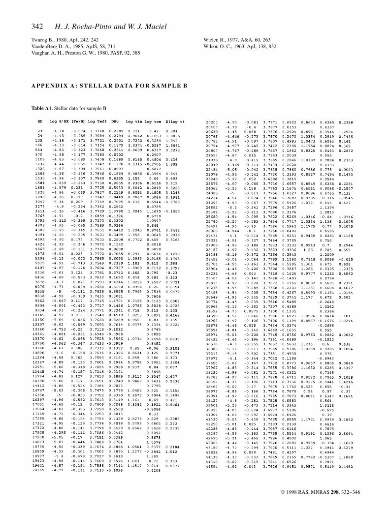
Figure 1. Chromospheric age excesses as a function of [Fe/H]. (a) Sample A (44 stars), using Edv93 ages. (b) Sample A using Ng & Bertelli (1998) ages. (c)

Sample B (471 stars). Symbols are as follows: very active stars (plus signs), active stars (open circles), inactive stars (filled circles), and very inactive stars

(crosses).

to the best power-law fit to their data. It should be noted that the use

of any of the relations suggested by Soderblom et al. (1991) would

produce essentially the same results. In Fig. 1 we show the

difference between the isochrone (tis) and chromospheric (tce)

ages, or age excess, as a function of the metallicity [Fe/H],

Dðlog tÞ ¼ log tis ¹ log tce: ð2Þ

We have used open circles for active stars (log R0HK $ ¹4:75),

and filled circles for inactive stars (log R0HK < ¹4:75, cf. Vaughan &

Preston 1980). Note that, except for a few isolated points, there is a

clear-cut relation between the age excesses and [Fe/H], especially

for the inactive stars, in the sense that the chromospheric ages are

substantially lower than the isochrone ages for metal-poor objects,

while the opposite occurs for metal-rich stars. The age excess is

minimal for metallicities around solar.

Recently, Ng & Bertelli (1998) revised the Edv93 ages, incor-

porating new updated isochrones and absolute magnitudes from

Hipparcos parallaxes. Fig. 1(b) takes into account these revised

ages for the stars in sample A. Note that the scatter is somewhat

lower, and the general trend of Fig. 1(a) is confirmed. The curve in

Figs 1(a) and (b) corresponds to a third-order polynomial fitted to

the inactive stars with ages by Ng & Bertelli (1998).

Aside from sample A, we have built an independent sample with

730 stars (hereafter sample B) by the intersection of the surveys

from HSDB and Soderblom (1985) with the uvby catalogues of

Olsen (1983, 1993, 1994). The metallicity of each star in sample B

was estimated from the calibrations of Schuster & Nissen (1989).

The metallicities for three stars redder than ðb ¹ yÞ ¼ 0:580 were

given by the calibration of Olsen (1984) for K2–M2 stars. In order

to obtain the colours dm1 and dc1, we have adopted the standard

curves ðb ¹ yÞ × m1 and ðb ¹ yÞ × c1 given by Crawford (1975) for

late F and G0 dwarfs, and by Olsen (1984) for mid- and late G

dwarfs. The zero-age main-sequence (ZAMS) curve ðb ¹ yÞ × c1

was corrected as in Edv93 to allow for a dependence on [Fe/H].

Finally, log Teff and DMV (the absolute magnitude deviation above

the ZAMS) were calculated by the calibrations presented by Olsen

(1984). Since all stars in Sample B are expected to be located within

50 pc around the Sun, no correction for reddening was applied to the

photometric indices.

In order to obtain the ages, theoretical isochrones from the work

of VandenBerg (1985) were used. He presents grids of isochrones

for metallicities [Fe/H] = 0.0, ¹0:23, ¹0:46, ¹0:76 and ¹1:00, and

He abundance Y ¼ 0:25. Following the general practice in iso-

chrone age determinations (e.g., Twarog 1980; Soderblom et al.

1991; Edv93), we transformed his isochrones in the plane

MV × log Teff to the plane DMV × log Teff , using tabulated ZAMS

curves given by VandenBerg (1985). Also, we have shifted the

resulting isochrones by d log Teff ¼ ¹0:009 as VandenBerg’s

models seem to be slightly too hot for disc stars, according to

Edv93. We plotted each star from sample B in these five sets of

isochrone grids. An age for the star was estimated by graphic

interpolation in each grid. A first- or second-order polynomial was

fitted to these ages for each star. The stellar age was found by

applying the photometrically calculated [Fe/H] to the polynomial.

We have estimated ages only for the stars which had ages in at least

two sets of grids, amounting to 471 stars.

Table A1 (see Appendix A) shows the 730 stars of sample B. In

the first column we give the HD number. The next columns list,

respectively, log R0HK, [Fe/H], log Teff , DMV , the isochrone loga-

rithmic age, the chromospheric logarithmic age, and the age excess.

The average errors in log Teff and DMV can be estimated from

the calibrations we have used as j log Teff

ÿ �

, 60:011 and

j DMV

ÿ �

, 0:29 mag. These errors imply an age uncertainty of

1.5 to 3 Gyr for the hotter and cooler stars, respectively. An error of

about 0.16 dex in the metallicity calibration further increases the

age uncertainty by about 1 Gyr.

In Fig. 1(c), we show the age excesses for sample B. As well as

the symbols used in the previous panels, we use plus signs for very

active stars (log R0HK > ¹4:20) and crosses for very inactive stars

(log R0HK < ¹5:10). The same general trend arises in this figure:

metal-poor stars show lower chromospheric ages [Dðlog tÞ > 0],

while metal-rich stars show higher chromospheric ages

[Dðlog tÞ < 0]. The curve fitted to sample A is included for compar-

ison. It can be seen that a number of stars deviate from the general

trend, especially active and very active stars, which can also be

observed in Fig. 1(a). On the other hand, almost all the stars which

follow the observed trend between age excess and [Fe/H] have

log R0HK < ¹4:75, and are inactive or very inactive stars. In Fig. 1(b)

the same trend can be observed, although the behaviour of the active

stars is not as clear. In the next section, we will try to understand

why these two classes of stars, which were defined according to the

chromospheric activity level, present different trends regarding

their age excesses.

The data from sample A is more accurate than the data from

sample B, since the photometric calibrations for F and early G

dwarfs are better defined than for late G dwarfs. Moreover, we used

a spectroscopic metallicity in sample A, and a photometric one in

sample B. This is reflected in the higher scatter observed in Fig. 1(c)

as compared with Figs 1(a,b). Note that the scatter observed in Fig. 1

is probably real, as the chromospheric ages depend on the CE index

R0HK which is expected to vary on small time-scales, as a result of the

stellar magnetic cycle. For example, for the Sun a variation in the

range ¹5:10 # log R0HK # ¹4:75 is observed (cf. HSDB). There-

fore, we decided to use sample B only as an independent check of

the results of Figs 1(a,b), and derived a correction to the chromo-

spheric age on the basis of the results shown in Figs 1(a,b). In this

case, the corrected chromospheric age can be written as

log tceðcorrectedÞ ¼ log tce þ Dðlog tÞ ð3Þ

where

Dðlog tÞ ¼ ¹0:193 ¹ 1:382½Fe=Hÿ ¹ 0:213½Fe=Hÿ2þ 0:270½Fe=Hÿ

3;

ð4Þ

which corresponds to the polynomial fit in Fig. 1(b). Note that this

correction should be added to the logarithm of the chromospheric

age, given in yr. This correction can be applied to chromospheric

ages derived from published CE–age calibrations (Soderblom et al.

1991; Donahue 1993, as quoted by HSDB) for log R0HK < ¹4:75 in

the range ¹1:2 < ½Fe=Hÿ < þ0:4.

We checked in the catalogue of Cayrel de Strobel et al. (1997) for

the metallicities of the stars used by Soderblom et al. (1991) for the

building of the CE–age relation. The mean metallicity of these stars

is ¹0:05 dex, with a standard deviation of 0.16 dex. Referring to

Figs 1(a) and (b), we can see that for ½Fe=Hÿ ¼ ¹0:05 we have

Dðlog tÞ . 0, which reinforces our conclusion that the published

CE–age calibrations are valid for solar metallicity stars only.

Another evidence favouring our conclusions is presented in

Fig. 2, where we plot the chromospheric emission index for the

stars of sample A as a function of the calcium abundance [Ca/H]

taken from Edv93. Again, for the inactive stars, the figure shows

that the calcium-rich stars, which are expected to be also metal-rich

and young, have generally lower CE indices. This can be explained

by the fact that these stars have stronger Ca features, which leads to

a lower R0HK and correspondingly higher chromospheric ages, as

334 H. J. Rocha-Pinto and W. J. Maciel

q 1998 RAS, MNRAS 298, 332–346

observed in Fig. 1(a). Inversely, calcium-poor stars show higher

chromospheric indices, which is mainly a result of their weaker Ca

spectral features.

3 M E TA L L I C I T Y D I S T R I B U T I O N S

AC C O R D I N G T O C E L E V E L

Vaughan & Preston (1980) noted that solar neighbourhood stars

could be divided into two populations, namely active and inactive

stars, herafter referred to as AS and IS, respectively. The separation

between these populations is made by the so-called Vaughan–

Preston gap, located around log R0HK ¼ ¹4:75, which is a region of

intermediate activity containing very few stars. Recently, HSDB

showed that the Vaughan–Preston gap is a transition zone instead of

a zone of avoidance of stars. Moreover, they showed that two

additional populations seem to exist: the very active stars

(VAS; log R0HK > ¹4:20) and the very inactive stars (VIS;

log R0HK < ¹5:10Þ.

It is interesting to see whether any trends in the chemical

composition of these four groups exist. At first glance, on the

basis of the existence of a deterministic CE–age relation (Soder-

blom et al. 1991), and of the age–metallicity relation, we would

expect a CE–metallicity relation to exist. The dependence on [Fe/

H] of the CE–age relation, discussed in the previous section, could

hinder or mask such a CE–metallicity relation, and our results could

in principle show whether or not that dependence is real.

Fig. 3 shows the ½Fe=Hÿ × log R0HK diagram for the 730 stars of

sample B. The vertical dashed lines separate the four populations

according to their activity level. Contrary to the argument presented

in the previous paragraph, there seems to be no significant CE–

metallicity relation. Moreover, it is clear that the metallicity

distribution of the four groups are very different from each other.

This is shown more clearly in Fig. 4, where we compare their

metallicity distributions with the solar neighbourhood metallicity

distribution (Rocha-Pinto & Maciel 1996).

It can be seen from Fig. 4 that the metallicity distribution of the IS

is very similar to the solar neighbourhood standard distribution,

suggesting that the IS sample represents the stars in our vicinity

The chromospheric activity–age relation 335

q 1998 RAS, MNRAS 298, 332–346

Figure 2. CE index as a function of the Ca abundances for the stars in Sample A. The values of [Ca/H] are from Edv93. Open circles: active stars; filled circles:

inactive stars.

Figure 3. ½Fe=Hÿ × log R0HK diagram for the 730 stars of sample B. The

vertical dashed lines separate the four populations. The solid lines mark an

apparent ‘activity strip’ where the AS and VAS are mainly located.

very well. This is not surprising, since about 70 per cent of the stars

in the solar neighbourhood are inactive (cf. HSDB). The other

metallicity distributions show some deviations from the standard

distribution, as follows:

(i) The paucity of metal-poor stars in the VIS group is peculiar, as

these should be the oldest stars in the Galaxy, according to their low

CE level, and the oldest stars are supposed to be metal-poor if the

chemical evolution theory is correct.

(ii) The lack of metal-poor stars is even more pronounced in the

AS group, and the transition from the IS to the AS at the Vaughan–

Preston gap suggests an abrupt change in the metallicity distribution

of these stars. The AS have metallicities in a narrow range from

about ¹0:35 dex to +0.15 dex, with an average around ¹0:15 dex. It

is interesting to note that the majority of stars with ½Fe=Hÿ > þ0:20,

which should be very young according to the chemical evolution,

are not AS (young stars according to published CE–age relations),

but appear amongst the VIS and the IS (old stars according to CE

level).

(iii) There are very few VAS, but their metallicities seem to be

lower than the metallicities of the AS. From Fig. 3 it can be seen that

the VAS, together with the AS, appear to be located mainly in a

well-defined ‘activity strip’ on the ½Fe=Hÿ × log R0HK diagram, which

we have marked by solid lines in this figure.

The nature of the VIS and the VAS has already been treated by

HSDB. The VIS are probably stars experiencing a phase similar to

the Maunder Minimum observed in the Sun. The paucity of metal-

poor stars in the VIS group reinforces this conclusion, by ruling out

the hypothesis of old ages for these stars.

The VAS seem to be formed mainly by close binaries. HSDB

have confirmed that many of the VAS in their sample are known to

be RS CVn or W UMa binaries, and have been detected by

ultraviolet and X-ray satellites. In fact, a CE–age relation is not

supposed to be valid for binaries (at least close binaries), since these

stars can keep high CE levels, even at advanced ages, by synchro-

nizing their rotation with the orbital motion (Barrado et al. 1994,

Montes et al. 1996). It is possible that not all VAS are close binaries;

some of them could instead be very young stars. It is significant that

the BY Draconis systems are composed of either close binaries or

very young field stars (Fekel, Moffett & Henry 1986), and that also

the only difference between BY Dra and RS CVn stars is that BY

Dra have later spectral types (Eker 1992). However, taking into

account their metallicity distribution, which shows no stars with

½Fe=Hÿ > ¹0:10 dex, it would appear that the close binaries hypoth-

esis is more appealing, as very young stars should be metal-rich.

Nevertheless, the situation is not so clear. The low [Fe/H] content

of the VAS could be partially responsible for the high log R0HK

indices in these stars, for the reasons explained in Section 2. On the

other hand, it is also known that a high level of chromospheric

activity can decrease the m1 index by filling up the cores of the

metallic lines, simulating a lower [Fe/H] content (Giampapa,

Worden & Gilliam 1979; Basri, Wilcots & Stout 1989). Gimenez

et al. (1991) have shown that the m1 deficiency in active systems

like RS CVn stars is severe and can substantially affect the values of

the photometrically derived stellar parameters. It should be recalled

that even the Sun, which is an inactive star, would look 35 per cent

more metal-poor if observed in a region of activity (Giampapa et al.

1979). Thus, it is very likely that the low metallicity of the VAS is

only an effect of their highly active chromospheres, and not an

indication of older age. A similar conclusion was recently reached

336 H. J. Rocha-Pinto and W. J. Maciel

q 1998 RAS, MNRAS 298, 332–346

Figure 4. Metallicity distributions of the four populations compared to the

solar neighbourhood metallicity distribution from Rocha-Pinto & Maciel

(1996).

Figure 5. The difference between the spectroscopic and photometric metallicity [Fe/H] as a function of the CE level.

by Favata et al. (1997) and Morale et al. (1996) based on photo-

metric and spectroscopic studies of a sample of very active K-type

stars.

4 T H E O R I G I N O F T H E AC T I V I T Y S T R I P

It is now possible to make two hypotheses in order to understand the

activity strip and other trends on the ½Fe=Hÿ × log R0HK diagram.

(a) Stars with lower metallicities should present higher apparent

chromospheric indices log R0HK, since the Ca lines are shallower in

the spectra of metal-poor stars (see Fig. 2). This could produce an

anticorrelation between [Fe/H] and log R0HK.

(b) The chromospheric activity affects the photometric index m1

in such a way that the larger the CE level in a star, the more metal-

poor this star would appear (Gimenez et al. 1991). This can also

produce an anticorrelation as seen in the activity strip beyond the

Vaughan–Preston gap.

The first hypothesis can account well for the deviations between

isochrone and chromospheric ages seen amongst the IS [Figs 1(a)

and (b)]. For the active stars, this is not as obvious, and Fig. 1

suggests that these stars require different corrections, as compared

to the inactive stars. If all active stars were close binaries of RS CVn

or BY Dra types, this could also explain the activity strip. In that

case, close binaries with ½Fe=Hÿ $ þ0:0 would not be found

amongst the VAS, but in the AS group. However, we have found

no preferred region on the ½Fe=Hÿ × log R0HK diagram where the

known resolved binaries (not only close binaries) in our sample B

are located. Moreover, it is well known that many AS stars are not

binaries.

The second hypothesis is particularly suitable for explaining the

The chromospheric activity–age relation 337

q 1998 RAS, MNRAS 298, 332–346

Figure 6. Simulation of the ½Fe=Hÿ × log R0HK diagram for a set of 1750 fictitious stars: (a) age–metallicity relation assuming a constant stellar birthrate; (b) CE–

metallicity diagram assuming no metallicity dependence of the log R0HK index; (c) CE–metallicity diagram adopting equation (4), and correcting the metallicity

of the active stars according to equations (5); (d) the same as panel (c), but the metallicity is corrected using equation (6).

activity strip, since it does not require all active stars to be binaries.

In fact, the shape of the log R0HK × ½Fe=Hÿ diagram, showing a quite

abrupt change in the [Fe/H] distribution at the Vaughan–Preston

gap, suggests that different processes are at work on both sides of

the gap.

To test hypothesis (b), we have searched for spectroscopic

metallicities in Cayrel de Strobel et al. (1997) for the stars in

sample B. For the sake of consistency, we have used the most recent

determination of [Fe/H] for stars having several entries in this

catalogue. Note that the spectroscopic metallicity is not likely to be

affected by the chromospheric activity, and could serve as a tool to

check whether our photometrically derived [Fe/H] abundances are

underestimated.

In Fig. 5, we show the difference D½Fe=Hÿ between the spectro-

scopic and the photometric metallicities as a function of log R0HK. As

in the previous figures, two distinct trends can be seen here. For IS

(log R0HK < ¹4:75), the scatter in D½Fe=Hÿ is high but the stars

appear very well distributed around the expected value

D½Fe=Hÿ < 0. A Gaussian fit to the D½Fe=Hÿ distribution for these

stars gives a mean hDi < 0:03 dex and standard deviation j < 0:13

dex. Such scatter is very likely the result of observational errors as

well as of the inhomogeneity of the spectroscopic data, which was

taken from several sources. For the AS (log R0HK > ¹4:75), the data

clearly show that there is a positive D½Fe=Hÿ, with few deviating

points. According to a Kolmogorov–Smirnov test, the hypothesis

that the D½Fe=Hÿ distributions are the same for both inactive and

active stars can be rejected to a significance level lower than 0.05.

The paucity of points in this part of the diagram makes the

relation between D½Fe=Hÿ and log R0HK somewhat confusing. As a

first aproximation, we will assume that D½Fe=Hÿ is independent of

the CE level, so that it can be written as

D½Fe=Hÿ ¼ 0:17; log R0HK > ¹4:75 ð5aÞ

¼ 0 ; log R0HK # ¹4:75 ð5bÞ

This correction has been applied to the active stars of sample B to

338 H. J. Rocha-Pinto and W. J. Maciel

q 1998 RAS, MNRAS 298, 332–346

Figure 7. (a) Uncorrected and (b) corrected age–metallicity relation for sample B. Also shown are some AMR from the literature.

find the expected metallicity for these stars. The value 0.17 dex

corresponds to the mean D½Fe=Hÿ of the active stars in Fig. 5,

excluding the four stars with negative D½Fe=Hÿ. If these stars are

included, the mean D½Fe=Hÿ decreases down to about 0.11 dex.

From a more physical point of view, it is expected that D½Fe=Hÿ

increases as the CE level increases (Gimenez et al 1991; Favata et

al. 1997). Therefore, we have fitted a straight line by eye again

excluding the deviating stars, and assuming that D½Fe=Hÿ < 0 for

log R0HK # ¹4:75. The obtained expression for this approximation

is

D½Fe=Hÿ ¼ 2:613 þ 0:550 log R0HK; ð6Þ

as can be seen by the straight line in Fig. 5.

To explain the shape of the ½Fe=Hÿ × log R0HK diagram, we have

made a simulation of the diagram in Fig. 3, using a set of 1750

fictitious stars. This set was built in a similar fashion to that

described in Rocha-Pinto & Maciel (1997), using a constant stellar

birthrate and a cosmic scatter in [Fe/H] of 0.20 dex. In Fig. 6(a) we

show the age–metallicity relation for this set of stars. Note that this

figure is shown for illustrative purposes only, and we have made no

attempts to use a relation closer to the real solar neighbourhood

relation. This age–metallicity relation is transformed into a CE–

[Fe/H] relation in Fig. 6(b), using equation (1). This would be the

shape of the ½Fe=Hÿ × log R0HK diagram if a CE–age relation and an

age–metallicity relation exist, and if hypotheses (a) and (b) above

were not valid. It can be seen that Fig. 6(b) does not reproduce the

observed trends of the diagram of Fig. 3. In Fig. 6(c), we show the

same diagram assuming that the ages have an excess Dðlog tÞ

relative to the chromospheric ages, as given in equation (4), and

that the metallicities of the AS and VAS have a deficiency of

D½Fe=Hÿ as given by equations (5). Fig. 6(d) is similar to Fig. 6(c),

except that equation (6) is used instead of equations (5). In Figs

6(b–d), the vertical dashed lines separate the four populations

according to CE level, as in Fig. 3. Fig. 6(c) shows a clear progress

in reproducing Fig. 3 as compared with Fig. 6(b), and Fig. 6(d) can

in fact reproduce fairly well the trends of the observed CE–

metallicity diagram of Fig. 3. Note that all old metal-poor stars in

Fig. 6(b) look more active, that is, younger, in Fig. 6(d). Also, some

young metal-rich stars are shifted to the VIS group in agreement

with the observations. The activity strip beyond the Vaughan–

Preston gap is also very well reproduced in Fig. 6(d). Note that

Fig. 6(c) does not reproduce the activity strip, suggesting that

equation (6) is physically more meaningful than equations (5).

Unfortunately, there are no calibrations for stellar parameters in

chromospherically active stars, which would make it possible to

check whether equation (6) gives the right corrections. However,

the good agreement between our simulations and Fig. 3 suggests

that our procedure to correct the photometric [Fe/H] is reasonably

good.

Another illustration of the correction procedure proposed in this

paper is presented in Fig. 7, where we show the uncorrected age–

metallicity relation (AMR) for sample B (Fig. 7a), as well as the

The chromospheric activity–age relation 339

q 1998 RAS, MNRAS 298, 332–346

Figure 8. dc1 × log R0HK diagram for sample B. The dc1 index can be

regarded as a rough age indicator for our sample.

Table 1. Spatial velocities for VAS and AS in sample B.

HD log R0HK U V W HD log R

0HK U V W HD log R

0HK U V W

166 ¹4.33 ¹15 ¹23 ¹10 61994 ¹4.59 2 ¹23 ¹20 144872 ¹4.74 55 5 5

1835 A ¹4.44 ¹33 ¹13 0 65721 ¹4.67 ¹44 ¹9 ¹26 147513 A ¹4.52 17 ¹3 ¹1

4391 ¹4.55 ¹22 0 7 72905 ¹4.33 10 0 ¹10 150706 ¹4.59 20 ¹4 ¹13

10780 ¹4.61 ¹23 ¹15 ¹4 74576 ¹4.31 ¹26 ¹9 ¹1 152391 ¹4.39 84 ¹108 10

10800 ¹4.60 ¹11 ¹6 ¹10 74842 ¹4.58 27 ¹9 ¹21 160346 ¹4.71 19 ¹1 12

11131 B ¹4.47 20 3 ¹5 82106 ¹4.43 ¹36 ¹13 0 165185 ¹4.43 13 5 ¹9

13445 ¹4.74 ¹109 ¹80 ¹24 88742 ¹4.69 ¹31 ¹44 ¹1 165401 ¹4.65 ¹83 ¹84 ¹38

17051 ¹4.65 ¹27 ¹15 ¹8 88746 A ¹4.70 ¹44 ¹6 ¹1 181321 ¹4.31 ¹13 ¹5 ¹7

17925 ¹4.30 ¹15 ¹16 ¹11 101501 ¹4.50 7 ¹15 ¹4 189087 ¹4.63 ¹34 ¹14 5

20630 ¹4.45 ¹22 ¹4 ¹4 103431 ¹4.68 ¹70 ¹38 ¹12 189931 ¹4.64 ¹44 ¹63 ¹5

20766 ¹4.65 ¹63 ¹42 13 110010 ¹4.47 ¹8 ¹21 ¹13 196850 ¹4.64 ¹1 ¹23 ¹34

22049 ¹4.47 ¹3 8 ¹20 110833 ¹4.72 ¹21 ¹24 13 202628 ¹4.73 ¹11 1 ¹27

25680 ¹4.54 ¹25 ¹15 ¹7 115043 ¹4.43 15 3 ¹8 203244 ¹4.39 1 9 ¹23

30495 ¹4.54 ¹23 ¹9 ¹3 120237 A ¹4.75 ¹49 ¹60 ¹5 205905 ¹4.55 ¹40 ¹15 ¹15

36435 ¹4.44 12 ¹3 ¹19 124580 ¹4.54 11 0 ¹16 206860 ¹4.42 ¹13 ¹20 ¹8

37394 A ¹4.43 ¹12 ¹21 ¹13 128165 ¹4.74 ¹21 7 11 209100 ¹4.56 ¹78 ¹41 3

41700 C ¹4.35 ¹35 ¹11 ¹15 129333 ¹4.23 ¹7 ¹35 ¹3 216803 ¹4.27 ¹6 ¹9 ¹11

42807 ¹4.44 3 ¹25 ¹6 130948 ¹4.45 3 7 ¹6 219709 A ¹4.62 ¹18 ¹40 ¹15

53143 ¹4.52 ¹24 ¹17 ¹15 131582 A ¹4.73 ¹73 ¹71 18 220182 ¹4.41 ¹56 ¹15 ¹2

58830 ¹4.49 5 15 21 131977 ¹4.49 46 ¹21 ¹31 222335 ¹4.73 ¹2 ¹39 6

59967 ¹4.36 ¹11 ¹4 ¹7 134319 ¹4.33 ¹33 ¹15 ¹1

obtained relation after our correction procedure has been applied

(Fig. 7b). Also shown are four average relations from the literature.

It can be seen that the uncorrected sample presents a very large

scatter, so that stars of all metallicities can be found at almost all

ages. On the other hand, the corrected sample shows a much better

agreement with the tendency presented by all previous relations, yet

preserving some scatter averaging 0.2 dex as observed. A full

discussion of this age–metallicity relation will be the subject of a

forthcoming paper.

5 T H E C E – AG E R E L AT I O N F O R AC T I V E

S TA R S

Although a CE–age relation exists amongst late-type dwarfs, its

shape is not well defined. The main uncertainty seems to occur for

stars beyond the Vaughan–Preston gap. Soderblom et al. (1991)

have shown that the slope of the CE–age relation could be steeper

for log R0HK > ¹4:75. This would dramatically affect the interpreta-

tion of the peaks in the chromospheric age distributions as a result of

star formation bursts in our Galaxy (Barry 1988; Noh & Scalo 1990;

Rocha-Pinto & Maciel 1997).

The calibration of the CE–age relation for the active stars, using

Teff and MV derived from photometry, is not as simple as for the

inactive stars, since we do not know very well the extent to which

the photometric indices are affected by the chromospheric activity.

Consider the example shown in Fig. 8. In this plot we show a

dc1 × log R0HK diagram for all stars in sample B. The dc1 index is a

measure of the distance of the star from the ZAMS. In a sample with

a narrow Teff range, as is the case of a sample comprised only of

G dwarfs, it is possible to roughly associate a high dc1 with a greater

age (lower log R0HK), and vice versa. If the AS are really very young

they should have hdc1i & 0:0, and dc1 should become higher as

lower log R0HK values are considered. From Fig. 8, despite the

scatter, we can see a clear relation between dc1 and log R0HK for

the IS and probably also the VIS, as expected on the basis of the

previous discussion. However, the AS group does not show dc1

indices typical of a very young population, and there seems to be no

continuity in the dc1 × log R0HK relation for inactive and active stars.

The plot even suggests that the active stars could be composed of

stars with a variety of ages.

According to Gimenez et al. (1991) and Favata et al. (1997), the

c1 index is less likely to be affected by the chromospheric activity

than the m1 index. However, in the calculation of dc1 we have also

made use of the stellar metallicity, to account for the [Fe/H]

dependence of the ZAMS. This is probably the main reason for

not finding hdc1i , 0:0 for the active stars. If dc1 is incorrect, then

DMV would also be miscalculated, and the isochrone ages found for

these stars would give no information about the real stellar age.

Moreover, the photometric metallicity of the star is needed to

interpolate between the isochrones of different metallicities,

which would be another source of errors. This would produce a

systematic error towards greater ages for the active stars.

In view of these considerations, it is not surprising that most

active stars deviate from the relation between age excess and [Fe/H]

in Figs 1(a) and (c). Note that all single stars with log R0HK > ¹4:75

in fig. 8 from Soderblom et al. (1991) also have isochrone ages

(ranging nearly from 2 to 4 Gyr) systematically greater than their

ages from the calibration, which could be caused by some of these

effects. Until we have photometric calibrations for the stellar

parameters in active stars, we cannot use photometrically derived

temperatures and magnitudes to obtain stellar ages. The best way to

calibrate the CE–age relation beyond the Vaughan–Preston gap

would be to use only open clusters. These objects could have ages

determined by isochrone fitting, a procedure which is not affected

by the CE level of the cluster stars. However, these clusters are

generally distant and their low-mass stars are quite faint to allow CE

measurements (Soderblom et al. 1991). On the other hand, a sample

of stars having Teff and [Fe/H] calculated from their spectra, and MV

from their parallaxes, could have accurate isochrone ages. This is

what happens in Fig. 1(b), where MV is calculated from trigonome-

trical parallaxes. In this figure, the active stars follow more closely

the age excess relation given by equation (4).

A mean age for a group of stars can also be determined on

the basis of its kinematical properties. Soderblom (1990) has

investigated the kinematics of about 30 AS, and has found a

mean age of 1 to 2 Gyr for the group. Nevertheless, he has found

some active stars with kinematics of old population stars. We

decided to reinvestigate the kinematics of the active stars, using a

larger data sample. We have searched for spatial velocities for each

active star of sample B in Gliese & Jahreiß (1991) and Soderblom

340 H. J. Rocha-Pinto and W. J. Maciel

q 1998 RAS, MNRAS 298, 332–346

Figure 9. Spatial motions of 62 active stars listed in Table 1.

(1990). We have also calculated spatial velocities for 17 stars, from

their radial and tangential velocities, proper motions and parallaxes,

obtained from the SIMBAD data base, using the formulae from

Johnson & Soderblom (1987). Table 1 lists 62 active stars with U, V

and W velocities (km s¹1).

Fig. 9 shows the spatial motions of these stars. These panels are

similar to those in Soderblom (1990). However, we have found

several stars with the kinematics of old and intermediate-age

populations. Some of these stars have log R0HK , ¹4:75, and

could be inactive stars. The velocity dispersions jU , jV and jW

are 36, 30 and 14 km s¹1, respectively, which indicates a mean age

of 2 to 4 Gyr for the AS group according to Wielen (1977).

However, an age of 1 to 2 Gyr would be found, in agreement with

Soderblom (1990), if we disregard the stars with large velocities. It

is still early to theorize upon the nature of such high-velocity active

stars, and a larger sample is needed to allow firm conclusions.

We have also found a correlation between jW and log R0HK, which

confirms the existence of a CE–age relation beyond the Vaughan–

Preston gap. That is illustrated in Fig. 10. In this figure, the points

with error bars are the calculated jW for three selected bins of our

sample of active stars, and the triangles show the empirical jW –age

relation according to Wielen (1977). The numbers near the triangles

indicate a mean age for the stellar group with the corresponding jW .

This relation was transformed into a jW –log R0HK relation using the

CE–age calibration by Soderblom et al. (1991). Note that the

velocity dispersions for the active stars are systematically larger

than the dispersions of their presumed coeval stars. This result

suggests that the slope of the CE–age relation for the active stars is

flatter than the slope in equation (3) of Soderblom et al., contrary to

the relation that they propose to preserve the constancy of the star

formation rate. However, this conclusion must be regarded with

caution, as it is not founded on a large data base. In fact, considering

only the open clusters in figure 8 from Soderblom et al., we would

find a steeper slope. Much work is needed to understand the

behaviour of the CE–age relation for active stars.

A program to measure spectroscopically Teff, [Fe/H], and abun-

dance ratios in active stars is currently underway. Together with the

new Hipparcos parallaxes, these data can cast some light on the

discussion of the ages of the AS, and on the shape of the CE–age

relation beyond the Vaughan–Preston gap.

AC K N OW L E D G M E N T S

HJR-P thanks Gustavo F. Porto de Mello for an early suggestion of

the relation between CE and age that has led to this work. We are

indebted to Dr D. Soderblom for some comments on an earlier

version of this paper. This research has made use of the SIMBAD

data base, operated at CDS, Strasbourg, France. This work was

supported by FAPESP and CNPq.

N OT E A D D E D I N P RO O F

After the acceptation of this paper, we learned about a recent

preprint that investigates spectroscopic features of VAS (Soder-

blom, King & Henry 1998). They have found both single and binary

stars amongst the VAS. For some of them it was possible to estimate

[Fe/H]. Two of these stars (HD 37572 and HD 202917) are in our

sample B. The difference D[Fe/H] of them are 0.324 and 0.224,

respectively. These values agree fairly well with our equation (6), at

the activity level of these stars (log R0HK of ¹4:10 and ¹4:06,

respectively).

R E F E R E N C E S

Barrado D., Fernandez-Figueroa M. J., Montesinos B., de Castro E., 1994,

A&A, 290, 137

Barry D. C., 1988, ApJ, 334, 446

Barry D. C., Cromwell R. H., Hege E. K., 1987, ApJ, 315, 264

Basri G., Wilcots E., Stout N., 1989, PASP, 101, 528

Carlberg R. G., Dawson P. C., Hsu T., Vandenberg D. A., 1985, ApJ, 294,

674

Cayrel de Strobel G., Soubiran C., Friel E. D., Ralite N., Francois P., 1997,

A&A, 124, 299

Crawford D. L., 1975, AJ, 80, 955

Donahue R. A., 1993, PhD thesis, New Mexico State Univ.

Edvardsson B., Anderson J., Gustafsson B., Lambert D. L., Nissen P. E.,

Tomkin J., 1993, A&A, 275, 101 (Edv93)

Eggen O. J., 1990, PASP, 102, 166

Eker Z., 1992, ApJS, 79, 481

Favata F., Micela G., Sciortino S., Morale F., 1997, A&A, 324, 998

Fekel F. C., Moffett T. J., Henry G. W., 1986, ApJS, 60, 551

Giampapa M. S., Worden S. P., Gilliam L. B., 1979, ApJ, 229, 1143

Gimenez A., Reglero V., de Castro E., Fernandez-Figueroa M. J., 1991,

A&A, 248, 563

Gliese W., Jahreiß H., 1991, Third Catalogue of Nearby Stars. Astron.

Rechen-Inst. Heidelberg

Henry T. J., Soderblom D. R., Donahue R. A., Baliunas S. L., 1996,

AJ, 111, 439 (HSDB)

Johnson D. R. H., Soderblom D. R., 1987, AJ, 864

Meusinger H., Reimann H.-G., Stecklum B., 1991, A&A, 245, 57

Montes D., Fernandez-Figueroa M. J., Cornide M., de Castro E., 1996, A&A

312, 221

Morale F., Micela G., Favata F., Sciortino S., 1996, A&AS, 119, 403

Ng Y. K., Bertelli G., 1998, A&A, 329, 943

Noh H.-R., Scalo J., 1990, ApJ, 352, 605

Olsen E. H., 1983, A&AS, 54, 55

Olsen E. H., 1984, A&AS, 57, 443

Olsen E. H., 1993, A&AS, 102, 89

Olsen E. H., 1994, A&AS, 104, 429

Rocha-Pinto H. J., Maciel W. J., 1996, MNRAS, 279, 447

Rocha-Pinto H. J., Maciel W. J., 1997, MNRAS, 289, 882

Schuster W. J., Nissen P. E., 1989, A&A, 221, 65

Skumanich A., 1972, ApJ, 171, 565

Soderblom D. R., 1985, AJ, 90, 2103

Soderblom D. R., 1990, AJ, 100, 204

Soderblom D. R., Duncan D. K., Johnson D. R. H., 1991, ApJ, 375, 722

Soderblom D. R., King J. R., Henry T. J., 1998, preprint (astro-ph/9803111)

The chromospheric activity–age relation 341

q 1998 RAS, MNRAS 298, 332–346

Fig. 10. Velocity dispersion jW as a function of log R0HK. The triangles show

the jW –age relation (Wielen 1977), and we have used the CE–age calibra-

tion by Soderblom et al. (1991) to find the log R0HK index for each age.

Twarog B., 1980, ApJ, 242, 242

VandenBerg D. A., 1985, ApJS, 58, 711

Vaughan A. H., Preston G. W., 1980, PASP, 92, 385

Wielen R., 1977, A&A, 60, 263

Wilson O. C., 1963, ApJ, 138, 832

342 H. J. Rocha-Pinto and W. J. Maciel

q 1998 RAS, MNRAS 298, 332–346

A P P E N D I X A : S T E L L A R DATA F O R S A M P L E B

Table A1. Stellar data for sample B.

The chromospheric activity–age relation 343

q 1998 RAS, MNRAS 298, 332–346

Table A1 – continued

344 H. J. Rocha-Pinto and W. J. Maciel

q 1998 RAS, MNRAS 298, 332–346

Table A1 – continued

The chromospheric activity–age relation 345

q 1998 RAS, MNRAS 298, 332–346

Table A1 – continued

346 H. J. Rocha-Pinto and W. J. Maciel

q 1998 RAS, MNRAS 298, 332–346

This paper has been typeset from a TEX=LATEX file prepared by the author.

Table A1 – continued