Remote Sens. 2021, 13, 661. https://doi.org/10.3390/rs13040661 www.mdpi.com/journal/remotesensing

Article

Analysis of Atmospheric and Ionospheric Variations Due

to Impacts of Super Typhoon Mangkhut (1822)

in the Northwest Pacific Ocean

Mohamed Freeshah 1,2,3, Xiaohong Zhang 2,4,5,*, Erman Şentürk 6, Muhammad Arqim Adil 7, B. G. Mousa 1,8,

Aqil Tariq 1, Xiaodong Ren 4,5 and Mervat Refaat 3

1 State Key Laboratory of Information Engineering in Surveying, Mapping and Remote Sensing,

Wuhan University, 129 Luoyu Road, Wuhan 430079, China; mohamedfreeshah@whu.edu.cn (M.F.);

dr.ba haa1@azhar.edu.eg (B.G.M.); aqiltariq@whu.edu.cn (A.T.) 2 Collaborative Innovation Center for Geospatial Technology, 129 Luoyu Road, Wuhan 430079, China;

xhzhang@sgg.whu.edu.cn 3 Department of Surveying Engineering, Faculty of Engineering at Shoubra, Benha University,

108 Shoubra St., Cairo 11629, Egypt; mervat.ameen@feng.bu.edu.eg 4 School of Geodesy and Geomatics, Wuhan University, 129 Luoyu Road, Wuhan 430079, China;

xdren@whu.edu.cn 5 Key Laboratory of Geospace Environment and Geodesy, Ministry of Education, 129 Luoyu Road,

Wuhan 430079, China 6 Department of Surveying Engineering, Kocaeli University, Kocaeli 41001, Turkey;

erman.senturk@kocaeli.edu.tr 7 Department of GNSS, Institute of Space Technology, Islamabad 44000, Pakistan; arqim07@mail.ist.edu.pk 8 Faculty of Engineering, Al‐Azhar University, Cairo 11884, Egypt

* Correspondence: xhzhang@sgg.whu.edu.cn

Abstract: The Northwest Pacific Ocean (NWP) is one of the most vulnerable regions that has been

hit by typhoons. In September 2018, Mangkhut was the 22nd Tropical Cyclone (TC) over the NWP

regions (so, the event was numbered as 1822). In this paper, we investigated the highest amplitude

ionospheric variations, along with the atmospheric anomalies, such as the sea‐level pressure,

Mangkhut’s cloud system, and the meridional and zonal wind during the typhoon. Regional Iono‐

sphere Maps (RIMs) were created through the Hong Kong Continuously Operating Reference Sta‐

tions (HKCORS) and International GNSS Service (IGS) data around the area of Mangkhut typhoon.

RIMs were utilized to analyze the ionospheric Total Electron Content (TEC) response over the max‐

imum wind speed points (maximum spots) under the meticulous observations of the solar‐terres‐

trial environment and geomagnetic storm indices. Ionospheric vertical TEC (VTEC) time sequences

over the maximum spots are detected by three methods: interquartile range method (IQR), en‐

hanced average difference (EAD), and range of ten days (RTD) during the super typhoon

Mangkhut. The research findings indicated significant ionospheric variations over the maximum

spots during this powerful tropical cyclone within a few hours before the extreme wind speed.

Moreover, the ionosphere showed a positive response where the maximum VTEC amplitude vari‐

ations coincided with the cyclone rainbands or typhoon edges rather than the center of the storm.

The sea‐level pressure tends to decrease around the typhoon periphery, and the highest ionospheric

VTEC amplitude was observed when the low‐pressure cell covers the largest area. The possible

mechanism of the ionospheric response is based on strong convective cells that create the gravity

waves over tropical cyclones. Moreover, the critical change state in the meridional wind happened

on the same day of maximum ionospheric variations on the 256th day of the year (DOY 256). This

comprehensive analysis suggests that the meridional winds and their resulting waves may contrib‐

ute in one way or another to upper atmosphere‐ionosphere coupling.

Keywords: atmospheric observations; tropical cyclones; ionospheric disturbances; typhoon

Mangkhut; regional ionosphere maps (RIMs)

Citation: Freeshah, M; Zhang, X;

Şentürk, E; Adil, M.A; Mousa, B.G;

Tariq, A; Ren, X; Refaat, M. Analysis

of atmospheric and Ionospheric

Variations Due to Impacts of Super

Typhoon Mangkhut (1822) in the

Northwest Pacific Ocean.

Remote Sens. 2021, 13, 661.

https://doi.org/10.3390/rs13040661

Academic Editor: Ehsan Foorotan

Received: 3 December 2020

Accepted: 8 February 2021

Published: 11 February 2021

Publisher’s Note: MDPI stays neu‐

tral with regard to jurisdictional

claims in published maps and insti‐

tutional affiliations.

Copyright: © 2021 by the authors.

Licensee MDPI, Basel, Switzerland.

This article is an open access article

distributed under the terms and con‐

ditions of the Creative Commons At‐

tribution (CC BY) license (http://cre‐

ativecommons.org/licenses/by/4.0/).

Remote Sens. 2021, 13, 661 2 of 20

1. Introduction

Principally, geomagnetic storms and solar radiations play a crucial role in the dy‐

namic regime of the ionosphere [1–4]. However, according to the evolution of the atmos‐

phere‐ionosphere coupling theory, the acoustic gravity waves (AGWs) could largely be

associated with some powerful meteorological disturbances that further leads to some

significant ionospheric perturbations [5–7]. Much research has been conducted to distin‐

guish that AGWs could be associated with some powerful meteorological disturbances

[8–10]. In 1960, the theoretical study of atmospheric AGWs have indicated that the iono‐

sphere could respond to severe weather activities for instance lightning, cyclones, torna‐

does, and hurricanes [11]. In addition, a recent paper claimed that large convective cells

(typhoon is a perfect example of such a large‐scale cell), which are the main generator of

electricity in global electric circuit (GEC), lead to the local changes of the ionospheric po‐

tential [12]. Both convective activity and the area covered by electrified clouds are domi‐

nant phenomena for ionospheric potential parameterization.

As it is known, the tropical cyclones (TCs) have powerful vortical structures in such

a way that their origin occupies some near‐equator regions from 5o and 20o in latitudes, in

each hemisphere [13,14]. In Southeastern Asia, TCs are referred to as typhoons whenever

become at the hurricane state [15]. According to the international classification, the stages

of a TC's development could be categorized based on sustained maximum wind speed in

a cyclone: (1) the maximum sustained wind speed under 61 km/h is called tropical depres‐

sion, (2) about 65–115 km/h is called a tropical storm, and, (3) if it gets over 119 km/s, it

will be called as a typhoon in Southeastern Asia and referred to as a hurricane in the At‐

lantic Ocean and the northeastern Pacific Ocean [15–17].

For the first time, Bauer has reported the findings of the ionospheric response to ty‐

phoon passage where the F2 layer's critical frequency, the so‐called foF2, was increased

when the typhoon getting close to the High‐Frequency (HF) Radio station [18]. However,

the foF2 data has low spatial resolution with sparse data on the globe [19,20]. An internal

atmospheric wave (IAWs) could be generated having a period of 1–150 min as a result of

robust tropospheric disturbances from TCs. Under favorable conditions, the IAWs can

pierce into the ionosphere causing ionospheric disturbances [21–23]. Besides, the electric

field and ion oscillation in a studied region would enhance according to the strength of

the cyclone, and this depends on charged aerosols and droplets [24,25]. On the same side,

Sorokin et al. (2005) and Pulinets et al. (2000) reinforced that an ionospheric plasma irreg‐

ularity may be generated by the electric fields over the regions of powerful synoptic per‐

turbations [26,27].

The lower side of the ionosphere is more sensitive to tropospheric activities [22,23],

whereas recording the upper ionospheric (F region) perturbations, caused by the typhoon,

faces several difficulties due to the intensity weakness of the ionospheric response and

large ionospheric vulnerability to geomagnetic effects at those altitudes. However, iono‐

spheric perturbations, associated with the typhoon effect on the upper side of the iono‐

sphere, were mainly revealed by observing the Faraday rotation of the polarization plane

or the Doppler frequency shift [28–31]. According to previous studies, the Doppler sound‐

ing method has false oscillations, where it causes ionospheric disturbances by itself, and

it could be automatically transformed to time series data [32]. So, HF Doppler sounders is

not a very good technique to identify the ionospheric variations induced by cyclones

[30,33].

Recently, the Global Navigation Satellite System (GNSS) provides global coverage

Total Electron Content (TEC) data with high temporal and spatial resolutions [34]. By us‐

ing GNSS observations, the TEC values could be calculated over a ground GNSS station

then the ionospheric response to typhoon could be studied [35]. The highest amplitudes

of slant TEC (STEC) or vertical TEC (VTEC) variations have been recorded during the

cyclone's maximum wind speed (maximum spot) [14]. Many previous studies have been

concentrated more on ionospheric variations associated with TCs on the day of typhoon

landfall and neglected the maximum spot [6,36–38]. On the other side, some researchers

Remote Sens. 2021, 13, 661 3 of 20

focus on the ionospheric response to TCs at evening/night local hours [13,14,38]. Li et al.

(2017) used the VTEC maps from the Center for Orbit Determination in Europe (CODE)

to detect the ionospheric disturbances during the passage of powerful hurricanes and ty‐

phoons in East Asia and North America. However, Global ionosphere maps (GIMs) have

a low spatial resolution of 2.5o in latitude and 5o in longitude [39]; moreover, the VTEC

data depends mainly on the International GNSS Service (IGS) stations and lacks the dense

Continuously Operating Reference Stations (CORS) stations, which makes it have low

spatial resolution, especially for regional case studies. Li et al. (2017) also neglected the

atmospheric parameters, except for satellite cloud photography.

Different mechanisms have been proposed to understand the ionospheric variations

caused by the TCs. Since the typhoons carry rain clouds and thunderstorms, Wilson (1920)

proposed a thunderstorm generator hypothesis by explaining that the thunderstorms de‐

posit negative charges to the Earth and positive charges to the upper atmosphere [40].

Similarly, Rycroft et al. (2012) proposed a GEC model that explains the generation of the

vertical electric field in the atmosphere and the creation of the potential difference be‐

tween Earth's surface and the lower ionosphere due to the thunderstorm and electrified

convective clouds activities [41]. During thunderstorm activity, the ionosphere acquires a

positive potential between 200–500 kV, compared to the Earth’s surface. They further ex‐

plained that this potential difference drives down the vertical conduction current towards

the ground from the ionosphere in all Earth’s fair‐weather regions. The fair‐weather cur‐

rent depends upon the potential difference and the columnar resistance between the

ground and the ionosphere. Furthermore, the horizontal currents flow independently in

the highly conducting ionosphere and the surface of the Earth. The upward flow of the

current towards the ionosphere from the thunderstorm cloud top and from the ground to

the thunderstorm closes the circuit. On the other hand, the propagation and evolution of

the atmospheric AGWs depend upon the propagation medium and its properties [11]. The

altitudinal exponential decrease in the atmospheric pressure generates the upward prop‐

agation of the AGWs. The amplitude of the wave is proportional to the atmospheric den‐

sity, however, the amplitude of the AGWs enhances to maintain the constant energy flux

according to the energy conservation law [11]. At an altitude of ~150 km, the resulting

amplification factor reaches 104, whereas, between 350–400 km, this factor reaches 105‐106.

At these altitudes, the AGWs produces significant perturbation in the ionosphere plasma

through photochemical and dynamical processes.

In this contribution, we produced the regional ionospheric maps with a spatial grid

0.2o in latitude and 0.4o in longitude with 2 h temporal resolution to coincide with CODE

by using dense CORS stations of Hong Kong (HKCORS) in addition to temporal VTEC

from IGS stations around the area of interest. Finally, the atmospheric parameters, such

as sea‐level pressure and the meridional and zonal winds, were retrieved from National

Oceanic and Atmospheric Administration‐Physical Sciences Laboratory (NOAA‐PSL) to

analyze their possible impacts on ionospheric response through the anomaly maps of the

sea level pressure, zonal wind, and meridional wind.

In this paper, we extensively used acronyms throughout the whole text. To make a

proper way to find the corresponding meaning, we listed all used acronyms in alphabeti‐

cal order in Table 1.

Table 1. Lists of acronyms and abbreviations.

Acronyms Corresponding Meaning

AGWs Acoustic Gravity Waves

BL Lower Bound

BU Upper Bound

CCL Carrier‐to‐Code Leveling

CODE Center for Orbit Determination in Europe

CORS Continuously Operating Reference Stations

DOY Day Of the Year

Remote Sens. 2021, 13, 661 4 of 20

Dst Disturbance storm‐time

EAD Enhanced Average Difference

F10.7 solar radio flux at 10.7 cm

GEC Global Electric Circuit

GIMs Global Ionosphere Maps

GNSS Global Navigation Satellite System

HF High‐Frequency

HK Hong Kong

HKT Hong Kong Time

IAWs Internal Atmospheric Waves

IGS International GNSS Service

IPP Ionospheric Pierce Point

IQR InterQuartile Range

Kp the geomagnetic Kp

LOS

MNG

NOAA‐PSL

Line Of Sight

mean of the nearest two grid points

National Oceanic and Atmospheric Administration‐Physical Sciences Laboratory

nT nano Tesla

NWP Northwest Pacific Ocean

R1 lowest range limit

R2 highest range limit

RIMs Regional Ionosphere Maps

RTD Range of ten Days

sfu Solar Flux Unit

SLM single‐layer mapping

STEC Slant Total Electron Content

TC Tropical Cyclone

TEC Total Electron Content

TECU Total Electron Content Unit

VTEC vertical Total Electron Content

2. Data Sources and Analysis Methods

2.1. Space Environment and Super Typhoon Mangkhut Data

According to the recorded data for the maximum sustained wind near the center of

the low‐pressure area of (Mangkhut), there are two points with maximum wind speed at

all as follows in Table 2.

Table 2. The geographical location of the maximum sustained wind speed point in km/h, besides Hong Kong Time (HKT),

date of the year (DOY), and the typhoon classification.

Time (HKT) Days of September

DOY Geographical Location (degree) Classification Maximum sustained wind speed (km/h)

2:00 11 254 14.0 N 142.6 E Severe Typhoon 165

8:00 11 254 14.0 N 141.2 E Super Typhoon 185

14:00 11 254 13.9 N 139.8 E Super Typhoon 205

20:00 11 254 13.7 N 138.6 E Super Typhoon 220

8:00 12 255 13.9 N 136.2 E Super Typhoon 240

2:00 13 256 14.4 N 132.5 E Super Typhoon 240

2:00 14 257 15.2 N 127.9 E Super Typhoon 240

20:00 14 257 17.4 N 124.1 E Super Typhoon 240

23:00 14 257 17.7 N 123.2 E Super Typhoon 250

2:00 15 258 18.0 N 122.3 E Super Typhoon 250

5:00 15 258 18.0 N 121.3 E Super Typhoon 230

11:00 15 258 18.3 N 120.1 E Super Typhoon 195

Remote Sens. 2021, 13, 661 5 of 20

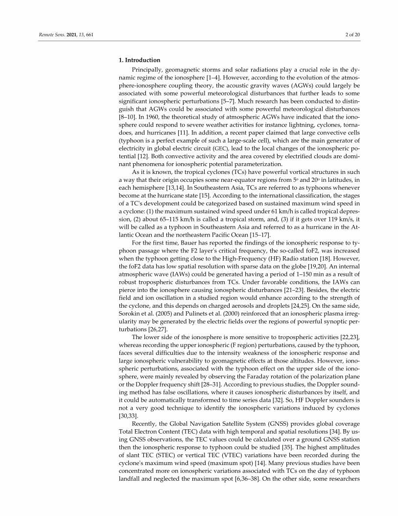
As seen in Table 2 and Figure 1, the maximum wind speed is 250 km/h over the loca‐

tion of (17.7o N, 123.2o E) at 23:00 Hong Kong Time (HKT) on 14 September 2018 and over

the location of (18.0o N, 122.3o E) at 02:00 HKT on 15 September 2018. Previously, Li et al.

(2017) have interpolated the VTEC values of the four grid points nearest to the maximum

spot and apply the method developed by Schaer, (1999) to get the VTEC values [42]. In

this study, we have computed the VTEC time series over the maximum spots as the mean

of the nearest two points, where each point is located on a grid line between two grid

points, and the grid size of the created RIMs is narrower than GIMs which provided high

spatial resolution VTEC data.

Figure 1. Time series of maximum sustained wind speed of Mangkhut from September 14th–17th 2018 with colors repre‐

senting the typhoon classification. (https://www.hko.gov.hk/en/informtc/mangkhut18/maxWind.htm).

2.2. Atmospheric Parameters

The atmospheric parameters were retrieved from NOAA‐PSL via

http://psl.noaa.gov/data/‐composites/day. These data set have a temporal coverage of

daily mean values and spatial coverage of 2.5 x 2.5‐degree global grids (144x73) between

90o N‐90o S latitudes and 0o E‐357.5o E longitudes [43]. The anomaly maps of each observed

day represent differences from the mean value of the previous 5 days. In this study, the

anomaly maps of the sea‐level pressure, zonal and meridional winds for a region between

0‐300 N and 100‐1450 E from September 10–17, 2018 (from DOY 253 to DOY 261), were

used. On the other side, the infrared satellite snapshots of typhoon Mangkhut’s cloud sys‐

tem were selected for certain moments from the Cooperative Institute for Meteorological

Satellite Studies / University of Wisconsin‐Madison via http://tropic.ssec.wisc.edu/ar‐

chive/.

Remote Sens. 2021, 13, 661 6 of 20

2.3. Calculation Process of STEC, VTEC, and RIMs

Many researchers have utilized the data of the GIM assimilative model. Globally, the

data of more than 400 stations are continuously collected to produce GIM pattern, subse‐

quently, generates ionospheric VTEC maps through interpolation and smoothing tech‐

niques which extend from ±87.5 latitudes and ±180 longitudes with spatial resolutions of

2.5 and 5 degrees, respectively [44]. As we can see, produced VTEC maps through GIMs

not only have low spatial resolutions but also depend on limited stations, especially, in

the area of interest around Super Typhoon Mangkhut. Previous studies indicated that the

intensity of tropical typhoons may affect the occurrence rate of ionospheric disturbances

[14]. For that, we collected the GNSS observations from IGS and the HKCORS in the area

around the typhoon. The HKCORS contains 18 CORS evenly set up in Hong Kong for

more details we can refer to (https://www.geodetic.gov.hk/en/satref/satref.htm). There‐

fore, regional ionospheric maps (RIMs) with a high spatial resolution of 0.4 x 0.2 degrees

in longitude and latitude, respectively, have been created through the collected observa‐

tion with a temporal resolution of 2 h to coincide with GIMs. The calculated RIMs cover

110o‐130o E longitudes and 10o‐25o N latitudes. This provides us a very good opportunity

to investigate the ionospheric variations associated with the typhoon Mangkhut by using

high spatial resolution maps.

In this study, the produced RIMs are used to investigate the possible ionospheric

disturbances during the passage of the powerful typhoon Mangkhut over the points of

maximum wind speed [45]. The ionospheric response to the typhoon was analyzed after

computing the ionospheric information. We derived the Slant TEC (STEC) along the line

of sight (LOS) between receivers to GNSS satellites. We can express the ionospheric delay

in length unit and TEC as a function in ƒ frequency (f1 = 1575.42 MHz, f2 = 1227.60 MHz)

[46,47] through the equation:

���� =�׃�

��.������, (1)

where � is the ionospheric delay along a LOS. The GNSS measurements encompass two

L‐band frequencies for the carrier phase and pseudo‐range. The carrier‐to‐code leveling

(CCL) technique is carried out for each continuous arc where the CCL degrades the

pseudo‐range noise, and it eliminates potential ambiguity influence, as well as it retains

the high precision in the carrier‐phase [48]. The CCL method utilizes geometry‐free linear

combinations of code and phase observations to derive the information of the ionosphere

[44,45]. Recently, Zhang et al. (2014) showed that the geometry‐free combination is more

sensitive to ionospheric activity, particularly in the existence of ionospheric scintillation.

The final CCL algorithm form for the processed ionospheric observable can be expressed

through the equation:

���,��� = ��,��� − ���,��� − ��� ��� = ���� + �� + �� + �ε�����

+ ε� , (2)

where ���,��� is the carrier‐phase ionospheric observable leveled to the code‐delay one, and

LI,arc is the carrier‐phase ionospheric observable; Br and BS are the receiver and satellite

hardware delays of the pseudo‐range code, respectively. εL and εp are the noise and multi‐

path for the carrier‐phase ionospheric observations and for the code‐delay measurements,

respectively.

Frequently, TEC is computed by single‐layer mapping (SLM) because the electron

density has a complex spatial distribution [49]. The SLM is used to convert STEC into

VTEC using the mapping function. However, the low elevation angle part is a common

factor that caused errors in different mapping function methods. A lower elevation angle

will cause a larger mapping function error, and higher elevation angle will cause data loss.

In this paper, the elevation cut‐off angle was set to be 15 degrees, which can reduce the

multipath error, on the other hand, can control the mapping error. According to the mod‐

eling‐hypothesis, an SLM where the 2D modeling process assumes that the total free elec‐

trons of the whole ionosphere is concentrated in a thin layer at the elevation with the max

Remote Sens. 2021, 13, 661 7 of 20

electron density [50,51]. The STEC value along the LOS at the Ionospheric Pierce Point

(IPP) can be converted into the corresponding VTEC by using a common ionospheric

mapping function.

���� = cos �arcsin ��

��������� ���� , (3)

where R represents the average radius of the earth, H denotes the altitude of the iono‐

spheric shell layer, and z stands for the satellite zenith angle at the location of the receiver.

We have created a high resolution regional ionospheric maps (RIMs) around the area

of interest, where it can be expressed by the spherical harmonics’ expansion as follows:

����(�, �) = ∑ ∑ ����(����)����

������� (��� cos �� + ��� sin ��), (4)

where s denotes the solar‐fixed longitude, and β represents the geomagnetic latitude of

the IPPs, s = λ ‐ λ0, where λ0 and λ denote the longitude of the sun and the IPP, respectively.

���� = Λ (n, m) ��� represents a normalized associated Legendre polynomial of degree n

and order m; ��� and ��� are spherical harmonic coefficients to be estimated. ��� is the

non‐normalized associated Legendre polynomial, and Λ (n, m) is the normalization con‐

stant can be defined as:

Λ (n, m) = √(� − �)! (2� + 1)(2 − ���)(� + �)!, (5)

(5)

where ��� is the Kronecker delta symbol [34,50]. In this study, we are more concerned about the entire ionospheric disturbance during

the typhoon, rather than a certain layer [49]. The ionospheric single‐shell model with 4th

order and 4th degree for the “Spherical Harmonic” expansion was taken to create the

RIMs for 17 days with 0.4 degrees in longitudes and 0.2 degrees in latitudes. To reduce

the multipath error, the elevation cut‐off angle was set to be 15 degrees. In addition, the

carrier‐phase ambiguity will stay fixed as long as the satellite antenna is not reoriented

(e.g., during the wind‐up); therefore, the term of carrier phase wind‐up has been adjusted

by orbital information and coordinates of each station.

2.4. Methods For Detecting VTEC Disturbances.

In this paper, we proposed a method to compute the VTEC time series values over

maximum wind speed points, so‐called the “maximum spots”, as the mean of the nearest

two grid points (MNG), where the grid size in the created RIMs is relatively small, and

each point of maximum spots located on a grid line.

The VTEC time series over the two maximum spots for 17 days were analyzed by the

interquartile range (IQR) approach. To discover the VTEC variations, the VTEC values of

10 days before September 11, 2018, were used as window length to calculate the upper

quartile, lower quartile, and median, denoted as QU, QL, and M, respectively.

During the process of data analysis, the values of VTECs over the two maximum

spots at the same time were extracted from the RIMs by the proposed MNG method and

ranked from the lowest to the highest in ascending order, i.e., Y1, Y2, . . .Y10. Then, we can

calculate QU, QL, M, and IQR as follows:

�� =(�����)

�, (6)

�� =(�����)

�, (7)

� =(�����)

�, (8)

��� = �� − �� , (9)

By applying the double of IQR as a tolerance (2.7 standard deviations) [52], we can

calculate the upper and lower bounds �� and �� , respectively, as follows:

Remote Sens. 2021, 13, 661 8 of 20

�� = � + 2 ∗ ���, (10)

�� = � − 2 ∗ ���, (11)

Either of the VTECs values falling outside of the corresponding upper or lower

bounds are regarded as abnormal signals. These VTEC anomalies can last for 6 h at least

[33]. According to Hong Kong Observatory, the first and second maximum spots have

coordinates of 17.7o N ‐ 123.2o E and 18.0o N ‐ 122.3o E, respectively. The VTEC time series

over the two maximum spots were computed. Then, the VTEC time series were analyzed

for the next seven days (from DOY 254 to DOY 260) during Super Typhoon Mangkhut

over the two maximum spots.

For a better understanding of how is the data set varied, and try to find key measures

of the detected ionospheric disturbances, a second method was applied, the so‐called

range of ten days (RTD), the VTEC values of the 10 days' data set were ordered to calculate

the range, and then the highest and lowest range limit’s values in the set were compared

with the detected ionospheric disturbances’ DOY.

In order to weaken or eliminate the effects of periodic variations, we applied a third

de‐trending method. In 2020, Freeshah et al. proposed a de‐trending method called one‐

week average (AD) by taking the average of STEC for one week and subtract from STEC

values for the day of the thunderstorm over a mid‐latitude region [53]. We enhanced the

AD approach (EAD) by increasing the number of days for the estimated average value to

be ten days; then, we applied the EAD for VTEC values over the northwest Pacific Ocean

(a low‐latitude region), to detect the ionospheric disturbances over the maximum spots

by using the VTEC time series. In order to avoid the possible geomagnetic effect that—as

a result of the increase of geomagnetic Kp index in these two days—could perturb VTEC

on DOY 254 and DOY 255, we excluded these two DOYs from the average value. In addi‐

tion, in order to make the average value more reliable, we selected a period of ten days,

referred to as the time that preceded the typhoon transformation into the super typhoon

occurred on September 11, 2018. Then, we calculated the average value during these ten

days. In fact, it is reasonable to assume that these ten days can represent the normal state

of the ionosphere in this period.

The EAD method is employed to detect ionospheric disturbances based on an aver‐

age of ten days before the tropical cyclone converted to a super typhoon. The subtraction

of the average simultaneous observations from the next 7 days can lead to an observable

residual. To check the highest VTEC variations among 7 days started from the first day of

the super typhoon, the residual could be calculated from the difference between the ob‐

served value and the estimated (average) value of the ten days, where the highest residual

values could reflect the highest deviation of VTEC. The mathematical process for the EAD

method of de‐trending can be described as follows:

������ = (���������� + ���������� + ⋯ + ����������)/10, (12)

�������� = �������(�) − ������, (13)

where ������ denotes the average VTEC for 10 days, �������� represents the residuals

in VTEC values, and �������(�)indicates a specific day from DOY 254 to DOY 260. The

residuals for 7 days over the maximum spots during typhoon were then compared.

3. Results and Discussion

3.1. Geomagnetic Field and Solar-Terrestrial Environment

Geomagnetic activities and solar radiation are the primary influencers of the iono‐

spheric variations [10]. To distinguish whether the space weather impacts on VTEC devi‐

ations during the typhoon, the solar radio flux at 10.7 cm (F10.7), the Disturbance storm‐

time (Dst), and the geomagnetic Kp indices have been investigated (Figure 2). The geo‐

magnetic field intensity of the earth can be categorized as three levels: low (Dst > ‐50 nT),

Remote Sens. 2021, 13, 661 9 of 20

moderate (‐100 nT < Dst ≤ ‐50 nT), and high (≤‐100 nT), where nT is expressed in nano‐

Tesla [54]. In contrast, solar intensities could be categorized into four intensity levels as

follow: low (F10.7 < 100 sfu), moderate (100 sfu ≤ F10.7 < 150 sfu), high (150 sfu ≤ F10.7 <

200 sfu), and extreme (F10.7 ≥ 200 sfu), where sfu is solar flux unit: 1 sfu = 10⁴ Jy = 10⁻²²

W⋅m⁻²⋅Hz⁻¹ = 10⁻¹⁹ erg⋅s⁻¹⋅cm⁻²⋅Hz⁻¹ [55].

As seen in Figure 2, during the whole period, any evidence of a strong solar activity

or geomagnetic activity is not observed. The lower panel of Figure 2 shows the Dst index

ranging between +20 to ‐20 nT during the typhoon Mangkhut, except for DOY 254 and

DOY 255 (the two excluded days from the IQR window length and the EAD method),

indicating that geomagnetic activity was relatively in steady‐state for the period of data.

As shown in the upper panel, the F10.7 index indicated that the solar activity can be con‐

sidered as low‐level during the typhoon Mangkhut where F10.7 values were less than 100

sfu. There is a low geomagnetic activity (Kp ≤ 4), except on the DOY 257 (Kp ≤ 4.3), DOY

253 (Kp ≤ 5), and the DOY 254 that has the highest value of Kp ≤ 6, indicating a moderate

geomagnetic activity, DOY 254 was excluded from the IQR window length and the EAD

method to skip the possible variation based on moderate geomagnetic activity. Figure 2

indicates that the solar radiation and geomagnetic activity component were relatively sta‐

ble ten days before the typhoon. It is warranted that the ionospheric conditions before the

typhoon, by using the IQR method and EAD de‐trending method, were not affected by

solar and geomagnetic activities, and the results of these methods will be shown later in

Section 3.2.

Figure 2. The F10.7, Kp, and Disturbance storm‐time (Dst) indices in the period from DOY 244 to

DOY 260.

3.2. Ionospheric Variations During Super Typhoon Mangkhut

Figure 3 shows the VTEC time series for 24 h/week over the 1st and 2nd max wind

speed points of the typhoon. The VTEC is expressed by total electron content unit (TECU),

where: 1 TECU = 1016 electrons/m². As shown in Figure 3a, the range of 34.55–1.2 TECU

(highest VTEC and lowest VTEC) was maintained for most of the time during the typhoon

except for DOY 256, where the range increased significantly to become 41.9–4.2 TECU. For

Remote Sens. 2021, 13, 661 10 of 20

DOY 256, VTEC gradually increased to the maximum value of about 08:00 UT (16:00

HKT), and then VTEC gradually decreased. The VTEC anomalous variations can be seen

clearly after 06:00 UT (14:00 HKT). As shown in Figure 3b, the range of 34.6–1.25 TECU

was maintained for most of the time during the typhoon except for DOY 256, where the

range increased significantly to become 42.05–4.35 TECU. For DOY 256, VTEC gradually

increased to the maximum value of about 08:00 UT (16:00 HKT), and then VTEC gradually

decreased. The VTEC anomalous variations can be seen clearly after 06:00 UT (14:00 HKT).

Fig. 3 indicates that the deviation of VTEC values of DOY 256 over the two max wind

speed points could arrive up to more than 7 TECU as a large variation occurred during 7

days.

Figure 3. Vertical Total Electron Content (VTEC) time series over (a) 1st and (b) 2nd maximum spots

of the Super Typhoon Mangkhut, respectively, from September 11–17, 2018 (DOY 254–DOY 260).

According to the Geostationary Operational Environmental Satellite data

(https://hesperia.gsfc.nasa.gov/goes/goes_event_listings/), there is a brief solar flare that

happened during the daytime for three days of the analyzed data (11, 13, and 16 Septem‐

ber 2020); see Table 3.

Table 3. The start, peak, and end time (UTC) of Solar Flares from the Geostationary Operational

Environmental Satellite from September 11–17, 2018 (DOY 254–DOY 260).

Date DOY Start

Time

Peak

Time

End

Time

Class

Sept. 11 DOY 254 7:56 7:59 8:01 B

Sept. 12 DOY 255 NA NA NA NA

Sept. 13 DOY 256 17:56 17:58 18:02 A

Sept. 14 DOY 257 NA NA NA NA

Sept. 15 DOY 258 NA NA NA NA

Sept. 16 DOY 259 4:34 4:35 4:36 A

Sept. 17 DOY 260 NA NA NA NA

To check if there is such an effect on VTEC variations that may be associated with

solar flares, Figure 3 shows that the VTEC of 11 and 16 September is close to the other

days without solar flares, and it has almost the same behavior where the solar flares hap‐

pened for a very short time, 2–6 min, and only for one time a day. In this sense, solar flares

could cause transient ionospheric disturbances by changing electron density, but, once the

action of the solar flare is over, the disturbed plasma tends to the original state [56]. Simi‐

larly, the day of maximum variations on 13 September (DOY 256) also may not be per‐

turbed by solar flares, not only for short time solar flare, but also the time of solar flare

Remote Sens. 2021, 13, 661 11 of 20

that started at 17:56 and continued until 18:02 UTC, after more than 9 h of the maximum

VTEC variations at 08:00 UTC. It is worth indicating that the solar flares class are very

weak (A and/or B classes), and the influences of these flares are not important. So, the

VTEC disturbances on DOY 256 are induced by the typhoon rather than by other random

events.

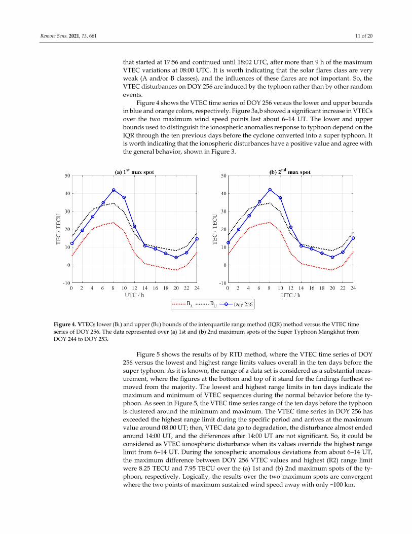
Figure 4 shows the VTEC time series of DOY 256 versus the lower and upper bounds

in blue and orange colors, respectively. Figure 3a,b showed a significant increase in VTECs

over the two maximum wind speed points last about 6–14 UT. The lower and upper

bounds used to distinguish the ionospheric anomalies response to typhoon depend on the

IQR through the ten previous days before the cyclone converted into a super typhoon. It

is worth indicating that the ionospheric disturbances have a positive value and agree with

the general behavior, shown in Figure 3.

Figure 4. VTECs lower (BL) and upper (BU) bounds of the interquartile range method (IQR) method versus the VTEC time

series of DOY 256. The data represented over (a) 1st and (b) 2nd maximum spots of the Super Typhoon Mangkhut from

DOY 244 to DOY 253.

Figure 5 shows the results of by RTD method, where the VTEC time series of DOY

256 versus the lowest and highest range limits values overall in the ten days before the

super typhoon. As it is known, the range of a data set is considered as a substantial meas‐

urement, where the figures at the bottom and top of it stand for the findings furthest re‐

moved from the majority. The lowest and highest range limits in ten days indicate the

maximum and minimum of VTEC sequences during the normal behavior before the ty‐

phoon. As seen in Figure 5, the VTEC time series range of the ten days before the typhoon

is clustered around the minimum and maximum. The VTEC time series in DOY 256 has

exceeded the highest range limit during the specific period and arrives at the maximum

value around 08:00 UT; then, VTEC data go to degradation, the disturbance almost ended

around 14:00 UT, and the differences after 14:00 UT are not significant. So, it could be

considered as VTEC ionospheric disturbance when its values override the highest range

limit from 6–14 UT. During the ionospheric anomalous deviations from about 6–14 UT,

the maximum difference between DOY 256 VTEC values and highest (R2) range limit

were 8.25 TECU and 7.95 TECU over the (a) 1st and (b) 2nd maximum spots of the ty‐

phoon, respectively. Logically, the results over the two maximum spots are convergent

where the two points of maximum sustained wind speed away with only ~100 km.

Remote Sens. 2021, 13, 661 12 of 20

Figure 5. VTECs, lowest (R1) and highest (R2) range limits of range of ten days (RTD) method versus VTEC time series of

DOY 256. The data represented over (a) 1st and (b) 2nd maximum spots of the typhoon from DOY 244 to DOY 253.

Figure 6 indicated the results of the EAD de‐trending technique to detect the VTEC

ionospheric variations during the typhoon over the maximum spots. The differences be‐

tween VTEC values and the average of ten days before the typhoon are depicted below.

As seen, most of the days from DOY 254 to DOY 260 show small residuals that means the

values in the statistical data set are close to the average of the 10 days’ VTEC time series.

Except for DOY 254, there are VTEC variations from around 8–12 UT mainly caused by

the geomagnetic activity where DOY 254 has the highest value of Kp ≤ 6 (Fig. 2). However,

these values are insignificant relatively compared to the VTEC variations on DOY 256.

Fig. 6 shows the significant deviations from ~6‐14 UT where the maximum residual value

was at about 10:00 UT. The large residuals during DOY 256 indicated that the values in

the VTEC time series are farther away from the average value of the specified period of

10 days. According to the previous study, the GNSS‐VTEC GIMs' standard deviations are

about 0.7–4.5 TECU [57]. As it is known that GIMs have a global scale and may not as

accurate as of the derived RIMs [58]. However, we can consider RIMs have the same GIMs

accuracy in the worst case. All days' residuals are within the width of the RIMs accuracy,

except for DOY 256, which has significant deviations. In addition, the large residuals dur‐

ing the peak hours ~6–14 UT of DOY 256 reflect a large amount of variation in VTEC val‐

ues and confirm the results of the previous methods which indicated that the ionospheric

response to super typhoon on DOY 256 during the same period.

Figure 6. VTEC residuals for revealed DOY 256 among a week of the Super Typhoon Mangkhut

from DOY 254 to DOY 260 over (a) 1st and (b) 2nd maximum spots.

Remote Sens. 2021, 13, 661 13 of 20

3.3. Atmospheric Observations During Super Typhoon Mangkhut

To show the effects of the typhoon Mangkhut on the atmospheric climate and try to

enhance the understanding of the troposphere‐ionosphere coupling, the atmospheric pa‐

rameters during the typhoon were retrieved from NOAA‐PSL with 2.5x2.5 degrees spatial

resolution. The anomaly maps of days represent differences from the average value of the

previous 5 days. The maps were obtained from September 10–18, 2018 (DOY 253–DOY

261).

Figure 7 shows that the behavior of the typhoon in the zonal flow’s direction tends

to be weaker and has fast‐moving which causes a relatively slight impact on the local

weather. Meanwhile, Figure 8 shows the meridional flows tend to be stronger with slow‐

moving. This pattern is accountable for most instances of severe weather during the ty‐

phoon. This kind of extreme weather during flow regime is not only marked with strong

storms but also the temperatures can reach their extremes, these weather disturbances can

produce cold waves and heat waves depending on the poleward or equator‐ward direc‐

tion of the flow [59,60]. By returning to Figure 8a–c, we can see the meridional wind has

slight variations from DOY 253–DOY 255. Then, a critical change has happened from DOY

255 (panel c) to DOY 256 (panel d), and this variation indicates a sudden increase in the

meridional wind between the aforementioned DOYs. It is worth indicating that the critical

change of meridional wind happened on the same day of maximum ionospheric varia‐

tions DOY 256. This may be a possible reason that the meridional winds and their result‐

ing waves may contribute to upper atmospheric coupling.

Figure 7. The anomaly maps of zonal wind from September 10–18, 2018; the panels (a)–(i) corresponds to DOY 253–DOY

261, respectively.

Remote Sens. 2021, 13, 661 14 of 20

Figure 8. The anomaly maps of meridional wind on September 10–18, 2018; the panels (a)–(i) corresponds to DOY 253–

DOY 261, respectively.

Figure 9 shows sea‐level pressure from September 10–18, 2018 (DOY 253–DOY 261).

The sea level pressure tends to decrease around the typhoon periphery on DOY 257 (panel

e) and DOY 258 (panel f), and the low‐pressure cell covers the largest area on DOY 256

(panel d). Therefore, the highest ionospheric VTEC disturbance amplitude can be ob‐

served when the low‐pressure cell covers the largest area (Fig. 6 and Fig. 9). Referring to

Table 2, the wind speed in the TC is maximal on DOY 257 with 250 km/h. However, the

highest VTEC disturbance took place on DOY 256 with the second‐highest wind speed of

240 km. The highest VTEC deviations of different periods were observed to increase in

the ionosphere over the peak intensity point of the Mangkhut typhoon. The highest VTEC

variation amplitude was observed on September 13, 2018 (DOY 256), when the sustained

wind speed in the TC had a second‐highest value. And the lowest sea‐level pressure cov‐

ered the maximum area. The highest VTEC variation amplitude could happen before the

max wind speed that may base on the few difference between the highest and second‐

highest wind speed about 10 km/h. In addition, the wind speed of 240 km/h continued for

about 2 days. After that, the storm arrived at the max wind speed of 250 km/h for a short

time of about a few hours. Then, the storm hit Luzon island in the Philippines, and, con‐

sequently, the earth's friction causes the wind to be decreased. This decrease in wind

speed over land is obvious in Figure 1.

Remote Sens. 2021, 13, 661 15 of 20

Figure 9. The anomaly maps of sea‐level pressure on September 10–18, 2018; the panels (a)–(i) corresponds to DOY 253–

DOY 261, respectively.

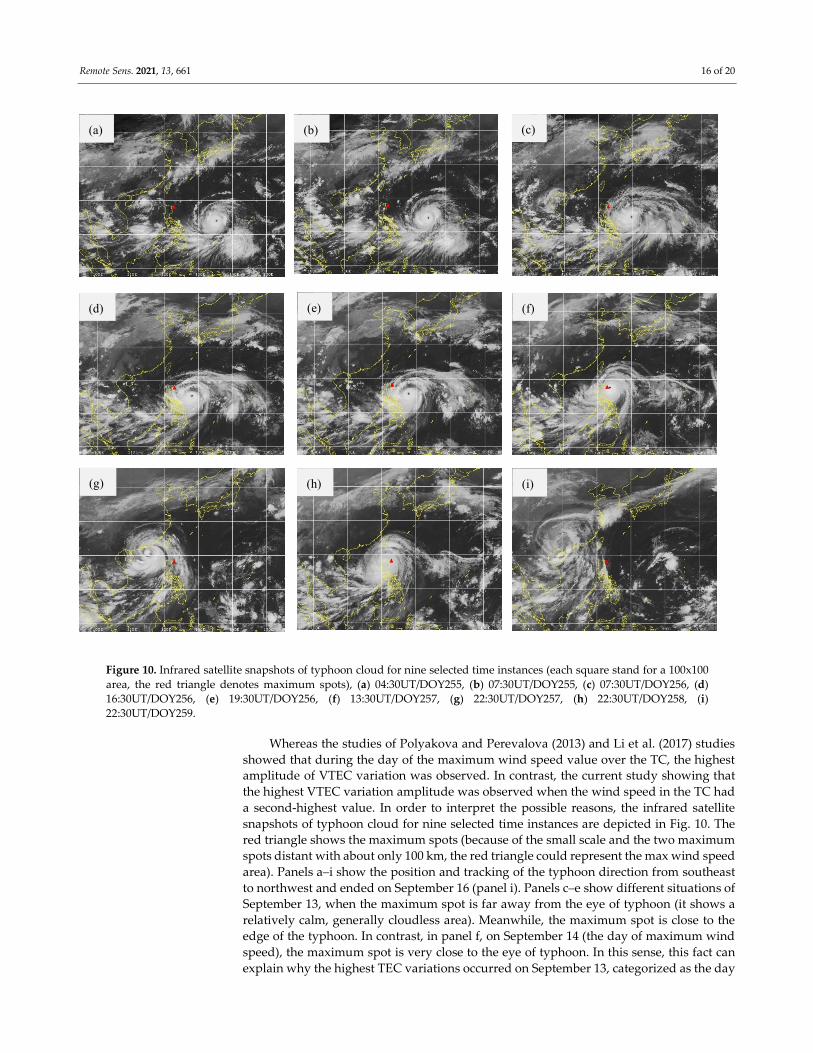
On the other side, the infrared satellite snapshots of typhoon cloud at selected time

instances (Figure 10) shows that the location of the eye storm was close to the point of

maximum speed point. But the previous day the maximum wind speed point was close

to rainbands (typhoon edge), which have a high effect than the storm eye. The typhoon is

a perfect example of large‐scale convective cells, and the electric fields are generated by

thermodynamic convection cells. In this sense, the effects on the ionosphere are stronger,

where a stronger input occurs by electric currents that come from below and can affect the

ionospheric electron‐concentration. It is worth indicating that the typhoon’s eye is cloud‐

less, while the typhoon rainbands display more intense rain that can be associated with

air‐earth currents that are stronger in the rainband areas. Therefore, in the case of the ion‐

ized medium, this fact also justifies the Svensmark effect, which implies that a relevant

percent of precipitation is correlated with cosmic ray flux that influences the Earth's cli‐

mate by means of the production of extra condensation nuclei [61,62].

Remote Sens. 2021, 13, 661 16 of 20

Figure 10. Infrared satellite snapshots of typhoon cloud for nine selected time instances (each square stand for a 100x100

area, the red triangle denotes maximum spots), (a) 04:30UT/DOY255, (b) 07:30UT/DOY255, (c) 07:30UT/DOY256, (d)

16:30UT/DOY256, (e) 19:30UT/DOY256, (f) 13:30UT/DOY257, (g) 22:30UT/DOY257, (h) 22:30UT/DOY258, (i)

22:30UT/DOY259.

Whereas the studies of Polyakova and Perevalova (2013) and Li et al. (2017) studies

showed that during the day of the maximum wind speed value over the TC, the highest

amplitude of VTEC variation was observed. In contrast, the current study showing that

the highest VTEC variation amplitude was observed when the wind speed in the TC had

a second‐highest value. In order to interpret the possible reasons, the infrared satellite

snapshots of typhoon cloud for nine selected time instances are depicted in Fig. 10. The

red triangle shows the maximum spots (because of the small scale and the two maximum

spots distant with about only 100 km, the red triangle could represent the max wind speed

area). Panels a–i show the position and tracking of the typhoon direction from southeast

to northwest and ended on September 16 (panel i). Panels c–e show different situations of

September 13, when the maximum spot is far away from the eye of typhoon (it shows a

relatively calm, generally cloudless area). Meanwhile, the maximum spot is close to the

edge of the typhoon. In contrast, in panel f, on September 14 (the day of maximum wind

speed), the maximum spot is very close to the eye of typhoon. In this sense, this fact can

explain why the highest TEC variations occurred on September 13, categorized as the day

(a) (b) (c)

(d) (e) (f)

(g) (h) (i)

Remote Sens. 2021, 13, 661 17 of 20

of second‐highest wind speed. Subsequently, the distance away/close of the typhoon is a

crucial factor for the control of the magnitude of ionospheric disturbances [38]. Our results

confirm the findings by Li et al. (2017) and Chen et al. (2020) where ionospheric perturba‐

tions in the eye of the storm are fewer than those at the edges of cyclones [63]. It is worth

indicating that the highest VTEC variations have happened with few hours before max

wind speed that may depend on the few difference between the highest and second‐high‐

est wind speed of about 10 km/h, and the second‐highest wind speed of 240 km/h was

continued for about 2 days. Meanwhile, the maximum wind speed was ended within few

hours after the storm arrived at the max wind speed of 250 km/h, the storm hit Luzon

island, Philippines, and the wind speed going speedy decrease based on friction with the

surface of the earth (Fig. 1).

Previous studies verified that the two physical mechanisms for the ionosphere could

respond to powerful typhoons through gravity waves and electric fields [64]. On the same

side, a transient electric field was observed through the sounding rocket and DE‐2 satellite

above Hurricane Debbie, but there is about 10–20 ms the electric field lasted [65]. Thus,

large VTEC deviations values for several hours’ duration, which are observed during

powerful tropical cyclones in the northwest Pacific Ocean, are possibly be the effect of

GEC produced from the thunderstorms [33]. The ionosphere regions E and F could be

triggered through one of both mechanisms: the cyclone produces a low‐pressure vortex

system and generates gravity waves by convection cells [33]. Besides, gravity waves with

vertical wavelengths could arrive at 125–200 km altitudes before going to dissipate [66].

In this regard, the gravity waves could be dissipated in the thermosphere where it could

cool/heats the enclosed fluid and accelerates it in the propagation direction, and the grav‐

ity wave could transfer the energy and momentum to the thermosphere [67,68]. We sug‐

gest that the meridional winds and their resulting cold and heat waves, which depend on

the poleward or equator‐ward direction of the flow, with low‐pressure vortex systems

may contribute as a mechanism to impact the ionosphere over the powerful cyclone.

4. Conclusions

In this study, the ionospheric disturbances observed during powerful typhoon

Mangkhut (1822) in the northwest Pacific Ocean were analyzed using the derived RIMs

which were modeled from HKCORS and IGS stations data for the period before, during,

and after the typhoon and its max wind speed points. The research results indicate that

VTEC's highest variations observed during the second‐highest wind speed with few hours

before max wind speed, and the low‐pressure cell covered the maximum area. These var‐

iations may be a result of the production of the GEC due to the thunderstorm and electri‐

fied convective cloud activities at the rainbands of the typhoon. The vertical conduction

current produced from the GEC flows upward from the thunderstorm cloud to the iono‐

sphere where it endorses severe variations in the electron concentrations. The variation of

space weather indices indicated that the ionospheric conditions were not contributed by

solar and geomagnetic activities. Besides, our research findings confirm the previous re‐

sults by Li et al. (2017) and Chen et al. (2020) in that the ionospheric perturbations in the

eye of the storm are fewer than those at the edges of cyclones. In addition, the critical

change of the meridional wind happened on the same day of maximum ionospheric var‐

iations DOY 256. This may be a possible reason that the meridional winds and their re‐

sulting waves may contribute in one way or another to upper atmospheric coupling. This

study expands evidence for more ionospheric manifestations associated with a powerful

typhoon.

Remote Sens. 2021, 13, 661 18 of 20

Author Contributions: Conceptualization, M.F.; Data curation, M.F., M.R., A.T., and X.R.; Formal

analysis, E.Ş. and M.F.; Funding acquisition, X.Z.; Investigation, M.F. and E.Ş.; Methodology, M.F.;

Project administration, X.Z. and X.R.; Resources, M.F. and M.R.; Software, M.F., E.Ş., M.A.A., and

X.R.; Supervision, X.Z.; Validation, M.F., X.R., and M.R.; Visualization, M.F., E.Ş., M.A.A., B.G.M.,

and M.R.; Writing – original draft, M.F.; Writing – review & editing, M.F., X.Z., E.Ş., M.A.A,

B.G.M, A.T., X.R., and M.R. All authors have read and agreed to the published version of the man‐

uscript.

Funding: This research was funded by the National Science Fund for Distinguished Young Schol‐

ars (no. 41825009), the National Natural Science Foundation of China (no. 41904026), and the Hu‐

bei Provincial Natural Science Foundation of China (no. 2020CFB824).

Institutional Review Board Statement: Not applicable.

Informed Consent Statement: Not applicable.

Data Availability Statement: The data presented in this study are available on request from the

corresponding author.

Acknowledgments: The authors are very grateful to HKCORS and IGS for providing GNSS data,

NASA for providing space weather indices, NOAA‐PSL for providing atmospheric parameters,

cooperative Institute for Meteorological Satellite Studies/the University of Wisconsin‐Madison for

providing infrared satellite snapshots of typhoon cloud. The authors would like to express their

gratitude to Jun Chen, and Nahed Osama for reviewing this manuscript. The authors also would

like to thank the Supercomputing Center of Wuhan University for permitting of use the supercom‐

puting system in numerical calculations. The authors thank for the valuable comments of the re‐

viewers and their promising suggestions to improve this paper.

Conflicts of Interest: The authors declare no conflicts of interest.

References

1. Sojka, J.J.; Raitt, W.J.; Schunk, R.W. Theoretical predictions for ion composition in the high‐latitude winter F‐region for solar

minimum and low magnetic activity. J. Geophys. Res. Space Phys. 1981, 86, 609–621, doi:10.1029/JA086iA04p02206.

2. Hargreaves, J.K. The Solar-Terrestrial Environment; Cambridge University Press; United Kingdom; 1992.

3. Schunk, R.W.; Sojka, J.J. Global ionosphere‐polar wind system during changing magnetic activity. J. Geophys. Res. Space Phys.

1997, 102, 11625–11651, doi:10.1029/97JA00292.

4. Breus, T.K.; Krymskii, A.M.; Crider, D.H.; Ness, N.F.; Hinson, D.; Barashyan, K.K. Effect of the solar radiation in the topside

atmosphere/ionosphere of Mars: Mars Global Surveyor observations. J. Geophys. Res. Space Phys. 2004, 109,

doi:10.1029/2004JA010431.

5. Chane‐ming, F.; Roff, G.; Robert, L.; Leveau, J. Gravity wave characteristics over Tromelin Island during the passage of cyclone

Hudah. Geophys. Res. Lett. 2002, 29, 18‐1–18‐4, doi:10.1029/2001GL013286.

6. Guha, A.; Paul, B.; Chakraborty, M.; De, B.K. Tropical cyclone effects on the equatorial ionosphere: First result from the Indian

sector. J. Geophys. Res. Space Phys. 2016, 121, 5764–5777, doi:10.1002/2016JA022363.

7. Kim, S.; Chun, H.; Baik, J.J. A numerical study of gravity waves induced by convection associated with Typhoon Rusa. Geophys.

Res. Lett. 2005, 32, L24816, doi:10.1029/2005GL024662.

8. Cowling, D.H.; Webb, H.D.; Yeh, K.C. Group rays of internal gravity waves in a wind‐stratified atmosphere. J. Geophys. Res.

1971, 76, 213–220, doi:10.1029/JA076i001p00213.

9. Sorokin, V.M.; Chmyrev, V.M.; Yaschenko, A.K. Electrodynamic model of the lower atmosphere and the ionosphere coupling.

J. Atmos. Sol.-Terr. Phys. 2001, 63, 1681–1691, doi:10.1016/S1364‐6826(01)00047‐5.

10. Afraimovich, E.L.; Voeykov, S.V.; Ishin, A.B.; Perevalova, N.P.; Ruzhin, Y.Y. Variations in the total electron content during the

powerful typhoon of August 5–11, 2006, near the southeastern coast of China. Geomagn. Aeron. 2008, 48, 674–679,

doi:10.1134/s0016793208050113.

11. Hines, C.O. Internal atmospheric gravity waves at ionospheric heights. Can. J. Phys. 1960, 38, 1441–1481.

12. Ilin, N.V.; Slyunyaev, N.N.; Mareev, E.A. Toward a Realistic Representation of Global Electric Circuit Generators in Models of

Atmospheric Dynamics. J. Geophys. Res. Atmos. 2020, 125, doi:10.1029/2019JD032130.

13. Polyakova, A.S.; Perevalova, N.P. Investigation into impact of tropical cyclones on the ionosphere using GPS sounding and

NCEP/NCAR Reanalysis data. Adv. Space Res. 2011, 48, 1196–1210, doi:10.1016/j.asr.2011.06.014.

14. Polyakova, A.S.; Perevalova, N.P. Comparative analysis of TEC disturbances over tropical cyclone zones in the North‐West

Pacific Ocean. Adv. Space Res. 2013, 52, 1416–1426, doi:10.1016/j.asr.2013.07.029.

15. Emanuel, K. Tropical cyclones. Annu. Rev. Earth Planet. Sci. 2003, 31, 75–104, doi:10.1146/annurev.earth.31.100901.141259.

16. Pielke, R.A., Jr.; Pielke, R.A., Sr. Hurricanes: Their Nature and Impacts on Society; John Wiley and Sons: Chichester, NY, USA, 1997.

Remote Sens. 2021, 13, 661 19 of 20

17. Pokrovskaya, I.V.; Sharkov, E.A. Tropical Cyclones and Tropical Disturbances of the World Ocean: Chronology and Evolution, version

3.1 (1983–2005); Poligraph Services: Moscow, Russia, 2006.

18. Bauer, S.J. Correlations between tropospheric and ionospheric parameters. Geofis. Pura E Appl. 1958, 40, 235–240, doi:10.1007/

BF01980131.

19. Zhao, Q.; Yao, Y.; Yao, W. GPS‐based PWV for precipitation forecasting and its application to a typhoon event. J. Atmos. Sol.-

Terr. Phys. 2018, 167, 124–133, doi:10.1016/j.jastp.2017.11.013.

20. Zhao, Y.; Mao, T.; Wang, J.S.; Chen, Z. The 2D features of tropical cyclone Usagi’s effects on the ionospheric total electron

content. Adv. Space Res. 2018, 62, 760–764, doi:10.1016/j.asr.2018.05.02.

21. Hocke, K.; Schlegel, K. A review of atmospheric gravity waves and travelling ionospheric disturbances: 1982–1995. Ann. Geophys.

1996; 14, 917.

22. Kazimirovsky, E.; Herraiz, M.; De la Morena, B.A. Effects on the ionosphere due to phenomena occurring below it. Surv. Geophys.

2003, 24, 139–184, doi:10.1023/A:1023206426746.

23. Laštovička, J. Forcing of the ionosphere by waves from below. J. Atmos. Sol.-Terr. Phys. 2006, 68, 479–497, doi:10.1016/j.ja‐

stp.2005.01.018.

24. Isaev, N.V.; Sorokin, V.M.; Chmyrev, V.M.; Serebryakova, O.N.; Yashchenko, A.K. Disturbance of the Electric Field in the Ion‐

osphere by Sea Storms and Typhoons. Cosm. Res. 2002, 40, 547–553.

25. Isaev, N.V.; Kostin, V.M.; Belyaev, G.G.; Ovcharenko, O.Y.; Trushkina, E.P. Disturbances of the topside ionosphere caused by

typhoons. Geomagn. Aeron. 2010, 50, 243–255, doi:10.1134/S001679321002012X.

26. Sorokin, V.M.; Isaev, N.V.; Yaschenko, A.K.; Chmyrev, V.M.; Hayakawa, M. Strong DC electric field formation in the low lati‐

tude ionosphere over typhoons. J. Atmos. Sol.-Terr. Phys. 2005, 67, 1269–1279, doi:10.1016/j.jastp.2005.06.014.

27. Pulinets, S.A.; Boyarchuk, K.A.; Hegai, V.V.; Kim, V.P.; Lomonosov, A.M. Quasielectrostatic model of atmosphere‐thermo‐

sphere‐ionosphere coupling. Adv. Space Res. 2000, 26, 1209–1218, doi:10.1016/S0273‐1177(99)01223‐5.

28. Bertin, F.; Testud, J.; Kersley, L. Medium scale gravity waves in the ionospheric F‐region and their possible origin in weather

disturbances. Planet. Space Sci. 1975, 23, 493–507, doi:10.1016/0032‐0633(75)90120‐8.

29. Hung, R.J.; Kuo, J. Ionospheric observation of gravity waves associated with Hurricane Eloise. J. Geophys. 1978, 45, 67–80.

30. Huang, Y.; Cheng, K.; Chen, S. On the detection of acoustic‐gravity waves generated by typhoon by use of real time HF Doppler

frequency shift sounding system. Radio Sci. 1985, 20, 897–906, doi:10.1029/RS020i004p00897.

31. Xiao, Z.; Xiao, S.G.; Hao, Y.Q.; Zhang, D.H. Morphological features of ionospheric response to typhoon. J. Geophys. Res. Space

Phys. 2007, 112, doi:10.1029/2006JA011671.

32. Chum, J.; Liu, J.; Podolsk, K.; Sindel, T. Infrasound in the ionosphere from earthquakes and typhoons. J. Atmos. Sol.-Terr. Phys.

2018, 171, 72–82, doi:10.1016/j.jastp.2017.07.022.

33. Li, W.; Yue, J.; Yang, Y.; Li, Z.; Guo, J.; Pan, Y.; Zhang, K. Analysis of ionospheric disturbances associated with powerful cyclones

in East Asia and North America. J. Atmos. Sol.-Terr. Phys. 2017, 161, 43–54, doi:10.1016/j.jastp.2017.06.012.

34. Ren, X.; Zhang, X.; Xie, W.; Zhang, K.; Yuan, Y.; Li, X. Global Ionospheric Modelling using Multi‐GNSS: BeiDou, Galileo,

GLONASS and GPS. Sci. Rep. 2016, 6, doi:10.1038/srep33499.

35. Yang, Z.; Liu, Z. Observational study of ionospheric irregularities and GPS scintillations associated with the 2012 tropical cy‐

clone Tembin passing Hong Kong. J. Geophys. Res. Space Phys. 2016, 121, 4705–4717, doi:10.1002/2016JA022398.

36. Song, Q.; Ding, F.; Zhang, X.; Mao, T. GPS detection of the ionospheric disturbances over China due to impacts of Typhoons

Rammasum and Matmo. J. Geophys. Res. Space Phys. 2017, 122, 1055–1063, doi:10.1002/2016JA023449.

37. Song, Q.; Ding, F.; Zhang, X.; Liu, H.; Mao, T.; Zhao, X.; Wang, Y. Medium‐Scale Traveling Ionospheric Disturbances Induced

by Typhoon Chan‐hom Over China. J. Geophys. Res. Space Phys. 2019, 124, 2223–2237, doi:10.1029/2018JA026152.

38. Chen, J.; Zhang, X.; Ren, X.; Zhang, J.; Freeshah, M.; Zhao, Z. Ionospheric disturbances detected during a typhoon based on

GNSS phase observations: A case study for typhoon Mangkhut over Hong Kong. Adv. Space Res. 2020, 66, 1743–1753,

doi:10.1016/j.asr.2020.06.006.

39. Ren, X.; Chen, J.; Li, X.; Zhang, X.; Freeshah, M. Performance evaluation of real‐time global ionospheric maps provided by

different IGS analysis centers. GPS Solut. 2019, 23, doi:10.1007/s10291‐019‐0904‐5.

40. Wilson, C.T.R. Investigation on lightning discharges and on the electric field of thunderstorms. Philos. Trans. R. Soc. Lond. 1920,

A221, 73–115, doi:10.1098/rsta.1921.0003.

41. Rycroft, M.J.; Nicoll, K.A.; Aplin, K.L.; Harrison, R.G. Recent advances in global electric circuit coupling between the space

environment and the troposphere. J. Atmos. Sol.-Terr. Phys. 2012, 90–91, 198–211, doi:10.1016/j.jastp.2012.03.015.

42. Schaer, S. Mapping and Predicting the Earth’s Ionosphere Using the Global Positioning System; University Bern: Bern, Switzerland,

1999.

43. Kalnay, E.; Kanamitsu, M.; Kistler, R.; Collins, W.; Deaven, D.; Gandin, L.; Zhu, Y. The NCEP/NCAR 40‐year reanalysis project.

Bull. Am. Meteorol. Soc. 1996, 77, 437–472, doi:10.1175/1520‐0477(1996)077<0437:TNYRP>2.0.CO;2.

44. Alizadeh, M.M.; Schuh, H.; Todorova, S.; Schmidt, M. Global ionosphere maps of VTEC from GNSS, satellite altimetry, and

Formosat‐3/COSMIC data. J. Geod. 2011, 85, 975–987.

45. Shi, K.; Liu, X.; Guo, J.; Liu, L.; You, X.; Wang, F. Pre‐Earthquake and coseismic Ionosphere disturbances of the Mw 6.6 Lushan

Earthquake on 20 April 2013 Monitored by CMONOC. Atmosphere 2019, 10, 216, doi:10.3390/ATMOS10040216.

46. Hofmann‐Wellenhof, B.; Lichtenegger, H.; Collins, J. Global Positioning System Theory and Practice, 1st ed.; Springer; Wien New

York, USA: 1992; ISBN 978‐3‐7091‐5126‐6.

Remote Sens. 2021, 13, 661 20 of 20

47. Ren, X.; Chen, J.; Li, X.; Zhang, X. Ionospheric total electron content estimation using GNSS carrier phase observations based

on zero‐difference integer ambiguity: Methodology and assessment. IEEE Trans. Geosci. Remote Sens. 2020,

doi:10.1109/tgrs.2020.2989131.

48. Li, Z.; Yuan, Y.; Fan, L.; Huo, X.; Hsu, H. Determination of the Differential Code Bias for Current BDS Satellites. IEEE Trans.

Geosci. Remote Sens. 2013, 52, 3968–3979, doi:10.1109/TGRS.2013.2278545.

49. Nina, A.; Nico, G.; Odalovic, O.; Cadez, V.M.; Todorovic Drakul, M.; Radovanovic, M.; Popovic, L.C. GNSS and SAR Signal

Delay in Perturbed Ionospheric D‐Region during Solar X‐Ray Flares. IEEE Geosci. Remote Sens. Lett. 2020, 17, 1198–1202,

doi:10.1109/LGRS.2019.2941643.

50. Sidorenko, K.A.; Vasenina, A.A. Ionospheric parameters estimation using GLONASS / GPS data. Adv. Space Res. 2016, 57, 1881–

1888, doi:10.1016/j.asr.2016.01.025.

51. Zhang, W.; Zhao, X.; Jin, S.; Li, J. Ionospheric disturbances following the March 2015 geomagnetic storm from GPS observations

in China. Geod. Geodyn. 2018, 9, 288–295, doi:10.1016/j.geog.2018.02.001.

52. Li, W.; Guo, J.; Yue, J.; Yang, Y.; Li, Z.; Lu, D. Contrastive research of ionospheric precursor anomalies between Calbuco volcanic

eruption on April 23 and Nepal earthquake on April 25, 2015. Adv. Space Res. 2016, 57, 2141–2153, doi:10.1016/j.asr.2016.02.014.

53. Freeshah, M.; Zhang, X.; Chen, J.; Zhao, Z.; Osama, N.; Sadek, M.; Twumasi, N. Detecting Ionospheric TEC Disturbances by

Three Methods of Detrending through Dense CORS During A Strong Thunderstorm. Ann. Geophys. 2020, 63, 667, doi:10.4401/ag‐

8372.

54. Chen, H.‐F. Analysis of the diurnal and semiannual variations of Dst index at different activity levels. J. Geophys. Res. Space Phys.

2004, 109, doi:10.1029/2003JA009981.

55. Lennartsson, W. Energetic (0.1‐to 16‐keV/e) magnetospheric ion composition at different levels of solar F10.7. J. Geophys. Res.

Space Phys. 1989, 94, 3600–3610.

56. Nina, A.; Čadež, V.M. Electron production by solar Ly‐α line radiation in the ionospheric D.‐region. Adv. Space Res., 2014, 54,

1276–1284, doi:10.1016/j.asr.2013.12.042.

57. Chen, P.; Liu, H.; Ma, Y.; Zheng, N. Accuracy and consistency of different global ionospheric maps released by IGS ionosphere

associate analysis centers. Adv. Space Res. 2020, 65, 163–174, doi:10.1016/j.asr.2019.09.042.

58. Li, B.; Wang, M.; Wang, Y.; Guo, H. Model assessment of GNSS‐based regional TEC modeling: Polynomial, trigonometric series,

spherical harmonic and multi‐surface function. Acta Geod. Geophys. 2019, 54, 333–357, doi:10.1007/s40328‐019‐00262‐8.

59. GILL, A.E. Chapter Thirteen—Instabilities, Fronts, and the General Circulation. In Atmosphere—Ocean Dynamics; Elsevier, Cal‐

ifornia, USA: 1982; pp. 549–593.

60. Hartmann, D.L. Chapter 6—Atmospheric General Circulation and Climate. In Global Physical Climatology, 2nd ed.; Elsevier,

Amsterdam, Netherlands: 2016; pp. 159–193.

61. Quinn, J.M. Mapping the global lithosphere: Of mega‐diameter meteorite impact sites within the global lithosphere. In Solar-

Terrestrial Environmental Research Institute (STERI); Lakewood, CO, USA, 2012; p. 154.

62. Quinn, J.M. Global remote sensing of Earth’s magnetized lithosphere. In Solar-Terrestrial Environmental Research Institute (STERI);

Lakewood, CO, USA, 2014; p. 253.

63. Freeshah, M.; Zhang, X.; Ren, X. Using Interquartile Range to Detect TEC Perturbations Associated with A Tropical Cyclone

Crossing through The South China Sea. In Proceedings of the Intercontinental Geoinformation Days (IGD), Mersin, Turkey, 25–

26 November 2020; pp. 28–31.

64. Bishop, R.L.; Aponte, N.; Earle, G.D.; Sulzer, M.; Larsen, M.F.; Peng, G.S. Arecibo observations of ionospheric perturbations

associated with the passage of Tropical Storm Odette. J. Geophys. Res. Space Phys. 2006, 111, doi:10.1029/2006JA011668.

65. Kelley, M.C.; Siefring, C.L.; Pfaff, R.F.; Kintner, P.M.; Larsen, M.; Green, R.; Holzworth, R.H.; Hale, L.C.; Mitchell, J.D.; Vine,

D.L. Electrical measurements in the atmosphere and the ionosphere over an active thunderstorm: 1. Campaign overview and

initial ionospheric results. J. Geophys. Res. 1985, 90, 9815–9823.

66. Vadas, S.L.; Fritts, D.C. Influence of solar variability on gravity wave structure and dissipation in the thermosphere from trop‐

ospheric convection. J. Geophys. Res. Space Phys. 2006, 111, doi:10.1029/2005JA011510.

67. Vadas, S.L. Compressible f‐plane solutions to body forces, heatings, and coolings, and application to the primary and secondary

gravity waves generated by a deep convective plume. J. Geophys. Res. Space Phys. 2013, 118, 2377–2397, doi:10.1002/jgra.50163.

68. Vadas, S.L., Makela, J.J., Nicolls, M.J.; Milliff, R.F. Excitation of gravity waves by ocean surface wavepackets Upward propaga‐

tion and reconstruction of the thermospheric gravity wave field. J. Geophys. Res. Space Phys. 2015, 120, 9748–9780,

doi:10.1002/2015JA021430.