Article

Effect of family labour on output of farmsin selected EU Member States: A non-parametric quantile regression approach

Kostov, Phillip, Davidova, Sophia and Bailey, Alastair

Available at http://clok.uclan.ac.uk/21022/

Kostov, Phillip ORCID: 0000-0002-4899-3908, Davidova, Sophia and Bailey, Alastair (2018) Effect of family labour on output of farms in selected EU Member States: A non-parametric quantile regression approach. European Review of Agricultural Economics, 45 (3). pp. 367-395. ISSN 0165-1587

It is advisable to refer to the publisher’s version if you intend to cite from the work.http://dx.doi.org/10.1093/erae/jbx036

For more information about UCLan’s research in this area go to http://www.uclan.ac.uk/researchgroups/ and search for <name of research Group>.

For information about Research generally at UCLan please go to http://www.uclan.ac.uk/research/

All outputs in CLoK are protected by Intellectual Property Rights law, includingCopyright law. Copyright, IPR and Moral Rights for the works on this site are retainedby the individual authors and/or other copyright owners. Terms and conditions for useof this material are defined in the policies page.

CLoKCentral Lancashire online Knowledgewww.clok.uclan.ac.uk

This is a post-print of a paper forthcoming in European Review of Agricultural

Economics, https://academic.oup.com/erae/

Effect of family labour on output of farms in selected EU Member States: A non-

parametric quantile regression approach

PHILIP KOSTOV*, SOPHIA DAVIDOVA**, ALASTAIR BAILEY**

* - Corresponding author, Lancashire School of Business and Enterprise, University of

Central Lancashire, Greenbank Building, Preston, PR1 2HE, UK, e-mail

PKostov@uclan.ac.uk

** - School of Economics, Keynes College, University of Kent, Canterbury, Kent, CT2 7NZ,

UK, e-mail s.m.davidova@kent.ac.uk; a.bailey@kent.ac.uk

Abstract

There is very little empirical evidence supporting the claims that family farming is a ‘superior’

form of organisation for agricultural production. This paper investigates the comparative output

effects of family labour in several EU Member States. No positive output effects can be

discerned when farms are characterised by a low level of technical efficiency. In the case of

efficient farms, the incremental effects of family labour are characterised by a number of

thresholds. The paper only finds limited support for the claimed positive output effects of

family farming and these only materialise after a considerable family involvement is

committed.

JEL codes: C21; L25; Q12

Keywords: family farms; quantile regression; production effects

I. Introduction

The United Nations (UN) announced 2014 as the International Year of Family Farming (IYFF)

with the objective of this world-wide initiative to draw attention to the multiple roles played

by family farming. The regional and global events, organised within the IYFF, supported

strongly the claims of the ‘superiority’ of agriculture organised by family farms in contrast to

the non-family ‘corporate1’ form of organisation of farming. The debate gave prominence to

1 In this work we will use the term corporate farms to refer to all types of farm business which are not

wholly or majority controlled by the family of the manager. As such, these farms will include farming

companies and production cooperatives. However, since some farming families could own several

2

the family values sustained by the family farming and the social functions these may generate.

The FAO, for example, emphasised that the family and the farm are linked through co-

evolution that provides a combination of economic, environmental, social and cultural

functions (FAO, 2013). Beyond the social and the cultural, however, the perceived economic

strengths of family farms were debated in the absence of supporting empirical evidence. This

high level of international attention clearly calls for more rigorous analysis in order to properly

inform this debate.

In the EU, family farming has been a target for the Common Agricultural Policy (CAP) since

its inception. Through instruments of market price support in the past and through the CAP

Pillar 1 decoupled direct payments in recent decades, large transfers from consumers and

taxpayers to family farms have taken place although, of course, other farm structures have

benefitted immensely too. The effects of this support have been far-reaching and complex

(Hennessy, 2014). Overall, the CAP maintained many inefficient family farms in business and

slowed down structural change.

The theoretical arguments related to the superiority, or otherwise, of family farming are

twofold. On the one hand, an argument centred on the relative transaction costs associated with

the employment of family and hired labour is often used. This argument asserts that family

labour could be more productive and require lower monitoring costs due to the incentive

compatibility because these workers are a residual claimant on farm profits (Allen and Lueck,

1998; Pollak 1985). The spatial dispersion of work tasks, which is often pronounced in

agriculture, is argued to make these monitoring and motivation costs particularly large. This

effect may extend to farms which employ both family and hired workers simply because

effective monitoring of hired workers is greater, increasing the productivity of hired workers

separate farm holdings, and engage managers on several holdings, the definition of family simply relates

to the use of family labour on each holding as distinct from the farm business as a whole.

3

above a level observed in the absence of family members. This implies that the average

productivity of labour on family farms might be larger when compared to workers on wholly

hired labour employing corporate farms. This is termed in this paper as the ‘motivation

hypothesis’.

Allen and Lueck (1998) define the conditions under which the family farm is a better form of

organisation in comparison to the corporate farms. These can be divided into three groups:

specialisation, seasonality and monitoring. More specifically, family farms are more likely to

be a predominant form if there is: 1) less scope for specialisation (i.e. lower returns to

specialisation) and a production process with smaller number of tasks; 2) shorter length of the

production stages; 3) smaller number of production cycles; 4) higher probability of production

shocks, high output variation and uncertainty, and 5) higher monitoring costs. Conditions 1-3

are related to the returns to specialisation, conditions 3-4 refer to seasonality, while condition

5 clearly spells out the role of monitoring. In essence, the superiority of family farms manifests

itself when standard monitoring mechanisms fail to achieve their purpose due to the

peculiarities of agricultural production.

The transaction costs approach suggests that, due to different incentives and information

asymmetries, family and non-family labour have to be distinguished as they are not perfect

substitutes in production. In defining the overall potential effect of family farming, Pollak

(1985) also emphasises ‘social’ antecedents like altruism and loyalty which have the potential

to promote productivity on family farms. Family farms may take a long-term interest in

preserving the farm and land fertility for the next generations which may also promote the

economic sustainability of the farm.

However, on the other hand, Pollak (1985) also noted a number of potentially negative forces

associated with family employment such as nepotism and size limitations, and sometimes

4

family labour may lack entrepreneurial spirit and other specialised skills. The engagement of

family labour could simply act as a way to find employment for family members due to the

lack of alternative job opportunities in rural areas and/or low opportunity costs, and as a means

to preserve family traditions and values. This may lead to under-employment, drive down the

marginal product of labour used and undermine farm efficiency. By the same token, family

labour may not possess the specialised skills, talent and entrepreneurial spirit required by

modern farm management, because workers are drawn from a restricted pool of labour. This

might lead to a situation in which, once a farm becomes more family-oriented, the incremental

contribution to output would decrease. This effect is denoted in the study as the ‘management

capabilities deterioration hypothesis’. Therefore, despite the theoretical assertions based on the

transaction cost argument, it cannot be assumed a priori that family labour has necessarily a

positive production impact as there are two potentially opposing mechanisms and the overall

effect will likely depend on their relative magnitudes.

Against this backdrop, the objective of this paper is to investigate whether the use of family

labour is beneficial for farms in terms of its effect on production. The research question in this

paper has been applied to agriculture. This is done because data for individual farms of

necessary detail is easily accessible and there exists an interesting and topical policy debate.

There are a number of other sectors of the economy where this question could similarly be

considered. These include the construction industry, retail and a large range of services where

small family owned and run businesses compete and coexist alongside larger corporate

institutions. In all these cases, the potential effects of both the motivation and the management

capability deterioration hypotheses could be important. However, in few other industries would

we expect to find that the spatial dispersion of work activities plays such a role as in agriculture.

Therefore, we could expect that the positive effect of family labour use would be more

pronounced in farming.

5

The study employs as a criterion for a family farm as the use of family labour in the broadest

possible sense, i.e. any farm which employs family (unpaid) labour. The source of farm level

data is the EU Farm Accountancy Data Network (FADN), since FADN allows the

classification of farms according to the use of family or non-family (paid) labour.

The investigation is detailed in respect of the farm technical efficiency. The logic behind this

is that in more efficient farms both family and non-family labour can be expected to have a

higher output contribution. However, the incremental effect on the output might not be equal

between the two types of labour. In order to estimate the incremental contribution of family

labour to output, first, a non-parametric non-separable farm production function is estimated,

and then estimates from it are used to compare the predicted output for a range of synthetically

created family farms with the output from similar synthetic non-family farms. The measure

itself is the estimated effect of family labour on total output, net of the output that would be

generated if hired workers had been used instead. The result is reported per full time equivalent

family member engaged on the farm, measured in Annual Work Unit (AWU). For this reason,

we term this estimated effect of family labour as the average product of family membership

(hereafter referred to as APfm). This measure allows the identification of the effect of family

labour in family farms against a similar non-family farm benchmark - effect which can be either

positive or negative.

The above strategy is employed separately for four different EU Member States, each

characterised by a different mix of family and non-family farms. These are the Czech Republic,

Hungary, Romania and Spain. Since different levels of technical efficiency would invariably

impact on the APfm , non-separable non-parametric quantile regression is used to estimate these

effects for two different levels - 90 per cent and 10 per cent relative technical efficiency. These

quantiles are chosen to provide realistic bounds for the investigation of how the effects under

consideration vary across the spectrum of technical efficiency.

6

The results of the empirical analysis provide a limited support for the claimed superior output

effects of family farming and only then on more efficient farms. Where such effects exist, the

estimates produced suggest that they are relatively modest and subject to a number of

thresholds.

The structure of the paper is as follows. The next section develops the theoretical framework

and the model. Section 3 clarifies definitional issues and section 4 details the empirical

methodology. Section 5 presents the data and section 6 discusses the results. Section 7

concludes.

II. Theoretical framework and model

The theoretical framework developed here is general enough to capture both the motivational

and the capability deterioration hypotheses. However, for simplicity, we illustrate its structure

using only arguments of the motivational hypothesis. The framework is based on the

assumption that transaction costs within the organisation of production activity are smaller

when farm family labour is more extensively relied upon (Pollak, 1985; Allen and Lueck,

1998). This perspective assumes implicitly that all farms are efficient and considers their

organisation as a set of incentives and mechanisms that achieve this efficiency. Therefore, in

the analysis presented in this paper such considerations would only apply to the efficient farms

and not to the inefficient ones. Furthermore, there is another subtle difference between the

approach in this paper and this previous body of literature. While the transaction costs literature

is interested in what mechanisms and incentives are better suited to achieve an optimal

outcome, the question in this paper is ‘if these mechanisms and incentives vary, how would the

outcome change?’ There is nevertheless a clear link between the transaction cost model

prescriptions and this study. When the conditions, as defined by Allen and Lueck (1998), are

conducive to family farming, the estimated APfm are expected to be positive and vice versa.

7

In order to investigate the possible output effects of family labour the following stylised model

is used. Let us assume an agricultural economy with n farms. The main term of interest is the

output variable y. The latter is hypothesised to depend on two variables: e and s. From the

transaction costs (corporate governance perspective), e could be viewed as a production (or

organisational) incentive, while s would be the level of control that the owners can exercise

over the outcomes of that incentive2.

The output relationship, i.e. the production function, which is a function of both of the

production incentive and farm-specific level of control over it, can be denoted as follows:

,i i iy f s e , i= 1,2,…,n (1)

Note that the production incentive variable (e) is the same across farms, whilst the control one

(s) varies. In other words, a common production technology is assumed, but different levels

of control over it translate into different level of efficiency. We do not, therefore, impose any

structure on e, but do so on s.

The response to the ‘control’ variable is an adjustment to an observed reference level of the

output variable. In other words, each farm observes the reference level, i.e. the level of the

output variable for the reference group the farm belongs to, or identifies itself with, and adjusts

its efforts accordingly so that the farm output variable moves together with that of the reference

group. Although formally this is an example of yardstick competition, such an assumption is

compatible with a diffusion of management practices within a transaction cost model. For

simplicity, it is further assumed that there is a single reference group, although this assumption

is not essential and can be relaxed. The control variable can thus be quantified as the

2 The above model can also be interpreted from a household perspective and similar conclusion can

be reached. This study follows the transaction cost approach since it allows building upon the results

of Allen and Lueck (1998).

8

corresponding level (probably aspirational) of the output variable, relevant for the farm. In this

way, the model is consistent with using a reference group for information processing, as well

as a more general ‘identity’ kind of behaviour in which economic actors identify themselves

with (or aspire to reach) a reference group. To keep the analysis general, specific mechanisms

for the above effect are not assumed.

If the quantified control variable s increases, the individual output variable y will also increase,

even if the production incentive e does not change. This is because the farm tries to meet its

perceived obligations (i.e. s). It is also reasonable to assume that when s increases, the

corresponding increase in y is smaller. In the transaction cost perspective, this indicates that

there are associated transaction and monitoring costs which reduce the net output. Therefore,

for the purposes of the model, this implies that the partial derivative of f with regard to the

control variable is less than one. A positive impact of economic incentives is also assumed.

Hence:

0 1s

if , 0e

if (2)

where the superscript refers to the partial derivative with regard to s and e variable respectively.

There is also another, quite important, technical implication of the above assumptions. They

imply a decreasing marginal product of the control variable. This means that if one ignores it

(or treats it as an efficiency level that modifies the technological production function, as we do

later in this paper), it ensures that the production function interpretation still holds. The above

also means a decreasing marginal ability to translate aspiration into outcome.

Subject to the assumption of a single reference group, the control variable can be defined as:

1

1i j

j i

s yn

(3)

9

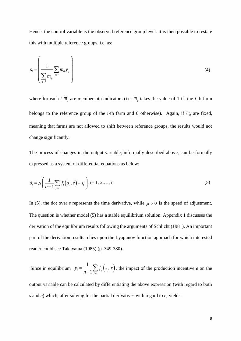
Hence, the control variable is the observed reference group level. It is then possible to restate

this with multiple reference groups, i.e. as:

1i ij j

j iij

j i

s m y

m

(4)

where for each i ijm are membership indicators (i.e. ijm takes the value of 1 if the j-th farm

belongs to the reference group of the i-th farm and 0 otherwise). Again, if ijm are fixed,

meaning that farms are not allowed to shift between reference groups, the results would not

change significantly.

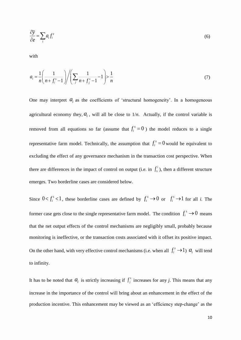
The process of changes in the output variable, informally described above, can be formally

expressed as a system of differential equations as below:

1

,1

i i j i

j i

s f s e sn

, i= 1, 2,…, n (5)

In (5), the dot over s represents the time derivative, while 0 is the speed of adjustment.

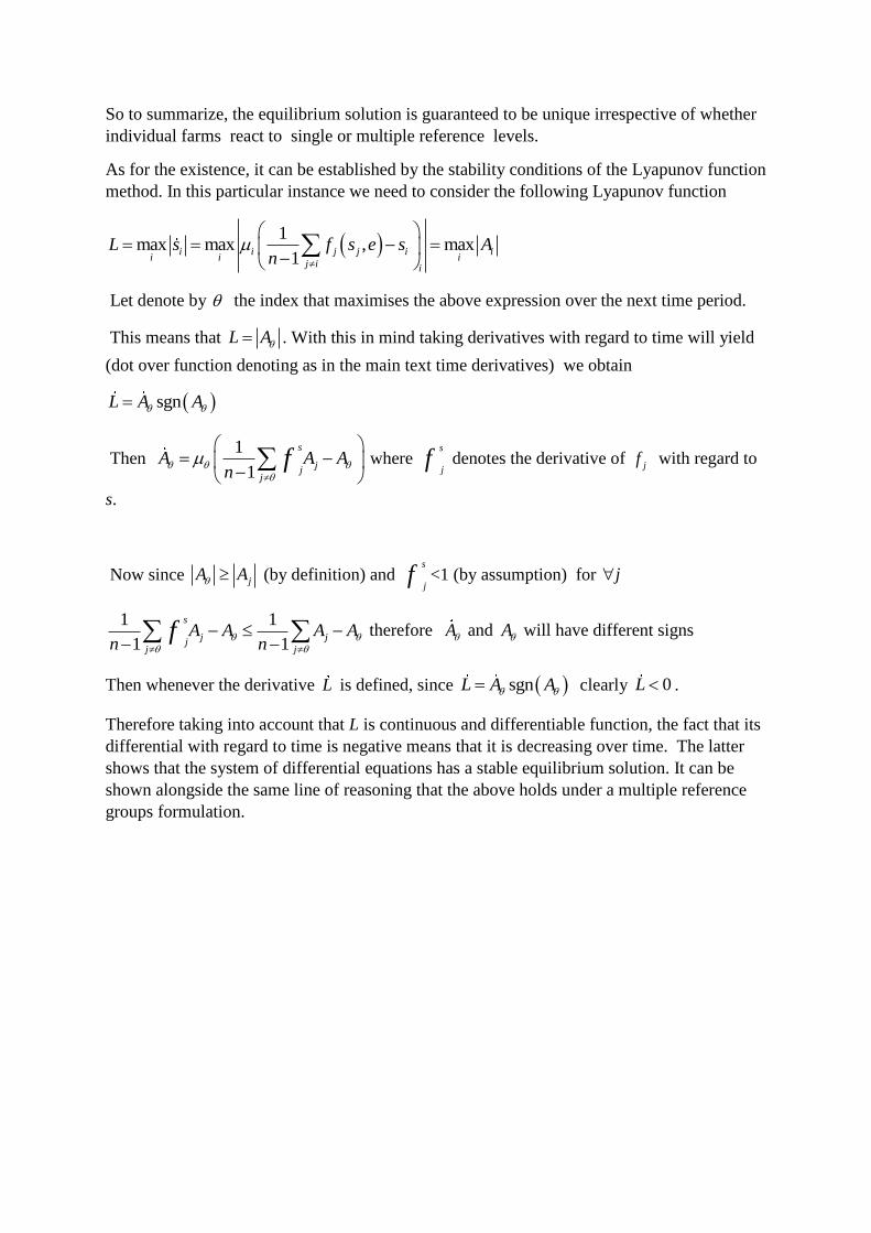
The question is whether model (5) has a stable equilibrium solution. Appendix 1 discusses the

derivation of the equilibrium results following the arguments of Schlicht (1981). An important

part of the derivation results relies upon the Lyapunov function approach for which interested

reader could see Takayama (1985) (p. 349-380).

Since in equilibrium 1

,1

i j j

j i

y f s en

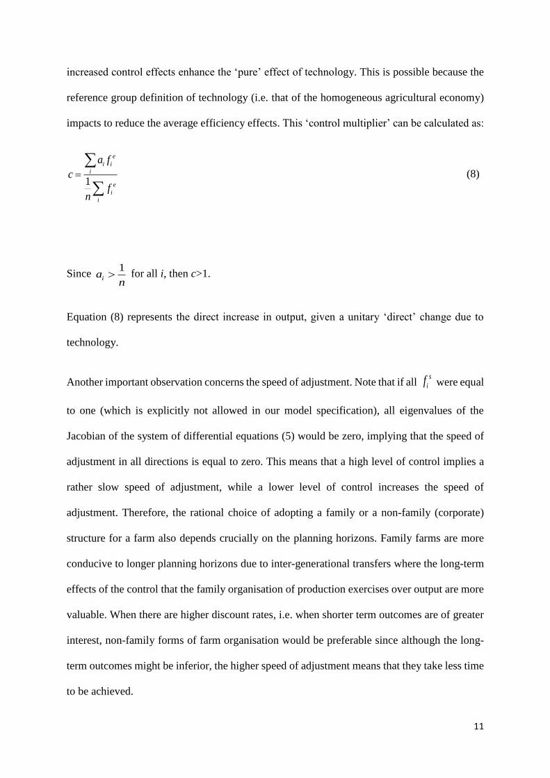
, the impact of the production incentive e on the

output variable can be calculated by differentiating the above expression (with regard to both

s and e) which, after solving for the partial derivatives with regard to e, yields:

10

e

i i

i

ya f

e

(6)

with

1 11 11

1 1i s s

ji j

an f n fn n

(7)

One may interpret ia as the coefficients of ‘structural homogeneity’. In a homogeneous

agricultural economy they, ia , will all be close to 1/n. Actually, if the control variable is

removed from all equations so far (assume that 0s

if ) the model reduces to a single

representative farm model. Technically, the assumption that 0s

if would be equivalent to

excluding the effect of any governance mechanism in the transaction cost perspective. When

there are differences in the impact of control on output (i.e. in i

sf ), then a different structure

emerges. Two borderline cases are considered below.

Since 0 1s

if , these borderline cases are defined by 0s

if or 1s

if for all i. The

former case gets close to the single representative farm model. The condition 0s

if means

that the net output effects of the control mechanisms are negligibly small, probably because

monitoring is ineffective, or the transaction costs associated with it offset its positive impact.

On the other hand, with very effective control mechanisms (i.e. when all 1s

if ) ia will tend

to infinity.

It has to be noted that ia is strictly increasing if s

jf increases for any j. This means that any

increase in the importance of the control will bring about an enhancement in the effect of the

production incentive. This enhancement may be viewed as an ‘efficiency step-change’ as the

11

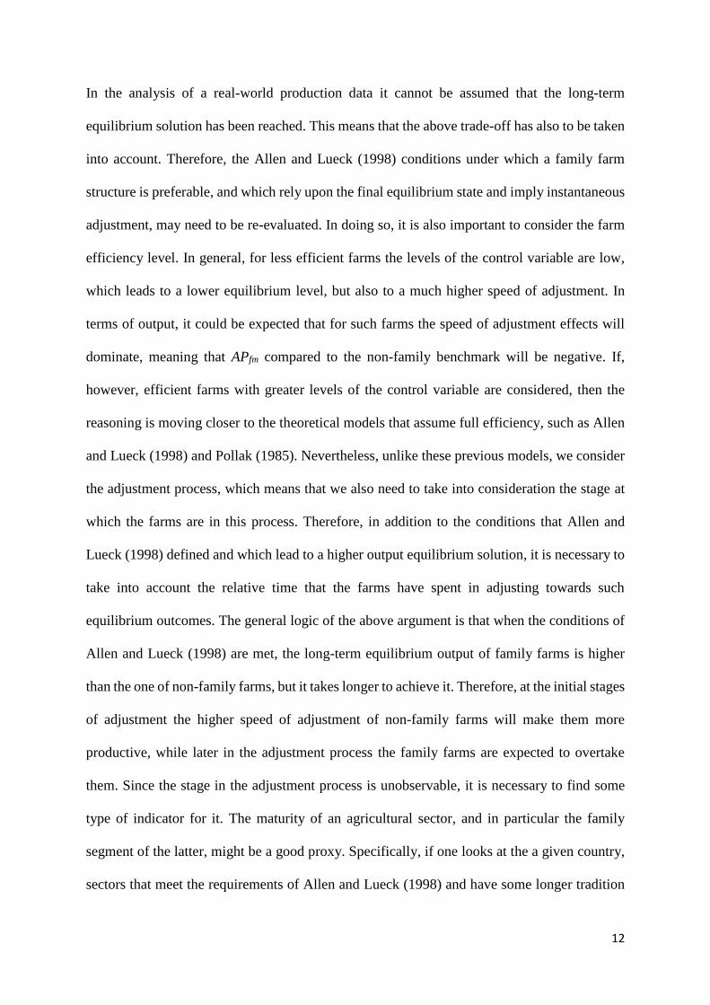
increased control effects enhance the ‘pure’ effect of technology. This is possible because the

reference group definition of technology (i.e. that of the homogeneous agricultural economy)

impacts to reduce the average efficiency effects. This ‘control multiplier’ can be calculated as:

1

e

i i

i

e

i

i

a f

c

fn

(8)

Since 1

ian

for all i, then c>1.

Equation (8) represents the direct increase in output, given a unitary ‘direct’ change due to

technology.

Another important observation concerns the speed of adjustment. Note that if all s

if were equal

to one (which is explicitly not allowed in our model specification), all eigenvalues of the

Jacobian of the system of differential equations (5) would be zero, implying that the speed of

adjustment in all directions is equal to zero. This means that a high level of control implies a

rather slow speed of adjustment, while a lower level of control increases the speed of

adjustment. Therefore, the rational choice of adopting a family or a non-family (corporate)

structure for a farm also depends crucially on the planning horizons. Family farms are more

conducive to longer planning horizons due to inter-generational transfers where the long-term

effects of the control that the family organisation of production exercises over output are more

valuable. When there are higher discount rates, i.e. when shorter term outcomes are of greater

interest, non-family forms of farm organisation would be preferable since although the long-

term outcomes might be inferior, the higher speed of adjustment means that they take less time

to be achieved.

12

In the analysis of a real-world production data it cannot be assumed that the long-term

equilibrium solution has been reached. This means that the above trade-off has also to be taken

into account. Therefore, the Allen and Lueck (1998) conditions under which a family farm

structure is preferable, and which rely upon the final equilibrium state and imply instantaneous

adjustment, may need to be re-evaluated. In doing so, it is also important to consider the farm

efficiency level. In general, for less efficient farms the levels of the control variable are low,

which leads to a lower equilibrium level, but also to a much higher speed of adjustment. In

terms of output, it could be expected that for such farms the speed of adjustment effects will

dominate, meaning that APfm compared to the non-family benchmark will be negative. If,

however, efficient farms with greater levels of the control variable are considered, then the

reasoning is moving closer to the theoretical models that assume full efficiency, such as Allen

and Lueck (1998) and Pollak (1985). Nevertheless, unlike these previous models, we consider

the adjustment process, which means that we also need to take into consideration the stage at

which the farms are in this process. Therefore, in addition to the conditions that Allen and

Lueck (1998) defined and which lead to a higher output equilibrium solution, it is necessary to

take into account the relative time that the farms have spent in adjusting towards such

equilibrium outcomes. The general logic of the above argument is that when the conditions of

Allen and Lueck (1998) are met, the long-term equilibrium output of family farms is higher

than the one of non-family farms, but it takes longer to achieve it. Therefore, at the initial stages

of adjustment the higher speed of adjustment of non-family farms will make them more

productive, while later in the adjustment process the family farms are expected to overtake

them. Since the stage in the adjustment process is unobservable, it is necessary to find some

type of indicator for it. The maturity of an agricultural sector, and in particular the family

segment of the latter, might be a good proxy. Specifically, if one looks at the a given country,

sectors that meet the requirements of Allen and Lueck (1998) and have some longer tradition

13

of specialisation would build competitive advantage which would signify that they are further

on their adjustment path and, therefore, it is expected that family farming at this point of time

would be more productive.

Let us consider, for example, condition 4 of Allen and Lueck (1998) which states that under

higher uncertainty family farming is preferable. Indeed, since the speed of adjustment under

family farming will be lower, it will smoothen the output path reducing variability.

Concurrently, the ‘control multiplier’ will assume higher values leading to higher long-term

equilibrium output. However, in the short term, this resilience to external shocks will reduce

the ability to take advantage of favourable opportunities and when such shock or uncertainty

persist, the short-term disadvantages will dominate, resulting in family farms experiencing

negative APfm in comparison to non-family.

Based on the arguments presented above, on the one hand, there are reasons to hypothesise that

under certain circumstances family farms would be a superior form of organisation and would

hence provide productivity gains over corporate farming. This is the main message based on

the transaction cost approach. In this paper this is termed a motivation hypothesis. Furthermore,

since the study uses the amount of family labour employed as an indicator of how much a farm

is rooted into the family tradition, we explicitly hypothesise that the motivational aspects will

strengthen with a higher level of family orientation, i.e. in this case with a higher use of family

labour. In other words, in its pure form the motivation hypothesis would lead to a positive APfm

and this contribution is expected to increase with the use of family labour.

On the other hand, there could be negative production effects due to the prevalence of social,

as opposed to economic, considerations in family farming that could render corporate farm

organisations superior. The type of effects dominant here is not, however, inconsistent with the

transaction costs approach (see e.g. Pollak, 1985 who notes the possible multi-objective nature

14

of family farms). There are different reasons why such social considerations can lead to

suboptimal output outcomes. For example, non-economic objectives would distract the

management from achieving purely economic outcomes, hence potentially reducing output.

This latter type of effect is termed here as the management capabilities deterioration

hypothesis. The main reason for using such a term is that from a corporate governance

perspective a social type of motivation would result in reduced capability to achieve economic

aims. Similarly to the previous case, it can be further hypothesised that when a farm becomes

more family oriented, the importance of such non-economic aims may increase, resulting in a

larger negative effect on the output.

Both these hypotheses are consistent with the theoretical model presented above. As mentioned

previously, family farming would likely generate a greater level of control consistent with the

motivation hypothesis, but also a lower speed of adjustment toward the steady state, which

leads to a negative impact as hypothesised by the management capabilities deterioration

hypothesis. Which one will dominate will depend on the trade-off between the steady state and

the speed of adjustment. In a dynamic perspective, as adopted in the theoretical model, the

motivation hypothesis associated with the steady state is more likely to hold in more mature

sub-sectors, as a longer established sub-sector can be expected to have undergone most of the

transition towards the steady state. Less mature sub-sectors, however, would likely be further

away from the steady state and hence the speed of adjustment will dominate the determination

of the effects, with the consequence that the lower speed of adjustment of family farms would

lead to a negative APfm consistent with the management capabilities deterioration hypothesis.

These effects are, however, unlikely to be present in such pure forms and the interplay between

the two types of effects will determine whether the relative APfm is positive or negative.

Finally, the relative magnitude of the production effects, irrespective of their pattern, would

depend on the structure of the sector, with a higher degree of structural homogeneity (as

15

expressed by ai in our theoretical model) leading to smaller effects. For example, whenever one

form of farm structure dominates strongly in a country, this would imply a higher level of

homogeneity and therefore smaller APfm would be expected.

Linde (1982) offers an interesting static (steady state equilibrium) result for reference group

models. In the terminology used in the present paper Linde (1982) allows for heterogeneous

response to the production incentive, but does not investigate the existence of equilibrium. As

shown in appendix 1, the dynamics of such a model converges to a unique steady state.

According to Linde (1982), overall optimality is achieved when units with high levels of

production incentive apply high levels of control. This provides an interesting twist to the issue

of family vs non-family farms. Consider this with regard to the issue of technical efficiency.

Since the latter is a product of the production incentive (more efficient farms will have higher

values for the production incentive) and control (in that the higher levels of control lead to

greater efficiency) this result means that these two components are correlated. In simple terms

this means that advantages of the ability to exercise control will most likely manifest

themselves at higher levels of technical efficiency. Therefore, in terms of the assumption that

family farming advantages can result from a higher degree of control, we should expect that

this would be larger at higher levels of technical efficiency.

Furthermore, the advantages of family farming are expected to increase with the additional

level of control that they can achieve. Hereafter, we argue that the level of family involvement

(that we measure by the use of family labour) can proxy such control. This means that we

expect that increased levels of family involvement should increase the advantages of family

farms.

Hence, the implications of the theoretical models are as follows: advantages of family over

corporate farming are likely to be dependent on the distance to steady state (which will be

16

greater and hence such advantages smaller, if there was a recent economic shock), the level of

structural homogeneity (generally unobservable, but can in some case be deduced from

empirical results), the level of technical efficiency and the family involvement. In the empirical

application we explicitly account for the last two and the discussion of the results throws some

light upon the other factors.

III. Definitional issues

‘Family farm’ and ‘family farmer’ may be defined in several ways. Definitions can be based

on absolute amount or the share of family labour used in the total labour input, on ownership

and control (and thus succession between generations), on legal status (sole holders), or on who

bears the business risk (Davidova and Thomson, 2014).

During the debate in relation to the IYFF, FAO proposed that a family farm is an agricultural

holding which is managed and operated by a household and where farm labour is largely

supplied by that household (FAO, 2013). One important point in this definition is the emphasis

on the operational aspect of the farm, i.e. the use of family labour.

Several attempts have been made to define quantitative thresholds of the family labour in order

to delineate the family farm sector. Matthews (2013) suggests that family farmers are those

who are farming with labour input of up to 2 Annual Work Units (AWUs), since this may

represent full-time employment of a farmer with spouse, or with daughter/or son, or with one

hired worker. Hill (1993) defines three groups of farms: first, family farms where the share of

family labour, measured in AWUs, is at least 95 per cent of all full-time labour; second,

intermediate farms with between 50 and 95 per cent of family labour, and third, non-family

farms where the holder and family members contribute less than 50 per cent of the labour.

17

This study departs from the proportional (share) definition in light of the adopted theoretical

framework. As already discussed, what makes a family farm is not the share of family to non-

family labour, but the nature of the governance/monitoring mechanisms that the family

involvement implies. Hence, from a governance perspective, what makes a farm a family farm

is the fact that family labour is actively involved in mitigating monitoring problems and

ensuring effective governance. In this sense, the involvement of family labour is better

measured by its absolute quantity rather than its share.

IV. Empirical methodology

The empirical approach employs a non-parametric quantile regression. The quantile regression

estimates the conditional distribution of the dependent variable with regard to a set of

covariates. Since the conditional quantiles are, in general, different from the unconditional

ones, it is necessary to highlight some points which are important for the interpretation of the

estimates which follow. The particular interpretation depends on the nature of the conditional

relationship that is being estimated. In this study production functions are estimated. In this

regard, upper conditional quantiles refer to farms which are able to extract more output from

their given endowments, i.e. the inputs in the production function, than other comparable farms

and vice versa. Hence, the conditional output distribution inferred from a production function

measures the unobservable farm ability to transform inputs into output, thus it measures

technical efficiency. The upper tail of this conditional distribution denotes more efficient farms

while the lower tail refers to the least efficient ones.

Here the unknown production function is estimated non-parametrically and thus avoids the

necessity to specify any pre-defined functional form for production. The nonparametric

quantile regression applied here can be expressed as:

y f X u (9)

18

st | 0q u X (10)

In contrast to the more widely known linear quantile regression specification (e.g. Koenker,

2005) the effect of the covariates is given by a non-parametrically specified function, which

itself is quantile dependent, and the conditional quantile restriction in (10) is specified with

regard to this non-parametric function (see Li and Racine, 2007). There are two important

consequences from the above. First, the effects of a particular input are given by a functional

relationship, which will assign a set of values for such effects. Second, unless additivity of the

effects of the production function is assumed, something that is clearly undesirable, then the

implied nonadditivity means that any effect will need to be calculated by, and conditioned on,

some kind of averaging over the dataset.

At this stage, in order to facilitate interpretation, it would be useful to contrast the quantile

regression method to that of the more familiar mean regression. In mean regression the

equivalent to (10) is something like

2~ (0, )u N (11)

Which is a combination of 0E u and means that the functional relationship (9) being

estimated applies to the conditional mean and some distributional assumption about the

residuals. This would typically be a Gaussian distribution with a constant variance as in (11)

above, although a variety of alternative distributional assumptions can be used instead. This

has two important implications. First, the same relationship is essentially applicable to all

observations in the sample and the residuals from it represent the conditional distribution y|X.

This conditional distribution has an associated distributional assumption (usually Gaussian, as

above, but alternative assumption could be used instead). In conditional quantile regression,

the conditional quantile restriction in (10) specifies that the functional relationship (in (9))

refers to the respective conditional quantile. In other words we estimate a relationship that only

19

applies at a given point of the conditional quantile distribution. Since we do not assume

anything about the quantile residuals (derived from applying (9)), they do not have the

interpretation of conditional distribution. However the quantile method allows one to estimate

the whole conditional distribution of y given X. This could be done by estimating the quantile

process, which technically means estimating as many quantile regressions as the number of

observations in the sample. If one does this then effectively, a different functional relationship

(9) will be estimated for each observation.

There are various nonparametric extensions of the quantile regression model, using e.g. kernel

approaches (Li et al., 2007), inversion of nonparametrically estimated conditional density (Li

and Racine 2008), local estimation (Yu and Jones, 2008), smoothing splines (Koenker et al.,

1994, Thompson et al., 2010), penalised variograms (Koenker and Mizera, 2003) and

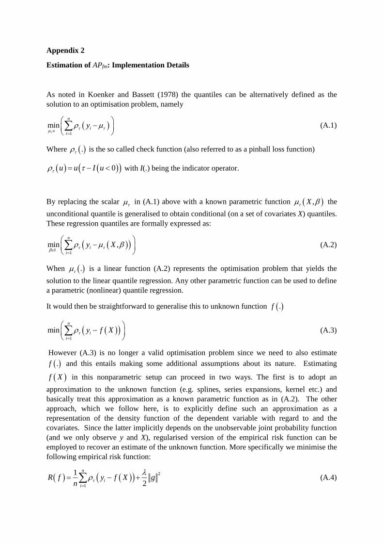
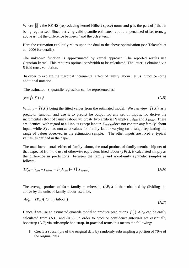
algorithmic approximation (Jiang, 2014).3 This paper adopts the approach of Takeuchi et al.

(2006) who show that the optimisation problem of non-parametric quantile regression, when

specified via regularisation based on reproducing kernel Hilbert spaces norm, bears

resemblance to the approach widely used in the machine learning support vector regression. In

fact, it is a simplified version of the 𝜀-support vector machine regression problem.

Technically, unlike the standard support vector regression, which requires pivoting, the

estimates can be calculated by standard quadratic optimisation methods. This modelling

approach is more amenable to the problem at hand since non-additivity is implicitly accounted

for rather than being represented more explicitly in terms of higher order interaction surfaces

as required in the kernel and spline approaches. This particular alternative has the important

advantage of maintaining a lower computational workload and relative robustness with regard

3 Since imposing additivity on the farm production function is undesirable and unjustified, the extensive

literature on additive semi- and non-parametric quantile regression models is not used in this study.

20

to the estimation of the (conditional) densities.4 Cementing our choice of modelling approach,

this particular choice is that, once the corresponding models are estimated, predicting from

them is much simpler than with most alternative methods.

The paper employs Gaussian kernels to specify the reproducing kernel Hilbert spaces for the

regularisation norm and a 5-fold cross-validation to select the optimal parameters. The latter is

the main source of computational costs. The robustness of the results of this essentially novel

application to an empirical problem is likely to be of particular concern to readers. We,

therefore, felt that a multi-fold cross-validation was necessary in view of the computational

complexity of the estimation problem and, thus, the additional computational costs were

justified on these grounds.

Two separate types of nonparametric quantile regressions were estimated at the 0.9th and the

0.1th quantiles. Since the former refers to farms which are more efficient than 90 per cent of

the comparable farms and the latter refers to farms that are less efficient that 90 per cent of the

other farms, hereinafter the two quantiles are simply referred to as ‘efficient’ and ‘inefficient’

farms. Intentionally, the analysis does not go too deep into the tails of the conditional

distribution to eliminate the potential effect of outliers. As discussed in the theoretical model

we expect that the advantages of family farming will manifest themselves at higher levels of

technical efficiency.

Estimating via nonparametric quantile regression the whole quantile process would provide

estimates for every farm in the sample. While theoretically and conceptually a 90 per cent

technically efficient farm refers to a single farm in the estimation sample (for which the residual

4 Given the computational requirements of the estimations, computational load has been an important

consideration. The only estimation method with lower computational costs we were able to identify was

that of Kriegler and Berk (2010), but it is based on a boosting framework that is relatively less well-

known and the estimation process involves some fine tuning, description of which would distract from

the main focus of the paper.

21

in (10) for =0.9 is zero), the nonparametric quantile regression provides point estimates for

every single farm in the dataset, i.e. the unknown relationship f X is estimated over all

farms. This means that the nonparametrically derived estimates for the relationship in (9) are

derived at all points in the estimation sample. The interpretation of the result form this

functional relationship shows what the output would be for every single farm if it had achieved

that particular level of technical efficiency. In other words, although by fixing the conditional

quantile we estimate a single point of the conditional distribution, the estimation then allows

us to infer the production response of an efficient (or inefficient) farm as the mix of its inputs

changes. Given the estimation this means that ˆy f X gives us estimates of what the output

of any given farm would have been if it had the pre-specified (e.g. 90%) level of technically

efficiency. Alternatively by applying the same to a different dataset or a farms descriptions in

terms of mix of inputs, the same question could be answered.

In a way this is not that different from what efficient frontier models (which technically are

100% quantile models) provide in that they allow one to specify what would be the optimal

(i.e. maximum) output level for each farm. Here in contrast we can specify for any farm how

its output would change with the level of technical efficiency (provided of course we estimate

different quantile regression models for all such efficiency levels of interest).

In this study the interest is not on the overall production response, but on how it changes with

regard to a particular input. If the additive model formulation was adopted, the overall

production response could be split amongst the inputs (since in this case ,

1

k

j j

j

f X f X

for all inputs j=1, 2,…, k). With a non-separable production function the above is no longer

possible and any effects have to be conditioned with regard to a reference sample. In simple

terms, this means that the production response of, for example, an efficient farm for any given

22

mix of inputs could be estimated by a simple prediction from an estimated nonparametric (in

this case 0.9th) quantile regression model. The effect of any particular input can therefore be

obtained by creating an artificial prediction sample in which the values for this particular input

are varied, but all other inputs are fixed at some ‘typical’ values. The resulting partial

correlation effects will provide the ‘typical’ effects of the input of interest. Such a procedure

would result in point estimates for the required effects while confidence intervals can be

constructed by bootstrap (see Kostov et al., 2008).

A standard approach to defining what is ‘typical’ involves simply averaging all the other

variables over the estimation sample and this approach is implemented in this paper5. However,

one has to be careful when averaging variables, particularly in non-separable models, since

averaged combination of variables can still be atypical and a careful consideration should be

given to both the feasibility and meaning of these combinations. In this study the focus is on

the effect of family labour. By standard averaging a synthetic reference farm that has the

average stock of the other inputs is obtained. However, such an input mix might be unusual for

a family farm. Economic efficiency arguments mean that only certain combinations of the other

inputs would be conducive to using family labour. To correct for this, a second alternative

approach is applied to create a reference. This involves averaging of the other inputs only over

the family farms, i.e. the farms with non-zero family labour input. In this way a ‘typical’ family

farm is created. This might be more realistic since it studies the effect of family labour for an

input mix that is feasible for family farms.

5 It has to be noted that production function relationships can be characterised by complex trade-offs

amongst inputs, trade-offs that are likely to be non-linear and conditional on the overall input mix.

Using a linear operator, such as averaging, to construct the reference sample will inevitably simplify

this complexity.

23

In essence the effects we calculate and present hereafter are counterfactual effects. They are

counterfactual in that they are derived from the difference between their output and that which

could be gained from otherwise identical family and non-family farms as appropriate. If such

effects were to be directly estimated form the data the results would have been classified as

quantile ‘treatment effects’ and issues of identification would have arisen. While identification

results for additive treatment effects exist, to the best of our knowledge no such results has

been established for non-separable models. No such problems however exist in the

counterfactual distributions analysis (see Chernozhukov et al., 2013 for additive models) which

distinguishes type 1 counterfactual effects (effects based on changing the conditional

distribution), type 2 (changing the covariate structure) and type 3 effects (which are based on

changing both conditional distribution and covariate structure). The counterfactuals we use

here are type 1 in the above terminology, and by their nature they require us to fix the covariate

structure. The main difference is that dues to the non-separable nature of our model we do not

construct the whole distribution of such effects, but instead focus on two distinct points of the

conditional distribution, namely the ‘efficient’ and ‘inefficient’ farms.

Conditioning on a reference sample allows us to calculate the output response to varying family

labour input. The output difference between the reference sample and its non-family equivalent

(i.e. a farm with the same inputs mix, but no family labour) is calculated. This difference,

positive if the family farm output is larger than non-family, or negative in case the non-family

equivalent has larger production, represents the total product of farm family membership (the

TPfm). This incremental contribution is divided by the quantity of family labour to arrive to an

estimate of the APfm expressed per Annual Work Unit (AWU) of family labour. Throughout the

paper we refer to the latter measure as the Average Product of Farm Family Membership (APfm).

The way the reference (prediction) sample is constructed, allows estimating this APfm for

varying degrees of use of family labour. Details on the derivation of APfm are presented in

24

appendix 2. A bootstrap procedure is implemented to derive confidence intervals for APfm.

Since this is a computationally expensive part we have implemented it as a part of the

estimation process, i.e. have estimated all the bootstrapped models and saved them to use for

prediction purposes in the APfm calculations.

V. Data

The data used in the study has been derived from the EU’s Farm Accountancy Data Network

(FADN), 2008. The FADN samples only holdings above a threshold, defined in terms of their

economic size, so the very small (often semi-subsidence) family farms are excluded. The

analysis focuses on four EU Member States which differ substantially according to their farm

structure – the Czech Republic, Hungary, Romania and Spain. The Czech Republic has a

particularly large corporate farm sector, which does not use family labour while Hungary

presents an interesting mix between corporate and family farms. Romania is the EU Member

State with the largest number of small family farms out of which 93 per cent are semi-

subsistence, thus consuming more than half of their output within the household (Davidova et.

al., 2013). Semi-subsistence farms are not included in FADN but in reality they affect the nature

of the commercial farms which are the FADN field of observation. Finally, Spain’s agriculture

is dominated by family farms.

Altogether, these four countries account for 12,929 observations in the EU FADN dataset, out

of which 11,606 are family farms (89.7 per cent of all observations). There is a clear divide

between the EU New Member States (NMS) and Spain. Although in all four case study

countries family farms are predominant in the total number of farms, their share in total land

cultivated by FADN sample farms and in total labour input in the Czech Republic, Hungary

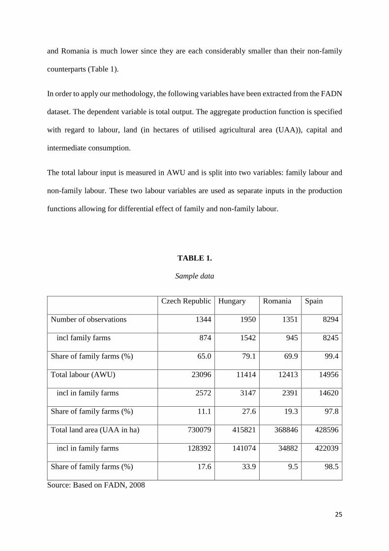
25

and Romania is much lower since they are each considerably smaller than their non-family

counterparts (Table 1).

In order to apply our methodology, the following variables have been extracted from the FADN

dataset. The dependent variable is total output. The aggregate production function is specified

with regard to labour, land (in hectares of utilised agricultural area (UAA)), capital and

intermediate consumption.

The total labour input is measured in AWU and is split into two variables: family labour and

non-family labour. These two labour variables are used as separate inputs in the production

functions allowing for differential effect of family and non-family labour.

TABLE 1.

Sample data

Czech Republic Hungary Romania Spain

Number of observations 1344 1950 1351 8294

incl family farms 874 1542 945 8245

Share of family farms (%) 65.0 79.1 69.9 99.4

Total labour (AWU) 23096 11414 12413 14956

incl in family farms 2572 3147 2391 14620

Share of family farms (%) 11.1 27.6 19.3 97.8

Total land area (UAA in ha) 730079 415821 368846 428596

incl in family farms 128392 141074 34882 422039

Share of family farms (%) 17.6 33.9 9.5 98.5

Source: Based on FADN, 2008

26

Capital is calculated as the difference between total fixed assets, on the one hand, and land,

permanent crops and quotas, on the other. In this way a proxy for a long-term capital is

obtained. The value of the land is excluded from the capital measure in order to avoid double

counting since it is used as a separate input to the production function. FADN bundles together

the value of land with permanent crops and policy quotas, and does not provide information

for the quality of land.

Finally, the total intermediate consumption is extracted as calculated in FADN.

VI. Results

As discussed in the methodology section, in order to present the effect of family labour in a

non-separable production function framework, we need to invoke a ‘reference’ sample

approach where all the other inputs are fixed at some ‘typical’ values. Here we apply two

separate approaches to constructing such a reference sample, which we present separately.

VI.A. Conventional reference sample

In the conventional reference sample, all the other inputs are averaged over the whole data

sample. The estimated APfm in the Czech Republic, Hungary, Romania and Spain are presented

in Figure 1. Since very small values of family labour could signify occasional ad hoc use and

may result in high variability of the estimated effects, only values of family labour of at least

0.5 AWU are used.

27

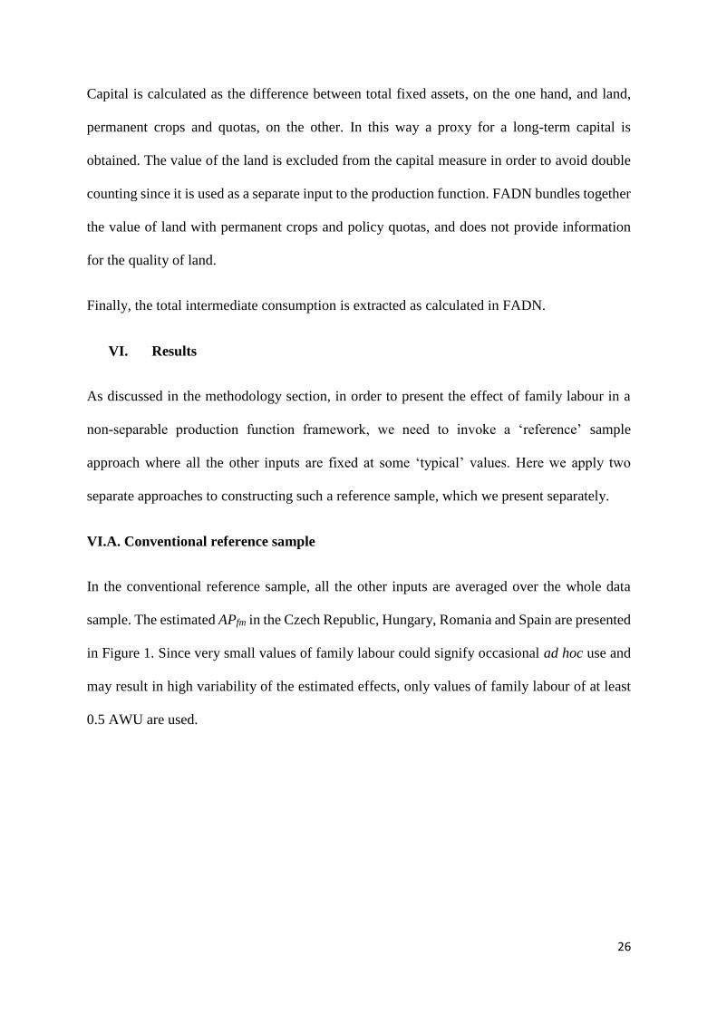
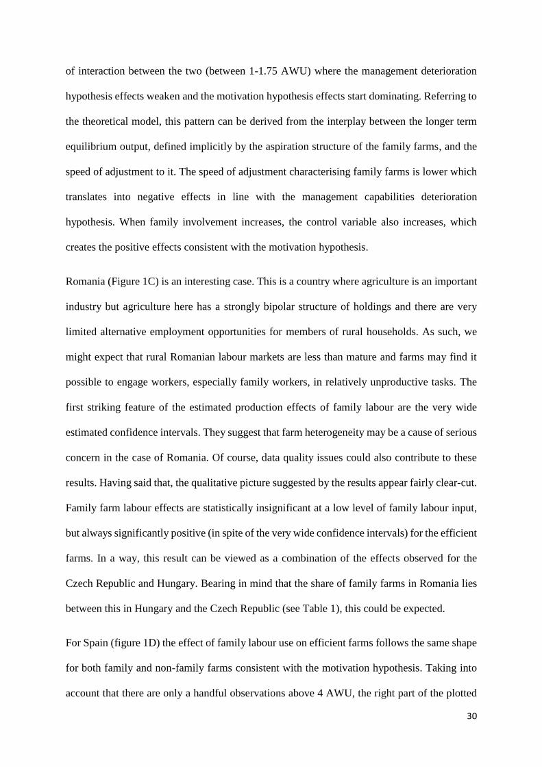
Figure 1. Estimated effects of family labour

The values of family labour in the synthetic reference sample, used for calculating the effects

of interest, are a regular grid over the range of observed values in the data. However, these

values are not uniformly distributed across the estimation sample. When the estimation sample

only contains a few observations within a specific range, the estimated effects pertaining to this

particular range should be treated with caution since they lack sufficient data support. For these

reasons, the estimated effect is presented in rug plots, where rugs (vertical lines) are added to

the horizontal axis to denote the empirical support for the corresponding estimates. The rugs

are derived from the data used to estimate the effects, i.e. the rugs denote the corresponding

observations in the estimation sample. In this case they are plotted at the values for the

horizontal axis, i.e. family labour. In this way, it is straightforward to visualise where there is

relative scarcity of data. For example, in all graphs in Figure 1, there are limited number of

observations above 3AWU of family labour.

28

There is however, a difference from what our figures show and the standard practice.

Conventionally both the estimated effects and the rugs are derived from the same data (i.e. the

estimation sample). Here the effects are calculated from a bootstrapped set of non-parametric

quantile regression models, used to predict from the reference sample, while the rugs belong

to the estimation dataset, i.e. they are based on essentially different (respectively prediction

and estimation) datasets. Since the prediction phase uses estimated effects (which themselves

are derived from the estimation dataset) the rug plots are essentially a visualisation device to

ascertain the empirical support for these estimated effects and therefore could be interpreted

accordingly.

In the nutshell, the APfm is neither always statistically significant nor positive. The effect

depends to a great extent on the level of farm efficiency. The differences in the effects on

efficient and inefficient farms are quite large in most instances. Since, as it was argued

previously, the level of efficiency can also be viewed as a measure of the managerial

capabilities, these differences support the expectations that such management capabilities are

crucial in determining the production effect of family labour. The results for inefficient farms

confirm the predictions of the theoretical model and show a negative relative APfm.

Two distinct shapes are observed for the efficient farms. The first one is a positive effect

decreasing with the increase of family labour used and reaching a saturation level, as in the

case of the Czech Republic and Romania. Such an effect is consistent with the motivation effect

hypothesis. However, engaging family members in farming, beyond some threshold, may mean

engaging lower skilled persons for non-economic reasons and this may offset or degrade the

positive governance effects. It has been reported that often family farms retain surplus labour,

whilst non-family farms are more flexible in their employment of unskilled workers.

29

The second observed shape for efficient farms basically replicates the response shape observed

in inefficient farms (see Hungary and Spain). This shape might best be described as a

‘dampened’ motivation hypothesis. A positive effect for the family labour emerges, but this

effect flattens after a certain threshold of family labour input at about 2.8 and 3.6 AWU

respectively. The flattening of the effect may also be simply due to the nature of the data. Since

family labour is subject to constraints in availability in absolute number terms, very large

values may infrequent and, in cases, associated with data quality issues.

On the background of these general results, some country differences provide interesting

insights.

In the Czech Republic, where most of the output is produced by corporate farms and only 11

per cent of the labour input can be accounted for by family farms (Table 1), the effect of family

labour is positive, but relatively small for the efficient farms, while it is very large and negative

for the inefficient farms. In the latter case, even when the use of family labour is increased, its

effect still remains negative (Figure 1A). The small positive effect for efficient farms appears

to be quite stable. This is consistent with the structural homogeneity argument, presented in the

theoretical model, since the Czech Republic agriculture is dominated by corporate farms.

For Hungary (Figure 1B) the effect of family labour for inefficient farms is significantly

negative. The effect for efficient farms exhibits a downward slope at a low use of family labour,

which reduces the positive effect making it insignificant, but at a threshold of around 1AWU

the slope reverses and the effect become significantly positive at approximately 1.75 AWU.

After 2.6 AWU the effect flattens. This type of effect is likely produced by a combination of

management capabilities deterioration hypothesis at lower levels of family labour use where

the APfm is negative and downward sloping, and the motivation hypothesis at higher levels

where this contribution is positive and generally increasing. There is also an intermediate range

30

of interaction between the two (between 1-1.75 AWU) where the management deterioration

hypothesis effects weaken and the motivation hypothesis effects start dominating. Referring to

the theoretical model, this pattern can be derived from the interplay between the longer term

equilibrium output, defined implicitly by the aspiration structure of the family farms, and the

speed of adjustment to it. The speed of adjustment characterising family farms is lower which

translates into negative effects in line with the management capabilities deterioration

hypothesis. When family involvement increases, the control variable also increases, which

creates the positive effects consistent with the motivation hypothesis.

Romania (Figure 1C) is an interesting case. This is a country where agriculture is an important

industry but agriculture here has a strongly bipolar structure of holdings and there are very

limited alternative employment opportunities for members of rural households. As such, we

might expect that rural Romanian labour markets are less than mature and farms may find it

possible to engage workers, especially family workers, in relatively unproductive tasks. The

first striking feature of the estimated production effects of family labour are the very wide

estimated confidence intervals. They suggest that farm heterogeneity may be a cause of serious

concern in the case of Romania. Of course, data quality issues could also contribute to these

results. Having said that, the qualitative picture suggested by the results appear fairly clear-cut.

Family farm labour effects are statistically insignificant at a low level of family labour input,

but always significantly positive (in spite of the very wide confidence intervals) for the efficient

farms. In a way, this result can be viewed as a combination of the effects observed for the

Czech Republic and Hungary. Bearing in mind that the share of family farms in Romania lies

between this in Hungary and the Czech Republic (see Table 1), this could be expected.

For Spain (figure 1D) the effect of family labour use on efficient farms follows the same shape

for both family and non-family farms consistent with the motivation hypothesis. Taking into

account that there are only a handful observations above 4 AWU, the right part of the plotted

31

effects (where they flatten out and decrease) for the efficient farms, can be ignored. For

efficient farms, the effect becomes positive when family labour use exceeds 2.25AWU and

peaks at around 3AWU. This threshold level is higher than in the case of Hungary, where a

similar type of effect was observed. The effect is entirely negative for inefficient farms.

VI.B. Family farms reference sample

As it was already discussed, the above effects are calculated by a reference approach in which

the other inputs are averaged across the whole sample. The second alternative approach is to

average inputs only over the family farms. The family labour effects, estimated using this

alternative ‘family farms only’ approach, are presented in Figure 2.

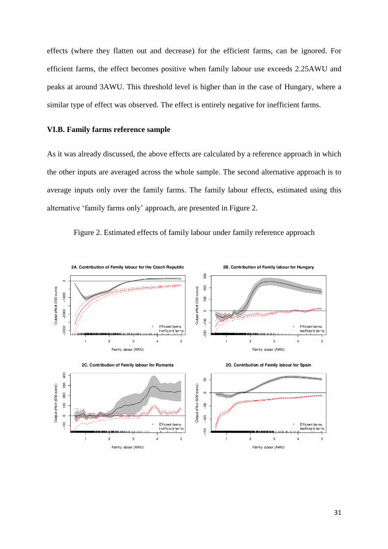
Figure 2. Estimated effects of family labour under family reference approach

32

In the case of the Czech Republic (Figure 2A) the effects for inefficient farms are by and large

unchanged, however, the corresponding effects for the efficient farms look very different.

Family labour no longer appears as an attractive proposition even for the most efficient farms.

The threshold at which the effect for the efficient farms becomes positive is quite high

(approximately 3.5AWU) and although it is statistically significant, it is negligibly small. In an

agriculture dominated by large corporate farms it is more difficult to discover positive effects

for family farm labour and such effects only manifest themselves when the characteristics of

these family farms approach those of the corporate farms, i.e. when they are large.

For Hungary efficient farms exhibit a negative effect, which however is only marginally

significant, up to a threshold of approximately 1.25 AWU when it becomes insignificant. The

second threshold is around 1.75AWU when this effect not only becomes significant and

positive, but increases considerably (Figure 2B). The largest production effect is observed at

approximately 2.5 AWU of family labour input. This suggests that any positive effects of

family labour are only manifested once almost two family members are fully employed on the

farm. The dramatic increase in the effect around 2 AWU indicates that farms which are

essentially family businesses are much more likely to be able to make efficient use of their

family labour input. Beyond the peak in the family labour effect it starts decreasing and this

decrease becomes significant beyond 3 AWU, consistent with the management capabilities

deterioration hypothesis. However, since there are only a handful of observations within the

range of above 3 AWU, which might be due to an outlier effect or a measurement error, the

effects beyond 3 AWU should, therefore, be treated with caution. Furthermore, such a large

use of family labour has a very limited practical applicability since few families have such

labour endowments. The effect of family labour for inefficient farms is negative as suggested

by the theoretical model. It only becomes statistically significant at around 3 AWU, but there

are only a few data observations to support that range. Interestingly, the effects for efficient

33

and inefficient farms are not distinguishable in terms of statistical significance within the range

of up to 1.25 AWU. After this threshold, the effect for efficient farms not only becomes

insignificant but experiences an upward shift.

The estimated effects for Romania (Figure 2C) change considerably in comparison to the

reference approach in which the other inputs have been averaged across the whole sample.

Both inefficient and efficient farms follow a similar upward slope pattern. The effects appear

almost undistinguishable between the two levels of efficiency at a lower use of family labour

(up to 1.5 AWU) and do not differ substantially up to 2AWU. Furthermore, both these effects

are insignificant. In comparison to the previous case when conditioning on the overall sample,

conditioning only on family farms reduces considerably the confidence intervals. The

remarkable coincidence of the estimated effects for differing levels of technical efficiency at a

lower use of family labour may suggest that Romanian farms using low levels of family labour

are predominantly inefficient. Efficient farms manage to achieve a positive effect at relatively

high levels of family labour input. Although this needs to be interpreted with caution, there

appears to be some empirical support in the observations which indicate a high family labour

use. The results for Romania seem somewhat similar to those for Hungary, although there

appears to be a more gradual transition as farms become more family involved. Yet the

statistical insignificance of the APfm, except of the cases of a really heavy family involvement,

is a result unique to Romania. It is possible that in addition to data issues and /or unobserved

heterogeneity of farm structures, a characteristic difference from the other case study countries

is the dualistic structure of Romanian agriculture with small number of large farms and large

number of small semi-subsistence farms. Although the latter are outside the scope of FADN,

the important difference in Romania might be between the semi-subsistence and the

commercial sector leading, to a relative homogeneity of the latter and disguising the differences

between family and corporate farms within the commercial agriculture.

34

For Spain (see figure 2D) the family farm only alternative does not affect the results and they

are virtually indistinguishable from those presented in Figure 1D. Therefore, the estimated

effects of family labour do not depend on the type of conditioning used in constructing the

reference sample. This is to be expected since most of the Spanish farms are family farms, so

reconditioning changes little with regard to the reference sample.

VII. Conclusions and policy implications

It is often claimed that family farming is a ‘superior’ form of organisation of agricultural

production compared to the non-family ‘corporate’ farming. The theoretical arguments related

to the superiority of family farming are centred around family labour which could be more

productive and requiring of lower monitoring costs as it is more motivated in its role as a

residual claimant on farm profits (Allen and Lueck, 1998; Pollak 1985). However, using a

dynamic model, two distinct hypotheses about the nature of such effects are identified in this

study; the motivation hypothesis, which is aligned with the transaction costs perspective, and

the management capabilities deterioration hypothesis.

The empirical results reproduced here reveal a pattern that is consistent with the interplay of

these two hypotheses. While the overall pattern is of an increasing average product of farm

family labour use for efficient farms, two specific thresholds indicate the existence and

importance of the management capabilities deterioration effect. The first is that for low values

of family labour use where the aggregate effects are negative, denoting that the negative,

management capabilities deterioration effect, is of greater magnitude than the positive

motivation effect, since the benefits of better governance are low at a low level of family labour

input. The other indicates a flattening of the response in average product of farm family labour

use at a relatively high threshold, which could be explained by an offset of the positive effect

by engagement of more family labour for social and non-economic purposes. Overall, the shape

35

of the estimated average product of farm family membership, which becomes positive over

some range of family labour input for efficient farms, appears to support the motivation

hypothesis. However, the magnitude of these effects is decreasing with the increase in the

relative homogeneity of farm structures, exemplified by e.g. the results for the Czech Republic.

Furthermore the width of the estimated confidence intervals varies considerably with Spain

and the Czech Republic producing narrow confidence intervals and Romania yielding very

wide confidence intervals. It is possible that some of the above could be due to the quality of

the data, but the inherent heterogeneity of the farm structures in Romania may contribute

significantly to such an effect.

Reconditioning the reference approach in which the non-labour inputs are averaged across the

overall estimation sample to the alternative of averaging the non-labour inputs only over the

family farms alters dramatically the results for the EU NMS but appears to leave the results for

Spain unchanged.

The estimation results indicate that the average product of farm family membership on

inefficient farms is either negative or statistically insignificant. Therefore, the family form of

farm organisation appears unable to overcome the disadvantages of technical inefficiency.

Increasing family labour input appears to further decrease the productivity of inefficient farms,

or in the best case, to keep it at the same low level. Maintaining inefficient family farms in

business through the EU CAP support, in particular Pillar 1, can hardly have economic

justification in light of these results. This support helps to bolster farms that fulfil mainly social

functions, such as the preservation of family values, act as a buffer to rural unemployment in

poorer rural regions and slow down rural-urban migration. CAP Pillar 2 rural development

measures in contrast may be more usefully targeted to support family farming. Potentially

useful interventions from Pillar 2 could include the facilitation of inter-generational transfers,

the promotion of structural change through retirement schemes, improving farm efficiency and

36

competitiveness via investments in farm modernisation, and improving the environmental

performance of family farms (Hennessey, 2014). Support to producer groups may also offset

the negligible market power of individual family farmers and facilitate their integration into

the modern food chain may also be of value although this goes beyond the scope of the work

reported here. All these measures could potentially boost the efficiency of family farms and

help to increase the average product of farm family members and to promote a more

sustainable, less policy dependent, future for the family farm as an entity capable of producing

both economic and social benefits.

Or results suggest that a claim that family farms are superior to other forms of organisation in

agriculture can only be made under certain caveats and then only for farms which are relatively

more technically efficient. To use the claim as a simple generalisation, as it so often is, is likely

flawed in most cases.

References:

Allen, D and Lueck, D. (1998) ‘The nature of the farm’, Journal of Law and Economics,

41(2):343-386.

Chernozhukov, V., I Fernández-Val and B. Melly (2013) ‘Inference on Counterfactual

Distributions’, Econometrica, 81 (6), 2205-2268.

Davidova, S., Bailey, A., Dwyer, J., Erjavec, E., Gorton, M. and Thomson, K. (2013) Semi-

subsistence farming – Value and directions of development, study prepared for the European

Parliament Committee on Agriculture and Rural Development. Available at:

http://www.europarl.europa.eu/committees/en/AGRI/studiesdownload.html?languageDocum

ent=EN&file=93390

37

Davidova, S. and Thomson, K. (2014) Family Farming in Europe: Challenges and

Prospects, in-depth analysis for European Parliament Committee on Agriculture and Rural

Development, Brussels. Available at

http://www.europarl.europa.eu/RegData/etudes/note/join/2014/529047/IPOL-

AGRI_NT(2014)529047_EN.pdf

FAO (2013) 2014 IYFF FAO Concept Note (Modified May 9, 2013).

http://www.fao.org/fileadmin/templates/nr/sustainability_pathways/docs/2014_IYFF_FAO_C

oncept_Note.pdf

Hennessy, T. (2014) CAP 2014-2020 Tools to Enhance Family Farming: Opportunities and

Limits, in-depth analysis for European Parliament Committee on Agriculture and Rural

Development, Brussels. Available at

http://www.europarl.europa.eu/RegData/etudes/note/join/2014/529051/IPOL-

AGRI_NT(2014)529051_EN.pdf.

Hill, B. (1993) ‘The ‘myth’ of the family farm: defining the family farm and assessing its

importance in the European community’, Journal of Rural Studies, 9(4), 359-370.

Jiang, Y. (2014) ‘Nonparametric quantile regression models via majorization-minimization

algorithm’, Statistics and Its Interface, 7, 235–240.

Koenker, R. and Bassett, G. (1978) Regression Quantiles, Econometrica, 46, 33-50.

Koenker, R. and I. Mizera, (2003) ‘Penalized Triograms: Total variation regularization for

bivariate smoothing’, Journal of the Royal Statistical Society (B), 66,145-163.

Koenker, R., Ng, P. and Portnoy, S. (1994). ‘Quantile smoothing splines’, Biometrika, 81, 673–

680.

38

Kostov, P. M. Patton and S. McErlean (2008) ‘Non-parametric analysis of the influence of

buyers’ characteristics and personal relationships on agricultural land prices’, Agribusiness,

24(2), 161-176.

Kriegler, B. and R. Berk (2010) ‘Estimating the homeless population in Los Angeles: An

application of cost-sensitive stochastic gradient boosting’, Annals of Applied Statistics, 4(3),

1234-1255

Li Q, Racine J (2008) ‘Nonparametric estimation of conditional CDF and quantile functions

with mixed categorical and continuous data’, Journal of Business and Economic Statistics,

26(4), 423–434.

Li, Y., Liu, Y., and Zhu, J. (2007). ‘Quantile regression in reproducing Kernel Hilbert Spaces’,

Journal of the American Statistical Association, 102, 477, 255-268.

Li Q. and J. Racine (2007). Nonparametric Econometrics. Theory and Practice. Princeton:

Princeton University Press.

Linde R. (1982) ‘Reference group behaviour and economic incentives: An extension of

Schlicht’s Approach’, Journal of Institutional and Theoretical Economics, 138(4), 728-732.

Matthews, A. (2013). Family farming and the role of policy in the EU, capreform.eu blogsite.

Available at: http://capreform.eu/family-farming-and-the-role-of-policy-in-the-eu

Pollak, R. (1985) ‘A transaction cost approach to families and households, J. Econ. Lit, 23,

581-608.

Schlicht, E. (1981). ‘Reference group behaviour and economic incentives: A further remark’.

Journal of Institutional and Theoretical Economics 137: 733-736.

39

Takayama A. (1985) Mathematical Economics, 2nd Edition. Cambridge, Cambridge University

Press.

Takeuchi, I., Q. V. Le, T. D. Sears and A. J. Smola (2006) ‘Nonparametric quantile estimation’,

Journal of Machine Learning Research, 7, 1231-1264.

Thompson, P., Yu. Cai, R. Moyeed, D. Reeve, J. Stander, (2010) ‘Bayesian nonparametric

quantile regression using splines’, Computational Statistics & Data Analysis, 54(4), 1138-

1150.

Yu, K. and Jones, M. C. (1998). ‘Local linear quantile regression’, Journal of the American

Statistical Association, 93, 228-237.

Appendix 1

The system of differential equations needs to be investigated for an equilibrium solution

1

, , 1,2,..,1

i i j j i

j i

s f s e s i nn

(5)

There are two different steps in this: existence and uniqueness. The uniqueness depends on

considerations of convexity (see Schlicht, 1981) and is established by the fact that the

Jacobian of the system of differential equations above has a dominant diagonal (i.e. is a

diagonally dominant matrix).

In the case with multiple reference groups

1

,i ij j j

j iij

j i

s m f s em

(4)

the corresponding systems of differential equations., i.e.

1

, , 1,2,..,i i ij j j i

j iij

j i

s m f s e s i nm

(5.1)

First let us consider (5). The Jacobian of this system of differential equation has diagonal

elements of i while the off-diagonal elements are of the form

1

1

s

i jfn

for j i .

The sum of the off-diagonal elements for the ith row is then is

1

1

s

i j

j i

fn

Then since 1s

jf (see the assumptions) it follows that

1

1

s

i j i

j i

fn

and since i i this proves the dominant diagonal.

For (5.1) the sum of the off-diagonal elements on row i is

ij

j isi iij j ij i i i

j i j iij ij ij

j i j i j i

m

m f mm m m

Therefore we have a dominant diagonal.

So to summarize, the equilibrium solution is guaranteed to be unique irrespective of whether

individual farms react to single or multiple reference levels.

As for the existence, it can be established by the stability conditions of the Lyapunov function

method. In this particular instance we need to consider the following Lyapunov function

1

max max , max1

i i j j i ii i i

j i i

L s f s e s An

Let denote by the index that maximises the above expression over the next time period.

This means that L A . With this in mind taking derivatives with regard to time will yield

(dot over function denoting as in the main text time derivatives) we obtain

sgnL A A

Then 1

1

s

jj

j

A A An

f

where

s

jf denotes the derivative of

jf with regard to

s.

Now since jA A (by definition) and s

jf <1 (by assumption) for j

1 1

1 1

s

j jj

j j

A A A An n

f

therefore A and A will have different signs

Then whenever the derivative L is defined, since sgnL A A clearly 0L .

Therefore taking into account that L is continuous and differentiable function, the fact that its

differential with regard to time is negative means that it is decreasing over time. The latter

shows that the system of differential equations has a stable equilibrium solution. It can be

shown alongside the same line of reasoning that the above holds under a multiple reference

groups formulation.

Appendix 2

Estimation of APfm: Implementation Details

As noted in Koenker and Bassett (1978) the quantiles can be alternatively defined as the

solution to an optimisation problem, namely

1

minn

i

i

y

(A.1)

Where . is the so called check function (also referred to as a pinball loss function)

0u u I u with I(.) being the indicator operator.

By replacing the scalar in (A.1) above with a known parametric function ,X the

unconditional quantile is generalised to obtain conditional (on a set of covariates X) quantiles.

These regression quantiles are formally expressed as:

1

min ,n

i

i

y X

(A.2)

When . is a linear function (A.2) represents the optimisation problem that yields the

solution to the linear quantile regression. Any other parametric function can be used to define

a parametric (nonlinear) quantile regression.

It would then be straightforward to generalise this to unknown function .f

1

minn

i

i

y f X

(A.3)

However (A.3) is no longer a valid optimisation problem since we need to also estimate

.f and this entails making some additional assumptions about its nature. Estimating

f X in this nonparametric setup can proceed in two ways. The first is to adopt an

approximation to the unknown function (e.g. splines, series expansions, kernel etc.) and

basically treat this approximation as a known parametric function as in (A.2). The other

approach, which we follow here, is to explicitly define such an approximation as a

representation of the density function of the dependent variable with regard to and the

covariates. Since the latter implicitly depends on the unobservable joint probability function

(and we only observe y and X), regularised version of the empirical risk function can be

employed to recover an estimate of the unknown function. More specifically we minimise the

following empirical risk function:

2

1

1

2

n

i

i

R f y f X gn

(A.4)

Where . is the RKHS (reproducing kernel Hilbert space) norm and g is the part of f that is

being regularised. Since deriving valid quantile estimates require unpenalised offset term, g

above is just the difference between f and the offset term.

Here the estimation explicitly relies upon the dual to the above optimisation (see Takeuchi et

al., 2006 for details).

The unknown function is approximated by kernel approach. The reported results use

Gaussian kernel. This requires optimal bandwidth to be calculated. The latter is obtained via

5-fold cross validation.

In order to explain the marginal incremental effect of family labour, let us introduce some

additional notation.

The estimated quantile regression can be represented as:

ˆy f X (A.5)

With ˆy f X being the fitted values from the estimated model. We can view f X as a

predictor function and use it to predict he output for any set of inputs. To derive the

incremental effect of family labour we create two artificial ‘samples’, Xfam and Xnonfam. These

are identical with regard to all inputs except labour. Xnonfam does not contain any family labour

input, while Xfam has non-zero values for family labour varying on a range replicating the

range of values observed in the estimation sample. The other inputs are fixed at typical

values, as defined in the paper.

The total incremental effect of family labour, the total product of family membership net of

that expected from the use of otherwise equivalent hired labour (TPfm), is calculated simply as

the difference in predictions between the family and non-family synthetic samples as

follows:

ˆ ˆˆ ˆfm fam nonfam fam nonfamTP y y f X f X (A.6)

The average product of farm family membership (APfm) is then obtained by dividing the

above by the units of family labour used, i.e.

fm fmAP TP family labour (A.7)

Hence if we use an estimated quantile model to produce predictions .f APfm can be easily

calculated from (A.6) and (A.7). In order to produce confidence intervals we essentially

bootstrap (A.7) via subsample bootstrap. In practical terms this means the following:

1. Create a subsample of the original data by randomly subsampling a portion of 70% of

the original data.

2. Estimate the corresponding quantile (0.1 and 0.9) regression model for each of the

subsamples

3. Calculate the APfm for each subsample, by using the predicted values corresponding

quantile model and the two reference samples.

4. Use the (empirical) sampling distribution of the APfm to calculate confidence intervals.

In practical terms steps 1 and 2 and independent of the creation of family and non-family

reference samples needed for step 3. Since this is a computationally expensive part we have

implemented it as a part of the estimation process, i.e. have estimated all the bootstrapped

models and saved them to use for prediction purposes in the APfm calculations