ARTICLE doi:10.1038/nature14469 Resonant interactions and chaotic rotation of Pluto’s small moons M. R. Showalter 1 & D. P. Hamilton 2 Four small moons—Styx, Nix, Kerberos and Hydra—follow near-circular, near-equatorial orbits around the central ‘binary planet’ comprising Pluto and its large moon, Charon. New observational details of the system have emerged following the discoveries of Kerberos and Styx. Here we report that Styx, Nix and Hydra are tied together by a three-body resonance, which is reminiscent of the Laplace resonance linking Jupiter’s moons Io, Europa and Ganymede. Perturbations by the other bodies, however, inject chaos into this otherwise stable configuration. Nix and Hydra have bright surfaces similar to that of Charon. Kerberos may be much darker, raising questions about how a heterogeneous satellite system might have formed. Nix and Hydra rotate chaotically, driven by the large torques of the Pluto–Charon binary. Pluto’s moon Kerberos (previously designated S/2011 (134340)1 or, colloquially, P4) was discovered in 2011 1 using images from the Hubble Space Telescope (HST). It orbits between the paths of Nix and Hydra, which were discovered in 2005 and confirmed in 2006 2 . Follow-up observations in 2012 led to the discovery of the still smaller moon Styx (S/2012 (134340)1 or P5) 3 . The complete data set includes numerous additional detections of both objects from 2010–2012 4–6 , plus a few detections from 2005 (H. A. Weaver, personal commun- ication, 2011) and from 2006 7 ; see Supplementary Table 1. Figure 1 shows samples of the available images. Motivated by these discoveries, we investigate the dynamics and physical properties of Pluto’s four small outer moons. Orbits Pluto and Charon comprise a ‘binary planet’—two bodies, similar in size, orbiting their common barycentre. Their mutual motion creates a time-variable and distinctly asymmetric gravity field. This induces wobbles in the orbits of the outer moons and also drives much slower apsidal precession and nodal regression 8 . In our analysis, we ignore the short-term wobbles and derive time-averaged orbital elements. This is equivalent to replacing the gravity field by that of two con- centric rings containing the masses of Pluto or Charon, each with a radius equal to that body’s distance from the barycentre. We have modelled the orbits using six Keplerian orbital elements (semimajor axis a, eccentricity e, inclination i, mean longitude at epoch l 0 , longitude of pericentre $ 0 , and ascending node V 0 ) plus three associated frequencies (mean motion n, nodal precession rate _ $, and apsidal regression rate _ V). We work in the inertial Pluto–Charon (P–C) coordinate frame, with Pluto and Charon in the x–y plane and the z axis parallel to the system’s angular momentum pole (right ascension 8 h 52 min 5.5 s, declination 26.218u) 6 . We have solved for these elements and frequencies under a variety of assumptions about how they are coupled (Extended Data Table 1). Table 1 lists the most robustly determined elements, in which we enforce a relation- ship that ensures _ $ <{ _ V; this allows us to fit eight elements rather than nine. We prefer this solution because root-mean-square (RMS) residuals are nearly the same as for the solution where _ $ and _ V are allowed to vary independently. Additional possible couplings, invol- ving a and n as well, markedly increase the residuals for Styx and Nix; this suggests that non-axisymmetric gravitational effects, which are not modelled by our concentric ring approximation, can be import- ant. The statistically significant (P-value = 1%) ,100-km residuals of Nix and Hydra (Table 1) match the predicted scale of the un-modelled wobbles 8 , and so are to be expected. Table 1 shows that e and i are distinctly non-zero; this was not apparent in prior work, which employed a different coordinate frame 5 or was based on 200-year averages 6 . Our results describe each moon’s motion during 2005–2012 more accurately. Variations in n, e and i are detectable during 2010–2012 (Extended Data Fig. 1), illustrating the mutual perturbations among the moons that have been used to con- strain their masses 6 . Search for resonances Pluto’s five moons show a tantalizing orbital configuration: the ratios of their orbital periods are close to 1:3:4:5:6 1,3,5,9 . This configuration is reminiscent of the Laplace resonance at Jupiter, where the moons Io, Europa, and Ganymede have periods in the ratio 1:2:4. Table 1 shows the orbital periods P of the moons relative to that of Charon, con- firming the near-integer ratios. However, with measured values for _ $ and _ V in addition to n, it becomes possible to search for more complicated types of resonances. A general resonance involves an angle W~ P j p j l j zq j $ j zr j V j and its time derivative _ W~ P j p j n j zq j _ $ j zr j _ V j . Here, (p j , q j r j ) are integer coefficients and each subscript j is C, S, N, K or H to identify the associated moon. A resonance is recognized by coefficients that sum to zero and produce a very small value of _ W; in addition, the resonant argument W usually librates around either 0u or 180u. Using the orbital elements and their uncertainties tabulated in Table 1, we have performed an exhaustive search for strong reso- nances in the Pluto system. One dominant three-body resonance was identified: W 5 3l S 2 5l N 1 2l H < 180u. This defines a ratio of synodic periods: 3S NH 5 2S SN , where the subscripts identify the pair of moons. We find that _ W520.007 6 0.001u per day and that W decreases from 191u to 184u during 2010–2012; this is all consistent with a small libration about 180u. Note that this expression is very similar to that for Jupiter’s Laplace resonance, 1 SETI Institute, 189 Bernardo Avenue, Mountain View, California 94043, USA. 2 Department of Astronomy, University of Maryland, College Park, Maryland 20742, USA. 4 JUNE 2015 | VOL 522 | NATURE | 45 G2015 Macmillan Publishers Limited. All rights reserved
Transcript
ARTICLEdoi:10.1038/nature14469
Resonant interactions and chaoticrotation of Pluto’s small moonsM. R. Showalter1 & D. P. Hamilton2
Four small moons—Styx, Nix, Kerberos and Hydra—follow near-circular, near-equatorial orbits around the central‘binary planet’ comprising Pluto and its large moon, Charon. New observational details of the system have emergedfollowing the discoveries of Kerberos and Styx. Here we report that Styx, Nix and Hydra are tied together by athree-body resonance, which is reminiscent of the Laplace resonance linking Jupiter’s moons Io, Europa andGanymede. Perturbations by the other bodies, however, inject chaos into this otherwise stable configuration. Nix andHydra have bright surfaces similar to that of Charon. Kerberos may be much darker, raising questions about how aheterogeneous satellite system might have formed. Nix and Hydra rotate chaotically, driven by the large torques of thePluto–Charon binary.
Pluto’s moon Kerberos (previously designated S/2011 (134340)1 or,colloquially, P4) was discovered in 20111 using images from theHubble Space Telescope (HST). It orbits between the paths of Nixand Hydra, which were discovered in 2005 and confirmed in 20062.Follow-up observations in 2012 led to the discovery of the still smallermoon Styx (S/2012 (134340)1 or P5)3. The complete data set includesnumerous additional detections of both objects from 2010–20124–6,plus a few detections from 2005 (H. A. Weaver, personal commun-ication, 2011) and from 20067; see Supplementary Table 1. Figure 1shows samples of the available images. Motivated by these discoveries,we investigate the dynamics and physical properties of Pluto’s foursmall outer moons.
OrbitsPluto and Charon comprise a ‘binary planet’—two bodies, similar insize, orbiting their common barycentre. Their mutual motion createsa time-variable and distinctly asymmetric gravity field. This induceswobbles in the orbits of the outer moons and also drives much slowerapsidal precession and nodal regression8. In our analysis, we ignorethe short-term wobbles and derive time-averaged orbital elements.This is equivalent to replacing the gravity field by that of two con-centric rings containing the masses of Pluto or Charon, each with aradius equal to that body’s distance from the barycentre.
We have modelled the orbits using six Keplerian orbital elements(semimajor axis a, eccentricity e, inclination i, mean longitude atepoch l0, longitude of pericentre $0, and ascending node V0) plusthree associated frequencies (mean motion n, nodal precession rate _$,and apsidal regression rate _V). We work in the inertial Pluto–Charon(P–C) coordinate frame, with Pluto and Charon in the x–y plane andthe z axis parallel to the system’s angular momentum pole (rightascension 8 h 52 min 5.5 s, declination 26.218u)6. We have solvedfor these elements and frequencies under a variety of assumptionsabout how they are coupled (Extended Data Table 1). Table 1 lists themost robustly determined elements, in which we enforce a relation-ship that ensures _$<{ _V; this allows us to fit eight elements ratherthan nine. We prefer this solution because root-mean-square (RMS)residuals are nearly the same as for the solution where _$ and _V areallowed to vary independently. Additional possible couplings, invol-ving a and n as well, markedly increase the residuals for Styx and Nix;
this suggests that non-axisymmetric gravitational effects, which arenot modelled by our concentric ring approximation, can be import-ant. The statistically significant (P-value = 1%) ,100-km residuals ofNix and Hydra (Table 1) match the predicted scale of the un-modelledwobbles8, and so are to be expected.
Table 1 shows that e and i are distinctly non-zero; this was notapparent in prior work, which employed a different coordinate frame5
or was based on 200-year averages6. Our results describe each moon’smotion during 2005–2012 more accurately. Variations in n, e and i aredetectable during 2010–2012 (Extended Data Fig. 1), illustrating themutual perturbations among the moons that have been used to con-strain their masses6.
Search for resonancesPluto’s five moons show a tantalizing orbital configuration: the ratiosof their orbital periods are close to 1:3:4:5:61,3,5,9. This configuration isreminiscent of the Laplace resonance at Jupiter, where the moons Io,Europa, and Ganymede have periods in the ratio 1:2:4. Table 1 showsthe orbital periods P of the moons relative to that of Charon, con-firming the near-integer ratios. However, with measured valuesfor _$ and _V in addition to n, it becomes possible to search formore complicated types of resonances. A general resonance
involves an angle W~P
jpjljzqj$jzrjVj! "
and its time derivative
_W~P
jpjnjzqj _$jzrj _Vj! "
. Here, (pj, qj rj) are integer coefficients and
each subscript j is C, S, N, K or H to identify the associated moon. Aresonance is recognized by coefficients that sum to zero and produce avery small value of _W; in addition, the resonant argument W usuallylibrates around either 0u or 180u.
Using the orbital elements and their uncertainties tabulated inTable 1, we have performed an exhaustive search for strong reso-nances in the Pluto system. One dominant three-body resonancewas identified: W 5 3lS 2 5lN 1 2lH < 180u. This defines a ratioof synodic periods: 3SNH 5 2SSN, where the subscripts identifythe pair of moons. We find that _W5 20.007 6 0.001u per day andthat W decreases from 191u to 184u during 2010–2012; this is allconsistent with a small libration about 180u. Note that thisexpression is very similar to that for Jupiter’s Laplace resonance,
1SETI Institute, 189 Bernardo Avenue, Mountain View, California 94043, USA. 2Department of Astronomy, University of Maryland, College Park, Maryland 20742, USA.
4 J U N E 2 0 1 5 | V O L 5 2 2 | N A T U R E | 4 5G2015 Macmillan Publishers Limited. All rights reserved
Figure 1 | Example HST images of Pluto’s smallmoons. a, Kerberos (K) detected 18 May 2005, inthe Nix/Hydra discovery images. b, Kerberos in theNix (N) and Hydra (H) confirmation images of 2February 2006. c, A marginal detection of Styx (S),along with Kerberos, on 2 March 2006. d, All fourmoons, 25 June 2010. e, The Kerberos discoveryimage, 28 June 2011, with Styx also identified.f, The Styx discovery image, 7 July 2011. All imageswere generated by co-adding similar images andthen applying an unsharp mask to suppress theglare from Pluto and Charon.
Table 1 | Derived properties of the moonsProperty Styx Nix Kerberos Hydra
Angles are measured from the ascending node of the P–C orbital plane on the J2000 equator. The epoch is Universal Coordinate Time (UTC) on 1 July 2011. Uncertainties are 1s. A is disk-integrated reflectivity;R100, R38 and R06 are radius estimates assuming a spherical shape and pv 5 1, 0.38, and 0.06; V100 is the ellipsoidal volume if pv 5 1. Estimates of GM 5 Grpv
23/2V100 are shown for properties resembling those ofCharon (density r 5 1.65 g cm23; pv 5 0.38) and three types of KBOs: ‘bright’ (r 5 0.5; pv 5 0.1), ‘median’ (r 5 0.65; pv 5 0.06), and ‘dark’ (r 5 0.8; pv 5 0.04). Boldface values are within 1s of the dynamical massconstraints6.
4 6 | N A T U R E | V O L 5 2 2 | 4 J U N E 2 0 1 5
RESEARCH ARTICLE
G2015 Macmillan Publishers Limited. All rights reserved
where WL 5 lI 2 3lE 1 2lG < 180u and 2SIE 5 SEG. For comparison,WL librates by only ,0.03u (ref. 10). However, a similar resonant angleamong the exoplanets of Gliese 876 librates about 0u by ,40u (ref. 11).
Using the current ephemeris and nominal masses6, our numericalintegrations indicate that W circulates, meaning that the resonance isinactive (Fig. 2). However, libration occurs if we increase the masses ofNix and Hydra, MN and MH, upward by small amounts (Fig. 3).Between these two limits, W varies erratically and seemingly chaotic-ally. Extension of Fig. 3 to higher masses reveals that libration isfavoured but never guaranteed. By random chance, it would beunlikely to find Styx orbiting so close to a strong three-body res-onance, and our finding that W < 180u increases the likelihood thatthis resonance is active. We therefore believe that MN 1 MH has beenslightly underestimated. The net change need not be large (91s)6,and is also compatible with the upper limit on MN 1 MH required forthe long-term orbital stability of Kerberos12.
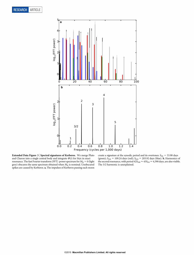
Extended Data Fig. 2 shows that Kerberos contributes to the chaos.To understand its role, we perform simulations in which Pluto andCharon have been merged into one central body, thereby isolating theeffects of the other moons on W. We perform integrations with MK 50 and with MK nominal, and then Fourier transform W(t) to detect thefrequencies of the perturbations (Extended Data Fig. 3). When MK isnon-zero, the power spectrum shows strong harmonics of the threesynodic periods SSK, SNK and SKH; this is because W(t) is a linearcombination of lS(t), lN(t) and lH(t), and Kerberos perturbs eachmoon during each passage. The harmonics of a second three-bodyresonance also appear: W9 5 42lS 2 85lN 1 43lK < 180u, that is,42SNK < 43SSN. This was the second strongest resonance found in oursearch; at the orbit of Styx, the two resonances are separated by just4 km. This is reminiscent of the Uranus system, where chains of near-resonances drive the chaos in that system13,14.
These results will influence future models of Pluto system forma-tion. Charon was probably formed by a large impact into Pluto15, andthe outer moons accreted from the leftover debris. If Charon had alarge initial eccentricity, then its corotation resonances could lockmaterial into the 1:3:4:5:6 relationship16. As Charon’s eccentricitydamped, the resonant strengths waned, but the moons were left withperiods close to these integer ratios17. This appealing model hasnumerous shortcomings, however18–20. The presence of a strong
Laplace-like resonance places a new constraint on formation models.Additionally, future models must account for the non-zero eccent-ricities and inclinations of the small satellites; for example, thesemight imply that the system was excited in the past by resonancesthat are no longer active21,22.
The resonance enforces a modified relationship between orbits: ifPN/PC 5 4 and PH/PC 5 6, then PS/PC 5 36/11 < 3.27. Nevertheless,the other three near-integer ratios remain unlikely to have arisen bychance. Excluding Styx, the probability that three real numbers wouldall fall within 0.11 of integers is just 1%.
Shapes, sizes and physical propertiesMean disk-integrated photometry for each moon is listed in Table 1.To infer the sizes of these bodies, we also require their visual geometricalbedos pv. Charon is a relatively bright, with pv < 0.38. Kuiper Beltobjects (KBOs) exhibit a large range of albedos, but the smallest KBOstend to be dark; pv < 0.04–0.08 is common23–26.
The photometry is expected to vary with phase angle a and, if abody is elongated or has albedo markings, with rotational phase.Extended Data Fig. 4 shows the raw photometry for Nix and Hydra.In spite of the otherwise large variations, an opposition surge is appar-ent for a 9 0.5u; this is often seen in phase curves and is indicativeof surface roughness. After dividing out the phase function model,Fig. 4 shows our measurements versus orbital longitude relative toEarth’s viewpoint. The measurements of Nix show no obviouspattern, suggesting that it is not in synchronous rotation; this is dis-cussed further below.
With unknown rotation states, we can only assess the light curves ina statistical sense. We proceeded with some simplifying assumptions.(1) Each moon is a uniform triaxial ellipsoid, with dimensions(a100, b100, c100), assuming pv 5 1. (2) Each measurement was takenat a randomly chosen, unknown rotational phase. (3) Each moon was
Elapsed time (years)0 2,000 4,000
360
180
0
180
0
180
0
a
b
c
(°)
Φ(°
)Φ
(°)
Φ
Figure 2 | Numerical integrations of the Styx–Nix–Hydra resonance.Resonant angle W is plotted versus time from the current epoch, usingthree assumptions for GMH: 0.0032 km2 s23 (a), 0.0039 km2 s23 (b), and0.0046 km2 s23 (c); these values are equivalent to the nominal mass, a 0.25sincrease, and a 0.5s increase6. GMN 5 0.0044 km2 s23 throughout, equivalentto 0.5s above its nominal mass. The modest increase in MH is sufficient to forcea transition of W from circulation (Styx outside resonance) to libration (Styxlocked in resonance).
Hydra GM (10–4 km3 s–2)
32 6030
58
Nix
GM
(10–4
km
3 s–2
)
44
46
Figure 3 | Mass-dependence of the Laplace-like resonance. The shade ofeach square indicates whether the associated pair of mass values producescirculation (black) or libration (white) during a 10,000-year integration.The moon masses MH and MN are each allowed to vary from nominal tonominal 1 1s (ref. 6). MK is nominal. Shades of grey define transitional states:light grey if W is primarily circulating; dark grey if W is primarily librating;medium grey for intermediate states. The transition between black and whiteis not monotonic, suggesting a fractal boundary.
4 J U N E 2 0 1 5 | V O L 5 2 2 | N A T U R E | 4 7
ARTICLE RESEARCH
G2015 Macmillan Publishers Limited. All rights reserved
in fixed rotation about its short axis. (4) The pole orientation may havechanged during the gap in coverage between years; this is consistentwith Supplementary Video 1, in which the rotation poles are generallystable for months at a time. We therefore describe the orientation bythree values of sub-Earth planetocentric latitude: w2010, w2011, and w2012.We used Bayesian analysis to solve for the six parameters that providethe best statistical description of the data; see the Methods sectionfor details.
Nix has an unusually large axial ratio of ,2:1 (Table 1), comparableto that of Saturn’s extremely elongated moon, Prometheus. Hydra isalso elongated, but probably less so. Also, Nix’s year-by-year varia-tions (Fig. 4) are the result of a rotation pole apparently turningtowards the line of sight; this explains both its brightening trendand also the decrease in its variations during 2010–2012 (ExtendedData Fig. 5). Pluto’s sub-Earth latitude is 46u, so Hydra’s measuredpole is nearly compatible with the system pole. Nix’s pole was ,20umisaligned in 2010 but may have reached alignment by 2012.
Given the inferred volume and an assumed albedo and density, wecan estimate GM, where M is the mass and G is the gravitation con-stant. We consider four assumptions about the moons’ physical prop-erties, and compare GM to the dynamical estimates6 (Table 1). Nixand Hydra are probably bright, Charon-like objects; if they weredarker, then GM would be too large to be compatible with upperlimits on the masses12.
Kerberos seems to be very different (Table 1). The dynamical infer-ence that its mass is about a third that of Nix and Hydra, yet that itreflects only ,5% as much sunlight, implies that it is very dark. Thisviolates our expectation that the moons should be self-similar dueto the ballistic exchange of regolith27. Such heterogeneity has oneprecedent in the Solar System: at Saturn, Aegaeon is very dark (pv
,0.15), unlike any other satellite interior to Titan, and even though itis embedded within the ice-rich G ring28. The formation of such aheterogeneous satellite system is difficult to understand.Alternatively, the discrepancy would go away if the estimate of MK
is found to be high by ,2s; this has a nominal likelihood of ,1%.Further study is needed.
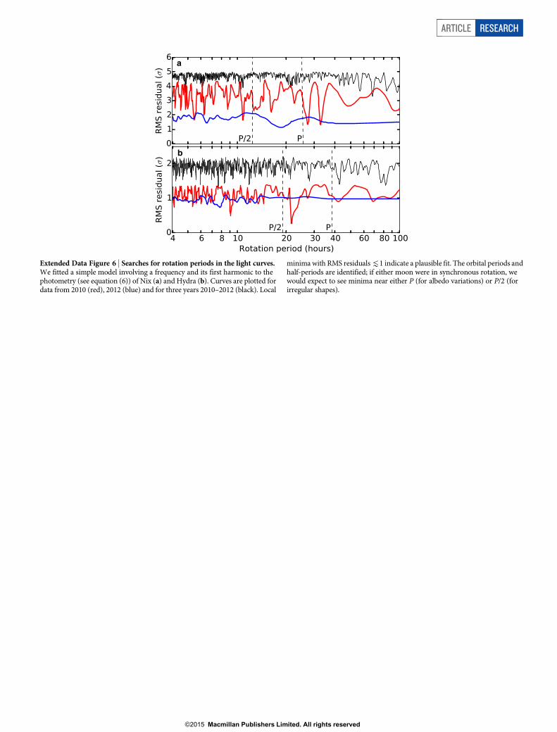
Rotation statesNearly every moon in the Solar System rotates synchronously; theonly confirmed exception is Hyperion, which is driven into chaoticrotation by a resonance with Titan29,30. Neptune’s highly eccentricmoon Nereid may also rotate chaotically31, but observational supportis lacking32,33. We have searched for rotation periods that are consist-ent with the light curves of Nix and Hydra (Fig. 4), but results havebeen negative (Extended Data Fig. 6). Although we can sometimesfind a rotation period that fits a single year’s data (spanning 2–6months), no single rotation period is compatible with all three yearsof data.
Dynamical simulations explain this peculiar result: a binary planettends to drive its moons into chaotic rotation. This is illustrated inFig. 5, showing the simulated rotation period and orientation of Nixversus time. The moon has a tendency to lock into near-synchronousrotation for brief periods, but these configurations do not persist.At other times, the moon rotates at a period entirely unrelated to its
a
b
Longitude with respect to Earth (°)–180 –90 0 90 180
450
500
550
600
650
700
Nor
mal
ized
pho
tom
etry
(km
2 )N
orm
aliz
ed p
hoto
met
ry (k
m2 )
300
350
400
450
500
550
Figure 4 | Normalized light curves. Disk-integrated photometry and 1s errorbars for Nix (a) and Hydra (b) have been normalized to a 5 1u and then plottedas a function of projected orbital longitude. Here 0u corresponds to inferiorconjunction with Pluto as seen from Earth. Measurements are colour-coded byyear: red for 2010, green for 2011, and blue for 2012. A tidally locked moonwould systematically brighten at maximum elongation (90u and 270u).
a
b
Time (days)
0 1,000 2,000
70
50
30
10
270
180
90
0
–90
Orie
ntat
ion
(°)
Per
iod
(day
s)
Figure 5 | Numerical simulations of Nix’s rotation. a, The instantaneousrotation period is compared to the synchronous rate (dashed line). b, Theorientation is described by the angle between Nix’s long axis and the direction
towards the barycentre. Nix librates about 0u or 180u for periods of time, but itjumps out of these states frequently.
4 8 | N A T U R E | V O L 5 2 2 | 4 J U N E 2 0 1 5
RESEARCH ARTICLE
G2015 Macmillan Publishers Limited. All rights reserved
orbit. Supplementary Video 1 provides further insights into the beha-viour; for example, it shows occasional pole flips, a phenomenonconsistent with the observed changes in Nix’s orientation.Lyapunov times are estimated to be a few months, or just a few multi-ples of the moons’ orbital periods. The timescale of the chaos dependson initial conditions and on assumptions about the axial ratios of themoons. The torques acting on a less-elongated body such as Hydra areweaker, but nevertheless our integrations support chaos.
According to integrations spanning a few centuries, a moon thatbegins in synchronous rotation will stay there, albeit with large libra-tions. It is therefore possible for synchronous rotation about Pluto andCharon to be stable. However, the large and regular torques of Plutoand Charon probably swamp the small effects of tidal dissipationwithin the moons, so they never have a pathway to synchronous lock.
Both photometry and dynamical models support the hypothesisthat Nix and Hydra are in chaotic rotation. The mechanism is similarto that driving Hyperion’s chaos, with Charon playing Titan’s role.However, Titan’s influence on Hyperion is magnified by a strongorbital resonance. For a binary such as Pluto–Charon, it appears tobe a general result that non-spherical moons may rotate chaotically;no resonance is required.
Future observationsThe New Horizons spacecraft will fly past Pluto on 14 July 2015. Atthat time, many of the questions raised by this paper will be addressed.Although Kerberos will not be well resolved (2–3 km per pixel),images will settle the question of whether it is darker than the othermoons. The albedos and shapes of Nix (imaged at 90.5 km per pixel)and Hydra (at 1 km per pixel) will be very well determined. NewHorizons will not obtain precise masses for the outer moons, butongoing Earth-based astrometry and dynamical modelling will con-tinue to refine these numbers, while also providing new constraints onthe Laplace-like resonance. Because this resonance has a predictedlibration period of centuries, the dynamical models will confirm orrefute it long before a complete libration or circulation period can beobserved.
Chaotic dynamics makes it less likely that we will find rings oradditional moons of Pluto. Within the Styx–Hydra region, the onlystable orbits are co-orbitals of the known moons. The region beyondHydra appears to be the region in which it is most likely that we willfind additional moons17, although some orbits close to Pluto are alsostable34. Independent of the new discoveries in store, we have alreadylearned that Pluto hosts a rich and complex dynamical environment,seemingly out of proportion to its diminutive size.
Online Content Methods, along with any additional Extended Data display itemsandSourceData, are available in the online version of the paper; references uniqueto these sections appear only in the online paper.
Received 29 October 2014; accepted 31 March 2015.
1. Showalter, M. R. et al. New satellite of (134340) Pluto: S/2011 (134340). IAU Circ.9221 (2011).
2. Weaver, H. et al. Discovery of two new satellites of Pluto. Nature 439, 943–945(2006).
3. Showalter, M. R. et al. New satellite of (134340) Pluto: S/2012 (134340). IAU Circ.9253 (2012).
4. Weaver, H. A. et al. New satellite of (134340) Pluto: S/2011 (134340). IAU Circ.9221 (2011).
5. Buie, M. W., Grundy, W. M. & Tholen, D. J. Astrometry and orbits of Nix, Kerberos,and Hydra. Astron. J. 146, 152 (2013).
6. Brozovic, M., Showalter, M. R., Jacobson, R. A. & Buie, M. W. The orbits and massesof satellites of Pluto. Icarus 246, 317–329 (2015).
7. Steffl, A. J. et al. New satellite of (134340) Pluto: S/2011 (134340). IAU Circ. 9221(2011).
8. Lee, M. H. & Peale, S. J. On the orbits and masses of the satellites of the Pluto-Charon system. Icarus 184, 573–583 (2006).
9. Buie, M. W. et al. Orbits and photometry of Pluto’s satellites: Charon, S/2005 P1,and S/2005 P2. Astron. J. 132, 290–298 (2006).
10. Sinclair, A. T. The orbital resonance amongst the Galilean satellites of Jupiter. Mon.Not. R. Astron. Soc. 171, 59–72 (1975).
11. Rivera, E. J.et al.The Lick-Carnegie ExoplanetSurvey: a Uranus-mass fourthplanetfor GJ 876 in an extrasolar Laplace configuration. Astrophys. J. 719, 890–899(2010).
12. Youdin, A. N., Kratter, K. M. & Kenyon, S. J. Circumbinary chaos: using Pluto’snewest moon to constrain the masses of Nix and Hydra. Astrophys. J. 755, 17(2012).
13. Quillen, A. C. & French, R. S. Resonant chains and three-body resonances in theclosely-packed inner Uranian satellite system. Mon. Not. R. Astron. Soc. 445,3959–3986 (2014).
14. French, R. G., Dawson, R. I. & Showalter, M. R. Resonances, chaos, and short-terminteractions among the inner Uranian satellites. Astron. J. 149, 142–169 (2015).
15. Canup, R. M. A giant impact origin of Pluto-Charon. Science 307, 546–550 (2005).16. Ward, W. R. & Canup, R. M. Forced resonant migration of Pluto’s outer satellites by
Charon. Science 313, 1107–1109 (2006).17. Kenyon, S. J.& Bromley,B. C. The formation of Pluto’s low-mass satellites. Astron. J.
147, 8–24 (2014).18. Lithwick, Y. & Wu, Y. The effect of Charon’s tidal damping on the orbits of Pluto’s
three moons. Preprint at http://arxiv.org/abs/0802.2939 (2008).19. Lithwick, Y. & Wu, Y. On the origin of Pluto’s minor moons, Nix and Hydra. Preprint
at http://arxiv.org/abs/0802.2951 (2008).20. Walsh, K. & Levison, H. F. Formation and evolution of Pluto’s small satellites.
Preprint at http://arxiv.org/abs/1505.01208 (2015).21. Zhang, K.& Hamilton,D.P.Orbital resonances in the innerNeptuniansystem I. The
2:1 Proteus-Larissa mean-motion resonance. Icarus 188, 386–399 (2007).22. Zhang, K. & Hamilton, D. P. Orbital resonances in the inner Neptunian system II.
Resonant history of Proteus, Larissa, Galatea, and Despina. Icarus 193, 267–282(2008).
23. Grundy, W. M., Noll, K. S. & Stephens, D. C. Diverse albedos of small trans-neptunian objects. Icarus 176, 184–191 (2005).
24. Lykawka, P. S. & Mukai, T. Higher albedos and size distribution of largetransneptunian objects. Planet. Space Sci. 53, 1319–1330 (2005).
25. Stansberry, J. et al. in The Solar System beyond Neptune (eds Barucci, M. A. et al.)161–179 (Univ. Arizona Press, 2007).
26. Lacerda, P. et al. The albedo–color diversity of transneptunian objects. Astrophys. J.793, L2 (2014).
27. Stern, S. A. Ejecta exchange and satellite color evolution in the Pluto system, withimplications for KBOs and asteroids with satellites. Icarus 199, 571–573 (2009).
28. Hedman, M. M., Burns, J. A., Thomas, P. C., Tiscareno, M. S. & Evans, M. W. Physicalproperties of the small moon Aegaeon (Saturn LIII). Eur. Planet. Space Congr. Abstr.6, 531 (2011).
29. Wisdom, J., Peale, S. J. & Mignard, F. The chaotic rotation of Hyperion. Icarus 58,137–152 (1984).
30. Klavetter, J. J. Rotation of Hyperion. I—Observations. Astron. J. 97, 570–579(1989).
31. Dobrovolskis, A. R. Chaotic rotation of Nereid? Icarus 118, 181–198 (1995).32. Buratti, B. J., Gougen, J. D. & Mosher, J. A. No large brightness variations on Nereid.
Icarus 126, 225–228 (1997).33. Grav, T., Holman, M. J. & Kavelaars, J. J. The short rotation period of Nereid.
Astrophys. J. 591, L71 (2003).34. Giuliatti Winter, S. M., Winter, O. C., Vieira Neto, E. & Sfair, R. Stable regions around
Pluto. Mon. Not. R. Astron. Soc. 430, 1892–1900 (2013).
Supplementary Information is available in the online version of the paper.
AcknowledgementsM.R.S. acknowledgesNASA’sOuterPlanetsResearchProgramfortheir support through grants NNX12AQ11G and NNX14AO40G. Support for HSTprogramme GO-12436 was provided by NASA through a grant from the SpaceTelescope Science Institute, which is operated by the Association of Universities forResearch in Astronomy, Inc., under NASA contract NAS5-26555. D.P.H. acknowledgesNASA Origins Research Program and grant NNX12AI80G.
Author Contributions M.R.S. performed all of the astrometry, photometry, orbit fittingand numerical modelling discussed here. D.P.H. was co-investigator on the Kerberosdiscovery and has participated in the dynamical interpretations of all the results.
Author Information Reprints and permissions information is available atwww.nature.com/reprints. The authors declare no competing financial interests.Readers are welcome to comment on the online version of the paper. Correspondenceand requests for materials should be addressed to M.R.S. ([email protected]).
4 J U N E 2 0 1 5 | V O L 5 2 2 | N A T U R E | 4 9
ARTICLE RESEARCH
G2015 Macmillan Publishers Limited. All rights reserved
METHODSData selection and processing. Our data set encompasses all available HSTimages of the Pluto system during 2006 and 2010–2012, plus Kerberos in 2005.We neglected HST observations from 2002, 2003, and 20075,10, because they are ofgenerally lower quality, rendering Kerberos and Styx undetectable. We empha-sized long exposures through broad-band filters, although brief exposures ofCharon and Pluto provided geometric reference points. Supplementary Table 1lists the images and bodies measured. We analysed the calibrated (‘flt’) image files.To detect Kerberos and Styx, it was often necessary to align and co-add multipleimages from the same visit; files produced in this manner are listed in the tablewith a ‘coadd’ suffix.
We fitted a model point spread function (PSF) to each detectable body. ThePSFs were generated using the ‘Tiny Tim’ software maintained by the SpaceTelescope Science Institute (STScI)35,36. Upon fitting to the image, the centre ofthe PSF provides the astrometry and the integrated volume under the two-dimen-sional curve, minus any background offset, is proportional to the disk-integratedphotometry. We measured objects in order of decreasing brightness and sub-tracted each PSF before proceeding; this reduced the effects of glare on fainterobjects. Measurements with implausible photometry were rejected; this was gen-erally the result of nearby background stars, cosmic ray hits, or other image flaws.Further details of the analysis are provided elsewhere6. Styx photometry (Table 1)might be biased slightly upward by our exclusion of non-detections; however,photometry of the other moons is very robust.The Pluto–Charon gravity field. We have simplified the central gravity field bytaking its time-average. The resulting cylindrically symmetric gravity field canthen be expressed using the same expansion in spherical harmonics that is tra-ditionally employed to describe the field of an oblate planet:
V r, h, wð Þ~{GM=r 1{X?
m~2
Jm R=rð ÞmPm sin wð Þ" #
ð1Þ
Here (r, h, w) are polar coordinates, where r is radius and h and w are longitudeand latitude angles, respectively; G is the gravitation constant, M is the body’smass, R is its equatorial radius, Pm is the mth Legendre polynomial, Jm is the mthcoefficient in the expansion. The dependence on h and the odd m-terms in theseries vanish by symmetry. The coefficients Jm can be determined by noting thatthe potential along the axis of the ring simplifies considerably:
V r, w~p=2ð Þ~{GM=r 1z R=rð Þ2# ${1=2 ð2Þ
This can then be compared to the definition of Legendre polynomials:
1{2xtzt2! "{1=2~X?
m~0
tmPm xð Þ ð3Þ
Substituting t 5 (R/r) and evaluating the expression for x 5 0 yields:
V r, w~p=2ð Þ~{GM=rX?
m~0
R=rð ÞmPm 0ð Þ ð4Þ
Noting that Pm(1) 5 1 for all m, equations (1) and (4) can only be equal if thecoefficients Jm are negatives of the Legendre polynomials evaluated at zero: J2 51/2, J4 5 23/8, J6 5 5/16, and so on. Given this sequence of coefficients, we candetermine n, _$ and _V as functions of semimajor axis a:
n2 að Þ~GM=a3 1{X?
m~2
1zmð ÞJm R=að ÞmPm 0ð Þ
" #
ð5aÞ
k2 að Þ~GM=a3 1{X?
m~2
ð1{m2ÞJmðR=aÞmPm 0ð Þ" #
ð5bÞ
v2 að Þ~GM=a3 1{X?
m~2
1zmð Þ2Jm R=að ÞmPm 0ð Þ" #
ð5cÞ
Here k is the epicyclic frequency and _n is the vertical oscillation frequency. Itfollows that _$ að Þ~n að Þ{k að Þ and _V að Þ~n að Þ{v að Þ. In practice, we treated nas the independent variable because it has the strictest observational constraints,and then derived a, _$ and _V from it.Orbit fitting. We modelled each orbit as a Keplerian ellipse in the P–C frame, butwith additional terms to allow for apsidal precession and nodal regression. Ourmodel is accurate to first order in e and i; any second-order effects can beneglected because they would be minuscule compared to the precision of ourmeasurements.
We also required an estimate for the location of the system barycentre in each setof images. Because HST tracking is extremely precise between consecutive images,the barycentre location was only calculated once per HST orbit. We solved for thebarycentre locations first and then held them fixed for subsequent modelling of theorbital elements. Barycentre locations were derived from the astrometry of Pluto,Charon, Nix and Hydra. We locked Pluto and Charon to the latest ephemerisdistributed by the Jet Propulsion Laboratory, PLU0436. We accounted for the offsetbetween the centre of light and centre of body for Pluto using the latest albedo map37.However, because the number of Pluto and Charon measurements is limited, wealso allowed Nix and Hydra to contribute to the solution. For each single year 2006–2012, we solved simultaneously for the barycentre location in each image set and alsofor orbital elements of Nix and Hydra. For the detection of Kerberos in 2005, theonly available pointing reference was Hydra, which we derived from PLU043. Byallowing many measurements to contribute to our barycentre determinations, wecould improve their quality but also limit any bias introduced by shortcomings ofour orbit models. The derived uncertainties in the barycentre locations are muchsmaller than any remaining sources of error.
A nonlinear least-squares fitter identified the best value for each orbital ele-ment and also the covariance matrix, from which uncertainties could be derived.However, as noted in Table 1 and Extended Data Table 1, our RMS residuals(equivalent to the square root of x2 per degree of freedom) exceed unity. For Styxand Kerberos, marginal detections probably contributed to the excess; for Nix andHydra, we have identified the source as the un-modelled wobbles in the orbits. Alluncertainty estimates have been scaled upward to accommodate these under-estimates.
During the orbit fits, we rejected individual points with excessive residuals,based on the assumption that they were misidentifications or the results of poorPSF fits. Extended Data Table 1 lists values for the number of included (M1) andrejected (M0) measurements. Rejecting points, however, would bias our uncer-tainty estimates downward. We compensated by running Monte Carlo simula-tions in which we generated (M0 1 M1) Gaussian distributed, two-dimensionalrandom variables and then rejected the M0 that fall furthest from the origin. Thestandard deviation among the remainder then gave us an estimate of the factor bywhich we might have inadvertently reduced our error bars. With this procedure,accidentally rejecting a small number of valid measurements would not bias theuncertainties.
We also explored the implications of making various assumptions about howthe orbital elements are coupled (Extended Data Table 1). For the purposes of thispaper, we have adopted the N 5 8 solutions in which _V can be derived from n and_$. This assumption is helpful because, when e and i are small, the frequencies _$
and _V are especially difficult to measure. By allowing them to be coupled, weobtained more robust results. Nevertheless, our expectation that _$ and _V shouldbe roughly equal in magnitude but opposite in sign has been well supported bymost of our uncoupled, N 5 9 fits.Resonance analysis. We have defined a general resonance using a set of integercoefficients (pj, qj, rj). The strength of a resonance is equal to C(p, q, r)PmjPej
jqjj
Psinjrjj(ij), where mj is the mass ratio of moon j to the mass of Pluto. The firstproduct Pmj excludes the mass of the smallest moon involved, because a resonancecan exist even if one moon is a massless test particle. The function C defines astrength factor, but because it has no simple expression, we ignore it in this analysisexcept to note, qualitatively, that the strongest resonances tend to involve smallcoefficients and/or small differences between coefficients.
We performed an exhaustive search for all possible resonances involving up tofour non-zero coefficients, with jpjj # 300, jqjj # 4, and jrjj # 4. Symmetrydictates that the coefficients sum to zero and that
Pj
rj must be even38. Because
Charon follows a circular, equatorial orbit, qC 5 rC 5 0. We first identified
possible resonances by _Wv0:1u per day, and then followed up by evaluating Wfor each year. Sets of coefficients for which W values clustered near 0u or 180uweregiven preference. We also favoured sets of coefficients that have simple physicalinterpretations, and where the absolute values were small and/or close to oneanother.Orbital integrations. Our orbit simulations employed the numeric integratorSWIFT39,40. We used PLU0436 as our reference ephemeris; it provides state vec-tors (positions and velocities) for all the bodies in the system versus time. Forsimplicity, we neglected bodies outside the Pluto system in most integrations. TheSun is the dominant external perturber, shifting the moons by a few tens ofkilometres, primarily in longitude, after one Pluto orbit of 248 years; this is,1% of our orbital uncertainties.
Each integration must begin with initial state vectors and masses for each body.However, the state vectors and masses are closely coupled; any change to onemass requires that we adjust all of the state vectors in order to match the observedorbits. Ideally, this would be accomplished by re-fitting to all of the available
RESEARCH ARTICLE
G2015 Macmillan Publishers Limited. All rights reserved
astrometry, but that task is beyond the scope of this paper. To simplify theproblem, we generated false astrometry derived directly from PLU043, butsampled at the times of all prior HST visits that detected one or more of the fourouter moons. Such measurements date back to 11 June 20025,6,9. For each set ofassumed masses, we used a nonlinear least-squares fitter to solve for the initialstate vectors that optimally matched this astrometry. A similar technique wasused to model the effects of moon masses on the chaotic dynamics of the Uranussystem41. This procedure guarantees that our numeric integrations will match theactual astrometry with reasonable accuracy, regardless of the masses assumed.
For a few numerical experiments, we investigated the consequences of placingStyx exactly into its Laplace-like resonance (Extended Data Figs 2 and 3). Weaccomplished this by generating a different set of false astrometry, in which theposition of Styx was derived from the requirement that W 5 180u at all times.Photometry. Our numerical simulations suggest that typical rotation periods foreach moon are comparable to the orbital period, that is, several weeks. Becausethis timescale is long compared to one or a few of HST’s 95-min orbits, wecombined measurements obtained from single or adjacent orbits. InSupplementary Table 1, adjacent orbits are indicated by an orbit number of 2or 3. Our photometry (Fig. 4 and Extended Data Fig. 4) is defined by the mean andstandard deviation of all measurements from a single set of orbits.
We considered two simple models for the light curves described as reflectivityA versus time t:
A1 tð Þ~c0zc1 sin vtð Þzc2 cos vtð Þ ð6aÞ
A2 tð Þ~c0zc1 sin vtð Þzc2 cos vtð Þzc3 sin 2vtð Þzc4 cos 2vtð Þ ð6bÞ
We then sought the frequency v that minimizes residuals. Given the small num-ber of measurements in individual years, it was inappropriate to attempt moresophisticated models. Results are shown in Extended Data Fig. 6. For the datafrom 2010, we did identify frequencies where the residuals are especially small,suggesting that we may have identified a rotation rate for that subset of the data.However, in no case does a frequency persist from 2010 to 2012.Shape modelling. We have described the axial orientation relative to the line ofsight using sub-Earth planetocentric latitude w. The hypothetical light curveof an ellipsoid is roughly sinusoidal; its projected cross-section on the skyvaries between extremes Amin and Amax. If w 5 0, Amin 5 pbc and Amax 5 pac.If w 5 90u, then Amin 5 Amax 5 pab. More generally
Amin a,b,c,wð Þ~pb c2 cos2 wza2 sin2 w! "1=2 ð7aÞ
Amax a,b,c,wð Þ~pa c2 cos2 wzb2 sin2 w! "1=2 ð7bÞ
If w is fixed and each measurement was obtained at a uniformly distributed,random rotational phase, then the conditional probability density function fora cross-section A given Amin and Amax is:
P AjAmin, Amaxð Þ! 1{ A{A0ð Þ=DA½ $2! "{1=2 ð8Þ
where A0 ; (Amax 1 Amin)/2 and DA 5 (Amax 2 Amin)/2. In reality, eachmeasurement A has an associated uncertainty s. This has the effect of convolvingP with a normal distribution N(A, s), with zero mean and standard deviation s.
where the fl operator represents convolution.However, simulations show that w varies due to chaotic rotation driven by the
central binary (Supplementary Video 1). To simplify this analysis, we haveassumed that w was fixed for the whole of each year during which we obtaineddata, but that changes may have occurred between years; this is generally con-sistent with the time spans of our data sets (a few months per year) and theinfrequency of large pole changes in the simulations. This leads us to define threeunknowns: w2010, w2011, and w2012. Because Amin and Amax depend only on sin2wand cos2w, we replace the unknowns w by S ; sin2w in our analysis.
We have a vector of independent measurements A 5 (A0, A1, ….) and uncer-tainties s 5 (s0, s1,….), so the joint, conditional probability of obtaining all ourmeasurements is a product:
P Aja, b, c, S2010, S2011, S2012ð Þ
~ PP sk½ $ AkjAmin a, b, c, Syear kð Þ! "
, Amax a, b, c, Syear kð Þ! "! " ð10Þ
where year(k) is the year associated with measurement k. Instead, we seek thejoint, conditional probability density function P(a, b, c, S2010, S2011, S2012jA). Thisis a problem in Bayesian analysis:
P a, b, c, S2010, S2011, S2012jAð Þ
~ P Aja, b, c, S2010, S2011, S2012ð ÞP Að Þ=P a, b, c, S2010, S2011, S2012ð Þð11Þ
Here P(A) and P(a, b, c, S2010, S2011, S2012) represent our assumed ‘prior prob-ability’ distributions for these quantities. We have no prior information about ourmeasurements Ak, so we assume that they are uniformly distributed. The secondprior can be broken down as
P a, b, c, S2010, S2011, S2012ð Þ~P a, b, cð ÞP S2010ð ÞP S2011ð ÞP S2012ð Þ ð12Þ
because orientations are independent of shape and of one another. If the polein each year is randomly distributed over 4p steradians, then P(w)/ cos w andP(S) / S21/2.
We model our prior for the shape as P(a, b, c) 5 P1(u)P2(v)P3(w), where u ;abc; v ; a/b; and w ; b/c. This states that we will regard the ellipsoid’s volume andits two axial ratios as statistically independent. We have assumed that log(u) isuniformly distributed rather than u itself, which implies P1(u) / 1/u. Experiencewith other irregularly shaped planetary objects suggests that large ratios a/b andb/c are disfavoured, with values rarely exceeding 2. After some experimentation,we adopted P2(v) / 1/v3 and P3(w) / 1/w3. Alternative but similar assumptionshad little effect on our results.
The above equations provide a complete solution to the joint probability func-tion P(a, b, c, S2010, S2011, S2012). We solved for the complete six-dimensionalfunction, represented as a six-dimensional array. Quantities listed in Table 1 werederived as the mean and standard deviation of P along each of its six axes, with Sconverted back to w. Extended Data Fig. 5 compares the distribution of measure-ments by year with the reconstructed probability distributions.Simulations of rigid body rotation. The orientation of the ellipsoid can be definedby a unit quaternion: q 5 [cos(h/2), sin(h/2)u] represents a rotation by angle habout unit axis vector u. The time-derivative dq/dt 5 [0, v]?q/2, where v is thespin vector. We used a Bulirsch–Stoer integrator to track q, dq/dt, x and dx/dt,where x is the position of the ellipsoid relative to the barycentre. Theforces and torques acting were defined by Pluto and Charon followingfixed circular paths around the barycentre; this motion was pre-defined forthe simulations, not integrated numerically. We derived d2x/dt2 from thegravity force of each body on the ellipsoid. We also required thesecond derivative of q: d2q/dt2 5 [2jvj2/2, a]?q/2, where a is the time-derivative of v. We related a to the torque applied by Pluto and Charonon the ellipsoid
t~3GMPrP| IrPð Þ%
rPj j5z3GMCrC| IrCð Þ%
rCj j5 ð13Þ
where rk 5 x 2 xk is the vector offset from each body centre to the ellipsoid’scentre and I is the ellipsoid’s moment of inertia tensor. In the internalframe of the ellipsoid, the moment of inertia tensor I0 is diagonal, withI11 5 (M/5)(b2 1 c2), I22 5 (M/5)(a2 1 c2), and I33 5 (M/5)(a2 1 b2). Itis rotated to the system coordinate frame via the rotation matrix R, which canbe calculated from q: I 5 RI0RT. We then solve for a via the relation t 5 Ia1 v 3 Iv.Code availability. Portions of our software are available at https://github.com/seti/pds-tools. We have opted not to release the entire source code because it isbuilt on top of additional large libraries representing decades of development.Instead, we have documented our algorithms with sufficient detail to enableothers to reproduce our results.
35. Krist, J. E., Hook, R. N. & Stoehr, F. 20 years of Hubble Space Telescope opticalmodeling using Tiny Tim. Proc. SPIE 8127, 1–16 (2011).
36. Space Telescope Science Institute. Observatory Support: Tiny Tim HST PSFModeling http://www.stsci.edu/hst/observatory/focus/TinyTim (2011).
37. Buie, M. W. et al. Pluto and Charon with the Hubble Space Telescope. II. Resolvingchanges on Pluto’s surface and a map for Charon. Astron. J. 139, 1128–1143(2010).
38. Hamilton, D. P. A comparison of Lorentz, planetary gravitational, and satellitegravitational resonances. Icarus 109, 221–240 (1994).
39. Levison, H. F. & Duncan, M. J. The long-term dynamical behavior of short-periodcomets. Icarus 108, 18–36 (1994).
40. Levison, H. F. SWIFT: A Solar System Integration Software Package http://www.boulder.swri.edu/,hal/swift.html (2014).
41. French, R. S. & Showalter, M. R. Cupid is doomed: An analysis of the stability of theinner Uranian satellites. Icarus 220, 911–921 (2012).
ARTICLE RESEARCH
G2015 Macmillan Publishers Limited. All rights reserved
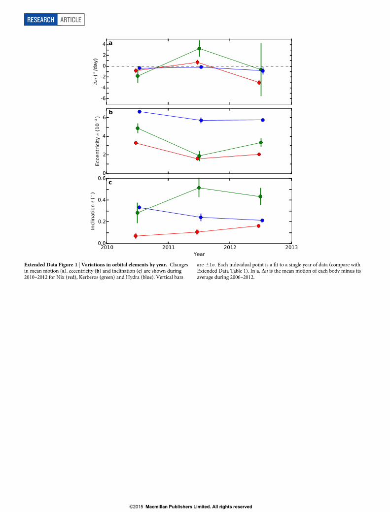
Extended Data Figure 1 | Variations in orbital elements by year. Changesin mean motion (a), eccentricity (b) and inclination (c) are shown during2010–2012 for Nix (red), Kerberos (green) and Hydra (blue). Vertical bars
are 61s. Each individual point is a fit to a single year of data (compare withExtended Data Table 1). In a, Dn is the mean motion of each body minus itsaverage during 2006–2012.
RESEARCH ARTICLE
G2015 Macmillan Publishers Limited. All rights reserved
Extended Data Figure 2 | The role of Kerberos in the Laplace-likeresonance. We have initiated an integration with Styx exactly in its resonancewith Nix and Hydra, and then have allowed it to evolve for 10,000 years. The
diagrams are for MK nominal (a), MK reduced by 1s (b) and MK 5 0 (c). Theamplitude of the libration is stable when Kerberos is massless, but shows erraticvariations otherwise.
ARTICLE RESEARCH
G2015 Macmillan Publishers Limited. All rights reserved
a
b
Extended Data Figure 3 | Spectral signatures of Kerberos. We merge Plutoand Charon into a single central body and integrate W(t) for Styx in exactresonance. The fast Fourier transform (FFT) power spectrum for MK 5 0 (lightgrey) obscures the same spectrum obtained when MK is nominal. Unobscuredspikes are caused by Kerberos. a, The impulses of Kerberos passing each moon
create a signature at the synodic period and its overtones: SSK 5 53.98 days(green); SNK 5 109.24 days (red); SKH 5 203.92 days (blue). b, Harmonics ofthe second resonance, with period 42SNK < 43SSN < 4,590 days, are also visible.The 3/2 harmonic is unexplained.
RESEARCH ARTICLE
G2015 Macmillan Publishers Limited. All rights reserved
a
b
Extended Data Figure 4 | Satellite phase curves. Raw disk-integratedphotometry has been plotted versus phase angle a for Nix (a) and Hydra(b). Vertical bars are 61s. An opposition surge is apparent. A simpleparametric model for the phase curve is shown: c(1 1 d/a), where d is fixed but cis scaled to fit each moon during each year. Measurements and curves arecolour-coded by year: red for 2010, green for 2011, and blue for 2012.
ARTICLE RESEARCH
G2015 Macmillan Publishers Limited. All rights reserved
a
b
c
d
e
f
Extended Data Figure 5 | Distribution of photometric measurements byyear. The black curves show the theoretical probability density function (PDF)of A by year for Nix (a, 2010; b, 2011; c, 2012) and Hydra (d, 2010; e, 2011;f, 2012), after convolution with the measurement uncertainties. The histogram
of measurements from each year is shown in red. In spite of small numberstatistics, the measurements appear to be well described by the models, whichhave been derived via Bayesian analysis.
RESEARCH ARTICLE
G2015 Macmillan Publishers Limited. All rights reserved
a
b
Extended Data Figure 6 | Searches for rotation periods in the light curves.We fitted a simple model involving a frequency and its first harmonic to thephotometry (see equation (6)) of Nix (a) and Hydra (b). Curves are plotted fordata from 2010 (red), 2012 (blue) and for three years 2010–2012 (black). Local
minima with RMS residuals91 indicate a plausible fit. The orbital periods andhalf-periods are identified; if either moon were in synchronous rotation, wewould expect to see minima near either P (for albedo variations) or P/2 (forirregular shapes).
ARTICLE RESEARCH
G2015 Macmillan Publishers Limited. All rights reserved
Extended Data Table 1 | Orbital elements based on coupling various orbital elements and based on subsets of the data.
Columns M1 and M0 identify the numbers of measurements included in and excluded from the fit; N indicates the number of free parameters. When N 5 8, we derived _V from the relationship n2 5 2n2 2 k2. For N 5
7, _$ and _V were both derived from n and the gravity field using equations (5b) and (5c). For N 5 6, a was also coupled to n via equation (5a). N 5 3 indicates a fit to a circular orbit. For fits to single years of data, theepoch is 1 July UTC for that year. We disfavour N # 7 in the multi-year fits because some residuals increase markedly.
RESEARCH ARTICLE
G2015 Macmillan Publishers Limited. All rights reserved


![u c ^ h d m f g l r k l h c k k k b b N h j m f Z H j ] Z ... · PDF file... h \ u c ^ h d m f _ g l r _ k l h c k _ k k b b N h j m f Z H j ] Z g b a Z p b b H [ t _ ^ b g _ g g u](https://static.documents.pub/doc/80x56/5aae1c697f8b9a22118b9631/u-c-h-d-m-f-g-l-r-k-l-h-c-k-k-k-b-b-n-h-j-m-f-z-h-j-z-h-u-c-h-d.jpg)


![bonegraft rusça dental katalog · J k c [ h [ f c b ` l h c g e i ] ] c _ h i r m i i \ k [ b ` q c g ` ` m j i k c l m n y l m k n e m n k n c _ [ h h [ z l m k n e m n k [](https://static.documents.pub/doc/80x56/5e4035a47d2a7905ba60ca3f/bonegraft-rusa-dental-katalog-j-k-c-h-f-c-b-l-h-c-g-e-i-c-h-i-r-m.jpg)
