articol2 portfolio

8/12/2019 articol2 portfolio

http://slidepdf.com/reader/full/articol2-portfolio 1/17

T h e R e v i e w o f F i n a n c e a n d B a n k i n gVo lume 0 4 , Issue 1 , Yea r 2 0 1 2 , Pa g es 0 1 5 — 0 3 1S print ISSN 2 0 6 7 -2 7 1 3 , o nline ISSN 2 0 6 7 -3 8 2 5

ACTIVE PORTFOLIO MANAGEMENT IN THE PRESENCE OF REGIME

SWITCHING: WHAT ARE THE BENEFITS OF DEFENSIVE ASSET

ALLOCATION STRATEGIES IF THE INVESTOR FACES BEAR

MARKETS?

KLAUS GROBYS

Abstract. This paper studies the asset allocation decision in the presence of regime switch-ing in stock market returns. The analysis is based on two stock indices: DJI 30 and OMX30. The two-step optimization procedure employed points towards the usage of defensiveasset allocation strategies under bear markets and ordinary index tracking strategies underbull markets. The out-of-sample experiments strengthen the performance of active strategiesthat distinguish between diff erent regimes. Moreover, the Sharpe ratios of portfolios based

on such strategies are higher than the ones of ordinary index tracking based portfolios.

1. INTRODUCTION AND LITERATURE REVIEW

The portfolio selection process has become an important issue of modern portfolio man-agement. The traditional stock selection in prior related studies involves the optimizationprocedure in a mean-variance framework. Based on the seminal work of Markowitz (1959),Sharpe (1964), Black (1972) and Black and Litterman (1992) proposed a means of estimatingexpected asset returns to obtain better-behaved portfolio models. The Black and Litterman(1992) model, which is often referred to as active strategy, optimizes expected stock returns ina mean-variance framework, constructing a portfolio in which bets are taken only on stocks for

which the portfolio management has opinions on future expected returns. Thereby, the mag-nitude of bets in relation to the equilibrium portfolio weights depends on the confidence levelsspecified by the management and on a parameter specifying the weight of the collected investorbeliefs in relation to the market equilibrium, the weight-on-views. The Black and Litterman(1992) portfolio optimization model is widely applied, discussed and refined in the literature,as in studies by Chow (1995), Jones et al. (2007), Martellini and Ziemann (2007). However,Phengpis and Swanson (2011) argue that the magnitude of suggested gains that can be real-ized after portfolio formation is questionable, as the historically optimized portfolio tends toperform poorly out-of-sample due to the estimation error. In particular, the stocks that haveperformed well tend to be overweighted in the historically optimized portfolio. Other portfoliooptimization procedures, which focus mainly on tracking indices, are often referred to as passivestrategies. In particular, optimized sampling as suggested by van Montfort, Visser and Fijnvan Draat (2008) aims to find the portfolio that has tracked the underlying index as much as

possible in the past, hoping it will track the index the same way in future periods.According to Alexander (1999) and Alexander and Dimitriu (2005a), correlation based port-

folios can be very sensitive to the presence of outliers, non-stationarity or volatility clustering.

Received by the editors October 19, 2011. Accepted by the editors March 6, 2012.Keywords : Regime switching, Multiple asset allocation, Optimization, Maximum-Likelihood, Stock markets.JEL Classi fi cation : G12, G11, C32.Klaus Grobys, Ph.D., is Research Director at Swedish Research Association of Financial Economics, Hajom,

Sweden. E-mail: [email protected] paper is in final form and no version of it will be submitted for publication elsewhere.

c°2 0 1 2 T h e R e v i e w o f F i n a n c e a n d B a n k i n g

15



16 KLAUS GROB YS

Hence, they consider portfolio optimization procedures which are based on cointegration analy-sis. The cointegration approach to portfolio modeling allows for using the entire informationset in a system of stock prices. According to Granger and Terasvirta (1993) stock prices are

long-memory processes and therefore, cointegration can explain their long-run behavior. Friesenet al. (2009) argue that there is convincing evidence that stock prices display short-term mo-mentum over periods of six to twelve months involving mean reversion, as already suggestedin studies by De Bondt and Thaler (1985), Chopra et al. (1992) and Jegadeesh and Titman(1993). In contrast to correlation analysis, optimization procedures based on cointegrationanalysis aim at tracking the stochastic trends cached in the stock prices. Overall, this line of research outperforms its counterpart based on correlation analysis. Studies that investigate theperformance of portfolio optimization procedures based on cointegration analysis can be foundin Alexander and Dimitriu (2005a, b), Grobys (2010) and Phengpis and Swanson (2011).

Even though Alexander and Dimitriu (2005b) conclude that the entire abnormal return of acointegration based trading strategy is associated with the high volatility regime, their studydoes not account for an actively selected defensive strategy in such stock market crashes. Butwhat is the advantage of taking actively defensive positions when the investor faces a persistent

price bust, respectively, stock market crash? Extreme positions in stocks are basically associatedwith higher trading costs, but may it be that lowered losses induced by defensive positionsovercome the potentially higher trading costs1 aforementioned? Boldin and Cici (2010) showthat less than half of the actively managed equity funds outperform the average S&P 500 indexfund, which suggests that more importance should be given to strategically timing the market.

Guidolin and Timmermann (2008) see mounting empirical evidence that asset returns donot follow linear processes with stable coefficients, but a more complicated process involvingdiff erent regimes which are associated with individual return distributions. The latter is alsosupported by studies of Ang and Bekaert (2002a, b), Ang and Chen (2002), Guidolin andTimmermann (2005a, b, 2006a, b, c), Perez-Quiros and Timmermann (2001) and Whitelaw(2001). Typically observed regimes in stock markets are often referred to as bull- and bearmarkets or, in statistical terms, as low frequency trends which switch between persistent periodsexhibiting positive or negative returns on expectation. Traditional methods which are employed

in order to identify these trends rest typically upon an ex post assessment of the stock markets’peaks and troughs. Gonzalez et al. (2005), Lunde and Timmermann (2004) and Pagan andSossounov (2003) provide such dating algorithms involving a set of rules for classification. Theseapproaches have in common that a turning point can only be figured out several observationsafter it had occurred. Furthermore, the latent nature of low frequency trends is not accountedfor in any of these methodologies. Thus, they do not allow for statistical inference. Probabilitymodels which can be employed for statistical inference in the presence of low frequency trends arethe Markov-Switching (MS) models for which transitions between states, respectively, regimesare governed by a discrete parameter Markov chain (Guidolin and Timmermann, 2008, Grobys2011).

Ang and Bekaert (2002a) introduce regime switching into a dynamic international assetallocation setting. Thereby, they investigate a U.S. investor with constant relative risk aversionmaximizing the expected end-of-period utility and dynamically rebalancing the portfolio. Whileestimating regime-switching models on U.S., U.K., and German equity, their findings giveevidence of a high-volatility, high-correlation regime which tends to coincide with a bear market.The main result of the study is that the high volatility regime mostly induces a switch towardthe lower volatility assets, which are cash (if available), U.S. equity, and also German equity,if available. The statistical model employed by Ang and Bekaert (2002a) is a two-state regime

1If a portfolio manager takes extreme positions in stocks to take advantage of momentum eff ects, the positionshave to be changed, respectively, rebalanced more frequently in comparison to a portfolio that is constructed forordinary index replication, only. This may be a matter of the momentum eff ects, as the latter can be seen asstochastic short-run movements requiring highly frequented rebalancing and, as a consequence, higher tradingcosts (see also section “Discussion of the Results”).



A CT IV E P O RT FO L IO M A NA GE M EN T I N T HE P R ES EN C E O F R E GI ME S W IT CH IN G 1 7

switching model in which the states are assumed to be observable as mentioned by Guidolinand Timmermann (2008).

Guidolin and Timmermann (2008) study the asset allocation decision in the presence of

regime switching in asset returns and their model involves four states: crash, slow growth, bulland recovery. In contrast to Ang and Bekaert (2002a), Guidolin and Timmermann (2008) andGrobys (2011) treat the regime switching variable as unobservable. Guidolin and Timmermann(2008) investigate the optimal asset allocation of an US investor between bonds, stocks and cash.Against Barberis’ (2000) suggestion that the weight on stocks should increase as a function of the investor’s horizon, Guidolin and Timmermann (2008) find that this is no longer the casewhen change in regimes may occur, as the weight on stocks increases in the investment horizononly when investor faces the crash state at the time when the investment decision is made.Against this, the optimal allocation to stocks declines as a function of the investment horizonwhen the investors face a bull market, slow growth or recovery state. However, Guidolin andTimmermann (2008) underline that investors are supposed to adjust their portfolio weights asnew information arrives.

This contribution takes the presence of stock market regimes as a starting point and proceeds

to characterizing asset allocation implications for the equity portfolio management. The mod-eling approach can be divided in two parts: in the first step, the current stock market regime isestimated and this approach is closely related to Ang and Bekaert (2002a, b) and in particularGuidolin and Timmermann (2008) and Grobys (2011). The second step presents the optimiza-tion procedure which is dependent on the current regime. Thereby, the cointegration approachin accordance to Alexander (1999) and Alexander and Dimitriu (2005a, b) is employed in orderto exploit stock markets’ short-term momentum. There are no studies available that take intoaccount both features at the same time, namely a multiple asset allocation procedure embeddedin a two-step approach whereby the optimization procedure is dependent on the current stateof the system. This contribution which belongs to the literature of active portfolio managementremedies this current gap.

The next section provides an overview about the statistical methodology including statisticaltests to assess the model selection. Afterwards, the results of the study are discussed. The last

section concludes and identifies possible areas of future research.

2. ECONOMETRIC METHODOLOGY

The section describes a multiple asset allocation strategy with portfolios that aim at trackingthe underlying stock indices. Two strategies will be compared with each other. The firststrategy will be referred to as ordinary index-tracking strategy and considered as a passiveasset allocation strategy where the tracking-portfolio will be rebalanced regularly, irrespectiveif the investor faces a bull- or bear-market. The second strategy will be referred to as defensivestrategy and considered as an active asset allocation strategy where the tracked index switchesbetween the ordinary index and an artificial index. The latter will be referred to as defensiveindex. In doing so, the current regime can either be a bull-market where the investor expectspositive returns in the middle-run, or a bear-market where negative returns are expected.

Following Guidolin and Timmermann (2008), it will be supposed that the stock markets’mean and covariances in returns are driven by a common state variable, , that takes integervalues 1 :

= +

X=1

· − + (1)

⎛⎜⎝

1...

⎞⎟⎠ =

⎛⎜⎝

1 ...

⎞⎟⎠+

X=1

⎛⎜⎝

1−...

−

⎞⎟⎠+

⎛⎜⎝

1...

⎞⎟⎠ (2)



18 KLAUS GROB YS

In equation (1)

denotes the expectation of the respective stock-market and denotes thecorresponding stock-market return at time where the index = 1 indicates a monthlyfrequency series of log-returns. The parameters 1 and the mean

depend on the

current state . In Equation (2), ( 1 )0

is the expectation of the vector of returns(1 )

0

and it is state-dependent. Furthermore, (1 )0

¡ (0P

)where

denotes the number of stock markets. If = 10, equation (1) will be in line with Guidolin andTimmermann (2008) simplified to a standard vector-autoregression.

In the following, regime switching in the state variable (i.e. from“bear market” to “bullmarket” for instance) is governed by the transition probability matrix that is a 2matrixwith elements

( = | −1 = ) = = 1 (3)

where denotes the number of states that are accounted for. For = 2the transitionprobability matrix is

=µ 11 21

12 22¶

=µ 11 1 − 22

1 − 11 22¶

= ( ) (4)

Hence, each regime is the realization of a first-order Markov chain with constant transitionprobabilities. As the state variable is unobservable, a filtered estimate has to be computedfrom the vector . Thus, the model allows the return and covariances to vary across statesinvolving strong asset allocation implications for the active asset allocation strategy consideredhere. For instance, knowing that the current state is a bear state, the management will investin stocks exhibiting the lowest expected losses and, thus, are expected to exhibit the mostdefensive properties. Estimation will be performed by maximizing the log-likelihood functionassociated with (1)-(4), respectively, (2)-(4). As is assumed to be unobservable, it has tobe treated as latent variable which requires the EM algorithm described in detail by Hamilton(1989) and discussed further by Guidolin and Timmermann (2005a). In determining the marketregime the selection between univariate and multivariate models depends on the correlation

between stock markets. The latter is tested as follows: under the null hypothesis the N stockmarkets considered exhibit no significant correlation. In contrast, the alternative hypothesis isin favor of a multivariate model. Under the null hypothesis, the test statistic is asymptoticallydistributed as

= X=2

−1X=1

2 ¡ 2

(5)

where = ( − 1)2 degrees of freedom while denotes the number of observations takeninto account and denotes the correlation coefficient with 6= .

The active asset allocation strategy involves a frequent rebalancing of the stock weights. Inthe following, the Markov switching model is updated quarterly. Quarterly rebalancing methodsare also applied in the study of van Montfort, Visser and Fijn van Draat (2008). If the regime

switches, the optimal weight allocation will be re-estimated in accordance to the regime (seeequations (6)-(12)). In bull market regimes, however, the asset allocation will be the sameas for the ordinary index-tracking portfolio. To hold the transaction costs low, the portfolioweights are re-estimated semi-annually as long as the regime is not switching from a bull to abear market regime. As the duration of bear market regimes is according to Claessens et al.(2009) empirically shorter in comparison to bull market regimes, the estimated stock weightsbased on tracking an artificial index are held constant until the regime switches to a bull marketagain. The latter constraint can also be considered in the light of transaction costs, as a changefrom an off ensive to a defensive allocation and may be associated with high transaction costsdue to extreme positions in stocks which is discussed in more detail in Alexander and Dimitriu(2005b).




Following Guidolin and Timmermann (2008) the current regime is estimated with Markov-Switching models while accounting only for data from = 1 − ( − · ) where denotes the overall out-of-sample period in months, denotes the rebalancing frequency and

the rebalancing time. For instance, if the first state probability forecast is estimated for January2, 2001 the dataset includes monthly log-return data from the first observation until the lattermonth. If =3, which corresponds to a quarterly rebalancing strategy, the dataset for the nextforecast will include information from the first observation until April 2, 2001 and so on. Inthis manner, the current estimate will act as forecast of the respective regime that will be takeninto account concerning the asset allocation decision. A probability threshold is used as anoperational criterion instead of a statistical criterion which is also in line with Alexander andDimitriu (2005b), who argue that standard out-of sample testing methods are not applicable toMarkov-Switching models due to the presence of nuisance parameters. Moreover, the approachregarding the use of the information set is also in line with Guidolin and Timmermann (2008),who mention that the choice of the asset allocation could itself have been benefited from full-sample information, since the approach uses no unavailable data at the time of the estimation.Thus, the defensive strategy is employed if and only if the probability threshold is exceeded.

If the corresponding Markov-Switching model suggests that the investor faces a bear market,the tracked artificial index and is constructed in line with Grobys (2010) as follows. A lineartrend term is added to the historical index returns that switches the direction on the day wherethe local maximum of the time series in price levels is achieved such that

= +X

=1

−

X=1

· (6)

for = 1max

= max +

X=1

−

X=1

· (7)

for = max + 1 where denotes a factor that is subtracted and, respectively, added to the index uniformly

distributed over time in daily terms which is, according to Alexander and Dimitriu (2005a)a usual approach to construct enhanced indices.

denotes the ordinary daily return of the corresponding stock index and = max + 1 denotes the in-sample data employedin the optimization procedure. It is worth mentioning that the maximum likelihood functionemployed to estimate the optimal weight allocation accounts for daily frequency data (i.e.the second step of the procedure), whereas the maximum likelihood approach to estimate thecurrent regime accounts for monthly data instead (i.e. the first step of the procedure). Bothapproaches are usually applied in empirical studies (Guidolin and Timmermann, 2005, Guidolinand Timmermann, 2008, van Montefort, Visser and Fijn van Draat, 2008). Since they operatewith integrated time series, both approaches rely on cointegration and are widely used is studies

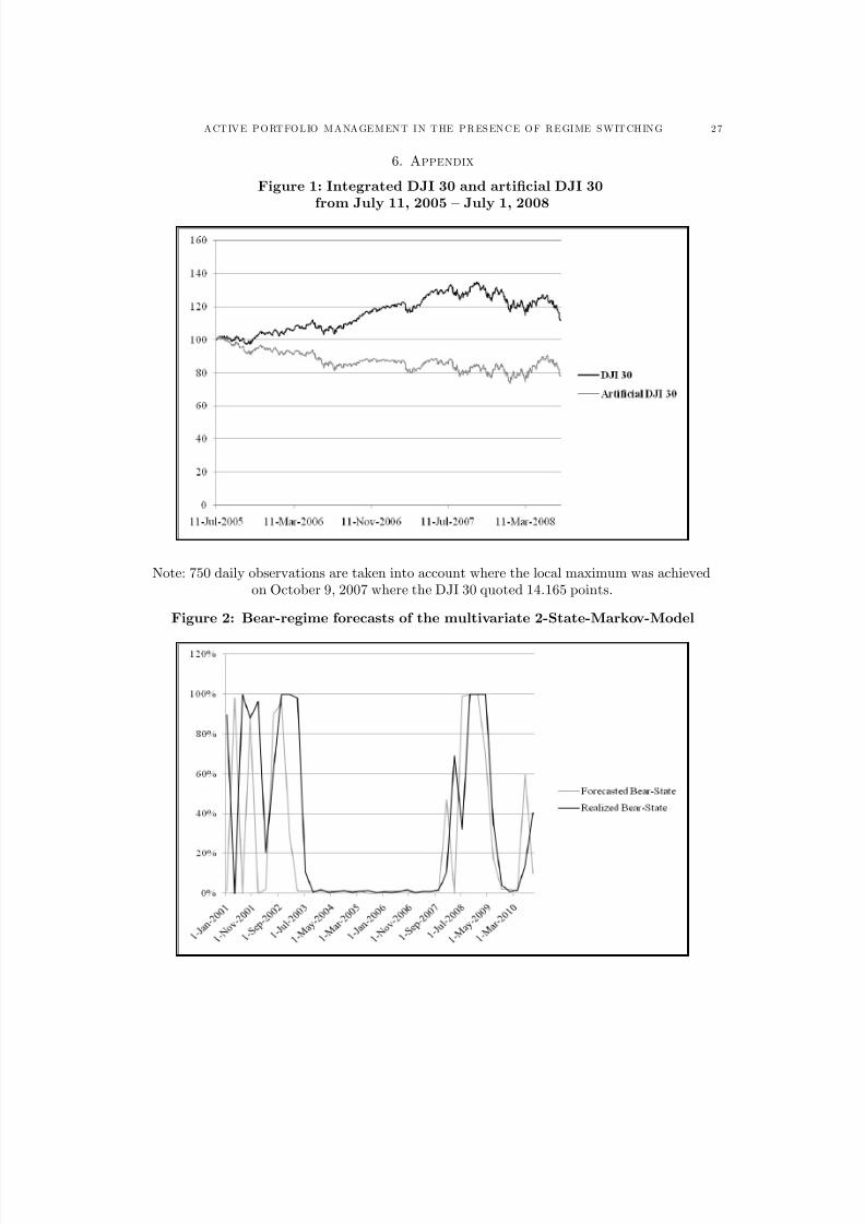
as the ones of Alexander and Dimitriu (2005a,b) and Grobys (2010) 2. Equations (6) and (7)involve that the linear trend is first subtracted from the market returns and switches thedirection at point max. Subtracting a linear trend term until max and adding the term fromthe local maximum onwards results in an artificial index that is below the corresponding stockindex until max and exhibiting higher returns as the underlying index from max onwards asthe bubble (i.e. the peak of the preceding bull market) disperses (Figure 1). Furthermore,

2However, Alexander (1999) and Alexander and Dimitriu (2005a, b) use an OLS-regression from the log-stock prices on the stock index in logs in order to replicate the S&P 500 index (Alexander and Dimitriu 2005a),whereas Grobys (2010) estimates a restricted maximum-likelihood function. Under Gaussian assumption, theestimators should be similar.



20 KLAUS GROB YS

the integrated time series of the stocks employed to track the artificial indices are in line withGrobys (2010) given by

= + X=1

(8)

where denotes the ordinary daily return of stock at time and is a constant term where ∈ ¤+ is chosen such that 0 ∀ = 1 and = 1. Then, the log- likelihoodfunction used to estimate the optimal weight allocation that is assumed to exhibit defensiveproperties within the out-of-sample period is given by

ln ( ) = −

2 log(2) −

2 log 2

− 1

2

X∈

(22

) (9)

where 2 = −

P=1 · and =

©; 2

ª. Following Alexander and Dimitriu (2005a)

and van Montfort, Visser and Fijn van Draat (2008), it is usual to impose restrictions. In thefollowing though it will be assumed to be sufficient to restrict the weights to sum up to one andto be positive (i.e. prohibition of short selling) which is given by

0 (10)

for = 1

X=1

= 1 (11)

The estimation procedure that is associated with defensive strategies may require allocatinghigh weights to stocks which exhibit defensive properties. Therefore, the only restriction which

is of importance is the positivity restriction concerning the weights. Once estimated, the weights are held constant as long as the investor faces a bear market regime which is examinedquarterly.

Once a bull market regime is ascertained equations (6) and (7) will be substituted by equation(12) because the index which is tracked rests simply upon the integrated time series given by

= +X

=1

(12)

As long as the Markov-Switching model does not suggest a change of the regime (i.e. fromthe current bull to bear market regime), the portfolio will be rebalanced semi-annually whiletaking into account equations (8)-(10). In comparison to the active asset allocation strategydescribed by equations (1)-(12), the strategy which does not account for equations (1)-(7) will

be referred to as passive asset allocation strategy and acts as a benchmark when the models’performances are compared. The passive strategy is rebalanced semi-annually only, irrespectiveif the investor faces a bull- or bear market regime. However, the passive strategy is supposedto be associated with lower transaction costs. The investor may expect higher transaction costsas the position he takes becomes more defensive, that is, the chosen factor is larger.

3. THE DATA

The analysis is based on two stock markets (i.e. N=2), the American and the Europeanone, represented by the DJI 30 and the OMX 30, respectively. The source of the data is acost free one: www.finance.yahoo.com and www.nasdaqomxnordic.com. These indices are also




considered in the multivariate 2-State-Markov-Switching model in Grobys’ (2011) study3. Inline with Guidolin and Timmermann (2008), monthly (i.e denoted by ) stock market data (i.e.in log-returns) is employed to estimate the 2-State-Markov-Switching. 171 Monthly observation

from November 3, 1986 to January 2, 2001 could be employed in order to forecast the currentregime on January, 2001. The forecast concerning the next quarter though accounts for datauntil April 2, 2001 and, hence, includes 174 monthly observations and so on. The regimeforecasts are repeated on a quarterly base4. For instance, if the model suggests in the first stepa bear market regime like on April 2, 2001 (see equations (1)-(4)), the optimization proceduretakes into account equations (6)-(7) in the second step. Since the market regime is estimatedto switch to a bull market regime on July 2, 2001, equation (12) is taken into account in theoptimization procedure (Table 1). However, if the investor had been situated in a bull marketin both times, equation (12) would have been employed on April 2, 2001 and the weights wouldhave not been updated on July 2, 2001 because the investor rebalances the portfolio weightsonly every second quarter as long as he/she faces a bull market.

4. DISCUSSION OF THE RESULTS

The models are estimated for = 2, where = 1 denotes the bull state and = 2 denotesthe bear state. According to the HQ-and SC-criterion, the lag order is = 0, which is inline with the common finding that stock market returns of developed countries do not exhibitpatterns of autocorrelation5. The statistical test for contemporaneous correlation uses 10 yearsof daily frequency data running from January 2, 1991 until December 29, 2000 corresponding to2457 observations. This time window used to estimate the correlation covers 10 years of the in-sample window in daily terms. The correlation between the DJI 30 and the OMX 30 log-returnsis estimated to be = 02910. Hence, the test statistic = 20802(p-value 0.0000)shows that the null hypothesis is clearly rejected. Due to the significant correlation between DJI30 and OMX 30, a bivariate 2-State-Markov-Switching model is used. Consequently, the currentregime is estimated simultaneously on a quarterly base (i.e. = 3 and = 40 1), beginningon January 2, 2001. The out-of-sample time window runs from January 2, 2001 to January 3,

2011 (i.e. = 120). While the covariance-matrices are assumed to be constant during eachregime, the 2-State-Markov-Switching model transforms contemporaneous correlation into time-varying covariances, as the regimes are dependent on the time . Equations (13)-(17) show theestimates of the 2-State-Markov model concerning equations (2)-(4) (standard errors are givenin parenthesis) and taking into account the overall sample (i.e. November 3, 1986 — January 3,2011):

µ 30130 1

¶=

⎛⎜⎜⎝

00062(00010)

00092(00017)

⎞⎟⎟⎠+

µ 3030

¶ (13)

for S1

3From an economical point of view it can be assessed that 3.34% of Sweden’s imported goods in 2010were produced in the USA, whereas in the corresponding period 7.29% of all produced goods in Sweden wereexported to the USA. Consequently, the USA is apart from Germany, Norway and the United Kingdom one of Sweden’s largest trade partners (see www.scb.se). In the present study it is assumed that such interactions arealso embedded in a simultaneous movement of the economies’ stock indices, which is sometimes referred to asinternational stock market integration.

4The strategy assumes that regimes are persistent. If the expected duration of each regime is longer thanthe update of the current regime estimate (i.e. every quarter), the investor assumes here that the regime is notchanging until the next update.

5The Hannan-Quinn (HQ) and Schwarz (SC) criterion are selection criteria concerning the optimal lag-orderin a VAR- model.



22 KLAUS GROB YS

µ 301

30 1¶ =

⎛

⎜⎜⎝

−00066(00034)

−00127(00051)

⎞

⎟⎟⎠+ µ 30

30¶ (14)

for 2

X 1

=

⎛⎜⎜⎝

190 − 04(200 − 05)

−100 − 05(200 − 05)

−100 − 05(200 − 05)

430 − 04(200 − 05)

⎞⎟⎟⎠ (15)

for 1

X 2

=

⎛

⎜⎜⎝850 − 04

(130 − 04)400 − 05

(150 − 04)

400 − 05(150 − 04)

179 − 03(310 − 04)

⎞

⎟⎟⎠ (16)

=

⎛⎜⎜⎝

094(005)

017(006)

006(002)

083(004)

⎞⎟⎟⎠ (17)

The expected duration of the bull market regime is estimated at 16.53 months, whereasthe corresponding figure concerning the bear market regime is estimated at 5.86 months. Thecovariance matrix in the Markov-Switching model is dependent on the current regime and,hence, time-varying. Equations (15) and (16) show that the monthly covariance is estimatedto be negative across these stock markets during bull states and positive during bear states.

Estimating the quarterly updated (i.e. a rolling time window and = 3) 2-State-Markov modelfrom January 2, 2001 onwards suggests bear-market forecasts as given in figure 2. Figure 2shows the estimated regime including the whole sample as given by equations (12) — (14) andthe forecasted bear market regime where only information until time − ( − · ) is takeninto account. A probability threshold of 0.90 implies that the defensive strategy is appliedonly if the bear-market state probability forecast in the current quarter exceeds the threshold.Table 1 shows the asset allocation suggested by this approach for the out-of-sample period.The forecast covers ten years, January 2, 2001 - January 3, 2011. To estimate the maximumlikelihood function concerning equations (4)-(10), 750 days of daily frequency data is employedwhich is in line with Alexander and Dimitriu (2005a). The active strategy indicates a defensiveweight allocation strategy for April 2, 2001, October 1, 2001, July 1, 2002 and July 1, 2008(see table 1 in association with figure 2) and five diff erent portfolios will be estimated for bothstock markets. Thereby, the factor varies between those estimated portfolio weight allocations

where ∈ {004 008 012 016 020}. Thus, portfolio 1 (i.e. for each stock market) accountsfor 1 = 004which corresponds to the enhancing factor being added, respectively, subtracted(see equations (6) and (7)) by 10% in annual terms.

Analogously, the enhancement factor 2 = 008 of portfolio 2 corresponds to an active assetallocation strategy, where the artificial index tracked deviates 20% from the ordinary indexand so on (Figure 1).Table 2 shows that defensive asset allocation strategies which suggestdeviations from the ordinary index between 40%-50% performed the best concerning strategiesrelated to the DJI 30. All actively managed portfolios (i.e. portfolio 1 — portfolio 5) outperformthe benchmark which is portfolio 0 (Figure 3). The latter is an ordinary index tracking portfoliowhere the weights are re-estimated semi-annually, irrespective of the current regime. However,this passive asset allocation strategy still dominates the stock index as the Sharpe ratio (i.e.




0.28) is twice as much as the DJI 30’s Sharpe ratio which was 0.14 within the overall out-of-sample period.

However, the results diff er concerning the Swedish stock market. The higher the deviation the

lower the Sharpe ratios when the whole out-of-sample period is considered. Here, the ordinaryindex tracking portfolio (i.e. portfolio 0) dominates all active asset allocation strategies as wellas the index as its Sharpe ratio of 0.20 is higher in comparison to actively managed portfolios 6.

In order to determine if the latter outcome can be traced back to the active strategy itself or if this outcome is rather a fact of dataset limitations concerning the dataset of stocks, a sub-sampleperiod will be investigated. The 2-State-Markov model suggests the latest bear market fromJuly 1, 2008 — April 1, 2009 as shown in figure 2 and table 1. As the equity prices began to fallalready before July 1, 2008, a sample including data from October 1, 2007-March 31, 2009 willbe considered. Consequently, this time window also covers the financial crisis period in 2008.Table 3 shows that the DJI 30 had a return of -9.33% p.a. within this period, whereas the OMX30 exhibited a return of -8.33%. Considering the US-stock market, portfolios 4 and 5 dominatethe benchmark portfolio as the increase in return being 75.68% corresponds to a marginalincrease of 5.26% in volatility only (the corresponding figures concerning portfolio 5 are 76.62%

increase in returns associated with 7.43% increase in volatility). Considering the Swedish stockmarket, the benchmark portfolio exhibits a return of -7.32% p.a. with an annual volatility of 15.43%. However, portfolio 2 exhibits 24.70% higher annual returns, associated with an increaseof 16.01% in volatility and thus dominates the benchmark portfolio7. Consequently, the reasonfor diff erences concerning the strategies performances given diff erent stock indices can be tracedback to dataset limitations since it was not possible to replicate stochastic processes such asgiven by the defensive artificial indices being tracked. In particular, the period April 2, 2001 —April 1, 2003 shows an underperformance of these defensive asset allocation strategies (see figure2). The underperformance of the defensive strategies concerning the Swedish stock market canbe attributed to both the bias regarding the preselected stocks (i.e. only 17 of 30 stock could beaccounted for) and the reliability of the forecasted regime since the regime-switching model’sforecasted regimes exhibited lower deviations from the realized regimes during the second partof the out-of-sample window (i.e. 31% deviation on average during Jan 2001-Dec 2005 and 14%

deviation during Jan 2006-Dec 2010). Furthermore, tables 2 and 3 show that the trading costsincrease as a function of the trading volume. The more defensive the taken positions in stocks,the higher the trading volume and, as a consequence, the higher the trading costs.

Although the common academic literature predominately takes large capitalization stockindices into account in the context of empirical stock market analyses, it could be shown herethat also smaller European stock indices such as the Swedish stock index OMX 30 switchescontemporaneously with the US-stock market from bull to bear markets and vice versa. Thus,the studies of Ang and Baekert (2002a) can be supported. However, the bivariate model mayaccount for any combination of stock markets that are highly correlated such as the German’sleading index DAX 30, and the DJI 30 or the British’s leading index FTSE 100 and the DJI 30or DAX 30. The bivariate DJI 30 — OMX 30 model is selected for illustration purposes and inorder to stand out from common studies. Apart from accounting for time-varying correlationsbetween international stock markets, under the bivariate setup the states are more persistentfor the US stock market (Table 4). However, the bivariate model does not determine whichindex drives the variable that initiates switches of the states even though it may be assumedthat the US-stock index involves the hidden factor. This may be subject to future research.

The operational criterion suggests at four points of time a bear market which implies adefensive asset allocation (Table 1). The bear market regime in the wake of the financial crisis

6Note that the 29 out of 30 stocks are accounted for when running the maximum likelihood function con-cerning the DJI 30 index. Due to data set limitations though 17 out of 30 stocks could be taken into accountonly when running the optimization procedure with respect to the OMX 30 as the access to stock data becomesthe more limited the further away the historical selected data.

7These results hold even if the net returns (i.e. after transaction costs) are taken into account.



24 KLAUS GROB YS

is estimated by far be more persistent as the stock market crash of 2001-2002. In contrastto Alexander and Dimitriu (2005a, b), the ordinary cointegration portfolio is employed asbenchmark in order to analyze the performance diff erences.

In contrast to Guidolion and Timmermann (2008) in this study only two states (i.e. bulland bear market) are taken into account which is also in line with Ang and Baekert (2002a),as active portfolio management typically diff erentiates only between off ensive and defensivestrategies where defensive strategies are employed when market participants face bear markets.The present study suggests an ordinary index tracking strategy based on cointegration if themanagement faces a bull market, whereas defensive strategies are employed in case of a bearmarket. However, off ensive strategies may also involve enhanced index tracking strategies assuggested by Alexander and Dimitriu (2005a) or Grobys (2010). This could even improvethe overall index tracking portfolio’s performance. Alexander and Dimitriu (2005a) point outthat tracking the artificial indices by more than plus/minus 5% does not result in an equityportfolio with higher Sharpe ratios as the portfolio’s volatility increases and the abnormalreturns become insignificant. This outcome cannot be supported in this study which takes intoaccount the market regime: Considering the US-stock market, table 2 shows that the Sharpe

ratios increase as increases (see also figure 4). The latter can be seen as market anomalieswhich may appear due to overreactions during bear market regimes.

Furthermore, this study employs monthly stock market data for estimating the current mar-ket regime (i.e. step one in the procedure). Such data frequency is also used in the 4-StateMarkov-Switching framework suggested by Guidolion and Timmermann (2008). However, thedata set contains, due to data set limitations, fewer observations (i.e. 292 monthly observa-tions) in comparison to the study of Guidolion and Timmermann (2008), who account for 552monthly observations. As 14 parameters are estimated only, the data set limitations do notdelimitate the parameter estimation results. The estimated parameters are clearly significantas provided by equations (13)-(17).

The second step of the optimization procedure, which estimates the optimal weight allocationof the artificial index, uses linearized stock prices. It is worth observing that no excess returnsare gained if either ordinary returns, log-returns or log-prices are employed in the maximum-

likelihood function. This shows that linearized prices, as suggested by Grobys (2010), are auseful tool in order to cache assets’ short term momentum (see De Bondt and Thaler, 1985,Chopra et al., 1992 and Jegadeesh and Titman, 1993).

Ang and Baekert’s (2002a) findings that United States and the United Kingdom face thesame regime shifts generated by the benchmark regime-switching model can be supported inthe sense that the Swedish stock market and the US-stock market are driven by the samestochastic variable into bull and bear market regimes. Another outcome of Ang and Baekert(2002a), namely that in one regime the equity returns exhibit a lower conditional mean, muchhigher volatility, and are more highly correlated compared to the other regime, can be supportedas well (see equations (13)-(17)). In contrast to Ang and Bekaert (2002a) though, in this studythe regime switching variable is treated as unobservable which is in line with Guidolin andTimmermann (2008), Alexander and Dimitriu (2005b) and Grobys (2011).

5. CONCLUSION

Accounting for actively managed defensive strategies enhances the gains of the equity port-folio. Even though passive strategies suggest an implicit market timing factor due to an equi-librium eff ect (Alexander and Dimitriu, 2005b), the present study shows that when taking intoaccount diff erent regimes active strategies perform better. The model for the US stock mar-ket clearly shows that in bear markets the actively managed equity portfolios outperform thecommon cointegration based portfolio by successfully capturing the stochastic short-run trends.The maximum-likelihood function that is constructed to extract stock prices following contrarytrends to the index, pitches on stocks that exhibit defensive movements. For instance on July1, 2008 portfolio 5 (i.e. concerning the US-market) suggests an asset allocation of 100% to the




stock “The home Depot, Inc.” which belongs to the furniture selling industry. The higher thedeviation of the artificial index selected, the more weight is allocated to this stock8. Similarpatterns can be investigated on the Swedish stock market and the stock company “Securitas”

which provides security services. However, there remains demand for future research to deter-mine the linkages between the asset allocation which is estimated by this maximum-likelihoodprocedure and the stock price dispersion. Furthermore, the Markov-Switching model couldaccount for three states, for instance, where the bull- and bear market state is extended by astate capturing a potential sideward movement of the index. The actively managed portfoliomay diff erentiate between strategies such as enhanced index tracking if the Markov-Switchingmodel predicts a bull market, defensive index tracking strategies if the investor faces a bearmarket and an ordinary index tracking strategy otherwise.

References

[1] Ang A., & Bekaert, G. (2002a). International Asset Allocation With Regime Shifts. Review of FinancialStudies (15)/4, pp. 1137-1187.

[2] Ang, A. & Bekaert, G. (2002b). Regime Switches In Interest Rates. Journal of Business and Economic

Statistics (20), pp. 163-182.[3] Ang A., & Chen, J. (2002). Asymmetric Correlations Of Equity Portfolios. Journal of Financial Economics(63), pp. 443-494.

[4] Alexander C. (1999). Optimal Hedging Using Cointegration. Philosophical Transactions of the Royal SocietySeries A, 357, pp. 2039-2058.

[5] Alexander, C. & Dimitriu, A. (2005a). Indexing And Statistical Arbitrage. The Journal of Portfolio Man-agement (31)/2, 50-63.

[6] Alexander, C. & Dimitriu, A. (2005b). Indexing, Cointegration And Equity Market Regimes. InternationalJournal of Finance and Economics (10), pp.213-231.

[7] Barberis, N. (2000). Investing For The Long Run When Returns Are Predictable, Journal of Finance (55),pp. 225-264.

[8] Black, F. (1972). Capital Market Equilibrium With Restricted Borrowing. Journal of Business (45), pp.444-454.

[9] Black, F., & Litterman, R. (1992). Global Portfolio Optimization, Financial Analysts Journal (48), pp.28-43.

[10] Boldin, M., & Cici, G. (2010). The Index Rationality Paradox. Journal of Banking and Finance (34), pp.

33-43.[11] Claessens, S., Kose, M.A., & Terrones, M.E. (2009). What Happens During Recessions, Crunches And

Busts? Economic Policy (60), pp.653-700.[12] Chow, G. (1995). Portfolio Selection Based On Return, Risk, And Relative Performance Financial Analysts

Journal (51)/ 2, pp. 54-60.[13] Chopra, N., Lakonishok, J., & Ritter, J., (1992). Measuring Abnormal Performance. Do Stocks Overreact?

Journal of Financial Economics (31), pp. 235–268.[14] De Bondt, W., & Thaler, R., (1985). Does The Stock Market Overreact? Journal of Finance (40), pp.

793–805.[15] Friesen, G.C., Weller, P.A., & Dunham, L.M. (2009). Price Trends And Patterns In Technical Analysis: A

Theoretical And Empirical Examination. Journal of Banking & Finance (33), pp. 1089-1100.[16] Gonzalez, L., Powell, J. G., Shi, J., & A. Wilson (2005). Two Centuries of Bull And Bear Market Cycles.

International Review of Economics and Finance (14), pp. 469–486.[17] Granger, C.W.J., & Terasvirta, T. (1993). Modelling Nonlinear Economic Relationships, Chapter 5. Oxford:

Oxford University Press.

[18] Grobys, K. (2010). Do Business Cycles Exhibit Beneficial Information For Portfolio Management? AnEmpirical Application Of Statistical Arbitrage. The Review of Finance and Banking (2)/2, pp. 41-56.

[19] Grobys, K. (2011). Are Diff erent National Stock Markets Driven By The Same Stochastic Hidden Variable?The Review of Finance and Banking (3)/1, pp. 21-30.

[20] Guidolin, M., & Timmermann, A. (2005a). Strategic Asset Allocation And Consumption Decisions UnderMultivariate Regime Switching, Federal Reserve B ank of St. Louis working paper No. 2005-002A.

[21] Guidolin, M., & Timmermann, A. (2005b). Size And Value Anomalies Under Regime Switching. FederalReserve Bank of St. Louis working paper No. 2005-007A.

8The weight allocation vector July 1, 2008 concerning the stock „The Home Depot, Inc.“ for the portfolios(0, 1,. . . ,5) is given by (6.85%, 17.92%, 59.56%, 82.61%, 94.83%, 100%). At this time, the Markov-Switchingmodel predicts a bear market with probability 90% and consequently, the weights are held constant as longas the regime is not switching (i.e. 3 quarters in this case).



26 KLAUS GROB YS

[22] Guidolin, M., & Timmermann, A. (2006a). An Econometric Model Of Nonlinear Dynamics In The JointDistribution Of Stock And Bond Returns. Journal of Applied Econometrics (21), pp.1-22.

[23] Guidolin, M., & Timmermann, A. (2006b). Term Structure Of Risk Under Alternative Econometric Speci-fications. Journal of Econometrics (131), pp. 285-308.

[24] Guidolin, M., & T immermann, A. (2006c). International Asset Allocation Under Regime Switching, SkewAnd Kurtosis Preferences. Federal Reserve Bank of St. Louis working paper No. 2005-018A.

[25] Guidolin, M., & Timmermann, A. (2008). Asset Allocation Under Multivariate Regime Switching. Journalof Economic Dynamics and Control (31), pp. 3503-3544.

[26] Hamilton, J. (1989). A New Approach To The Economic Analysis Of Nonstationary Time Series And TheBusiness Cycle. Econometrica (57), pp. 357-384.

[27] Jegadeesh, N., & Titman, S., (1993). Returns To Buying Winners And Selling Losers: Implications ForStock Market Efficiency. Journal of Finance (48), pp. 65–91.

[28] Jones, R.C., Lim, T., & Zangari, P.J. (2007). The Black-Litterman Model For Structured Equity Portfolios.The Journal of Portfolio Management (33)/2, pp. 24-33.

[29] Lunde, A., & Timmermann, A. G., (2004). Duration Dependence In Stock Prices: An Analysis Of BullAnd Bear Markets. Journal of Business & Economic Statistics (22)/3, pp.253–273.

[30] Markowitz, H. (1959). Portfolio Selection: Efficient Diversification of Investments. New York: John Wiley& Sons.

[31] Martellini, L., & Ziemann, V. (2007). Extending Black-Litterman Analysis Beyond The Mean-Variance

Framework. The Journal of Portfolio Management (33)/4, pp. 33-44.[32] Montfort, K., Visser, E., & Fijn van Draat, L. (2008). Index Tracking By Means Of Optimized Sampling.

Journal of Portfolio Management (34), pp.143-151.[33] Sharpe, W. (1964). Capital Asset Prices: A Theory Of Market Equilibrium Under Conditions Of Risk.

Journal of Finance, pp, 425-442.[34] Pagan, A. R., & Sossounov, K. A. (2003). A Simple Framework For Analyzing Bull And Bear Markets.

Journal of Applied Econometrics (18)/1, pp. 23–46.[35] Perez-Quiros, G. & Timmermann, A. (2001). Business Cycle Asymmetries In Stock Returns: Evidence

From Higher Order Moments And Conditional Densities, Journal of Econometrics (103), pp. 259-306.[36] Phengpis, C., & Swanson, P.E. (2011). Optimization, Cointegration And Diversification Gains From Inter-

national Portfolios: An Out-Of-Sample Analysis. Review of Quantitative Finance and Accounting (36)/2,pp.269-286.

[37] Van Montfort, K., Visser, E., & Fijn van Draat, L. (2008). Index Tracking By Means Of Optimized Sampling.The Journal of Portfolio Management (34)/2, pp. 143-152.

[38] Whitelaw, R. (2001). Stock Market Risk And Return: An Equilibrium Approach. Review of Financial

Studies (13), pp. 521-548.




6. Appendix

Figure 1: Integrated DJI 30 and artificial DJI 30from July 11, 2005 — July 1, 2008

Note: 750 daily observations are taken into account where the local maximum was achievedon October 9, 2007 where the DJI 30 quoted 14.165 points.

Figure 2: Bear-regime forecasts of the multivariate 2-State-Markov-Model



28 KLAUS GROB YS

Figure 3: Defensive portfolios and the OMX 30 in the out-of-sample period

Figure 4: Defensive portfolios and the DJI 30 in the out-of-sample period




Table 1: Active weight allocation strategies suggested by the Markov-Switchingmodel

Date Action Date Action

2-Jan-2001 1 3-Jan-2006 32-Apr-2001 2 3-Apr-2006 12-Jul-2001 1 3-Jul-2006 31-Oct-2001 2 2-Oct-2006 12-Jan-2002 1 3-Jan-2007 31-Apr-2002 3 2-Apr-2007 11-Jul-2002 2 2-Jul-2007 31-Oct-2002 4 1-Oct-2007 12-Jan-2003 4 2-Jan-2008 31-Apr-2003 1 1-Apr-2008 11-Jul-2003 3 1-Jul-2008 21-Oct-2003 1 1-Oct-2008 42-Jan-2004 3 2-Jan-2009 4

1-Apr-2004 1 1-Apr-2009 11-Jul-2004 3 1-Jul-2009 31-Oct-2004 1 1-Oct-2009 13-Jan-2005 3 4-Jan-2010 31-Apr-2005 1 1-Apr-2010 11-Jul-2005 3 1-Jul-2010 33-Oct-2005 1 1-Oct-2010 1

Asset allocation strategies:1. The weight allocation being selected is an ordinary index-tracking strategy.2. The weight allocation being selected is in accordance to a defensive strategy.3. The weight allocation being selected is the ordinary index-tracking strategy which is

estimated in the previous period (i.e. the weights are held constant).

4. The weight allocation being selected is the defensive weight allocation strategy whichis estimated in the previous period (i.e. the weights are held constant).

Table 2: Statistical properties and performances in the out-of-sample periodBenchmark DJI 30Asset DJI 30 Portfolio

0Portfolio1

Portfolio2

Portfolio3

Portfolio4

Portfolio5

Gross re-turn p.a.

2,38% 6,20% 6,65% 8,67% 8,97% 9,51% 9,45%

Volatilityp.a.

17,11% 19,61% 18,58% 16,68% 16,15% 16,48% 16,37%

Sharpe ra-

tio (beforecosts)

0,14 0,32 0,36 0,52 0,56 0,58 0,58

Transactionvolume p.a.

- 87% 120% 171% 190% 197% 199%

Tradingcosts p.a.

- 0,70% 0,96% 1,36% 1,52% 1,58% 1,59%

Net returnp.a.

2,38% 5,50% 5,69% 7,30% 7,45% 7,93% 7,86%

Sharpe ra-tio (aftercosts)

0,14 0,28 0,31 0,44 0,46 0,48 0,48



30 KLAUS GROB YS

Benchmark OMX 30Asset OMX

30Portfolio0

Portfolio1

Portfolio2

Portfolio3

Portfolio4

Portfolio5

Gross re-turn p.a.

4,63% 6,72% 5,88% 6,12% 5,36% 3,88% 2,64%

Volatilityp.a.

24,31% 30,10% 28,94% 29,87% 29,77% 28,80% 27,75%

Sharpe ra-tio (beforecosts)

0,19 0,22 0,20 0,20 0,18 0,13 0,10


- 79% 106% 140% 171% 188% 202%

Tradingcosts p.a.

- 0,63% 0,85% 1,12% 1,36% 1,51% 1,61%

Net returnp.a.

4,63% 6,09% 5,03% 5,00% 4,00% 2,37% 1,03%


0,19 0,20 0,17 0,17 0,13 0,08 0,04

*Assuming 0.60% per 100% trading volume.

Table 3: Statistical properties and performancesduring the financial crises period

Benchmark DJI 30Asset DJI 30 Portfolio

0Portfolio1

Portfolio2

Portfolio3

Portfolio4

Portfolio5

Gross re-turn p.a.

-9,33% -9,54% -8,22% -3,81% -2,80% -2,32% -2,23%

Volatilityp.a.

10,58% 14,27% 12,08% 11,31% 13,67% 15,02% 15,33%


-0,88 -0,69 -0,68 -0,34 -0,20 -0,17 -0,15


- 87% 124% 163% 167% 176% 178%

Tradingcosts p.a.

- 0,52% 0,74% 0,98% 1,00% 1,06% 1,07%

Net returnp.a.

-9,33% -10,06% -8,96% -4,78% -3,80% -3,38% -3,30%

Sharpe ra-

tio (aftercosts)

-0,88 -0,70 -0,74 -0,42 -0,28 -0,23 -0,22




Benchmark OMX 30Asset OMX

30Portfolio0

Portfolio1

Portfolio2

Portfolio3

Portfolio4

Portfolio5

Gross re-turn p.a.

-8,12% -7,32% -5,66% -5,34% -5,64% -6,38% -5,98%

Volatilityp.a.

11,23% 15,43% 17,11% 17,90% 18,90% 21,53% 21,78%


-0,72 -0,47 -0,33 -0,30 -0,30 -0,30 -0,27


- 119% 117% 139% 155% 180% 197%

Tradingcosts p.a.

- 0,71% 0,70% 0,83% 0,93% 1,08% 1,18%

Net returnp.a.

-8,12% -8,03% -6,36% -6,17% -6,57% -7,46% -7,16%


-0,88 -0,52 -0,37 -0,34 -0,35 -0,35 -0,33

*Assuming 0.60% per 100% trading volume.Note: The period being considered here is October 1, 2007-March 31, 2009.

Table 4: Univariate MS-models estimates for the DJI 30 and OMX 30concerning the sample from November 3, 1986 — January 3, 2011*

StockIndex

State-matrix Expected durationof Bull-market

Expected durationof Bear-market

DJI 30 =

⎛⎝

095(006)

030(012)

005(002)

070(009)

⎞⎠ 18.63 months 3.38 months

OMX 30 =

⎛⎝ 095

(006)008(004)

005(003)

092(005)

⎞⎠ 19.53 months 13.22 months

* standard-error in parenthesis.

Acknowledgement. I am grateful to Professor Dr. H. Herwartz, Institute of Econometrics

and Statistics, University of Kiel for giving me useful advice and a lot of help. Furthermore, I

am grateful of having received some useful advice from an anonymous referee.

Date post:	03-Jun-2018
Category:	Documents
Upload:	ashok-chowdary-g
View:	217 times
Download:	0 times

articol2 portfolio

Documents