ARTIFICIAL INTELLIGENCE Lecturer: Silja Renooij Informed search Utrecht University The Netherlands These slides are part of the INFOB2KI Course Notes available from www.cs.uu.nl/docs/vakken/b2ki/schema.html INFOB2KI 2017-2018
Transcript
ARTIFICIAL INTELLIGENCE
Lecturer: Silja Renooij
Informed search
Utrecht University The Netherlands
These slides are part of the INFOB2KI Course Notes available fromwww.cs.uu.nl/docs/vakken/b2ki/schema.html
INFOB2KI 2017-2018
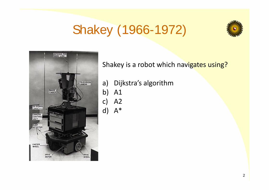
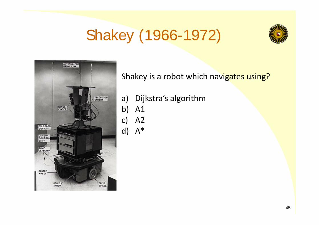
Shakey (1966-1972)
Shakey is a robot which navigates using?
a) Dijkstra’s algorithmb) A1c) A2d) A*
2
Recap: Search Search problem: States (configurations of the world) Actions and costs Successor function Start state and goal test
Search tree: Nodes represent how to reach states Cost of reaching state = sum of action costs
Search algorithm: Systematically builds a search tree Chooses an ordering of the fringe Optimal: find least‐cost plans
3
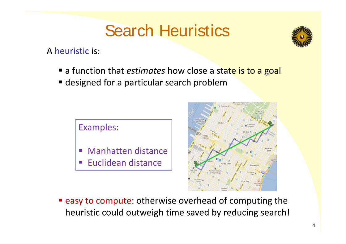
Search HeuristicsA heuristic is:
a function that estimates how close a state is to a goal designed for a particular search problem
easy to compute: otherwise overhead of computing the heuristic could outweigh time saved by reducing search!
Examples:
Manhatten distance Euclidean distance
4
Heuristic search (outline)
Best‐first search– Greedy search– A* search
Heuristic functions
Local search algorithms– Hill‐climbing search– Simulated annealing search– Local beam search– Genetic algorithms
5
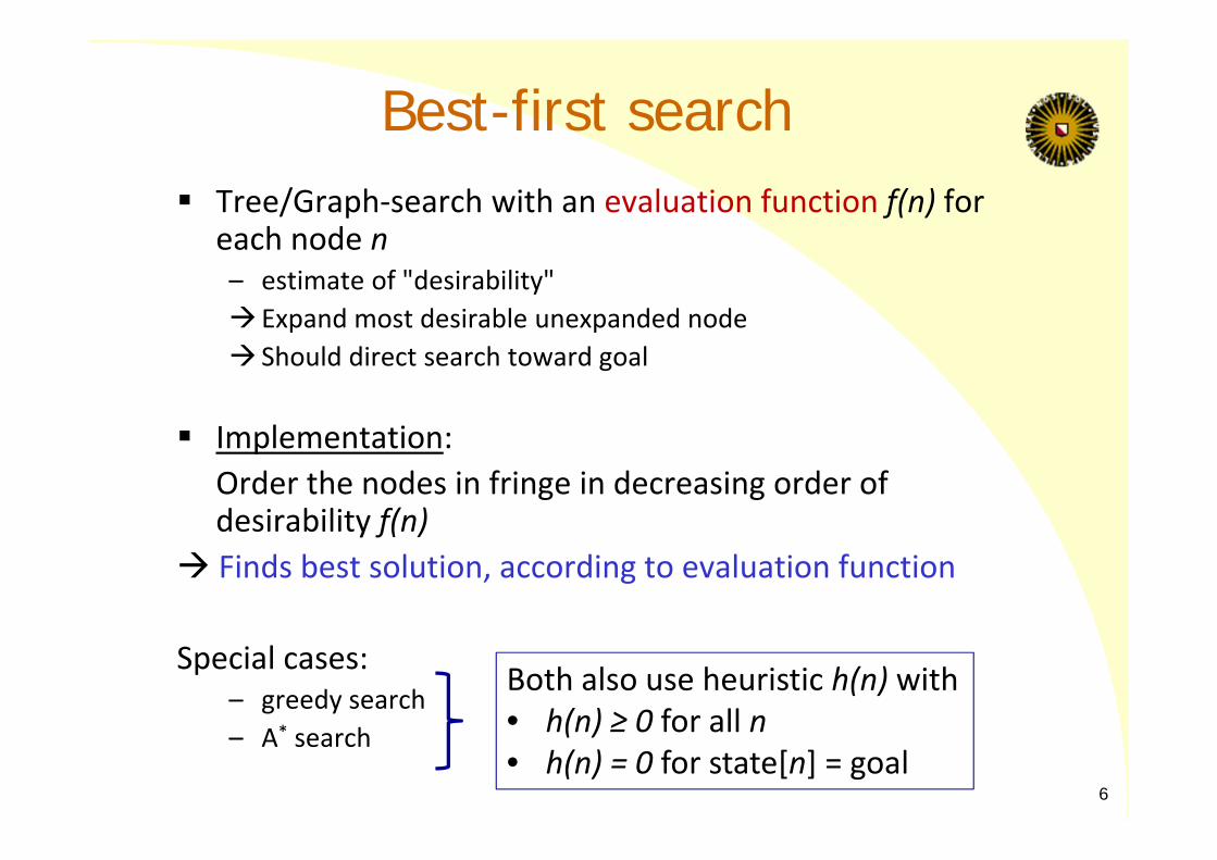
Best-first search Tree/Graph‐search with an evaluation function f(n) for
each node n– estimate of "desirability" Expand most desirable unexpanded node Should direct search toward goal
Implementation:Order the nodes in fringe in decreasing order of desirability f(n)
Finds best solution, according to evaluation function
Special cases:– greedy search– A* search
6
Both also use heuristic h(n) with• h(n) ≥ 0 for all n• h(n) = 0 for state[n] = goal
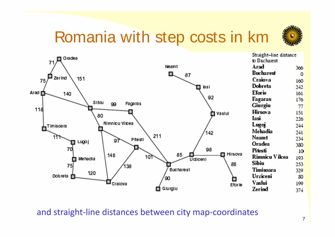
Romania with step costs in km
and straight‐line distances between city map‐coordinates7
Greedy search
Evaluation function f(n) = h(n) where – heuristic h(n) = estimated cost from n to goal
e.g., hSLD(n) = straight‐line distance from n to BucharestNote: hSLD(n) ≥ 0 for all n; hSLD(Bucharest) = 0
Greedy best‐first search expands the node that appears to be closest to goal Goal‐test: upon generation = upon expansion
8
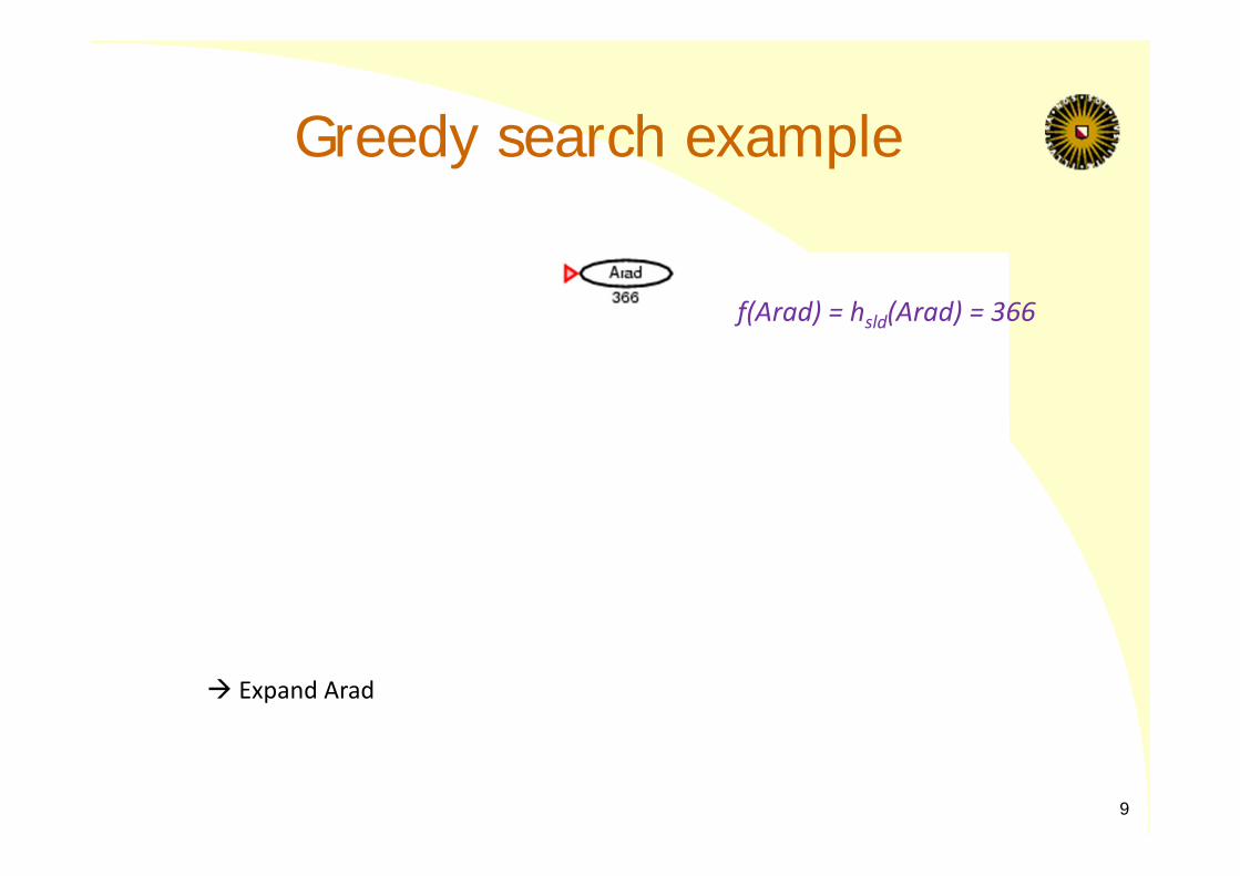
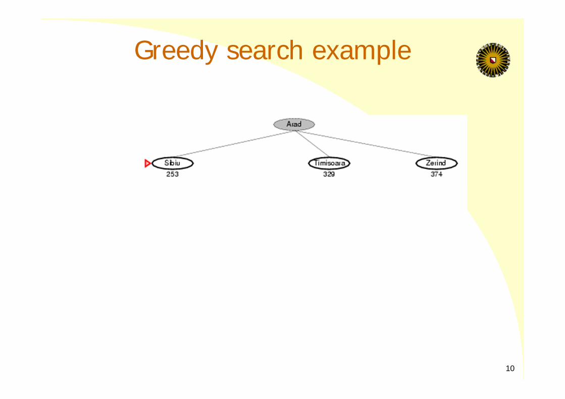
Greedy search example
f(Arad) = hsld(Arad) = 366
Expand Arad
9
Greedy search example
10
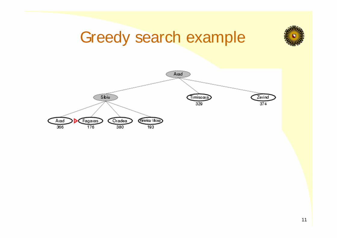
Greedy search example
11
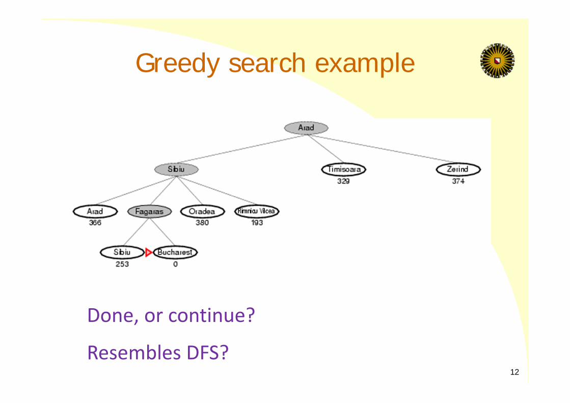
Greedy search example
Done, or continue?
Resembles DFS?12
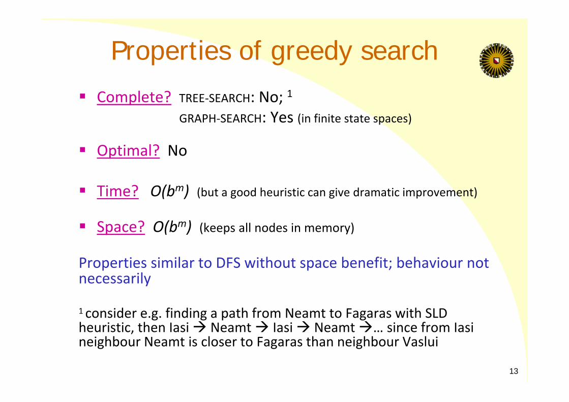
Properties of greedy search
Complete? TREE‐SEARCH: No; 1GRAPH‐SEARCH: Yes (in finite state spaces)
Optimal? No
Time? O(bm) (but a good heuristic can give dramatic improvement)
Space? O(bm) (keeps all nodes in memory)
Properties similar to DFS without space benefit; behaviour not necessarily
1 consider e.g. finding a path from Neamt to Fagaras with SLD heuristic, then Iasi Neamt Iasi Neamt… since from Iasi neighbour Neamt is closer to Fagaras than neighbour Vaslui
13
A* search
Combines benefits of greedy best‐first search and uniform‐cost search
Evaluation function f(n) = g(n) + h(n)where– g(n) = cost so far to reach n (= path cost; dynamic)– h(n) = estimated cost from n to goal (= static heuristic) f(n) = estimated total cost of path through n to goal
A* search avoids expanding paths that are already expensive
Goal‐test upon expansion!14
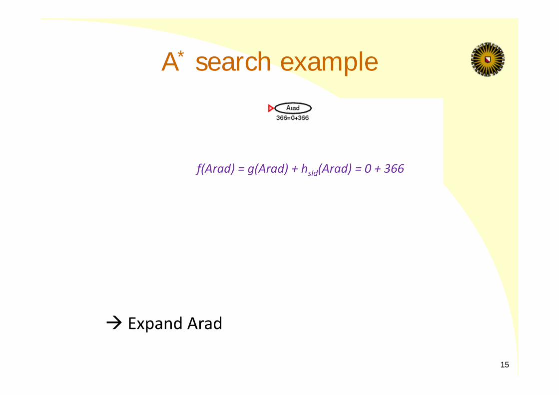
A* search example
f(Arad) = g(Arad) + hsld(Arad) = 0 + 366
Expand Arad
15
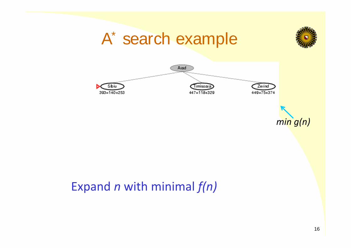
A* search example
Expand n with minimal f(n)
16
min g(n)
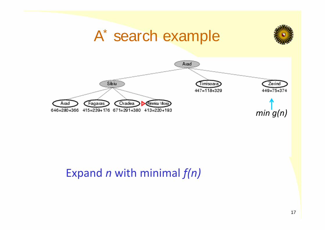
A* search example
17
min g(n)
Expand n with minimal f(n)
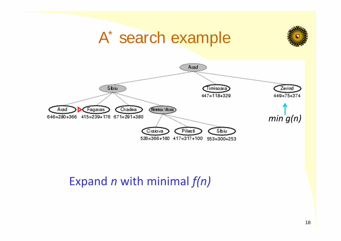
A* search example
18
Expand n with minimal f(n)
min g(n)
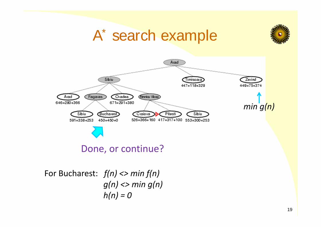
A* search example
Done, or continue?
19
For Bucharest: f(n) <> min f(n)g(n) <> min g(n)h(n) = 0
min g(n)
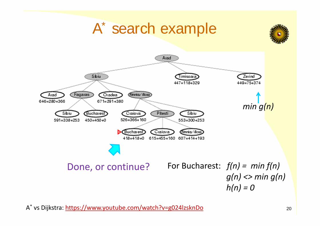
A* search example
Done, or continue?
20
min g(n)
For Bucharest: f(n) = min f(n)g(n) <> min g(n)h(n) = 0
A* vs Dijkstra: https://www.youtube.com/watch?v=g024lzsknDo
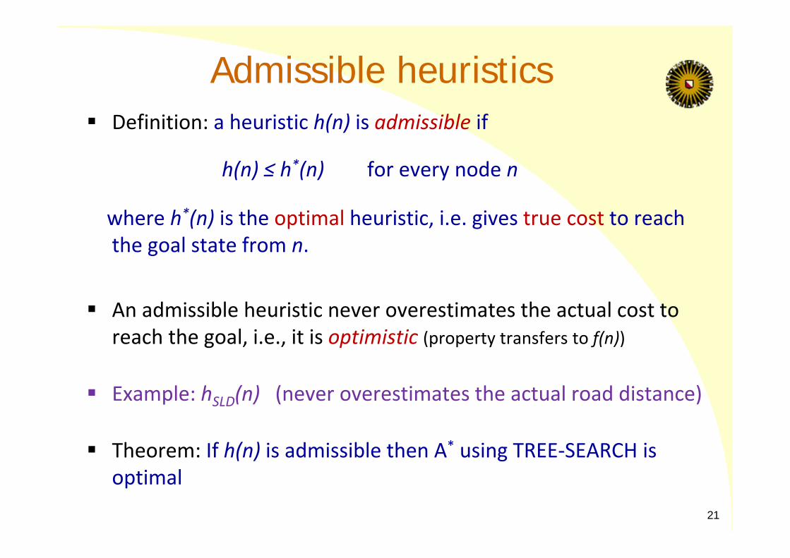
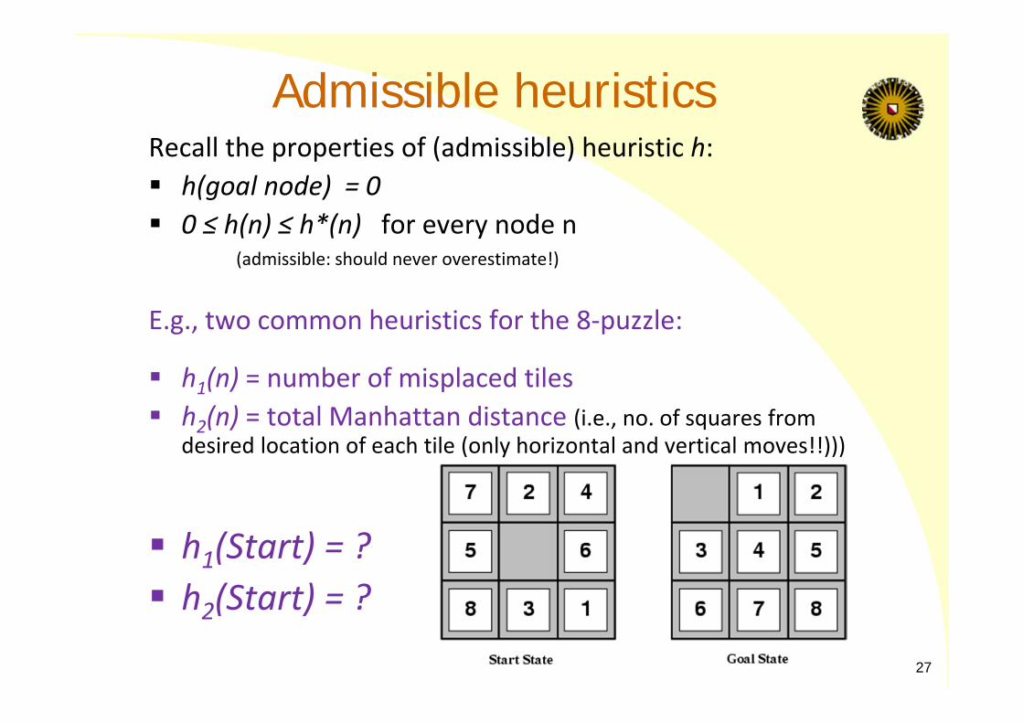
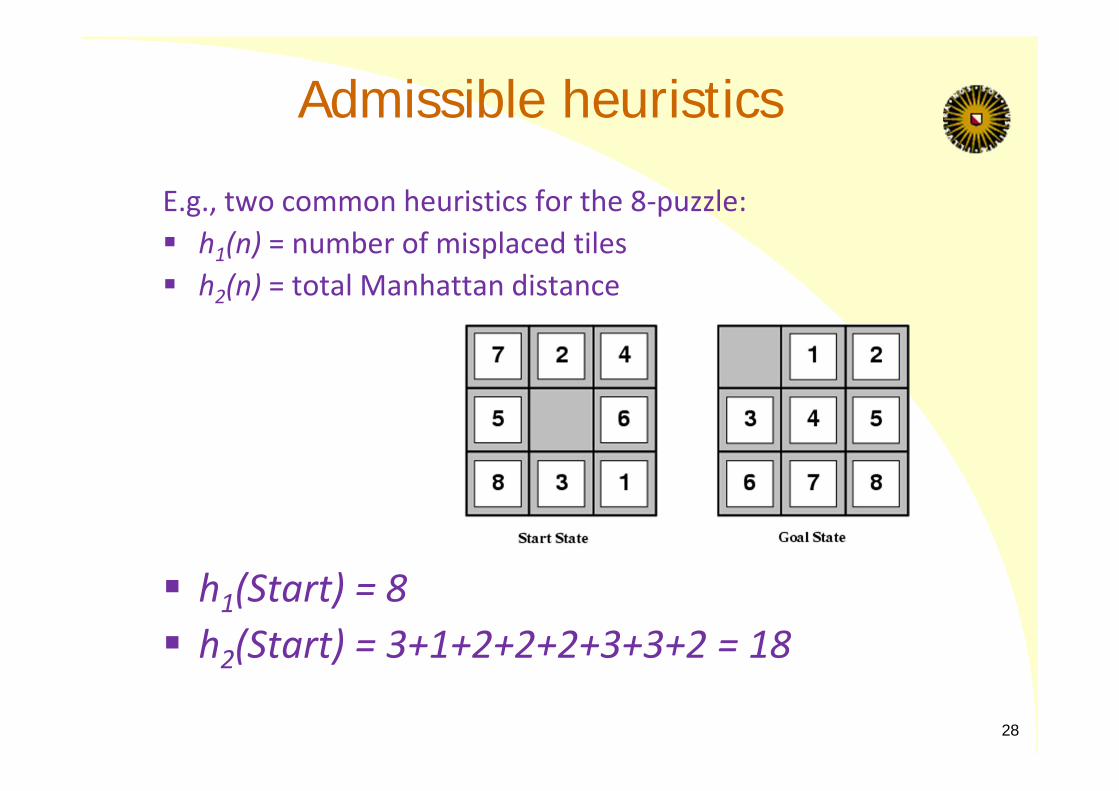
Admissible heuristics Definition: a heuristic h(n) is admissible if
h(n) ≤ h*(n) for every node n
where h*(n) is the optimal heuristic, i.e. gives true cost to reach the goal state from n.
An admissible heuristic never overestimates the actual cost to reach the goal, i.e., it is optimistic (property transfers to f(n))
Example: hSLD(n) (never overestimates the actual road distance)
Theorem: If h(n) is admissible then A* using TREE‐SEARCH is optimal
21
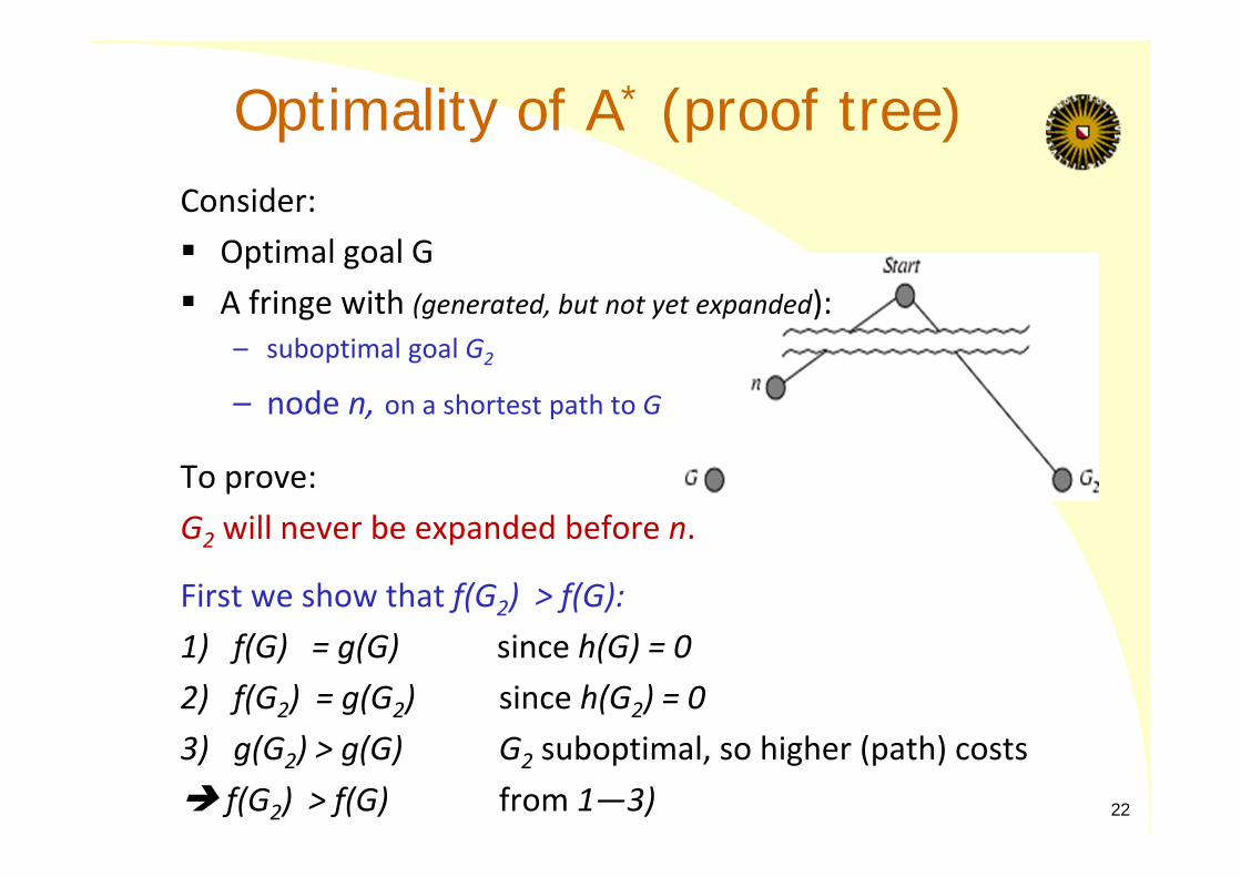
Optimality of A* (proof tree)Consider: Optimal goal G A fringe with (generated, but not yet expanded):
– suboptimal goal G2
– node n, on a shortest path to G
To prove: G2 will never be expanded before n.
First we show that f(G2) > f(G):1) f(G) = g(G) since h(G) = 0 2) f(G2) = g(G2) since h(G2) = 0 3) g(G2) > g(G) G2 suboptimal, so higher (path) costs f(G2) > f(G) from 1—3) 22
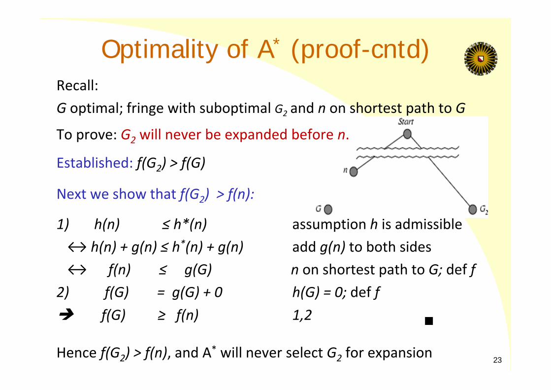
Optimality of A* (proof-cntd)Recall:G optimal; fringe with suboptimal G2 and n on shortest path to G
To prove: G2 will never be expanded before n.
Established: f(G2) > f(G)
Next we show that f(G2) > f(n):
1) h(n) ≤ h*(n) assumption h is admissible↔ h(n) + g(n) ≤ h*(n) + g(n) add g(n) to both sides↔ f(n) ≤ g(G) n on shortest path to G; def f
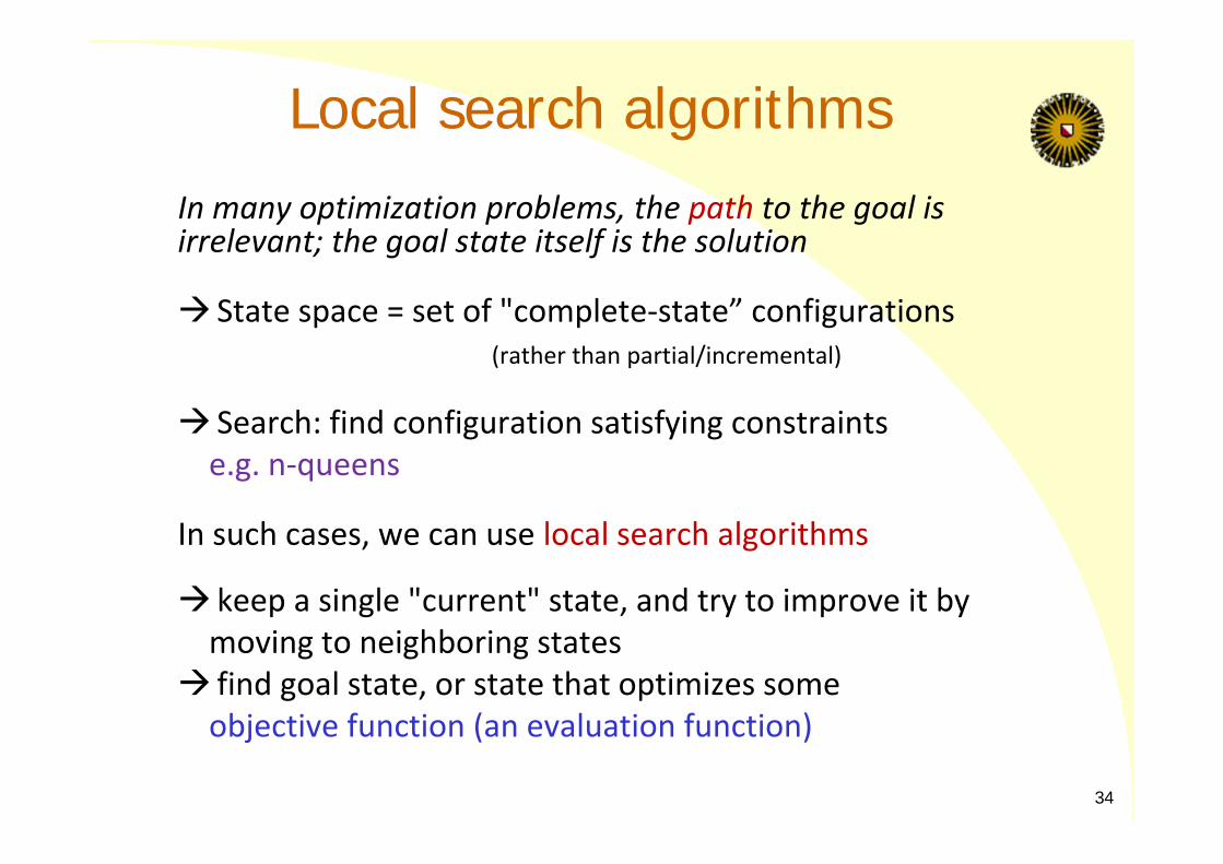
keep a single "current" state, and try to improve it by moving to neighboring states
find goal state, or state that optimizes someobjective function (an evaluation function)
34
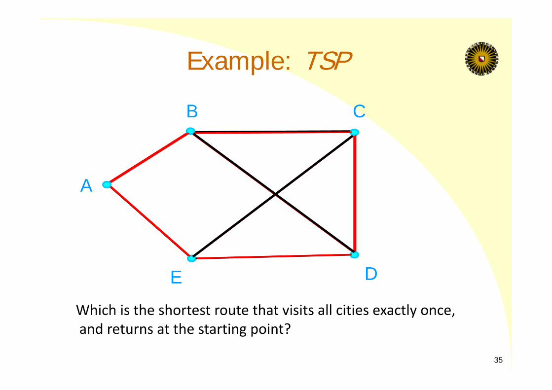
Example: TSP
Which is the shortest route that visits all cities exactly once,and returns at the starting point?
A
B C
DE
35
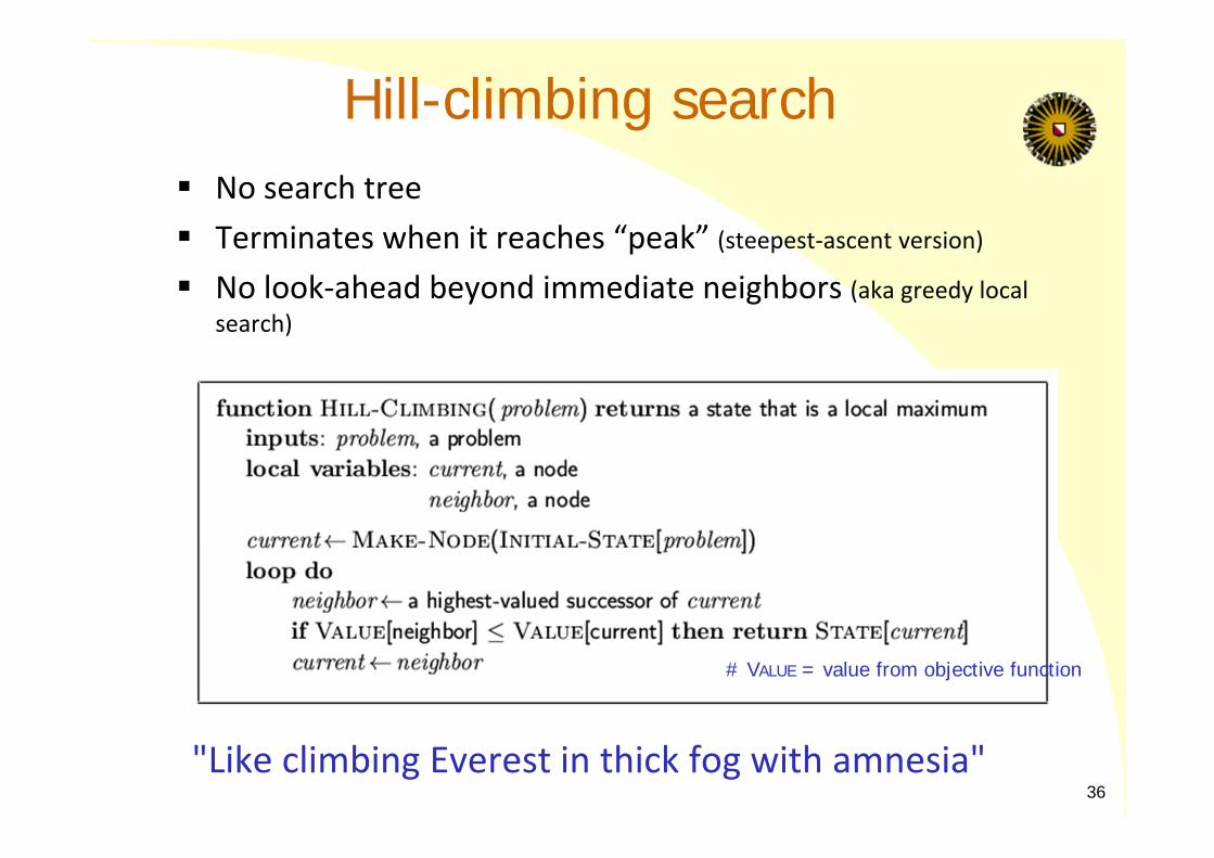
Hill-climbing search No search tree Terminates when it reaches “peak” (steepest‐ascent version) No look‐ahead beyond immediate neighbors (aka greedy local
search)
"Like climbing Everest in thick fog with amnesia"
# VALUE = value from objective function
36
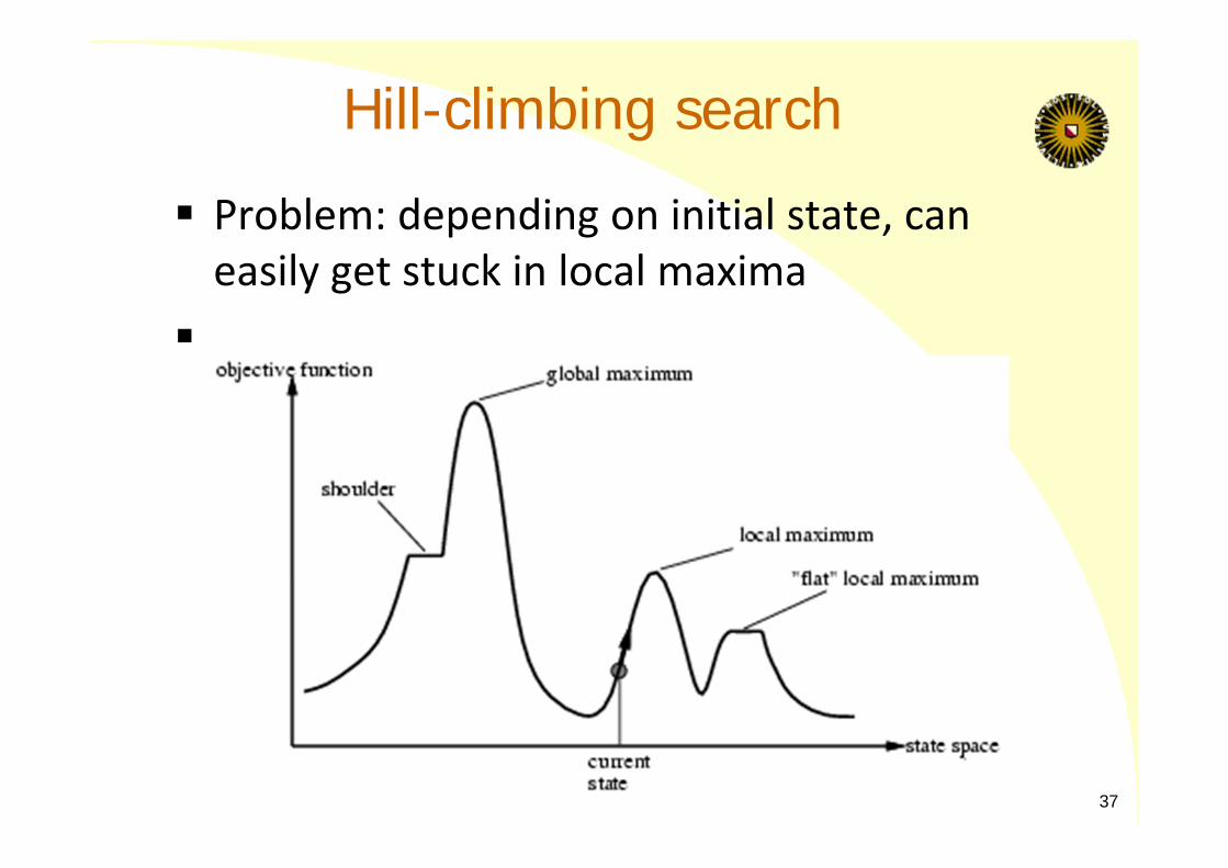
Hill-climbing search
Problem: depending on initial state, can easily get stuck in local maxima
37
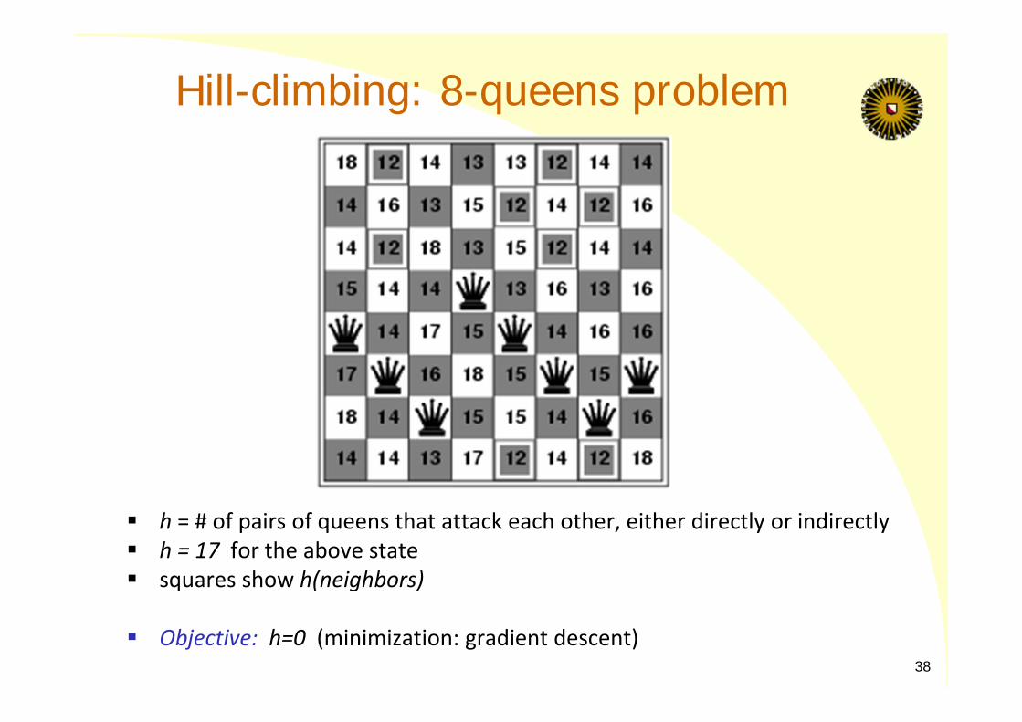
Hill-climbing: 8-queens problem
h = # of pairs of queens that attack each other, either directly or indirectly h = 17 for the above state squares show h(neighbors)
Objective: h=0 (minimization: gradient descent)38
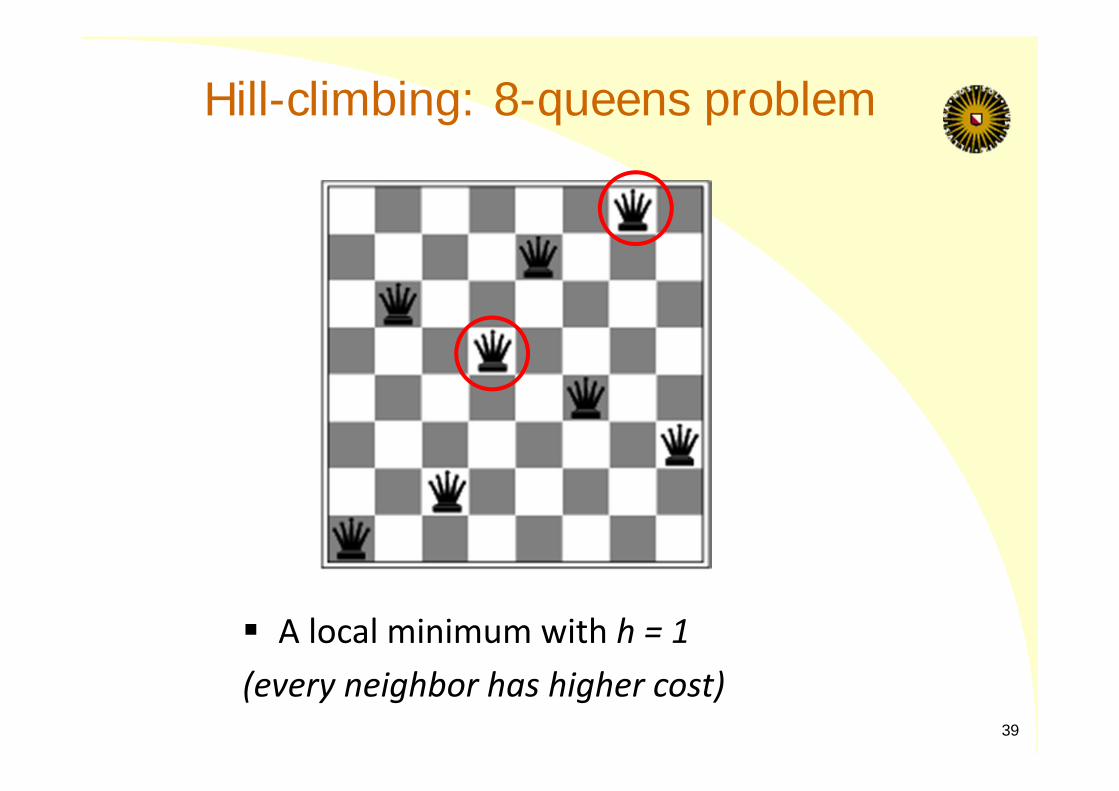
Hill-climbing: 8-queens problem
A local minimum with h = 1(every neighbor has higher cost)
39
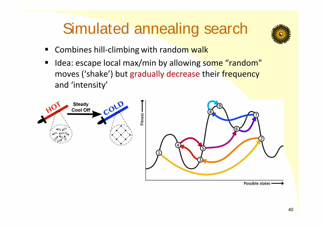
Simulated annealing search Combines hill‐climbingwith random walk Idea: escape local max/min by allowing some “random"
moves (‘shake’) but gradually decrease their frequency and ‘intensity’
40
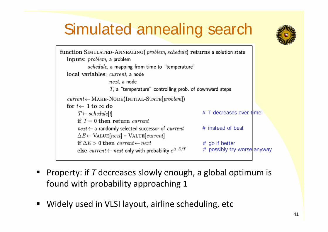
Simulated annealing search
Property: if T decreases slowly enough, a global optimum is found with probability approaching 1
Widely used in VLSI layout, airline scheduling, etc
# instead of best
# possibly try worse anyway
# T decreases over time!
# go if better
41
Local beam search
Keep track of k states in memory rather than just one
Start with k randomly generated states
At each iteration, all the successors of all k states are generated
If any one is a goal state, stop; else select the k best successors from the complete list and repeat.
“Come on over here, the grass is greener!”
42
Genetic algorithms
A successor state is generated by combining two parent states
Start with k randomly generated states (population)
A state (or, individual) is represented as a string over a finite alphabet (often a string of 0s and 1s)
Objective function (or, fitness function): higher values for better states.
Produce the next generation of states by selection, crossover, and mutation
43
Summary Informed Search
Use domain knowledge to guide search towards goal. If path to goal is relevant:
– best first search
If only finding the goal is relevant: – local search