46
Artificial Intelligence Information Systems and Machine Learning Lab (ISMLL) Tomáš Horváth 10 rd November, 2010

Artificial Intelligence
Information Systems and Machine Learning Lab (ISMLL)Tomáš Horváth
10rd November, 2010

Informed Search and Exploration

Example (again)

Informed strategy
● we use a problem-specific knowledge beyond the definition of a problem itself
● evaluation function f(n)● the node with the lowest f(n) will be selected first● BEST-FIRST search
● heuristic function h(n)● the estimated cost of the cheapest path from the
node n to a goal node● somehow imparts an additional knowledge● if n is a goal node, then h(n) = 0

An example heuristic function

Greedy best-first search
● expand the node that is closest to the goal● f(n) = h(n)
● After seeing an example, try to answer● Is this search optimal?● What are the drawbacks?● What complexity does it have?

Greedy best-first search

A* search
● f(n) = g(n) + h(n)● cost for reach the node + cost to get to the goal● estimated cost of the cheapest solution through n
● admissible heuristic h(n)● never overestimates the cost to reach the goal● Is the straight-line distance admissible?
● A* is optimal● if it is used with TREE-SEARCH and● if h(n) is admissible
– How can it be proved?
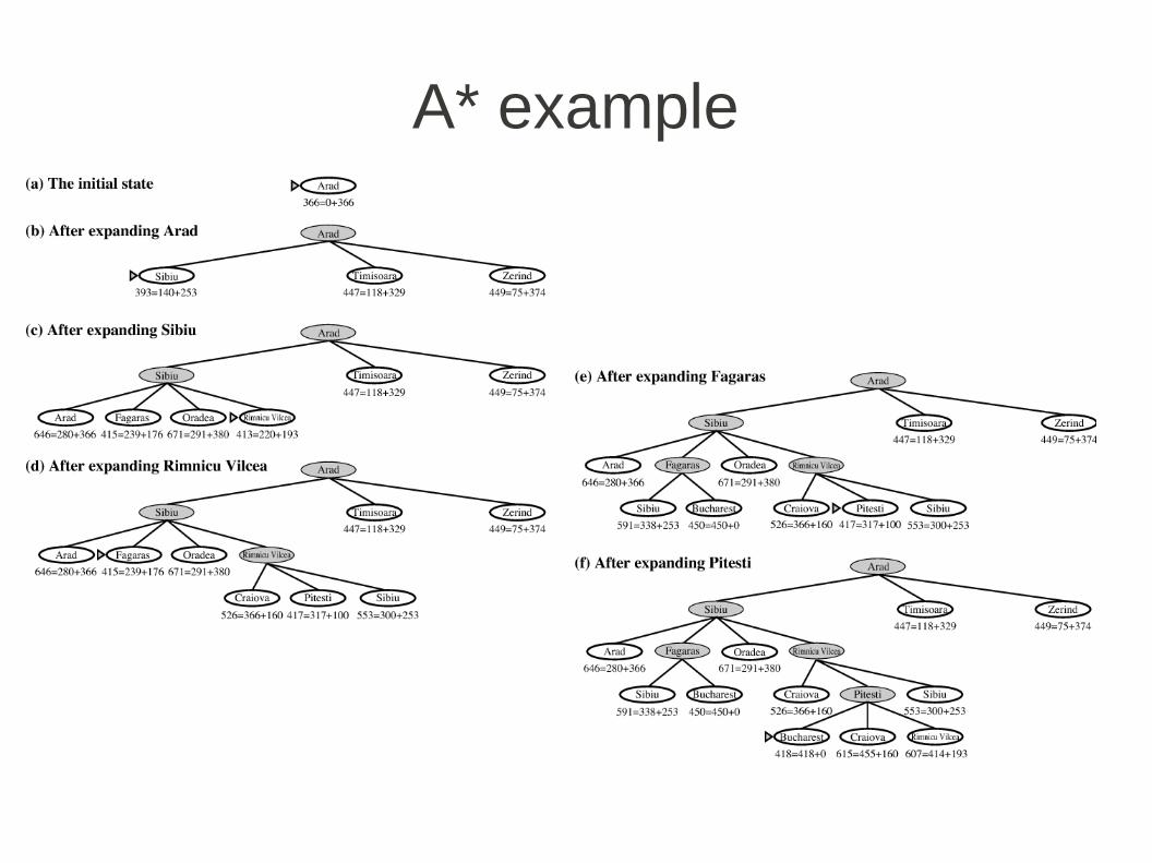
A* example

A* proof (tree-search)
● since g(n) is the exact cost and h(n) is admissible, f(n) never overestimates
● suboptimal goal G2, cost C* for optimal solution● h(G2) = 0
– f(G2) = g(G2) + h(G2) = g(G2) > C*
● consider a node n on an optimal path● if a solution exists, n exists too● h(n) does not overestimate
– f(n) = g(n) + h(n) <= C*● f(n) <= C* < f(G2)
– G2 will not be expanded and A* must return an optimal solution
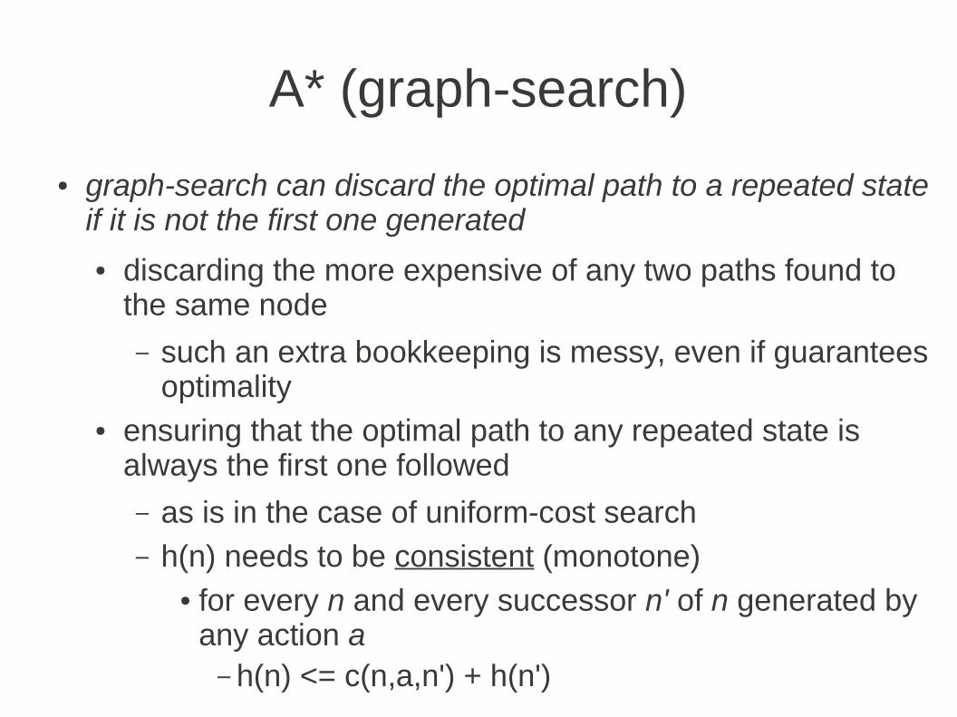
A* (graph-search)
● graph-search can discard the optimal path to a repeated state if it is not the first one generated
● discarding the more expensive of any two paths found to the same node
– such an extra bookkeeping is messy, even if guarantees optimality
● ensuring that the optimal path to any repeated state is always the first one followed
– as is in the case of uniform-cost search– h(n) needs to be consistent (monotone)
● for every n and every successor n' of n generated by any action a– h(n) <= c(n,a,n') + h(n')

A* (graph-search)
● n, n' and the closest goal to n form a triangle
● every consistent heuristic is also admissible● if h(n) is consistent then the values of f(n) along any path are
nondecreasing
● g(n') = g(n) + c(n,a,n')● h(n) <= c(n,a,n') + h(n')
– f(n') = g(n') + h(n') = g(n) + c(n,a,n') + h(n') >= g(n) + h(n) = f(n)
● A* using graph-search is optimal if h(n) is consistent
● sequence of nodes expanded by A* using graph-search is in nondecreasing order of f(n)
– the first goal node selected for expansion must be optimal since all later nodes will be at least as expensive

A* - contoursuniform cost search: h(n) = 0

A* - large-scale problems
● expand no nodes with f(n) > C*● such nodes are pruned
● however, the number of nodes within the goal contour is for most problems still exponential● unless |h(n) – h*(n)| <= O(log h*(n))
– h*(n) is the true cost of getting from n to the goal● impractical to insist on finding an optimal solution
– variants of A* for finding suboptimal solutions quickly● keeps all generated nodes in the memory
– as all graph-search algorithms

Memory-bounded heuristic search
● we can simply adapt the idea of iterative-deepening (IDA*)● use the smallest f-cost of any node that exceeded
the cutoff in the previous iteration as a new cutoff● practical for problems with unit-step cost● with real-valued costs it suffers from the same
difficulties as does the iterative version of uniform-cost search

Recursive best-first search
● a simple recursive algorithm but● it keeps track of the f-value of the best alternative
path available from any ancestor of the current node● if the current node exceeds the limit the recursion
unwinds back to the alternative path– replaces the f-value of each node along the path with the
best f-value of its children
● remembers the f-value of the best leaf in the forgotten subtree

Recursive best-first search

Recursive best-first search

IDA* and RBFS
● like A*, is optimal if h(n) is admissible● excessive node regeneration● space complexity is linear in depth of the
deepest optimal solution● hard to characterize it's time complexity
● they may explore the same state many times
● IDA* and RBFS suffers from too little memory● it seems sensible to use all available memory

Simplified memory-bounded A*
● proceeds like A* until the memory is full● if the memory is full SMA* drops the worst leaf
node (with the highest value)● SMA* regenerates the subtree only when all
other paths have been shown to look worse than the path it has forgotten
● What if all the leaf nodes have the same value?
● SMA* is complete if the depth of the shallowest goal is less than the memory size
● extra time needed for repeated regeneration
A short note on heuristics
● 8-puzzle example● h1 = the number of misplaced tiles● h2 = the sum of the distances of the tiles from their goal
position (Manhattan distance)● Which one is better?
● effective branching factor● that a uniform tree of depth d would have when
containing N+1 total nodes generated● N+1 = 1 + b* + b*^2 + … + b*^d● a well-designed heuristic would have b* close to 1

A short note on heuristics
● h2 is better than h1 for an 8-puzzle problem● Is it always better?
● h2 dominates h1● if for any node n, h2(n) >= h1(n)
– using h2 will never expand more nodes than h1● every node with f(n) < C* will surely be expanded● every node with h(n) < C* - g(n) will surely be expanded● since h2 is at least as big as h1 for all nodes, every node surely
expanded with h2 will also be surely expanded with h1
● it is always better to use heuristic with higher values– just if the heuristic does not overestimate
Local search and Optimization
● sometimes the path to the goal is irrelevant● e.g. 8-queen
● Local search algorithms● not systematic
– use a single current state– generally, move only to neighbors– typically, the paths are not retained
● use very little memory● often find reasonable solutions in large spaces
● Optimization problems● find the best state according to an objective function

Hill-climbing search
● What are the drawbacks of this algorithm?

Hill-climbing search

Hill-climbing search
● Sideways moves● allow when a plateau is reached
Hill-climbing search
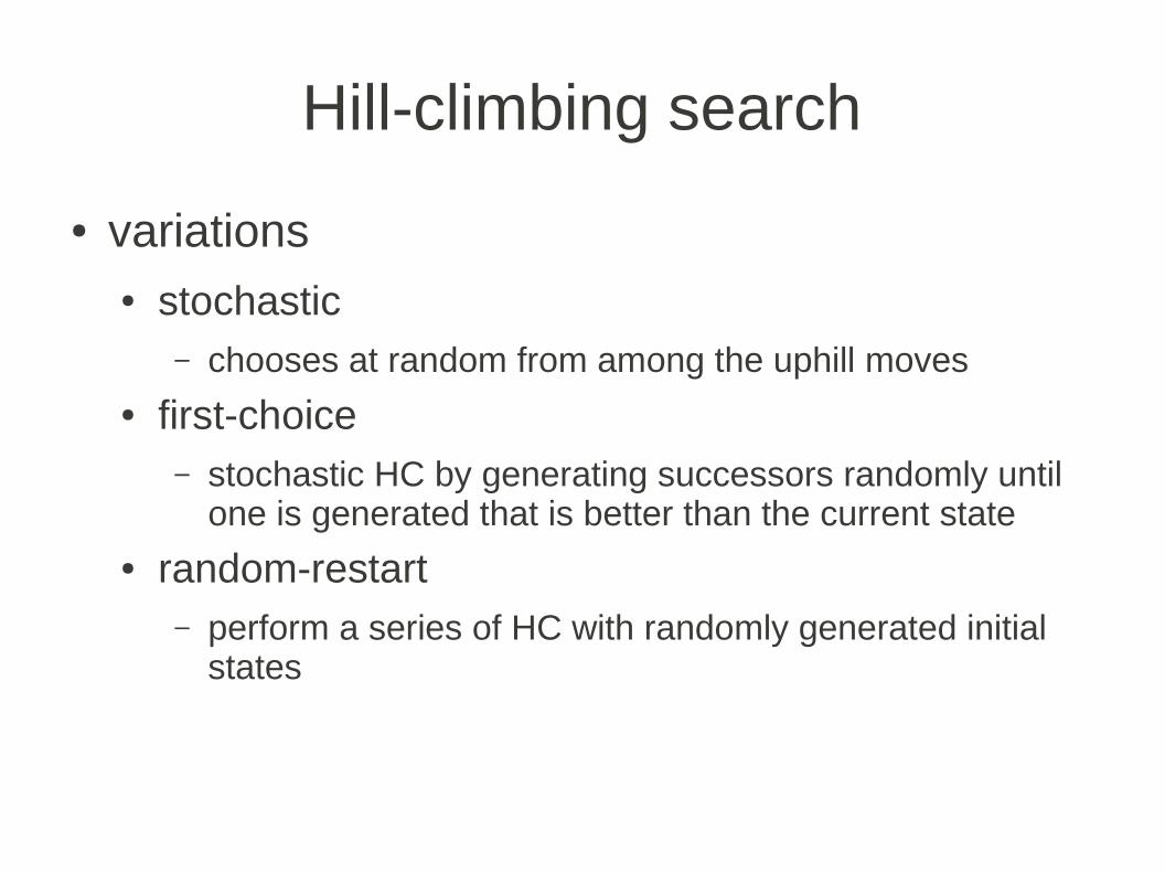
● variations● stochastic
– chooses at random from among the uphill moves● first-choice
– stochastic HC by generating successors randomly until one is generated that is better than the current state
● random-restart– perform a series of HC with randomly generated initial
states

Simulated Annealing
● HC never makes “downhill” move● it can stuck in the local maximum
● random-walk● is inefficient
● it seems reasonable to combine HC and RW● simulated annealing
– motivated by a process of annealing in metallurgy
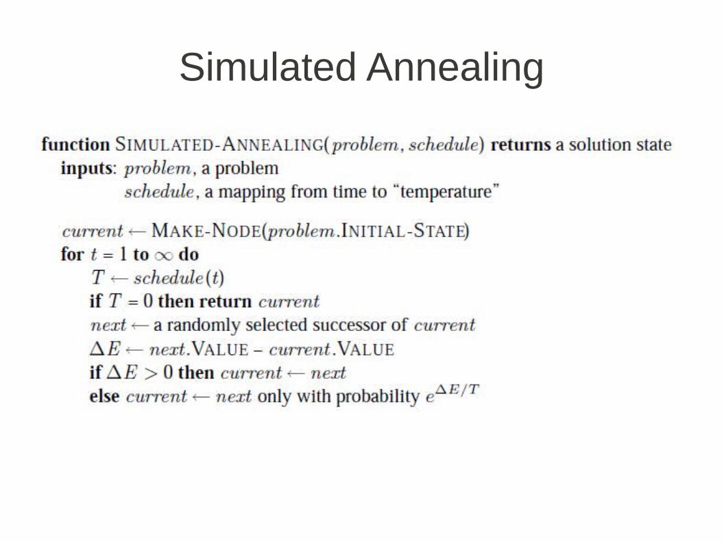
Simulated Annealing
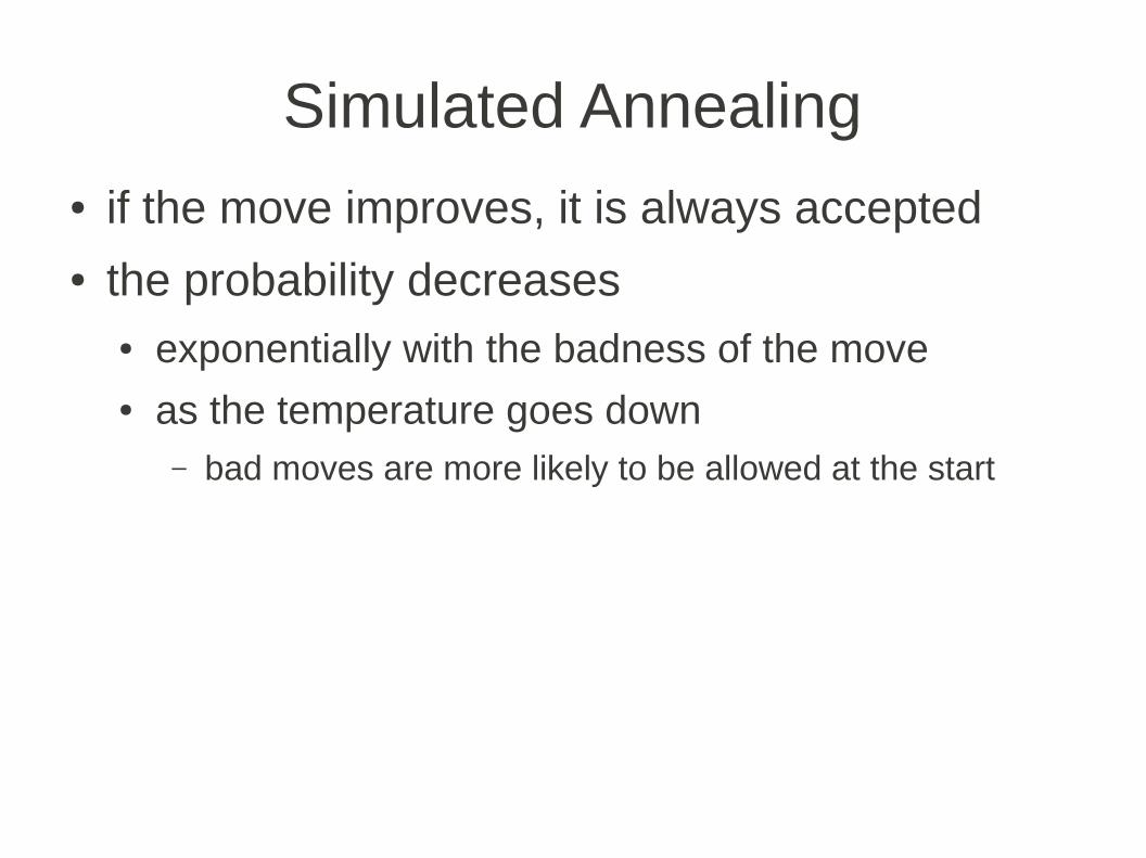
Simulated Annealing● if the move improves, it is always accepted● the probability decreases
● exponentially with the badness of the move● as the temperature goes down
– bad moves are more likely to be allowed at the start
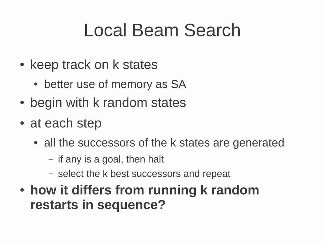
Local Beam Search
● keep track on k states● better use of memory as SA
● begin with k random states● at each step
● all the successors of the k states are generated– if any is a goal, then halt– select the k best successors and repeat
● how it differs from running k random restarts in sequence?

Local Beam Search
● useful information is passed among the k parallel search threads● e.g. 1 state generates several good successors while
other states generates bad successors● moves the resources to prospective areas of the
search space
● the k successors can quickly become concentrated in a small area of the space● stochastic beam search
– the probability of choosing a successor grows with its value● a “natural” selection
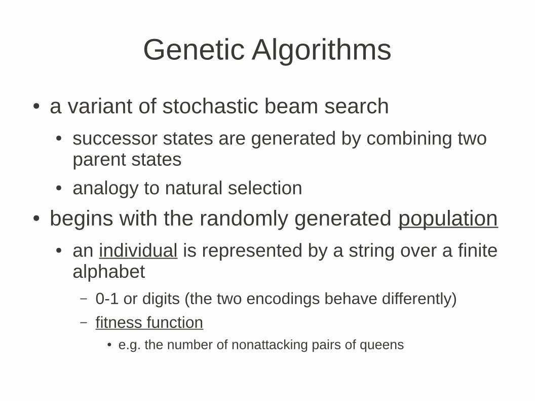
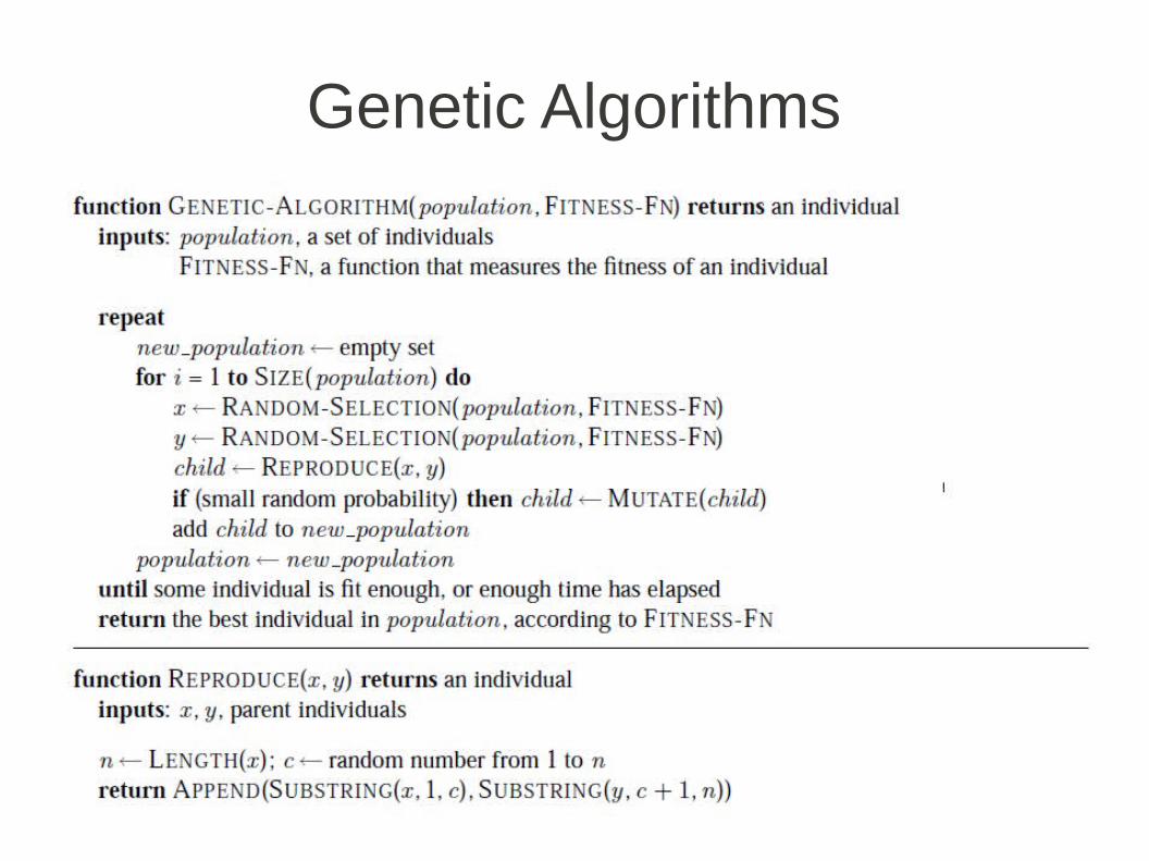
Genetic Algorithms
● a variant of stochastic beam search● successor states are generated by combining two
parent states● analogy to natural selection
● begins with the randomly generated population● an individual is represented by a string over a finite
alphabet– 0-1 or digits (the two encodings behave differently)– fitness function
● e.g. the number of nonattacking pairs of queens

Genetic Algorithms
Genetic Algorithms

Genetic Algorithms
● the crossover operation has the ability to combine large blocks● doing crossover in a random order, however, makes
no advantage● schema
– for example 246*****– instances of the schema– makes sense, if adjacent bits are related each other, i.e.
when schemas correspond to meaningful components of a solution

Local search in continuous spaces
● example - we have to put 3 airports on the map● sum of squared distances from each city to the
closest airport is minimized● coordinates (x1,y1), (x2,y2), (x3,y3)
– six variables– objective function f(x1,y1,x2,y2,x3,y3) is tricky to express– how could we apply e.g. hill climbing?
● can we discretize the neighborhood of the states (+- delta)?

Local search in continuous spaces
● gradient ascent algorithms● ▽f = (∂f/∂x1,∂f/∂y1,∂f/∂x2,∂f/∂y2,∂f/∂x3,∂f/∂y3)
– we can compute the gradient only locally● perform steepest-ascent hill climbing
– x_new = x_old + α f(x)▽– α is a “small” constant
● if too small, many steps are needed● if too large, it can overshoot the maximum
– line search● doubling α until f starts to decrease● this point becames the new state
– α
Local search in continuous spaces
● sometimes an objective function is not available in a differentiable form
– for example is computed by some other (external) tools– in this case use empirical gradient
● evaluating the response to small increments and decrements in each coordinate
● several variations of the gradient ascent algorithm

On-line search
● can be solved only by an agent executing actions rather than by a purely computational process
● an agent knows just● ACTION(s)● c(s,a,s')● GOAL_TEST(s)
● an agent can expand
only the node that it
physically occupies!

On-line DFS agent
Random Walk
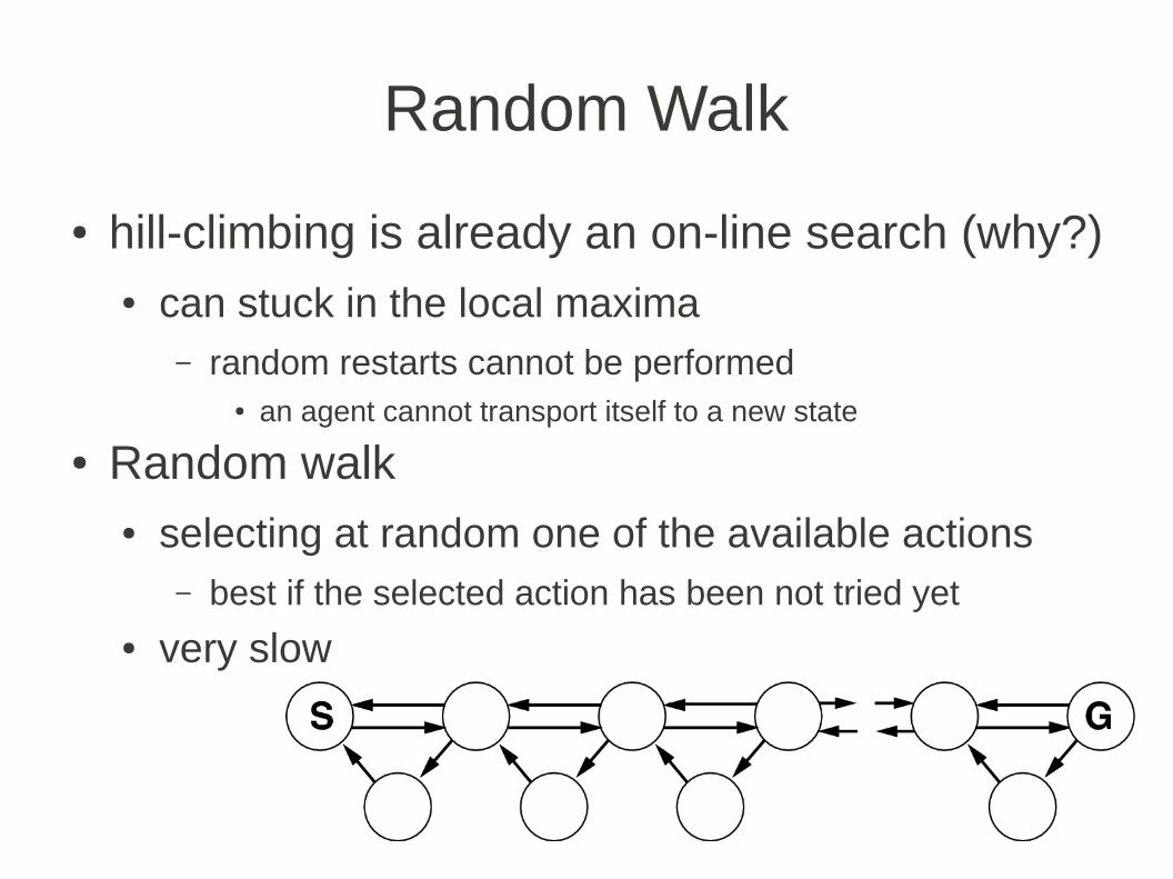
● hill-climbing is already an on-line search (why?)● can stuck in the local maxima
– random restarts cannot be performed● an agent cannot transport itself to a new state
● Random walk● selecting at random one of the available actions
– best if the selected action has been not tried yet● very slow

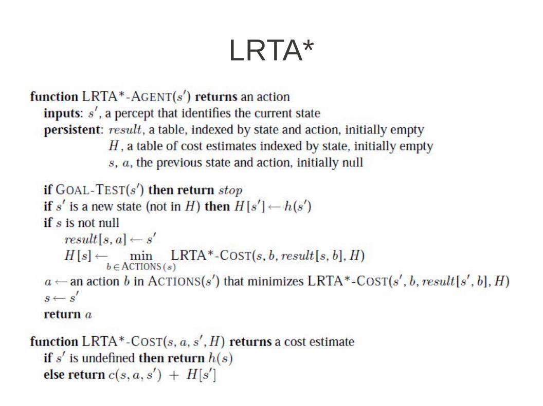
LRTA*
● augmenting HC with memory rather than randomness● store the current estimate H(s) of the cost to reach
the goal from each state that has been visited

LRTA*
LRTA*

Thanks for your attention!Questions?


