Artificial Lift: Making Your Electrical Submersible Pumps...

Artificial Lift: Making Your Electrical Submersible Pumps Talk To You

AuthorSandy Williams, Director, Artificial Lift Performance Ltd

Disclaimer:Whilst every effort has been made to ensure the accuracy of the information contained in this publication, neither Offshore Network Ltd nor any of its affiliates past, present or future warrants its accuracy or will, regardless of its or their negligence, assume liability for any foreseeable or unforeseeable use made thereof, which liability is hereby excluded. Consequently, such use is at the recipient’s own risk on the basis that any use by the recipient constitutes agreement to the terms of this disclaimer. The recipient is obliged to inform any subsequent recipient of such terms. Any reproduction, distribution or public use of this report requires prior written permission from Offshore Network Ltd.

Offshore Network Limited, Registered in England and Wales, Company Registered Number 8702032

Distributed by:Report by:

PAGE 2Offshore Network Limited, Registered in England and Wales, Company Registered Number 8702032


ABSTRACTUsing a diagnostic technique incorporating the use of a gradient traverse plot combined with basic

physics and validation principles, this paper will show how an Electrical Submersible Pump (ESP) can

be designed, installed and operated to increase reliability and extend run-life.

Since interactions between the wellbore and an ESP are complex, a method is required to assist

in the analysis of such interactions. Case histories will demonstrate application of the technique

and highlight the practical benefits where well intervention is costly and must be eliminated or

minimised.

Our industry understands how to design, commission and operate surface pumps to attain reliability.

By applying the same laws of physics and increasing our understanding of ESP performance we can

improve ESP reliability. A discussion of the Gradient Traverse plot analysis technique will highlight

the hierarchy of measured parameters (pressures, temperatures, amps etc) and show how these

parameters can be used to validate well and ESP performance. The technique will then be applied to

interpret complex examples of ESP operating problems and demonstrate how measured parameters

can be used to understand the ESP and well interactions and prevent ESP failures.

This technique facilitates a ‘holistic’ approach to the design, performance monitoring and failure

analysis of an ESP as a system. Consideration of all aspects of well design (well inflow, fluid

properties, completion design, desired rates, cost) is critical to understanding the operating

environment of an ESP. By implementing a technique that allows validation of well and reservoir data

and ESP performance, a better understanding of the system is developed and ‘fit for purpose’ design

can be implemented resulting in a more reliable system, thereby reducing well intervention costs.

INTRODUCTIONThe subject of this paper is ‘a technique to make your ESP talk to you’; when designing and

operating ESPs the first thing that you need to do is give the ESP a ‘mouth’, then you can attempt to

understand its language and let it talk to you.

Traditionally, the ESP ‘mouth’ was an amp chart and a fluid level shot on the annulus. Interpretation

of the data then told you something about motor load and pump intake pressure. Today’s ESP

technology is such that the prudent operator can obtain ESP operating parameters by using a

downhole sensor. The dilemma when faced with the wealth of data that comes from such a sensor

is ‘which parameters are most important?’. By recognising which variables respond most quickly to a

change in operating conditions, you can give your ESP the ability to talk to you.

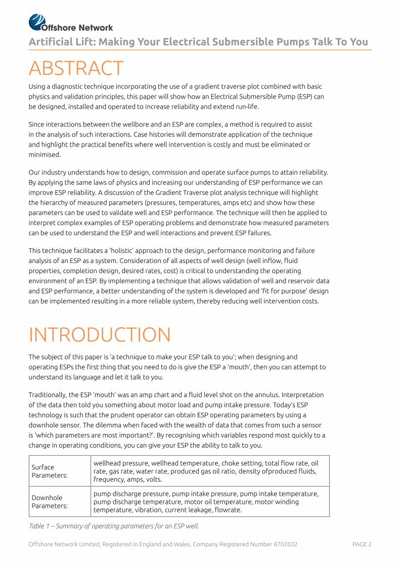
Table 1 – Summary of operating parameters for an ESP well.

SurfaceParameters:

wellhead pressure, wellhead temperature, choke setting, total flow rate, oil rate, gas rate, water rate, produced gas oil ratio, density ofproduced fluids, frequency, amps, volts.

DownholeParameters:

pump discharge pressure, pump intake pressure, pump intake temperature, pump discharge temperature, motor oil temperature, motor winding temperature, vibration, current leakage, flowrate.



Table 1 identifies some of the parameters that an operator may routinely collect on an ESP well.

To focus on which parameters are the most important, the purpose of the ESP needs to be

recognised - to assist a well to produce fluid (hopefully oil) to surface. As such, the ESP should be

considered a part of the well system rather than a pump in isolation. Flow occurs in the well as a

result of reservoir drawdown; an ESP assists the well to flow (or to flow at higher rates) by increasing

the drawdown. Consequently, a change in well behaviour will manifest itself as a pressure change in

the wellbore. This paper will show how pressure information from a downhole sensor on an ESP can

be used to match and diagnose well and ESP performance.

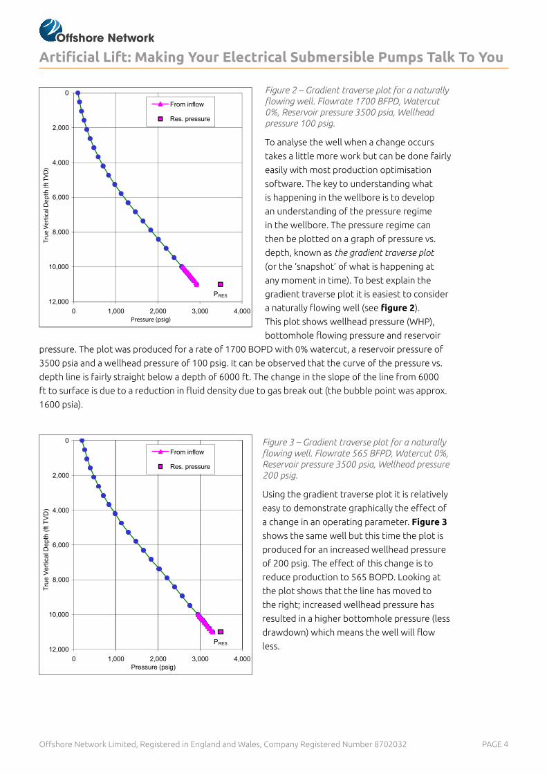
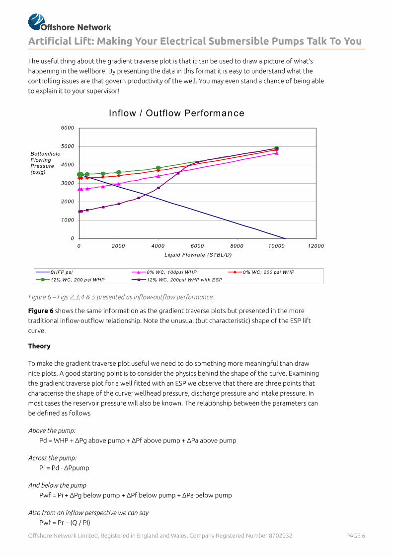
THE TECHNIQUEThe technique utilises the gradient traverse plot to present wellbore pressure and depth information

in a format that makes it easy to grasp the controlling factors in a well. By combining well inflow and

the physics of fluid dynamics it is possible to understand the theory behind the shape of the gradient

traverse plot. The theory can then be applied as part of a step-by-step process to validate ESP

performance, well information and reservoir data.

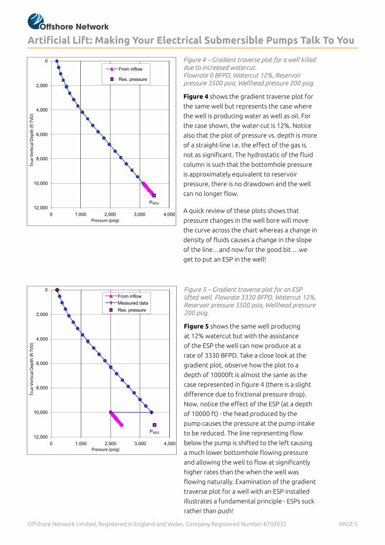
The Gradient Traverse Plot

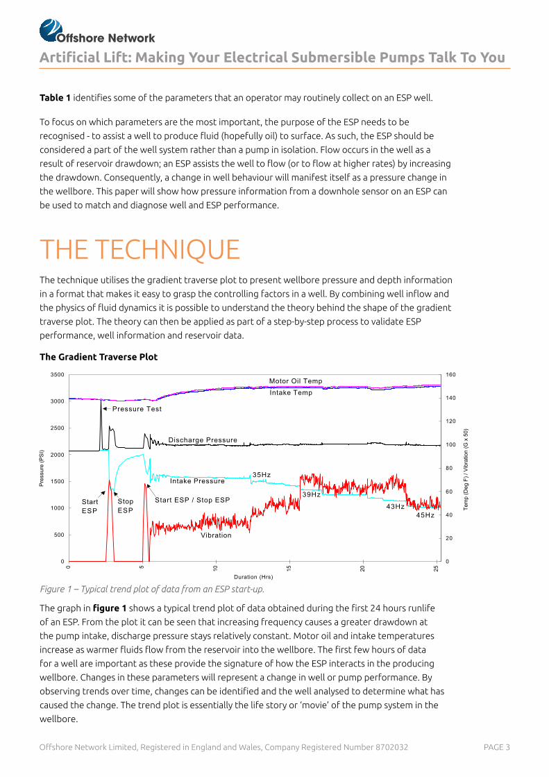
Figure 1 – Typical trend plot of data from an ESP start-up.

The graph in figure 1 shows a typical trend plot of data obtained during the first 24 hours runlife

of an ESP. From the plot it can be seen that increasing frequency causes a greater drawdown at

the pump intake, discharge pressure stays relatively constant. Motor oil and intake temperatures

increase as warmer fluids flow from the reservoir into the wellbore. The first few hours of data

for a well are important as these provide the signature of how the ESP interacts in the producing

wellbore. Changes in these parameters will represent a change in well or pump performance. By

observing trends over time, changes can be identified and the well analysed to determine what has

caused the change. The trend plot is essentially the life story or ‘movie’ of the pump system in the

wellbore.



Figure 2 – Gradient traverse plot for a naturally flowing well. Flowrate 1700 BFPD, Watercut 0%, Reservoir pressure 3500 psia, Wellhead pressure 100 psig.

To analyse the well when a change occurs

takes a little more work but can be done fairly

easily with most production optimisation

software. The key to understanding what

is happening in the wellbore is to develop

an understanding of the pressure regime

in the wellbore. The pressure regime can

then be plotted on a graph of pressure vs.

depth, known as the gradient traverse plot

(or the ‘snapshot’ of what is happening at

any moment in time). To best explain the

gradient traverse plot it is easiest to consider

a naturally flowing well (see figure 2).

This plot shows wellhead pressure (WHP),

bottomhole flowing pressure and reservoir

pressure. The plot was produced for a rate of 1700 BOPD with 0% watercut, a reservoir pressure of

3500 psia and a wellhead pressure of 100 psig. It can be observed that the curve of the pressure vs.

depth line is fairly straight below a depth of 6000 ft. The change in the slope of the line from 6000

ft to surface is due to a reduction in fluid density due to gas break out (the bubble point was approx.

1600 psia).

Figure 3 – Gradient traverse plot for a naturally flowing well. Flowrate 565 BFPD, Watercut 0%, Reservoir pressure 3500 psia, Wellhead pressure 200 psig.

Using the gradient traverse plot it is relatively

easy to demonstrate graphically the effect of

a change in an operating parameter. Figure 3

shows the same well but this time the plot is

produced for an increased wellhead pressure

of 200 psig. The effect of this change is to

reduce production to 565 BOPD. Looking at

the plot shows that the line has moved to

the right; increased wellhead pressure has

resulted in a higher bottomhole pressure (less

drawdown) which means the well will flow

less.



Figure 4 – Gradient traverse plot for a well killed due to increased watercut. Flowrate 0 BFPD, Watercut 12%, Reservoir pressure 3500 psia, Wellhead pressure 200 psig.

Figure 4 shows the gradient traverse plot for

the same well but represents the case where

the well is producing water as well as oil. For

the case shown, the water-cut is 12%. Notice

also that the plot of pressure vs. depth is more

of a straight-line i.e. the effect of the gas is

not as significant. The hydrostatic of the fluid

column is such that the bottomhole pressure

is approximately equivalent to reservoir

pressure, there is no drawdown and the well

can no longer flow.

A quick review of these plots shows that

pressure changes in the well bore will move

the curve across the chart whereas a change in

density of fluids causes a change in the slope

of the line…and now for the good bit …we

get to put an ESP in the well!

Figure 5 – Gradient traverse plot for an ESP lifted well. Flowrate 3330 BFPD, Watercut 12%, Reservoir pressure 3500 psia, Wellhead pressure 200 psig.

Figure 5 shows the same well producing

at 12% watercut but with the assistance

of the ESP the well can now produce at a

rate of 3330 BFPD. Take a close look at the

gradient plot, observe how the plot to a

depth of 10000ft is almost the same as the

case represented in figure 4 (there is a slight

difference due to frictional pressure drop).

Now, notice the effect of the ESP (at a depth

of 10000 ft) - the head produced by the

pump causes the pressure at the pump intake

to be reduced. The line representing flow

below the pump is shifted to the left causing

a much lower bottomhole flowing pressure

and allowing the well to flow at significantly

higher rates than the when the well was

flowing naturally. Examination of the gradient

traverse plot for a well with an ESP installed

illustrates a fundamental principle - ESPs suck

rather than push!



The useful thing about the gradient traverse plot is that it can be used to draw a picture of what’s

happening in the wellbore. By presenting the data in this format it is easy to understand what the

controlling issues are that govern productivity of the well. You may even stand a chance of being able

to explain it to your supervisor!

Figure 6 – Figs 2,3,4 & 5 presented as inflow-outflow performance.

Figure 6 shows the same information as the gradient traverse plots but presented in the more

traditional inflow-outflow relationship. Note the unusual (but characteristic) shape of the ESP lift

curve.

Theory

To make the gradient traverse plot useful we need to do something more meaningful than draw

nice plots. A good starting point is to consider the physics behind the shape of the curve. Examining

the gradient traverse plot for a well fitted with an ESP we observe that there are three points that

characterise the shape of the curve; wellhead pressure, discharge pressure and intake pressure. In

most cases the reservoir pressure will also be known. The relationship between the parameters can

be defined as follows

Above the pump:

Pd = WHP + ∆Pg above pump + ∆Pf above pump + ∆Pa above pump

Across the pump:

Pi = Pd - ∆Ppump

And below the pump

Pwf = Pi + ∆Pg below pump + ∆Pf below pump + ∆Pa below pump

Also from an inflow perspective we can say

Pwf = Pr – (Q / PI)



Where

Pd = discharge pressure (psi)

Pi = intake pressure (psi)

WHP = wellhead pressure (psi)

∆Pg = hydrostatic head (gravity pressure loss in psi)

∆Pf = frictional pressure loss (psi)

∆Pa = acceleration pressure loss (psi)

∆Ppump = (Head in feet x fluid specific gravity/2.31) (psi)

Pwf = bottomhole flowing pressure (psi)

Pr = reservoir pressure (psi)

Q = well flowrate in stock tank barrels liquid (stbl/day)

PI = productivity index (stbl/day/psi)

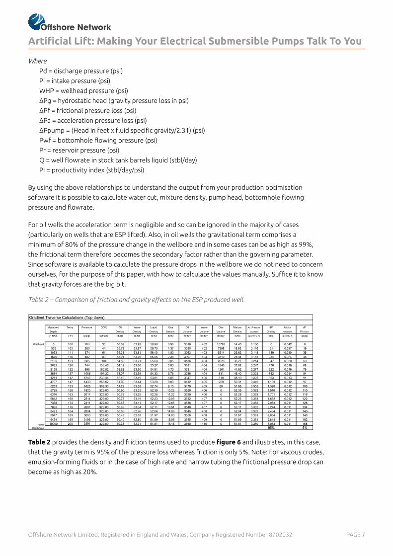
By using the above relationships to understand the output from your production optimisation

software it is possible to calculate water cut, mixture density, pump head, bottomhole flowing

pressure and flowrate.

For oil wells the acceleration term is negligible and so can be ignored in the majority of cases

(particularly on wells that are ESP lifted). Also, in oil wells the gravitational term comprises a

minimum of 80% of the pressure change in the wellbore and in some cases can be as high as 99%,

the frictional term therefore becomes the secondary factor rather than the governing parameter.

Since software is available to calculate the pressure drops in the wellbore we do not need to concern

ourselves, for the purpose of this paper, with how to calculate the values manually. Suffice it to know

that gravity forces are the big bit.

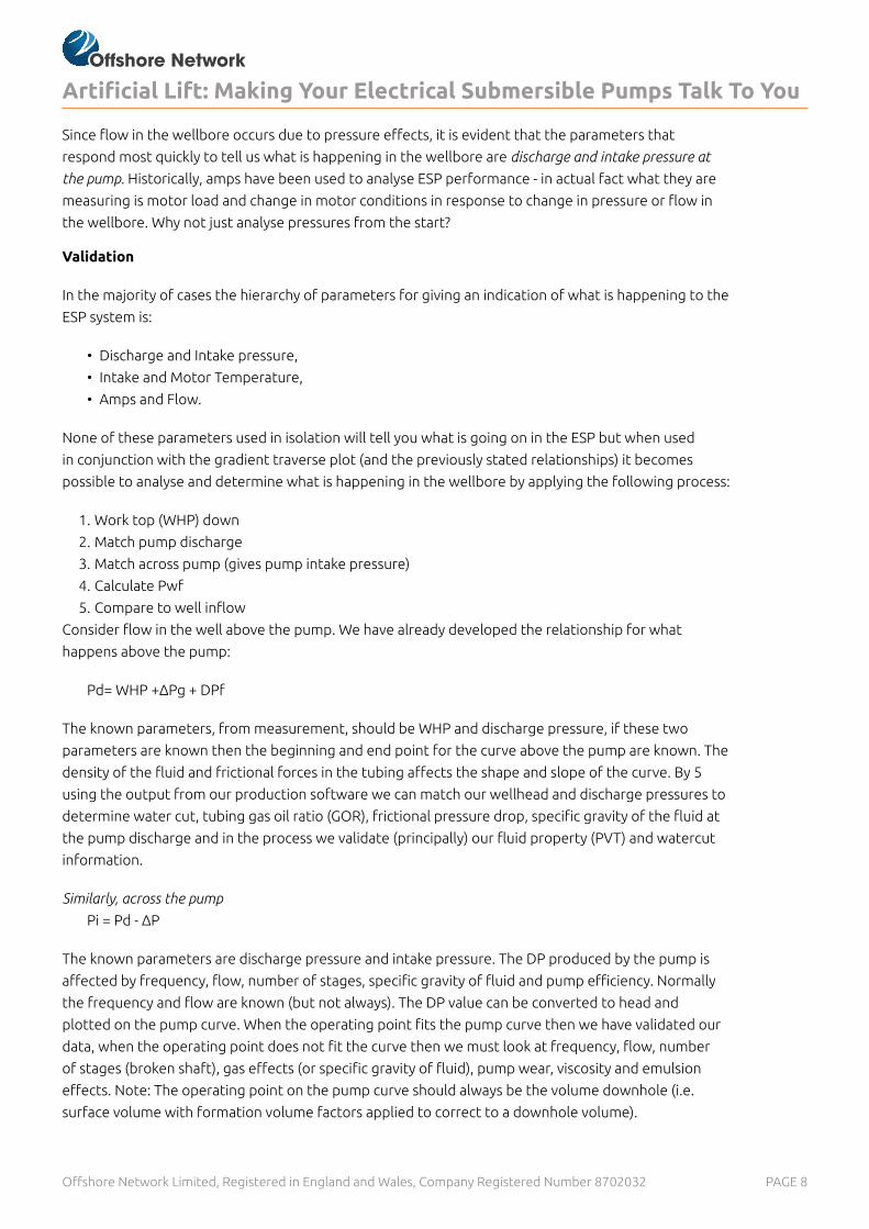
Table 2 – Comparison of friction and gravity effects on the ESP produced well.

Table 2 provides the density and friction terms used to produce figure 6 and illustrates, in this case,

that the gravity term is 95% of the pressure loss whereas friction is only 5%. Note: For viscous crudes,

emulsion-forming fluids or in the case of high rate and narrow tubing the frictional pressure drop can

become as high as 20%.



Since flow in the wellbore occurs due to pressure effects, it is evident that the parameters that

respond most quickly to tell us what is happening in the wellbore are discharge and intake pressure at

the pump. Historically, amps have been used to analyse ESP performance - in actual fact what they are

measuring is motor load and change in motor conditions in response to change in pressure or flow in

the wellbore. Why not just analyse pressures from the start?

Validation

In the majority of cases the hierarchy of parameters for giving an indication of what is happening to the

ESP system is:

• Discharge and Intake pressure,

• Intake and Motor Temperature,

• Amps and Flow.

None of these parameters used in isolation will tell you what is going on in the ESP but when used

in conjunction with the gradient traverse plot (and the previously stated relationships) it becomes

possible to analyse and determine what is happening in the wellbore by applying the following process:

1. Work top (WHP) down

2. Match pump discharge

3. Match across pump (gives pump intake pressure)

4. Calculate Pwf

5. Compare to well inflow

Consider flow in the well above the pump. We have already developed the relationship for what

happens above the pump:

Pd= WHP +∆Pg + DPf

The known parameters, from measurement, should be WHP and discharge pressure, if these two

parameters are known then the beginning and end point for the curve above the pump are known. The

density of the fluid and frictional forces in the tubing affects the shape and slope of the curve. By 5

using the output from our production software we can match our wellhead and discharge pressures to

determine water cut, tubing gas oil ratio (GOR), frictional pressure drop, specific gravity of the fluid at

the pump discharge and in the process we validate (principally) our fluid property (PVT) and watercut

information.

Similarly, across the pump

Pi = Pd - ∆P

The known parameters are discharge pressure and intake pressure. The DP produced by the pump is

affected by frequency, flow, number of stages, specific gravity of fluid and pump efficiency. Normally

the frequency and flow are known (but not always). The DP value can be converted to head and

plotted on the pump curve. When the operating point fits the pump curve then we have validated our

data, when the operating point does not fit the curve then we must look at frequency, flow, number

of stages (broken shaft), gas effects (or specific gravity of fluid), pump wear, viscosity and emulsion

effects. Note: The operating point on the pump curve should always be the volume downhole (i.e.

surface volume with formation volume factors applied to correct to a downhole volume).



And below the pump

Pwf = Pi + ∆Pf + ∆Pg

Since the PVT and watercut should already have been validated above the pump, it should be

straightforward to model down from the pump intake to the reservoir interval and calculate a

bottomhole pressure (note that the friction term below an ESP is usually small due to the larger

casing diameter.) The bottomhole pressure should also correspond with that calculated from the

inflow performance relationship for the given flow rate. Knowledge of the bottomhole pressure

allows you to determine PI or reservoir pressure (one has to be known and the other can be

calculated).

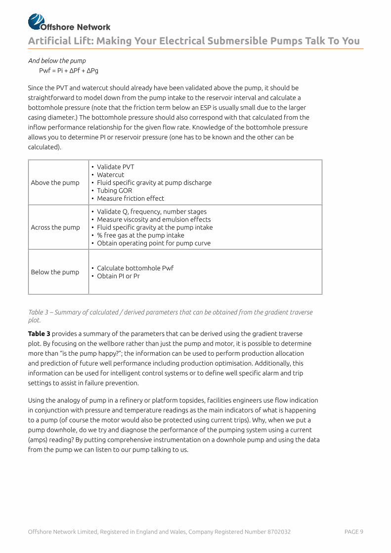
Table 3 – Summary of calculated / derived parameters that can be obtained from the gradient traverse plot.

Table 3 provides a summary of the parameters that can be derived using the gradient traverse

plot. By focusing on the wellbore rather than just the pump and motor, it is possible to determine

more than “is the pump happy?”; the information can be used to perform production allocation

and prediction of future well performance including production optimisation. Additionally, this

information can be used for intelligent control systems or to define well specific alarm and trip

settings to assist in failure prevention.

Using the analogy of pump in a refinery or platform topsides, facilities engineers use flow indication

in conjunction with pressure and temperature readings as the main indicators of what is happening

to a pump (of course the motor would also be protected using current trips). Why, when we put a

pump downhole, do we try and diagnose the performance of the pumping system using a current

(amps) reading? By putting comprehensive instrumentation on a downhole pump and using the data

from the pump we can listen to our pump talking to us.

Above the pump

• Validate PVT• Watercut• Fluid specific gravity at pump discharge• Tubing GOR• Measure friction effect

Across the pump

• Validate Q, frequency, number stages• Measure viscosity and emulsion effects• Fluid specific gravity at the pump intake• % free gas at the pump intake• Obtain operating point for pump curve

Below the pump• Calculate bottomhole Pwf• Obtain PI or Pr



THE APPLICATIONConsideration of the following examples and case histories should help to explain how the technique

is applied in practice to analyse and predict the performance of the well and ESP.

Case 1 - Failure Analysis or Failure Prevention – Your choice!

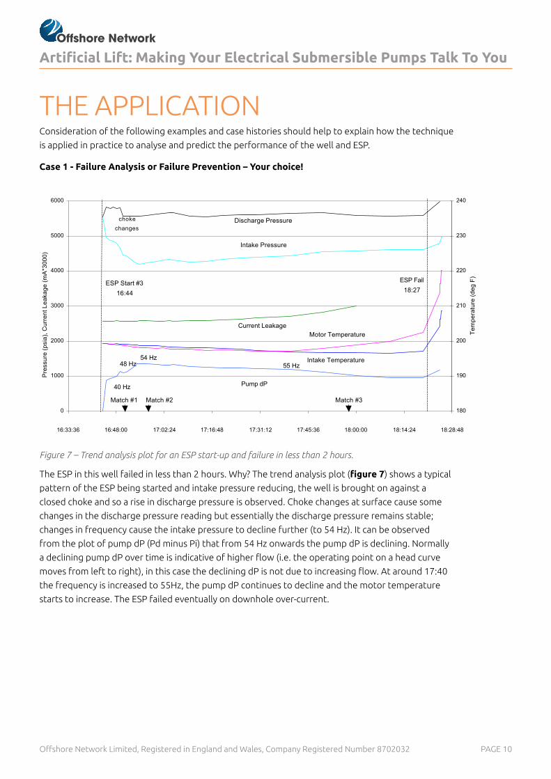
Figure 7 – Trend analysis plot for an ESP start-up and failure in less than 2 hours.

The ESP in this well failed in less than 2 hours. Why? The trend analysis plot (figure 7) shows a typical

pattern of the ESP being started and intake pressure reducing, the well is brought on against a

closed choke and so a rise in discharge pressure is observed. Choke changes at surface cause some

changes in the discharge pressure reading but essentially the discharge pressure remains stable;

changes in frequency cause the intake pressure to decline further (to 54 Hz). It can be observed

from the plot of pump dP (Pd minus Pi) that from 54 Hz onwards the pump dP is declining. Normally

a declining pump dP over time is indicative of higher flow (i.e. the operating point on a head curve

moves from left to right), in this case the declining dP is not due to increasing flow. At around 17:40

the frequency is increased to 55Hz, the pump dP continues to decline and the motor temperature

starts to increase. The ESP failed eventually on downhole over-current.



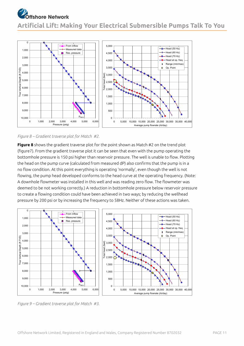
Figure 8 – Gradient traverse plot for Match #2.

Figure 8 shows the gradient traverse plot for the point shown as Match #2 on the trend plot

(figure7). From the gradient traverse plot it can be seen that even with the pump operating the

bottomhole pressure is 150 psi higher than reservoir pressure. The well is unable to flow. Plotting

the head on the pump curve (calculated from measured dP) also confirms that the pump is in a

no flow condition. At this point everything is operating ‘normally’, even though the well is not

flowing, the pump head developed conforms to the head curve at the operating frequency. (Note:

A downhole flowmeter was installed in this well and was reading zero flow. The flowmeter was

deemed to be not working correctly.) A reduction in bottomhole pressure below reservoir pressure

to create a flowing condition could have been achieved in two ways; by reducing the wellhead

pressure by 200 psi or by increasing the frequency to 58Hz. Neither of these actions was taken.




Figure 9 shows the gradient traverse plot shown as Match 3 on the data trend plot after the

frequency had been increased to 55 Hz. The plot shows that the pump head has decreased and no

longer conforms to the expected head curve for the operating frequency indicating damage to the

pump impellers / diffusers. The ESP ran a further 30 minutes before failing on over-current.

At no time during the life of this pump was enough reservoir drawdown achieved to allow the well

to flow; this was the fundamental cause of failure. This analysis was performed as a failure analysis

which could so easily have been failure prevention if the appropriate tools had been used during

startup of the well.

Case 2 – Validation of PVT and PI

This example illustrates the extent of information that can be gained by an analysis of the data

collected from monitoring an ESP system. Apart from diagnosing pump performance, the data has

been used to infer fluid properties, well flowrate, watercut and bottomhole pressure.

This well is a recompletion to an upper reservoir zone. The zone had been tested during a drill stem

test in an offset well as part of the original field discovery. No PVT data existed for this zone. The ESP

system for this well was designed using PVT for the lower reservoir. By using the trend analysis plot

in combination with the gradient traverse plot it was possible to highlight that hydrocarbon (PVT)

properties were very different from those that had been used for the ESP design.

Matching the discharge pressure (above the pump) for a known WHP and watercut proved to be

unsuccessful using the PVT for the lower zone. Validation indicated that to match the discharge

pressure a light but dead oil fluid (32º API) with unusually low GOR

(6 scf/stb) and bubble point (50 psia) would have to be present.

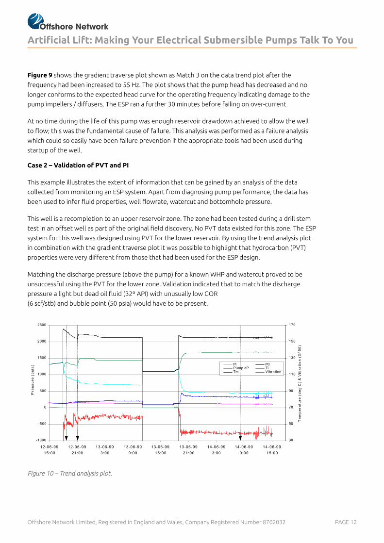
Figure 10 – Trend analysis plot.



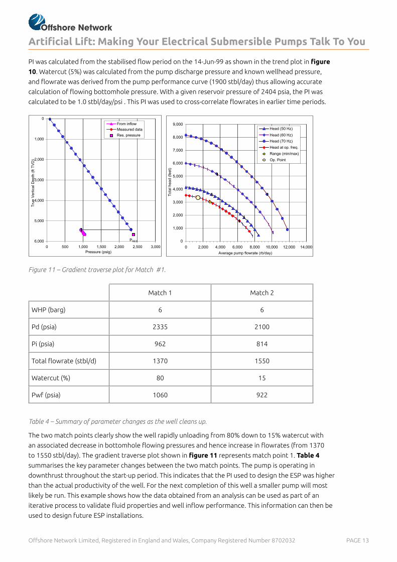
PI was calculated from the stabilised flow period on the 14-Jun-99 as shown in the trend plot in figure

10. Watercut (5%) was calculated from the pump discharge pressure and known wellhead pressure,

and flowrate was derived from the pump performance curve (1900 stbl/day) thus allowing accurate

calculation of flowing bottomhole pressure. With a given reservoir pressure of 2404 psia, the PI was

calculated to be 1.0 stbl/day/psi . This PI was used to cross-correlate flowrates in earlier time periods.


Table 4 – Summary of parameter changes as the well cleans up.

The two match points clearly show the well rapidly unloading from 80% down to 15% watercut with

an associated decrease in bottomhole flowing pressures and hence increase in flowrates (from 1370

to 1550 stbl/day). The gradient traverse plot shown in figure 11 represents match point 1. Table 4

summarises the key parameter changes between the two match points. The pump is operating in

downthrust throughout the start-up period. This indicates that the PI used to design the ESP was higher

than the actual productivity of the well. For the next completion of this well a smaller pump will most

likely be run. This example shows how the data obtained from an analysis can be used as part of an

iterative process to validate fluid properties and well inflow performance. This information can then be

used to design future ESP installations.

Match 1 Match 2

WHP (barg) 6 6

Pd (psia) 2335 2100

Pi (psia) 962 814

Total flowrate (stbl/d) 1370 1550

Watercut (%) 80 15

Pwf (psia) 1060 922



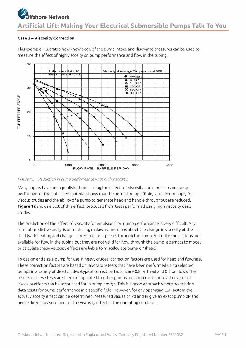
Case 3 – Viscosity Correction

This example illustrates how knowledge of the pump intake and discharge pressures can be used to

measure the effect of high viscosity on pump performance and flow in the tubing.

Figure 12 – Reduction in pump performance with high viscosity.

Many papers have been published concerning the effects of viscosity and emulsions on pump

performance. The published material shows that the normal pump affinity laws do not apply for

viscous crudes and the ability of a pump to generate head and handle throughput are reduced.

Figure 12 shows a plot of this effect, produced from tests performed using high viscosity dead

crudes.

The prediction of the effect of viscosity (or emulsions) on pump performance is very difficult. Any

form of predictive analysis or modelling makes assumptions about the change in viscosity of the

fluid (with heating and change in pressure) as it passes through the pump. Viscosity correlations are

available for flow in the tubing but they are not valid for flow through the pump; attempts to model

or calculate these viscosity effects are liable to miscalculate pump dP (head).

To design and size a pump for use in heavy crudes, correction factors are used for head and flowrate.

These correction factors are based on laboratory tests that have been performed using selected

pumps in a variety of dead crudes (typical correction factors are 0.8 on head and 0.5 on flow). The

results of these tests are then extrapolated to other pumps to assign correction factors so that

viscosity effects can be accounted for in pump design. This is a good approach where no existing

data exists for pump performance in a specific field. However, for any operating ESP system the

actual viscosity effect can be determined. Measured values of Pd and Pi give an exact pump dP and

hence direct measurement of the viscosity effect at the operating condition.



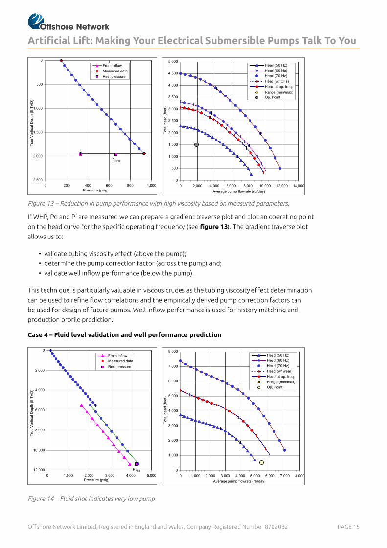
Figure 13 – Reduction in pump performance with high viscosity based on measured parameters.

If WHP, Pd and Pi are measured we can prepare a gradient traverse plot and plot an operating point

on the head curve for the specific operating frequency (see figure 13). The gradient traverse plot

allows us to:

• validate tubing viscosity effect (above the pump);

• determine the pump correction factor (across the pump) and;

• validate well inflow performance (below the pump).

This technique is particularly valuable in viscous crudes as the tubing viscosity effect determination

can be used to refine flow correlations and the empirically derived pump correction factors can

be used for design of future pumps. Well inflow performance is used for history matching and

production profile prediction.

Case 4 – Fluid level validation and well performance prediction

Figure 14 – Fluid shot indicates very low pump



In many land operations where ESPs are relatively inexpensive and can be worked over easily, no

sensors are run downhole. Operators analyse such wells by performing a fluid level measurement

and converting fluid level to pump intake pressure. In this case, the gradient traverse plot was used

to validate well performance data and determine that the fluid level measurement was in error.

The well was known to be producing approx. 5000 stbl/d with a watercut of 54% operating at a

wellhead pressure of 160 psi. The pump installed in the well was direct on line and operating at a

frequency of 60Hz. The indicated bottomhole pressure from a fluid level measurement was 2100

psig. Using production optimisation software the discharge pressure was calculated to be 2306 psig

based on well PVT, watercut and WHP. Plotting this information on the gradient traverse plot (figure

14) shows a very low pump dP (200 psi). This would only be possible if either the flowrate is 30%

higher or the pump is damaged (30% effective stages) and well PI is wrong. One of the initial input

measurements has to be incorrect!

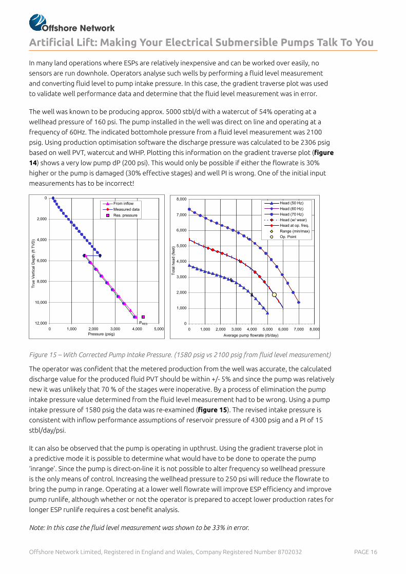
Figure 15 – With Corrected Pump Intake Pressure. (1580 psig vs 2100 psig from fluid level measurement)

The operator was confident that the metered production from the well was accurate, the calculated

discharge value for the produced fluid PVT should be within +/- 5% and since the pump was relatively

new it was unlikely that 70 % of the stages were inoperative. By a process of elimination the pump

intake pressure value determined from the fluid level measurement had to be wrong. Using a pump

intake pressure of 1580 psig the data was re-examined (figure 15). The revised intake pressure is

consistent with inflow performance assumptions of reservoir pressure of 4300 psig and a PI of 15

stbl/day/psi.

It can also be observed that the pump is operating in upthrust. Using the gradient traverse plot in

a predictive mode it is possible to determine what would have to be done to operate the pump

‘inrange’. Since the pump is direct-on-line it is not possible to alter frequency so wellhead pressure

is the only means of control. Increasing the wellhead pressure to 250 psi will reduce the flowrate to

bring the pump in range. Operating at a lower well flowrate will improve ESP efficiency and improve

pump runlife, although whether or not the operator is prepared to accept lower production rates for

longer ESP runlife requires a cost benefit analysis.

Note: In this case the fluid level measurement was shown to be 33% in error.



Case 5 – Production Allocation

Measured parameters can be used throughout the life of the ESP to derive watercut, flowrate,

bottomhole flowing pressure and well productivity index (or reservoir pressure) to assist with

production allocation and reservoir management.

The technique was applied to a well where it was not possible to perform well tests on a regular

basis. By using measured values for WHP, Pi, Pd and frequency, derived values were obtained

for watercut, flowrate, Pwf and PI. Table 5 tabulates the derived parameters for this well and

shows how the technique was used to monitor well clean-up following a workover and to provide

production allocation information for a 6-month period after the watercut had stabilised.

Table 5 - An example of production allocation using measured parameters.



BENEFITS / CONCLUSIONSIn the above examples an attempt has been made to focus on understanding ‘normal’ ESP

performance and how being able to understand what is happening can prevent failures, determine

what is occurring in the wellbore (reservoir, pump, tubing), provide information for ESP design and

aid control and operation of the system. None of these examples used amps to perform diagnosis;

the wells were analysed purely from a hydraulic standpoint (although amps should be used to verify

that the electrical indications match the hydraulic interpretation).

The key to using this technique is to understand what is happening in your well when you first turn

on your ESP. By understanding present and past performance we can quickly identify and analyse

any change in performance. Using this same technique it is possible to diagnose problems such as

plugging at the pump intake, gas locking, tubing leaks, broken pump shafts, pump wear or wrong

PVT (design information). Additionally the method can be extended to predict future well behaviour

based on sensitivity type analyses for watercut, GOR or reservoir pressure.

Understanding your wellbore from a holistic standpoint can help prevent premature ESP failure (as

shown in case 1), be used to set appropriate alarms and trips on ESP control and protection systems

(calculated specifically for each well) and gives the operator the tools to improve pump runlife.

This technique is inexpensive to implement and does not require any new equipment, software

or tools. It simply requires a little education and an understanding of which parameters tell us the

most about what is happening in a well. Most operators already collect the data required to perform

this type of interpretation. In many cases so much data is being collected that people do not know

where to begin analysing the data. This paper identifies the parameters and the technique that

should be your starting point in attempting to understand well performance in ESP lifted (and other

forms of artificial lift) wells. In essence this technique is no different from traditional nodal analysis

techniques, the difference is that the way the information is presented is easy to understand. With

a little practice you too can use this technique to let your ESP talk to you ……..Are you prepared to

listen?


OFFSHORE NETWORK WOULD LOVE TO HEAR FROM YOU…

Offshore Network Ltd. is an independent business intelligence & conference provider catering specifically to the

offshore oil & gas industry. We exist to facilitate a safe and efficient future for the exploration and production of

oil & gas around the globe. We do this by uniting the most influential figures in the industry to challenge the status

quo and share cutting edge innovations. This all happens at our industry leading conferences and through our

original content.

If you would like to contribute to this discussion or are interested in taking part in a future Q&A or article,

please contact Offshore Network today:

[email protected]

www.offsnet.com

UK Telephone: (0)203 411 9937

US Telephone: 713-5706-576

Join the Offshore Engineering Group on LinkedIn

Follow Offshore Network on Twitter

BIOGRAPHY:SANDY WILLIAMSSandy Williams has worked in the Petroleum Industry for 24 years. He is the founder of Artificial Lift

Performance Ltd (ALP), a company which specializes in helping operators get more oil - a skill which

he explains to the layman as being ‘like Viagra for oil wells’.

Sandy worked 9 years for Amoco, then Phoenix and Schlumberger Artificial Lift before becoming

a consultant focused on artificial lift and production optimization. He has worked and lived in the

USA, Oman, Venezuela, Ecuador, Colombia and has taught over 150 courses related to production

optimization and artificial lift and is fluent in Spanish.

He started ALP 10 years ago, a company focused on assisting operators: improve the application of

artificial lift; reduce productions costs and; increase staff competency. ALP also offers a number of

software products to help operators manage artificial lift. ALP is currently assisting operators on

projects in the UK North Sea, Colombia, Oman, Qatar and the USA.

http://www.linkedin.com/groups/Offshore-Engineering-1559757%3Ftrk%3Dmy_groups-b-grp-v

https://www.linkedin.com/groups?home=&gid=1559757&trk=anet_ug_hm&goback=%2Egmr_1559757

https://twitter.com/OffshoreNetwork

Date post:	30-Jun-2018
Category:	Documents
Upload:	hoangphuc
View:	234 times
Download:	5 times

Artificial Lift: Making Your Electrical Submersible Pumps...

Documents