Page 1
ARX Model Based Fault Detection and Diagnosis for
Chillers using Support Vector Machines
Ke Yan, Wen Shen, Timothy Mulumba, Afshin Afshari∗
Department of Engineering Systems and Management, Masdar Institute of Science and
Technology, PO Box 54224, Abu Dhabi, United Arab Emirates
Abstract
Efficient and robust fault detection and diagnosis (FDD) can potentially
play an important role in developing building management systems (BMS)
for high performance buildings. Our research indicates that, in comparison
to traditional model-based or data-driven methods, the combination of time
series modeling and machine learning techniques produces higher accuracy
and lower false alarm rates in FDD for chillers. In this paper, we study a
hybrid method incorporating auto-regressive model with exogenous variables
(ARX) and support vector machines (SVM). A high dimensional parameter
space is constructed by the ARX model and SVM sub-divides the parameter
space with hyper-planes, enabling fault classification. Experimental results
demonstrate the superiority of our method over conventional approaches with
higher prediction accuracy and lower false alarm rates.
Keywords:
Fault Detection and Diagnosis, HVAC; Linear Regression, ARX Model,
Support Vector Machines, Parameter Estimation
∗Corresponding author. Tel: +971-2-8109149; fax: +971-2-8109901.Email address: [email protected] (Afshin Afshari)
Preprint accepted by Energy and Buildings June 8, 2014
Page 2
1. Introduction
Only a portion of the cost of operating air-conditioning equipment is
directly imputable to the energy consumed by the plant. Lack of timely
maintenance/repair can lead to premature failure of components and incur
significant costs. Therefore, fault detection & diagnosis (FDD) should be an
integral part of the building management system (BMS) of high performance
buildings.
FDD for chillers, especially for medium to large-size chillers, can play
an important, perhaps central, role in a supervisory building management
scheme, improving energy efficiency and reducing maintenance costs [20, 27].
In recent years, research on FDD for chiller systems has gained momentum,
due to the increasing cost of chillers and the energy penalty associated with
sub-par operation. This is especially true in larger heating ventilation &
air-conditioning (HVAC) plants where the chiller is often the most expensive
piece of equipment. FDD applied to the chiller can have a high benefit-cost
ratio and is therefore an attractive area of investigation.
Chiller faults are defined as events that affect the performance of subsys-
tems or components of chillers. These faults often do not happen abruptly
but become worse gradually at a slow rate over an extended period of time
[6]. In 1999, Comstock and Braun conducted a fault survey for chillers (screw
and centrifugal) by gathering information from service technicians and de-
sign engineers. The resulting data from their survey is used in the validation
process of this paper [3]. According to them, the majority of faults have the
potential to affect the thermodynamic states of the chiller. Such are also the
2
Page 3
faults that we consider in this work:
• Fault 1 (F1): Reduced condenser water flow,
• Fault 2 (F2): Reduced evaporator water flow,
• Fault 3 (F3): Condenser fouling,
• Fault 4 (F4): Non-condensables in refrigerant,
• Fault 5 (F5): Refrigerant leak.
We develop a robust strategy that is suitable for FDD application to
chillers, where both sensor faults and chiller faults may co-exist. Auto-
regressive modeling with exogeneous inputs (ARX) and support vector ma-
chine techniques (SVM) are combined to construct a new hybrid model for
FDD of chillers. With validated data measured during the ASHRAE Project
1043-RP [2], the proposed chiller FDD scheme effectively and accurately
identifies different types of chiller faults.
1.1. Related Work
In HVAC system, chiller and air handling unit (AHU) are the most stud-
ied components when it comes to FDD. Grimmelius et al developed an em-
pirical fault diagnostic system for a chiller, combining fault detection and
diagnostics in a single step [7]. A reference linear regression was modeled
with data from a normally operating chiller. Peitsman and Bakker used a
black box model for fault detection and compared diagnostic performance
of an auto-regressive moving-average model with exogenous variables (ARX)
and an artificial neural network (ANN) model [19]. ANN models had slightly
3
Page 4
better performance than ARX models in detecting faults. Qiang et al imple-
mented another strategy using fuzzy modeling and ANN techniques [32]. The
authors quantify the normal/faulty model residuals using fuzzy sets. Fault
identification is realized using neural network. The approach is validated via
ASHRAE project 1043-RP [2] chiller data. Tuip et al developed a prototype
procedure for an on-line, self-learning fault detection tool on building level
[28]. By taking passive user behavior into account, the tool aims to dis-
tinguish real faults from unexpected user behavior. Jia & Reddy proposed
an online model based FDD method for medium to large chillers [9]. Six
process faults were identified based on five features developed from fifteen
monitored variables. Armstrong et al used non-intrusive load monitoring
(NILM) to detect rooftop chiller faults based on their transient electrical sig-
nature [1]. Schein et al applied a rule-based fault detection method to AHU
[26]. Du et al used the PCA method to detect faults in air dampers and
VAV terminals [5]. Kourti applied the principal component analysis (PCA)
method [10]. The PCA method consists in extracting principle components
through linear combination of original input variables. The purpose is to
find low-dimensional factors that properly describe the process. Wang et al
applied the PCA method to the AHU system [29]. Reddy proposed a gen-
eral methodology for evaluating FDD methods using steady state data and
evaluated four multivariate model-based FDD methods against laboratory
chiller performance data [23]. All four methods were data-driven methods:
model-free fault detection with diagnosis table, multiple linear regression
model with diagnosis table, PCA model with diagnosis table, and linear dis-
criminate analysis. Wang et al separated the FDD for system faults and
4
Page 5
sensor faults [30]. They used a reference regression model to validate the
performance indices computed from measurements. Nassif et al proposed a
self-tuning model for HVAC systems [17]. Li and Wen developed and vali-
dated an air-handling unit simulation model to produce fault free and faulty
data and assess the performance of AHU automated fault detection and di-
agnosis methods [12]. They then derived a data-driven FDD methodology
using Principal Components Analysis (PCA) method. Zhao et al proposed a
pattern recognition based chiller fault detection method using support vec-
tor data description [31]. Magoules et al developed a recursive deterministic
perception (RDP) neural network for building energy consumption fault de-
tection and diagnosis [15]. Qin et al first proposed a hybrid approach to solve
the FDD problem for VAV terminals [22].
In this paper, we study a novel hybrid approach by combining an auto-
regressive moving-average model with exogenous variables (ARX) model with
SVM for FDD on chiller systems. Although ARX models have been used
in the past for HVAC FDD (e.g. [11, 19]), we complement the approach by
applying SVM to the parameter set. The SVM analysis of the parameter data
set represents a significant improvement over the ARX-based FDD methods
relying solely on parameter threshold checking. The measured data set is
pre-processed by estimating the dynamic ARX model at each time step: for
each sample, we calculate a set of parameters (i.e., a point in the parameter
space) to replace the original sample for training and testing with SVM. The
ARX model is first used as forecasting method to predict possible faults in
FDD [11, 16, 19]. The parameters of a stationarized time series under normal
operations keep in the range of their normal values. If some physical changes
5
Page 6
happen in the system, some or all of the model parameters will deviate from
their normal values. SVM is proven to be a strong machine learning technique
to capture the parameter deviations [8, 13].
1.2. Contribution
We improve prediction accuracy and reduce false alarm rates compared
to existing FDD approaches through combining the ARX model and SVM.
In the validation section, we implement and compare four approaches:
• a pure data-driven approach which applies SVM with different kernels
directly to the original data set;
• a hybrid approach which pre-processes the data set using a linear re-
gression model and applies SVM on residuals;
• a hybrid approach which pre-processes the data set using an ARX
model and applies neural network classifiers on parameters;
• a hybrid approach which pre-processes the data set using an ARX
model and applies SVM on parameters.
The first two methods assume that the underlying system is static. The last
two methods explicitly accounts for the dynamic nature of the time series
under analysis. We use actual chiller data for normal and faulty operation
corresponding to ASHRAE Project 1043-RP [2]. The results clearly indicate
the superiority of the hybrid approach combining ARX model and SVM over
the other alternatives.
6
Page 7
1.3. Approach
Given a set of training data X measured at N equi-distant time instants
(time step: 2 minutes) including both normal and faulty operational periods,
each element x ∈ X consists of M features {v1, v2, ..., vM} and belongs to a
class y (y ǫY , Y = {0, 1, ..., 5} where 0 indicates normal operation and a non-
zero index corresponds to one of the 5 faults). We select m features from the
initial set of M features using a feature selection algorithm called ReliefF [24]
and construct a time series ARX model. For each data sample x ∈ X , we
estimate a vector of parameter θ uniquely specifying the ARX model. By
gathering all θ, the original data set X is converted to a parameter set Θ,
where each x ∈ X corresponds to a θ ∈ Θ. The ARX model is a dynamic
time series model in nature, however, we assume that the system quickly
reaches its stationary state after the occurrence of each fault. Additionally,
it is assumed that the transition from normal to faulty operation does not
affect the basic structure of the system; only the parameters differ. This is
consistent with the nature of the process. The largest time constant of the
process does not exceed 10 minutes (5 time steps), therefore we set aside the
transient effects by eliminating from the parameters set 5 samples immedi-
ately following the occurrence of a given fault. The justification is that speed
of detection/diagnosis is not crucial in our application, at least not within
±10 minutes. The parameter set Θ and the associated class set Y are used
to train a machine learning model called support vector machine (SVM). In
the testing phase, the parameters corresponding to testing samples are also
calculated and subsequently fed to SVM.
7
Page 8
Training Input
{v1, v2, ..., vm, y}
Normal Input
{v1, v2, ..., vm, y}
Fault Input
θSVM
θ SVM
Testing Input
{v1, v2, v3, ..., vm} y
DiagnosisResult
(θ, y)Repack
Parameter
Estimation
Figure 1: The flow chart of the proposed FDD Algorithm.
2. Proposed Method Description
2.1. Data
The chiller data was generated during ASHRAE Project RP-1043 [2].
Several common chiller faults were artificially introduced and the resulting
operational data was recorded at 10-second and 2-minute intervals. We use
the 2-minute interval data to train and test our FDD methods.
The project contains both normal and fault data for a 90-ton (316 kW)
chiller. Based on the results of chiller fault survey [2] and our understanding
of the most common faults in the region, five typical faults were investigated
in this study:
• Reduced condenser water flow (F1),
• Reduced evaporator water flow (F2),
• Condenser fouling (F3),
• Non-condensables in refrigerant (F4),
8
Page 9
• Refrigerant leak (F5).
Each faulty mode was monitored in four severity levels, which are 10%,
20%, 30% and 40%, respectively. The ASHRAE report presents a series of
sensitivity tests, to determine the main variables among all the variables
measured. In this work, we use the reduced data set, logged every two
minutes, in order to be closer to a realistic low-cost implementation. For
each severity level of each fault, we have a data file of approximately 432
samples.
2.2. Feature Selection
The original data set consists of 65 monitored variables which may create
heavy computational load for models and classifiers if they were all to be
analyzed. In a realistic implementation, we may be short of sensors to capture
such comprehensive data set or some sensors (e.g., pressure sensors) may be
difficult to retrofit onto an existing plant. A feature selection technique is
then crucial to select the most relevant and accessible variables.
ReliefF has been proven to be a strong and successful attribute estimator
for SVM [14, 18, 21]. Therefore, we implement it hereafter to select the most
significant features. For each attribute A, the ReliefF algorithm assigns a
weight W (A) according to its importance in influencing the output. The
most heavily weighted attributes are selected as model features.
The basic idea behind ReleifF algorithm (Algorithm 1) is to exhaustively
search the space and make choice of evaluation metrics. For all attributes A,
the weights of A are initially set to zero (line 1). Over e iterations, where
e is a user-defined parameter, a random instance Ri is selected (line 3).
9
Page 10
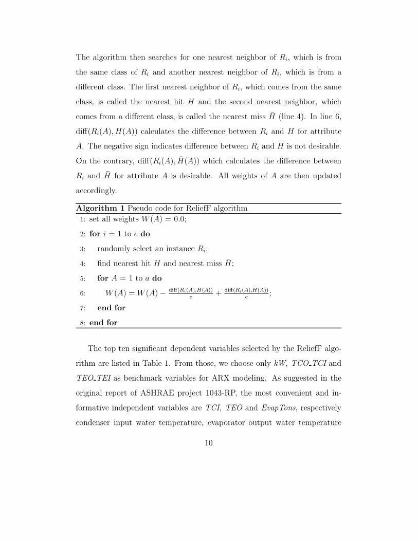
The algorithm then searches for one nearest neighbor of Ri, which is from
the same class of Ri and another nearest neighbor of Ri, which is from a
different class. The first nearest neighbor of Ri, which comes from the same
class, is called the nearest hit H and the second nearest neighbor, which
comes from a different class, is called the nearest miss H (line 4). In line 6,
diff(Ri(A), H(A)) calculates the difference between Ri and H for attribute
A. The negative sign indicates difference between Ri and H is not desirable.
On the contrary, diff(Ri(A), H(A)) which calculates the difference between
Ri and H for attribute A is desirable. All weights of A are then updated
accordingly.
Algorithm 1 Pseudo code for ReliefF algorithm
1: set all weights W (A) = 0.0;
2: for i = 1 to e do
3: randomly select an instance Ri;
4: find nearest hit H and nearest miss H;
5: for A = 1 to a do
6: W (A) = W (A)− diff(Ri(A),H(A))e
+ diff(Ri(A),H(A))e
;
7: end for
8: end for
The top ten significant dependent variables selected by the ReliefF algo-
rithm are listed in Table 1. From those, we choose only kW, TCO TCI and
TEO TEI as benchmark variables for ARX modeling. As suggested in the
original report of ASHRAE project 1043-RP, the most convenient and in-
formative independent variables are TCI, TEO and EvapTons, respectively
condenser input water temperature, evaporator output water temperature
10
Page 11
and tons of cooling delivered by the evaporator coil (a calculated variable).
Feature Description WeightkW Instantaneous input power 0.09402
TCO TCICondenser Water Temperature
Difference0.03724
TEO TEIEvaporator Water Temperature
Difference0.03545
PRE Evaporator Pressure 0.01854PRC Condensor Pressure 0.01699
TRC sub Subcooling 0.01512
kW/ton Chiller efficiency 0.01455
TEA Evaporator Approach Temperature 0.01378
TCA Condenser Approach Temperature 0.00859
Tsh dis Discharge Superheat 0.00026
Table 1: Ten most important features/variables selected from the original data set.
2.3. ARX Model
ARX models are a special type of the more general ARIMAX models.
ARIMAX models are, in theory, the most general class of dynamic models for
forecasting a non-stationary time series which can be stationarized (remove
drift in mean and variance) by transformations such as differencing. Con-
trary to regression models, the ARX representation fully characterizes the
dynamic nature of the process. Advantageously, the model parameters can
be estimated recuesively which is ideal for online implementation (e.g. [11]).
One possible limitation of the model is that it requires a time interval for the
estimation algorithm to recognize the impact of a fault on the parameters.
However, immediate detection of abnormal operations is not usually required
in HVAC plants. A reasonable delay (of the order of the largest time constant
11
Page 12
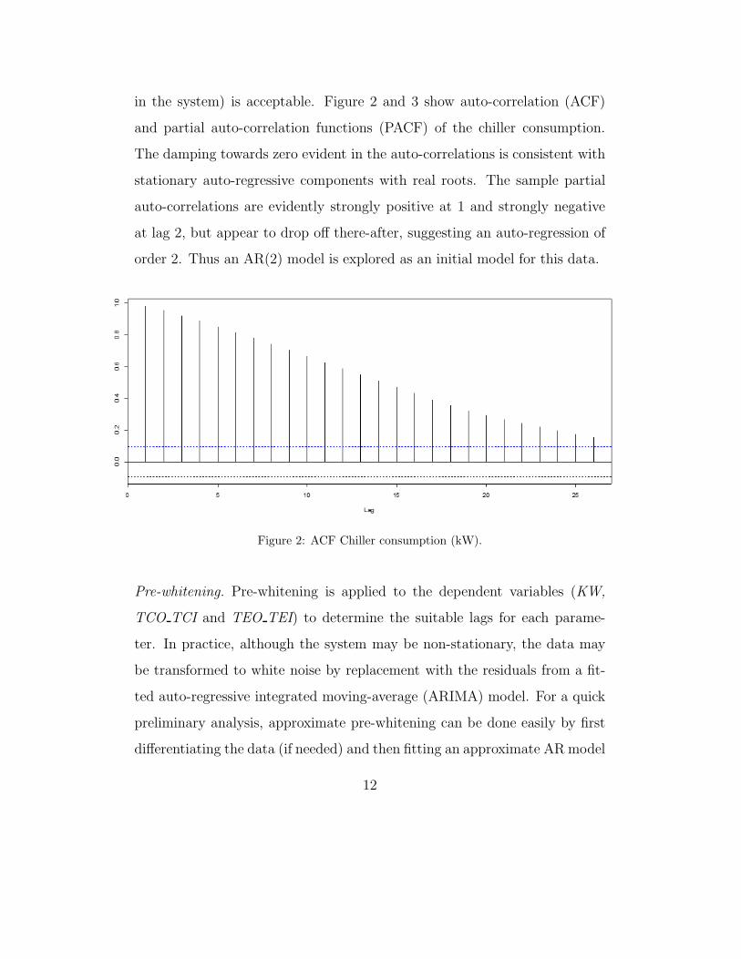
in the system) is acceptable. Figure 2 and 3 show auto-correlation (ACF)
and partial auto-correlation functions (PACF) of the chiller consumption.
The damping towards zero evident in the auto-correlations is consistent with
stationary auto-regressive components with real roots. The sample partial
auto-correlations are evidently strongly positive at 1 and strongly negative
at lag 2, but appear to drop off there-after, suggesting an auto-regression of
order 2. Thus an AR(2) model is explored as an initial model for this data.
Figure 2: ACF Chiller consumption (kW).
Pre-whitening. Pre-whitening is applied to the dependent variables (KW,
TCO TCI and TEO TEI) to determine the suitable lags for each parame-
ter. In practice, although the system may be non-stationary, the data may
be transformed to white noise by replacement with the residuals from a fit-
ted auto-regressive integrated moving-average (ARIMA) model. For a quick
preliminary analysis, approximate pre-whitening can be done easily by first
differentiating the data (if needed) and then fitting an approximate AR model
12
Page 13
Figure 3: PACF Chiller Consumption (KW).
with the order determined by minimizing the Akaike Information Criterion
(AIC) [25]. The pre-whitened data are then fitted to a model of the form
below,
Zt = β0 + β1Xt−i + ut, (1)
where Zt is a time series of the dependent variable, and Xt includes all
suitably lagged time series representations of the independent variables (ap-
propriately lagged values of TEO, TCI and EvapTons in this case) and ut
follows an ARIMA (p,d,q) model.
Lag Selection. The model defined by Equation 1 is known as the transfer-
function model. The specification of which lags of the independent variable
enter into the model is often done by inspecting the sample cross-correlation
function based on the pre-whitened data. When the model appears to require
13
Page 14
a fair number of lags of the independent variable, the regression coefficients
may be parsimoniously specified via an ARMA specification.
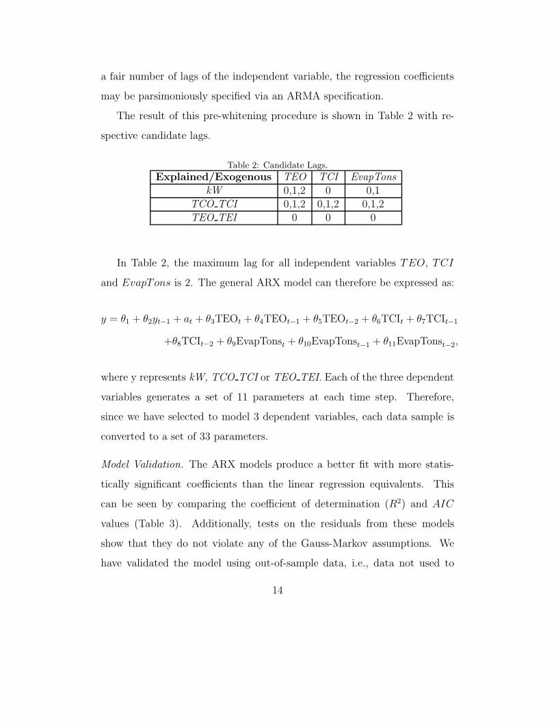
The result of this pre-whitening procedure is shown in Table 2 with re-
spective candidate lags.
Table 2: Candidate Lags.
Explained/Exogenous TEO TCI EvapTonskW 0,1,2 0 0,1
TCO TCI 0,1,2 0,1,2 0,1,2TEO TEI 0 0 0
In Table 2, the maximum lag for all independent variables TEO, TCI
and EvapTons is 2. The general ARX model can therefore be expressed as:
y = θ1 + θ2yt−1 + at + θ3TEOt + θ4TEOt−1 + θ5TEOt−2 + θ6TCIt + θ7TCIt−1
+θ8TCIt−2 + θ9EvapTonst + θ10EvapTonst−1 + θ11EvapTonst−2,
where y represents kW, TCO TCI or TEO TEI. Each of the three dependent
variables generates a set of 11 parameters at each time step. Therefore,
since we have selected to model 3 dependent variables, each data sample is
converted to a set of 33 parameters.
Model Validation. The ARX models produce a better fit with more statis-
tically significant coefficients than the linear regression equivalents. This
can be seen by comparing the coefficient of determination (R2) and AIC
values (Table 3). Additionally, tests on the residuals from these models
show that they do not violate any of the Gauss-Markov assumptions. We
have validated the model using out-of-sample data, i.e., data not used to
14
Page 15
estimated the parameters but corresponding to similar operating conditions.
The out-of-sample prediction, depicted in Figure 4, indicates that the ARX
model’s prediction performance is excellent with a Root-Mean-Square Devi-
ation (RMSE) of 1.98 (about 2.5% of the peak).
Table 3: R2 and AIC values comparison for using ARX model or linear regression equiv-alents
R2 AIC
ModelLinear
RegressionARX
LinearRegression
ARX
kW 0.9600 0.9850 2072.4992 1626.3739
TCO TCI0.9937 0.9989 -198.5449 -902.1029
TEO TEI 0.9999 0.9999 1866.426 1866.426
2.4. Support Vector Machine
In machine learning, the support vector machine is a supervised learning
model that categorizes data and recognizes patterns. For a given a set of
training data with known categories, an SVM machine is a model that assigns
to each data sample a point in a high dimensional space. In the next step,
the approach classifies the data by sub-dividing the high dimensional space
using hyper-planes. Ideally, the hyper-planes separate the training samples as
widely as possible to unambiguously distinguish new test sample categories.
The original SVM algorithm usually deals with two classes. An optimized
hyper-plane separates the training data set into two subsets by support vec-
tors [4]. In general, some key settings are required before the SVM starts: 1)
choosing kernel functions, such as polynomial, sigmoid, Gaussian radial basis
function (RBF), etc, and to map inputs onto a high dimensional space; 2)
15
Page 16
Time
valu
es
0 100 200 300 400
3040
5060
7080
Figure 4: Out-of-sample fit.
selecting SVM formulation, such as C-support vector classification (C-SVC),
v-support vector classification (v-SVC) and distribution estimation (one-class
SVM). These SVM formulations determine the classification algorithm used
to divide the sample space.
Suppose the training input consists of n samples, given a data sample
(x, c), where x ǫ X and c ǫ{+1,−1}, the classification function is expressed
in the dual space:
f(x) =
N∑
i=1
wiσi(x) + b. (2)
In this equation, σi is the kernel function predefined in the SVM model,
16
Page 17
and wi and b are the adjustable parameters of the classification function.
We choose the Gaussian radial basis function (RBF) as the kernel function
because of its superior performance in this application. The class z is decided
by the sign of f(x), or alternatively,
c =f(x)
‖f(x)‖. (3)
The basic SVM classifier only deal with two classes. For multi-class identi-
fication using SVM, we adopt the ‘one-against-all’ algorithm which constructs
one two-class SVM classifier between each pair of classes.
One-against-all Multi-class SVM. Consider an K−class classification prob-
lem, where we have N training samples: {x1, y1}, ..., {xN , yN}. Here xi ∈ Rm
is a m-dimensional feature vector and yi ∈ {1, 2, ..., K} is the corresponding
class label.
One-against-all approach constructs K binary SVM classifiers, each of
which separates one class from all the rest. The ith SVM is trained with
all the training examples of the ith class with positive labels, and all the
others with negative labels. Mathematically the ith SVM solves the following
problem that yields the ith decision function fi(x) = wTi φ(x) + bi:
Minimize:
L(w, εij) =1
2‖ wi ‖ +C
N∑
l=1
εij (4)
subject to yj(wTi ε(xj)) ≥ 1 − εij, ε
ij ≥ 0, where yj = 1 if yj = i and yj = −1
otherwise.
17
Page 18
At the classification phase, a sample x is classified as belonging to class:
ith = argmaxi=1,...,K
fi(x) = argmaxi=1,...,K
(wTi ε(x) + bi). (5)
2.5. An Overview of Proposed Hybrid Method
A hybrid approach combining ARX model and SVM is desirable to im-
prove the accuracy of the FDD analysis. In the proposed hybrid approach,
we pre-process the data using ARX models to remove auto- and cross-
correlations between variables. Then, we use parameters instead of the orig-
inal data to do the fault detection and diagnosis in SVM. The proposed
method includes seven separate steps:
(1) The original data set is divided into two parts. The first 2/3 is used as
historical data or training input. The rest 1/3 of the data are treated as
testing samples. The training data samples are categorized according
to their fault types (Normal, F1, F2,...,F5).
(2) Using ReliefF to select most important features, dependent and inde-
pendent variables are chosen, respectively. It is noted that each depen-
dent variable can be expressed as an equation of some or all independent
variables.
(3) The ARX model is trained by selected features. Each dependent vari-
able (kW, TCO TCI or TEO TEI) generates a set of 11 parameters at
each time step. Therefore, each data sample is converted to a set of
33 parameters. The whole original data set is transformed into a set of
ARX model parameters.
18
Page 19
(4) Two separate SVM are trained. The binary SVM library deals with
the fault detection and the multi-class SVM library diagnoses faults.
(5) The testing sample is pre-processed by the trained ARX model and
transformed into parameter set.
(6) The binary SVM library is applied to the testing parameter set to
detect faults. The positive result indicating normal operation data is
put aside waiting for final conclusion.
(7) If the result in step (7) is negative, the testing parameter set is input
into the multi-class SVM library. A deterministic fault type will be
assigned to that sample.
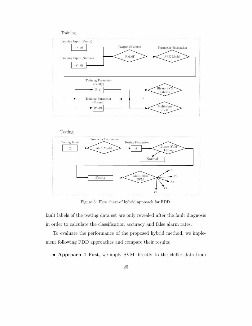
Finally, the prediction accuracy and false alarm rates can be concluded. The
overall flowchart is depicted in Figure 5.
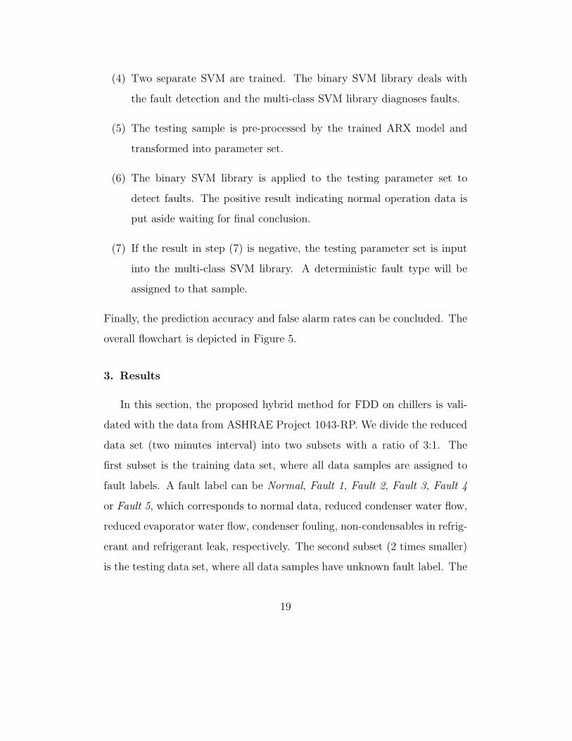
3. Results
In this section, the proposed hybrid method for FDD on chillers is vali-
dated with the data from ASHRAE Project 1043-RP. We divide the reduced
data set (two minutes interval) into two subsets with a ratio of 3:1. The
first subset is the training data set, where all data samples are assigned to
fault labels. A fault label can be Normal, Fault 1, Fault 2, Fault 3, Fault 4
or Fault 5, which corresponds to normal data, reduced condenser water flow,
reduced evaporator water flow, condenser fouling, non-condensables in refrig-
erant and refrigerant leak, respectively. The second subset (2 times smaller)
is the testing data set, where all data samples have unknown fault label. The
19
Page 20
Training Input (Normal)
(x∗, 0)
Training Input (Faulty)
(x, y)
ReliefF
Feature Selection
Training Parameter(Faulty)
(θ, y)
Training Parameter(Normal)
(θ∗, 0)
Binary SVMLibrary
Multi-classSVM
Training
Testing Input
x Binary SVMLibrary
Multi-classSVM
ARX Model
Parameter Estimation
ARX Model
Parameter EstimationTesting Parameter
θ
Normal
Faulty
F1
F2
F3
F5
Testing
F4
Figure 5: Flow chart of hybrid approach for FDD.
fault labels of the testing data set are only revealed after the fault diagnosis
in order to calculate the classification accuracy and false alarm rates.
To evaluate the performance of the proposed hybrid method, we imple-
ment following FDD approaches and compare their results:
• Approach 1 First, we apply SVM directly to the chiller data from
20
Page 21
ASHRAE Project 1043-RP.
• Approach 2 Second, we construct a static regression model similar
to the one suggested by the authors of the report of ASHRAE Project
1043-RP. The difference between the simulation results and the actual
data, i.e. the residuals of the regression model, are used for training
and testing in SVM.
• Approach 3 Third, we construct the ARX model and apply multilayer
perceptron neural network classifiers to the parameter set.
• Approach 4 Last, we construct the ARX model and apply SVM to
the parameter set.
Although the ARX model uses only the first three dependent variables
from Table 1, all 10 variables are used in Approach 1 and 2. Therefore, the
proposed hybrid model is severely handicapped in the comparison. Nonethe-
less, it manages to outperform other approaches as detailed below. To facili-
tate comparison, we separate the steps of fault detection and fault diagnosis.
Both the prediction accuracy and false alarm rates are reported.
3.1. Direct Application of SVM on Chiller Data
In this approach, we first train a binary SVM algorithm using the training
data and then perform the fault detection using the established model. The
detailed results are shown in Table 4. The prediction of level 1 faults is less
accurate than the others and the overall, because the data samples of level
1 faults are quite similar to normal operation. The SVM model failed to
21
Page 22
effectively distinguish the differences between them. The false alarm rates
are very high exceeding 10% in all cases.
Accu-racy(%)
Allfaults
F1 F2 F3 F4 F5FalseAlarm
All levels 72.09 67.03 96.93 87.02 98.66 77.67 20.22
level 1 69.47 62.37 88.55 76.48 94.66 55.73 12.98level 2 76.21 71.14 99.24 85.25 100.00 64.89 11.32
level 3 81.75 74.28 100.00 89.77 96.38 92.37 12.73level 4 85.19 88.20 100.00 89.82 100.00 97.71 13.44
Table 4: The fault detection accuracy and false alarm rates with different levels anddifferent types of faults resulting from the direct application of SVM on chiller data.
Accuracy(%)
Allfaults
F1 F2 F3 F4 F5
All levels 83.59 96.07 96.36 77.58 99.27 91.12
level 1 74.50 85.19 86.26 74.50 98.63 82.44level 2 85.50 99.24 99.39 76.69 99.39 86.41
level 3 89.11 99.54 99.54 82.36 99.37 96.63
level 4 89.77 99.54 99.54 84.12 99.54 98.17
Table 5: Results of fault diagnosis for direct application of SVM to chiller data.
The process of fault diagnosis is similar to that of fault detection except
that we use a multi-class SVM classifier to do the classification. In our work,
we use the ‘one against all’ algorithm based on SVM. The results are shown
in Table 5.
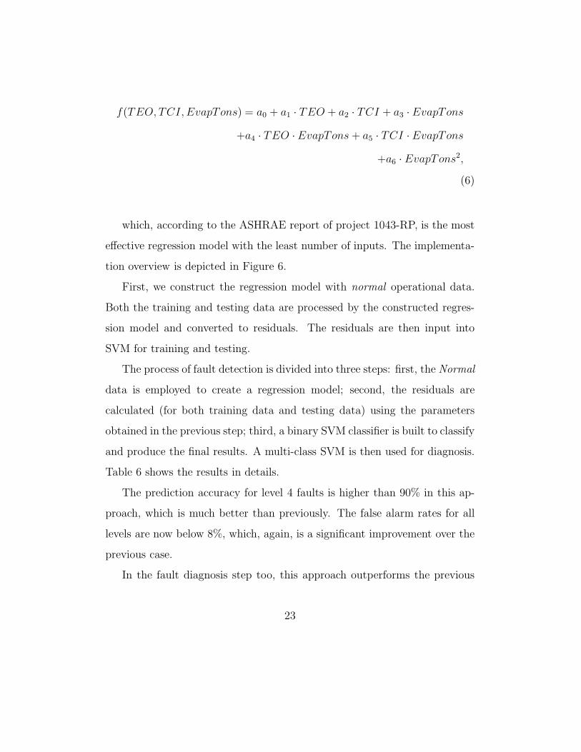
3.2. Application of SVM on Regression Model Residuals
The second procedure makes use of the regression model:
22
Page 23
f(TEO, TCI, EvapTons) = a0 + a1 · TEO + a2 · TCI + a3 ·EvapTons
+a4 · TEO ·EvapTons+ a5 · TCI ·EvapTons
+a6 · EvapTons2,
(6)
which, according to the ASHRAE report of project 1043-RP, is the most
effective regression model with the least number of inputs. The implementa-
tion overview is depicted in Figure 6.
First, we construct the regression model with normal operational data.
Both the training and testing data are processed by the constructed regres-
sion model and converted to residuals. The residuals are then input into
SVM for training and testing.
The process of fault detection is divided into three steps: first, the Normal
data is employed to create a regression model; second, the residuals are
calculated (for both training data and testing data) using the parameters
obtained in the previous step; third, a binary SVM classifier is built to classify
and produce the final results. A multi-class SVM is then used for diagnosis.
Table 6 shows the results in details.
The prediction accuracy for level 4 faults is higher than 90% in this ap-
proach, which is much better than previously. The false alarm rates for all
levels are now below 8%, which, again, is a significant improvement over the
previous case.
In the fault diagnosis step too, this approach outperforms the previous
23
Page 24
Training Residuals (Normal)
(∗, 0)
Binary SVM Library
Testing Residuals
¯
Normal
Training Residuals (Faulty)
(, y)
Faulty
Multi-Class SVM
Training
Training
F1 F2 F3 F5
Training Input (Normal)
(x∗, 0)
Testing Input
x
Training Input (Faulty)
(x, y)
Regression Model
Figure 6: Flow chart of the residual-based SVM approach.
approach in predicting all levels of faults.
3.3. Application of Neural Network to ARX Model Parameters
The third procedure constructs the ARX model and inputs parameters
into neural network classifiers to do the fault detection and diagnosis. We
compare the result of two neural networks: the radial basis function network
24
Page 25
Accu-racy(%)
Allfaults
F1 F2 F3 F4 F5FalseAlarm
All levels 82.58 78.04 99.81 92.84 100.00 89.23 7.38
level 1 72.39 68.46 99.24 81.02 100.00 80.19 6.23level 2 77.35 74.71 100.00 89.11 100.00 84.22 3.44
level 3 88.96 81.30 100.00 94.33 100.00 91.44 4.60
level 4 92.67 88.20 100.00 89.82 100.00 97.71 5.80
Table 6: The accuracy and false alarm rates of fault detection with different fault typesand levels after application of SVM on the regression model residuals
Accuracy(%)
Allfaults
F1 F2 F3 F4 F5
All levels 87.81 97.31 97.89 82.97 99.16 93.74level 1 75.42 90.38 92.67 79.08 98.47 84.89
level 2 88.55 99.54 99.39 86.11 99.24 93.13level 3 95.86 99.54 99.54 88.80 99.54 98.01
level 4 95.57 99.24 99.54 88.86 99.39 98.93
Table 7: Results of fault diagnosis combining SVM and regression model.
and multilayer perceptron network. The better result of the two, which is
obtained from the multilayer perceptron network, is shown in Table 8 and 9.
Accu-racy(%)
Allfaults
F1 F2 F3 F4 F5FalseAlarm
All levels 86.34 83.88 89.22 81.85 91.89 93.43 1.83
Level 1 82.33 79.22 80.09 77.34 88.72 89.48 3.58
Level 2 84.67 81.48 85.06 80.63 90.11 91.87 2.14
Level 3 90.26 92.27 93.88 84.87 93.07 95.72 0.90Level 4 94.44 93.45 99.82 89.76 95.07 97.93 0.05
Table 8: Results of fault detection combining multilayer perceptron network and ARXmodel.
25
Page 26
Accuracy(%)
Allfaults
F1 F2 F3 F4 F5
All levels 89.68 96.12 97.51 80.39 97.58 80.11
Level 1 82.34 95.33 93.86 77.80 95.96 76.34
Level 2 84.87 96.02 98.11 79.02 96.31 78.22
Level 3 92.85 98.87 99.83 88.27 98.98 86.19
Level 4 96.31 99.75 99.98 92.65 99.76 94.26
Table 9: Results of fault diagnosis combining multilayer perceptron network and ARXmodel.
3.4. Application of SVM to ARX Model Parameters
By applying SVM on the parameters generated by the ARX model, we
achieve the best overall result among all 4 procedures. Results are shown in
Table 10 and 11. Both prediction accuracy and false alarm rates are improved
significantly compared to the previous 3 approaches.
Accu-racy(%)
Allfaults
F1 F2 F3 F4 F5FalseAlarm
All levels 90.12 87.22 92.87 96.01 93.14 85.81 0.11
Level 1 79.63 74.76 81.13 81.39 74.19 79.33 0.49
Level 2 89.41 88.23 97.18 88.48 90.76 88.21 0.18
Level 3 96.32 98.65 93.57 98.73 95.24 91.71 0.00
Level 4 98.27 98.49 96.89 98.90 97.60 96.19 0.00
Table 10: Results of fault detection combining SVM and ARX model.
4. Conclusion
The primary contribution of this paper is that a robust FDD strategy
is proposed and developed to detect and diagnose chiller faults, based on a
26
Page 27
Accuracy(%)
Allfaults
F1 F2 F3 F4 F5
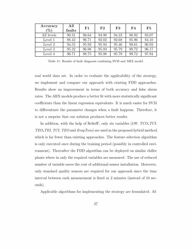
All levels 90.31 96.64 94.90 94.23 98.92 93.07
Level 1 88.42 96.71 92.02 92.68 95.96 84.10
Level 2 94.55 95.93 95.94 95.46 99.61 96.93
Level 3 95.32 96.98 95.93 95.79 99.72 96.17
Level 4 96.71 98.75 95.98 95.79 99.72 97.94
Table 11: Results of fault diagnosis combining SVM and ARX model.
real world data set. In order to evaluate the applicability of the strategy,
we implement and compare our approach with existing FDD approaches.
Results show an improvement in terms of both accuracy and false alarm
rates. The ARX models produce a better fit with more statistically significant
coefficients than the linear regression equivalents. It is much easier for SVM
to differentiate the parameter changes when a fault happens. Therefore, it
is not a surprise that our solution produces better results.
In addition, with the help of ReliefF, only six variables (kW, TCO TCI,
TEO TEI, TCI, TEO and EvapTons) are used in the proposed hybrid method,
which is far fewer than existing approaches. The feature selection algorithm
is only executed once during the training period (possibly in controlled envi-
ronment). Thereafter the FDD algorithm can be deployed on similar chiller
plants where in only the required variables are measured. The use of reduced
number of variable saves the cost of additional sensor installation. Moreover,
only standard quality sensors are required for our approach since the time
interval between each measurement is fixed at 2 minutes (instead of 10 sec-
onds).
Applicable algorithms for implementing the strategy are formulated. Af-
27
Page 28
ter training for generic chiller types, these algorithms can be integrated in
advanced building management systems to accurately detect and diagnose
the 5 faults commonly observed in chiller systems.
Future work will extend the application of the hybrid method to AHUs.
We are also finalizing a Kalman filter based estimation, which is suitable for
on-line parameter identification.
Acknowledgement
This research was supported by the Executive Affairs Authority (EAA) of
Abu Dhabi, United Arab Emirates as part of the project Predictive Mainte-
nance: Fault Detection and Diagnosis of AC Equipment. The authors would
also like to thank Mr Michael Vaughn and Ms Donna Daniel of ASHRAE
for their assistance in providing the chiller data of the ASHRAE Project
RP-1043.
Nomenclature
X training data set
N number of data samples
v a feature
Zt a time series of the dependent variable
Xt lagged time series representations of the independent variables
c type of class (binary)
28
Page 29
K number of classes (multi-class)
x a data sample in X
m number of features
y the class label
Y the set of class labels
x∗ a data sample in the training data set (normal operation)
x a data sample in the testing data set
ω the ARX model
θ parameters of the training data (faulty operation) processed by the ARX
model
θ∗ parameters of the training data (normal operation) processed by the ARX
model
θ parameters of the testing data processed by the ARX model
residuals of the training data (faulty operation) processed by linear regres-
sion model
∗ residuals of the training data (normal operation) processed by linear re-
gression model
¯ residuals of the testing data processed by linear regression model
29
Page 30
References
[1] P. R. Armstrong, C. R. Laughman, S. B. Leeb, and L. K. Norford. De-
tection of rooftop cooling unit faults based on electrical measurements.
International J. HVAC & R Research., 2006.
[2] M. C. Comstock and J. E. Braun. Experimental data from fault de-
tection and diagnostic studies on a centrifugal chiller. Ray W. Herrick
Laboratories, Purdue University, West Lafayette, IN, HL 99-18., 1999.
[3] M.C. Comstock, B. Chen, and J.E. Braun. Literature review for appli-
cation of fault detection and diagnostic methods to vapor compression
cooling equipment. Ray W. Herrick Laboratory Report HL 99-19., 1999.
[4] N. Cristianini and J. Shawe-Taylor. An introduction to support vector
machines and other kernel-based learning methods. Cambridge Univer-
sity Press, 2000.
[5] Z. Du, X. Jin, and X. Yang. A robot fault diagnostic tool for flow rate
sensors in air dampers and VAV terminals. Energy and Buildings 41
(3)., pages 279–286, 2009.
[6] J. Gertler. Fault detection and diagnosis in engineering systems. New
York: Marcel Dekker., 1998.
[7] H.T. Grimmelius, J.K. Woud, and G. Been. On-line failure diagnosis for
compression refrigerant plants. International Journal of Refrigeration
18(1)., pages 31–41, 1995.
30
Page 31
[8] H. Han, B. Gua, J. Kang, and Z.R. Li. Study on a hybrid SVM model
for chiller fdd applications. Applied Thermal Engineering, 2010.
[9] Y. Jia and T. Reddy. Characteristic physical parameter approach to
modeling chillers suitable for fault detection, diagnosis, and evaluation.
Journal of Solar Energy Engineering, Transactions of the ASME, v 125,
n 3, Emerging Trends in building Design, Diagnostics, and Operations,
pages 258–265, 2003.
[10] T. Kourti. Application of latent variable methods to process control and
multivariate statistical process control in industry. Journal of Adaptive
Control and Signal Processing., 2004.
[11] W. Y. Lee, Cheol Park, and George E. Kelly. Fault detection in an
air handling unit using residual and recursive parameter identification
method. ASHRAE Transactions 102(1)., 1996.
[12] S. Li. A model-based fault detection and diagnosis methodology for sec-
ondary HVAC system. Doctoral Dissertation, Drexel University., 2009.
[13] J. Liang and R. Du. Model-based fault detection and diagnosis of HVAC
systems using support vector machine method. International Journal of
Refrigeration., pages 1104–1114, 2007.
[14] Zhen Liu, Debao Ma, and Zhihong Feng. A feature selection algorithm
based on svm average distance. Measuring Technology and Mechatronics
Automation (ICMTMA), pages 90–93, 2010.
[15] Frederic Magoules, Hai-xiang Zhao, and David Elizondo. Development
31
Page 32
of an rdp neural network for building energy consumption fault detection
diagnosis. Energy and Buildings, 2013.
[16] G. Mustafaraja, J. Chen, and G Lowry. Development of room temper-
ature and relative humidity linear parametric models for an open office
using BMS data. Energy and Buildings, pages 348–356, 2010.
[17] N. Nassif, S. Moujaes, and M. Zaheeruddin. Self-tuning dynamic models
for HVAC system components. Energy and Buildings 40., pages 1709–
1720, 2008.
[18] M. H. Nguyen and Fernando de la Torre. Optimal feature selection for
support vector machines. Pattern Recognition, pages 584–591, 2010.
[19] H.C. Peitsman and V. Bakker. Application of black-box models to
HVAC systems for fault detection. ASHRAE Transactions 102(1).,
pages 628–640, 1996.
[20] M.A. Piette, S. Kinney, and P. Haves. Analysis of an information mon-
itoring and diagnostic system to improve building operations. Energy
and Buildings 33., pages 783–791, 2001.
[21] Bin Qi, Chunhui Zhao, Eunseog Youn, and Christian Nansen. Use
of weighting algorithms to improve traditional support vector machine
based classifications of reflectance data. Optics Express, Vol. 19, Issue
27, pages 26816–26826, 2011.
[22] J. Qin and S. Wang. A fault detection and diagnosis strategy of VAV
air-conditioning systems for improved energy and control performances.
Energy and Buildings 37 (10)., pages 1035–1048, 2005.
32
Page 33
[23] T.A. Reddy. Application of a generic evaluation methodology to assess
four different chiller fdd methods (rp-1275). HVAC and R Research, v
13, n 5., pages 711–729, 2007.
[24] Marko Robnik-Sikonja and Igor Kononenko. Theoretical and empirical
analysis of relieff and rrelieff. Machine learning, 53(1-2):23–69, 2003.
[25] Yosiyuki Sakamoto, Makio Ishiguro, and Genshiro Kitagawa. Akaike
information criterion statistics. Dordrecht, The Netherlands: D. Reidel,
1986.
[26] J. Schein, S. T. Bushby, N. S. Castro, and J. M. House. A rule-based
fault detectionmethod for air handling units. Energy and Buildings
38(12)., pages 1485–1492, 2006.
[27] Y.H. Song, Y. Akashi, and J.J. Yee. A development of easy-to-use tool
for fault detection and diagnosis in building air-conditioning systems.
Energy and Buildings 40 (2)., pages 71–82, 2008.
[28] B. G. C. C. Tuip, M. A. Houten, M. Trcka, and J. L. M. Hensen. Oc-
cupancy based fault detection on building level - a feasibility study.
Proceedings of the 10th International Conference Enhanced Building Op-
erations ICEBO, Kuwait, page 6, 2010.
[29] S. Wang and F. Xiao. AHU sensor fault diagnosis using principal com-
ponent analysis method. Energy and Buildings, 36(2)., pages 147–160,
2004.
[30] S. Wang, Q. Zhou, and F. Xiao. A system-level fault detection and
33
Page 34
diagnosis strategy for HVAC systems involving sensor faults. Energy
and Buildings 42 (4), pages 477–490, 2010.
[31] Yang Zhao, Shengwei Wang, and Fu Xiao. Pattern recognition-based
chillers fault detection method using support vector data description
(svdd). Applied Energy, 2013.
[32] Qiang Zhou, S. Wang, and F. Xiao. A novel strategy for the fault detec-
tion and diagnosis of centrifugal chiller systems. HVAC & R Research.,
2009.
34