arX

iv:a

stro

-ph/

9808

118v

1 1

2 A

ug 1

998

Stationary structures of irrotational binary systems – models for close binary

systems of compact stars

Koji Uryu1,2,3 and Yoshiharu Eriguchi 3

1International Center for Theoretical Physics, Strada Costiera 11, Trieste 34100, Italy2SISSA, Via Beirut 2-4, Trieste 34013, Italy

3Department of Earth Science and Astronomy, Graduate School of Arts and Sciences, University of Tokyo,

Komaba, Meguro, Tokyo 153, Japan

ABSTRACT

We propose a new numerical method to calculate irrotational binary systems composed of

compressible gaseous stars in Newtonian gravity. Assuming irrotationality, i.e. vanishing of

the vorticity vector everywhere in the star in the inertial frame, we can introduce the velocity

potential for the flow field. Using this velocity potential we can derive a set of basic equations for

stationary states which consist of (i) the generalized Bernoulli equation, (ii) the Poisson equation

for the Newtonian gravitational potential and (iii) the equation for the velocity potential with

the Neumann type boundary condition. We succeeded in developing a new code to compute

numerically exact solutions to these equations for the first time. Such irrotational configurations

of binary systems are appropriate models for realistic neutron star binaries composed of inviscid

gases, just prior to coalescence of two stars caused by emission of gravitational waves. Accuracies

of our numerical solutions are so high that we can compute reliable models for fully deformed

final stationary configurations and hence determine the inner most stable circular orbit of binary

neutron star systems under the approximations of weak gravity and inviscid limit.

Subject headings: binaries:close — black hole physics — hydrodynamics — instabilities —

methods: numerical — stars:black hole — stars:neutron — stars: rotation

1. Introduction

Historically, many authors have tried to obtain equilibrium configurations of self-gravitating close

binary systems. The classical attempts to solve this problem had been made by constructing approximate

solutions for binary systems. As is well known, the first quantitative approach was made by Roche who

treated a synchronously rotating incompressible fluid around a rigid sphere. By including appropriate

terms of the tidal potential from the sphere, the stationary state of the fluid can be approximated by an

ellipsoidal configuration. In order to treat more realistic situations, synchronously rotating incompressible

fluid-fluid binary systems were investigated by Darwin who also used the ellipsoidal approximation (see

e.g. Chandrasekhar 1969). For non-synchronously rotating binary systems, Aizenman (1968) studied

incompressible fluid binary systems with internal motion also by using the ellipsoidal approximation. The

situation has been changing for these 20 years. Not only incompressible binary systems but also compressible

binary configurations have been able to be constructed without using the ellipsoidal approximation, because

several powerful numerical schemes to obtain deformed self-gravitating stars have been developed (see e.g.

Eriguchi, Hachisu & Sugimoto 1982 ; Eriguchi & Hachisu 1983 ; Hachisu & Eriguchi 1984a ; Hachisu &

Eriguchi 1984b ; Hachisu 1986).

– 2 –

Apart from these developments for solving binary star systems, the problem of obtaining stationary

states of close binary star systems as exactly as possible has, recently, become one of the important issues

in relativistic astrophysics because they will provide models for binary neutron star systems just prior to

coalescence due to emission of gravitational waves (hereafter GW). Outcomes of such merging processes of

binary neutron star systems may be possible sources of astrophysically important phenomena such as γ-ray

bursts (see e.g. Paczynski 1986). Furthermore, coalescing binary systems are the promising sources of GW

which may be detected by the ground based interferometric detectors of GW in the early stage of the next

century (LIGO/VIRGO/TAMA/GEO, see e.g. Abramovici et al. 1992 ; Thorne 1994).

The evolution of such close binary neutron star systems due to GW emission can be approximated

well by quasi-stationary states until just before the coalescence stage, since the time scale in which the

binary separation decreases is longer than the orbital period (see e.g. Shapiro & Teukolsky 1983). The final

separation of two component stars where dynamical merging process starts is called an inner most stable

circular orbit (ISCO) of binary neutron stars (see Lai, Rasio & Shapiro 1993 and references therein). The

ISCO indicates implicitly the upper limit of the radius of neutron stars and hence gives some information

about the equation of state of the neutron matter. Consequently, in these several years, relativistic

astrophysicists have tried to solve equilibrium configurations of highly deformed close binary neutron star

systems by devising numerical schemes for the binaries. Theoretically obtained results for the ISCO is to be

compared with the observational data of GW detectors in the future, which will give important information

about the internal structure of neutron stars (Shibata 1997 ; Baumgarte et al. 1997a, 1997b, 1997c ; see

also Bonazzola, Gourgoulhon & Marck 1997 for a review).

The scenario of the final evolution of close binary neutron star systems was considered by

Kochanek (1992) and Bildsten & Cutler (1992). They pointed out that flow fields inside the component

stars of a binary system just prior to coalescence will be irrotational, i.e. the vorticity seen from the inertial

frame vanishes just prior to coalescence. According to their results, irrotationality is realized because the

viscosity of the neutron matter is too weak to synchronize the spin and the orbital angular velocity during

the evolution just before merging. It is precisely this stage of the binary evolution on which we will be

focussing in the present paper and, for this, the approximation of irrotationality seems likely to be very

good. We will explain the irrotational state in the next section.

In general, to construct stationary configurations of irrotational binary systems, it is necessary to treat

internal flows in the rotating frame of reference in which the stellar figure is seen to be fixed, although there

is fluid motion within the fixed figure. However, in most cases, it is very difficult to handle generic internal

flows or spins of stationary compressible stars not only for binary systems but also even for single stars.

Consequently, for compressible binary stars, numerical computations of fully deformed configurations have

been carried out only under the assumption that binary stars are rotating rigidly and synchronously or a

semi-analytic method by using the ellipsoidal approximation has been employed. In particular, Lai, Rasio

& Shapiro (1993b) developed the variational method in which the ellipsoidal approximation is used (LRS1

hereafter, see also Lombardi, Rasio & Shapiro 1997 for the post-Newtonian case). The exact treatment of

generic flows in such non-axisymmetric configurations has only been discussed by the present authors for

extended models of Dedekind-like configurations for compressible single stars (Uryu & Eriguchi 1996 and

the references therein).

However, for irrotational binary configurations, we recently succeeded in formulating a new scheme to

solve several types of new stationary states of irrotational binary systems in Newtonian gravity (Uryu &

Eriguchi 1998a, hereafter Paper I). We could develop that formulation by introducing the velocity potential

for the flow field. The new scheme is not only the first computation of binary configurations which are

– 3 –

rotating non-synchronously but also an important development to construct models for realistic neutron

stars in the inviscid limit. In this paper we will explain the computational scheme and discuss the results

in detail.

This paper is organized as follows. In section 2, we discuss the assumption of irrotationality, derive

the basic equations, and present boundary conditions. In section 3, we describe specific techniques used

in our actual numerical computations: choice of coordinate systems, introduction of the surface fitted

coordinate, non-dimensional variables and choice of physical parameters. The most delicate point in solving

the irrotational configurations is related to the way how to treat the elliptic partial differential equation

with the Neumann type boundary condition for the velocity potential. We introduce the solving method of

the velocity potential in detail in this section. We also explain the iteration procedure.

In section 4, computational results of our new scheme will be presented. In particular, we tabulate

the results for the irrotational gaseous star–gaseous star binary systems with equal mass. These solutions

correspond to so-called Irrotational Darwin-Riemann (IDR hereafter) configurations for compressible gases.

We also show the results for point source–irrotational gaseous star binary systems with various mass ratios.

These are so-called Irrotational Roche-Riemann (IRR hereafter) configurations for compressible stars. The

latter system can be considered to mimic configurations of black hole–neutron star systems. We compare

our results with those obtained under the ellipsoidal approximation by Lai, Rasio & Shapiro (hereafter LRS)

in a series of papers (Lai, Rasio & Shapiro 1993 (LRS1), 1994a hereafter LRS2, 1994b) and also with our

recent results for the irrotational solutions of incompressible binary systems which have been computed by

a totally different method from the present one (Uryu & Eriguchi 1998b, hereafter Paper II). Since the new

scheme turns out to be sufficiently accurate from this comparison, our solutions can be treated as reliable

ones even for highly deformed equilibrium configurations of compressible irrotational binary systems. By

using sequences of stationary solutions, the dynamical stability of binary systems can be discussed and the

final fate of binary neutron star systems can be clarified. This is related to the determination of the ISCO

for the binary systems as mentioned before. In section 5, we summarize our computational results and

discuss the remaining problems about the realistic close binary neutron star systems.

Our present results are not only extending the results of the classical problem of equilibrium

configurations of self-gravitating gases but also providing new realistic models of binary neutron star

systems such as a neutron star - neutron star system, or a black hole - neutron star system. In such

applications, we can regard the gaseous stars as models for neutron stars (NS) and the point sources as

models for black holes (BH).

2. Formulation for irrotational configurations

As discussed in Introduction, we will treat stationary states of inviscid and irrotational gaseous binary

star systems in this paper. Since the binary configurations are non-axisymmetric in nature, the system

cannot be stationary in the inertial frame. However, configurations can be in stationary states if seen from

a certain rotating frame whose angular velocity is that of the orbital motion of the binary star system.

First of all we will explain the validity of the irrotational assumption.

– 4 –

2.1. Validity of irrotationality for binary neutron star systems

As mentioned in Introduction, Kochanek (1992) pointed out that the velocity field of the component

inviscid star of a binary system just prior to coalescence becomes irrotational. This can be explained as

follows. For inviscid gases, Ertel’s theorem holds: the ratio of the vorticity vector in the inertial frame to

the density of a fluid element, ζ0/ρ, is conserved even under the existence of a potential force such as the

gravitational radiation reaction (Miller 1974). Here ρ is the density and the vorticity vector in the inertial

frame, ζ0, is defined as

ζ0(r) ≡ ∇× v(r) , (1)

where r and v(r) are the position vector of the fluid element and the velocity field seen from the inertial

frame, respectively. In the rotating frame in which the binary system can be seen in a quasi-stationary state

as mentioned above, the value of ζ0 can be regarded as negligibly small from the following reason. The

vorticity vector ζ0 can be expressed by using the vorticity vector in the rotating frame ζ and the orbital

angular velocity vector Ω as follows:

ζ0(r) = ζ(r) + 2Ω , (2)

where Ω is defined as Ω = Ω ez, ei (i = x, y, z) denotes the unit basis vector along the coordinate axis, z

is the direction parallel to the rotational axis of the orbital motion and Ω is the constant orbital angular

velocity. Here the vorticity vector ζ is also expressed by using the velocity vector of the fluid in the

rotational frame, u(r), by

ζ(r) ≡ ∇× u(r) . (3)

The above relation is derived by taking the curl of the following relation between the fluid velocity in the

inertial frame and that in the rotational frame,

v(r) = u(r) +Ω× r . (4)

Since the value of Ω at a close binary state is sufficiently larger than that of Ω and that of ζ at a

detached phase, and since ζ0 is conserved during evolution of a binary system, the contribution of ζ0 to the

final values of Ω and ζ can be totally negligible. Therefore we can consider that the realistic close binary

neutron star system originated from emission of GW is composed of irrotational gases, i.e.

ζ0(r) = 0 , (5)

everywhere.

Accordingly, for irrotational gases, we can assume the existence of the velocity potential, Φ(r), which

satisfies the following relation in the inertial frame:

v(r) ≡ ∇Φ(r) . (6)

2.2. Basic equations and boundary conditions

Since we will treat inviscid stars in Newtonian gravity, basic equations consist of the Euler equation,

the equation of continuity and the Poisson equation as follows:

∂ v

∂ t+ v · ∇v = −1

ρ∇p − ∇φ , (7)

– 5 –

∂ ρ

∂ t+ ∇ · (ρv) = 0 , (8)

φ = 4πGρ , (9)

where p, φ and G are the pressure, the gravitational potential and the gravitational constant, respectively.

For irrotational gases, the integrability condition for the equation (7) requires that the pressure must

be a function of the density, i.e. that the barotropic relation as follows must be satisfied:

p = p(ρ) . (10)

For barotropes, the Euler equation (7) can be integrated to the generalized Bernoulli equation. In the

rotating frame, the generalized Bernoulli equation is written as follows:

∂ Φ

∂ t− (Ω× r) · ∇Φ +

1

2| ∇Φ |2 +

∫

dp

ρ+ φ = f(t) , (11)

where f(t) is an arbitrary function of time. The origin of the position vector r for the fluid element in

the star is chosen at the point where the rotational axis intersects the equatorial plane. For simplicity, we

choose the following polytropic relation as the equation of state:

p = Kρ1+1/N = KΘN+1 , (12)

where Θ, N and K are the Emden function which is proportional to the enthalpy, the polytropic index and

a certain constant, respectively. Note that the Emden function defined here is different in normalization

from that usually employed in spherical polytropic stars. The equation of continuity (8) is also rewritten

by using the velocity potential Φ as follows:

∂ ρ

∂ t+ ∇ · (ρ∇Φ) = 0 . (13)

Since we assume stationarity of configurations in the rotating frame, we can set following conditions:

∂ ρ

∂ t≡ 0

∂ Φ

∂ t≡ 0 and f(t) = C = constant . (14)

Therefore, we can rewrite equations (11) and (13) as follows:

Θ =1

K (N + 1)

[

(Ω× r) · ∇Φ − 1

2| ∇Φ |2 − φ + C

]

, (15)

and

Φ = N(Ω× r − ∇Φ) · ∇Θ

Θ, (16)

where we use the relation (12).

As for the Poisson equation (9), we use the integral form as follows:

φ(r) = −G

∫

V

ρ(r′

)

| r− r′ |d

3r′

, (17)

where the integration is performed over the whole volume of the stars V . The boundary condition for φ is

automatically included in this expression. For point source models, the gravitational potential of the point

source (BH) is expressed as

φBH (r) = − GMBH

| r− rBH | , (18)

– 6 –

where MBH and rBH are the mass and the position vector of the point source, respectively. If we substitute

these expressions for the gravitational potentials into the equation (15), we obtain two equations for two

field variables, the Emden function Θ(r) and the velocity potential Φ(r).

Boundary conditions for these two variables are as follows. The pressure and accordingly the Emden

function should vanish on the stellar surface because of the definition of the surface itself. Concerning

the velocity potential, the fluid element on the stellar surface should flow along it in the rotational frame

because of stationarity of the configuration. Geometrically speaking, it means that the fluid velocity on

the surface in this frame uS is perpendicular to the normal of the stellar surface nS , where the subscript S

denotes the stellar surface. Thus these boundary conditions are written as follows:

Θ(rS) = 0 , (19)

nS · uS = nS · (∇Φ − Ω× rS) = 0 , (20)

where we use the relation (4) and we denote the position vectors of points on the stellar surface by rS . The

former condition determines the shape of stellar surface. As seen from the form of the equation of continuity

(16) and from that of the boundary condition (20), the problem is reduced to an elliptic partial differential

equation with a Neumann type boundary condition. From the standpoint of numerical computations,

careful treatment is required to solve this kind of equations. Thus we will explain the solving scheme of

that equation to some extent.

2.3. Integral form of the Neumann problem

Here we consider the following Neumann problem:

Φ = S(r) , (21)

nS · ∇Φ|S = nS · (Ω× rS) , (22)

where S(r) is defined as

S(r) = N(Ω× r − ∇Φ) · ∇Θ

Θ. (23)

As is well known, a solution of the Neumann problem for the elliptical partial differential equation (21)

can be expressed as follows:

Φ(r) = − 1

4π

∫

V

S(r′)

| r− r′ |d

3r′

+ χ(r) , (24)

where χ(r) is a regular homogeneous solution to the Laplace equation inside the star, i.e.

χ(r) = 0 . (25)

Note that the integral is performed on V which is a volume of one gaseous component star. Substituting

the above expression to the l.h.s. of the boundary condition (22), we have the following equation:

− 1

4π

∫

V

nS ·(

∇ 1

| r− r′ |

)

S

S(r′)d3r′

+ nS · ∇χ(r)|S = nS · (Ω× rS) . (26)

It should be noted that this is a formal solution because there appears the unknown function Φ in the

source term. In other words, this is an integral equation for unknowns. Thus, once the Emden function is

given, the velocity potential can be obtained by solving equations (24), (25) and (26).

– 7 –

3. Implementation for actual computations

In the previous section, we have written down the basic equations for the irrotational binary

configurations. For our actual computations, we use equations (15), (24) and (25) and the boundary

conditions (19) and (26). We will find solutions to these equations by using an iterative scheme explained

later. To accomplish a robust iteration scheme to converged solutions, we need to devise several techniques

which have been obtained after a number of attempts to solve equilibrium configurations of rotating stars.

We will describe some techniques in this section: choice of the coordinates, choice of parameters and the

iteration scheme. Since the Neumann problems have not been treated in the theory of rotating stars except

for Eriguchi (1990), we will explain the solving method for it in detail.

3.1. Choice of coordinates

Since we treat the BH–NS binary systems or the equal mass NS–NS binary systems, we only need

to compute structures of one gaseous component star. The Cartesian coordinates (x, y, z) whose origin is

located at the intersection of the rotational axis and the equatorial plane are used where the rotational axis

coincides with the z-axis and the equatorial plane is the x-y plane. We assume that the configuration of

a component star is symmetric about the x-y and x-z planes. The distribution of the velocity potential

is symmetric about the x-y plane but anti-symmetric about the x-z plane. The centers of the stars are,

therefore, on the x-axis. For the equal mass IDR (NS–NS) binary systems, we also assume symmetry about

the y-z plane for the density and anti-symmetry about the y-z plane for the velocity potential. In actual

computations, we introduce a spherical coordinate system (r, θ, ϕ) whose origin is fixed at the geometrical

center of the gaseous component star (NS) on the x-axis with a distance from the rotational axis dNS as

follows:

dNS ≡ Rout + Rin

2, (27)

where Rout and Rin are distances from the rotational axis to the inner and outer edges of the star on the

x-axis, respectively. The angle θ is the zenithal angle measured from the positive direction parallel to the

z-axis and the angle ϕ is the azimuthal angle measured from the positive direction of the x-axis. Relations

between the Cartesian coordinates and the spherical coordinate systems are expressed as follows:

x = dNS + r sin θ cosϕ ,

y = dNS + r sin θ sinϕ , (28)

z = r cos θ .

Since deformation of the stellar surface from a sphere is not so large for binary stars, we may consider the

stellar surface as a single-valued function of θ and ϕ and write it as R(θ, ϕ) in this coordinate. Since we

need to solve the equation with the boundary condition (26) on the surface, the function R(θ, ϕ) plays an

important role in our numerical method.

In this spherical coordinate system (28), we can expand the Green’s function of the gravitational

potential and the velocity potential, 1/ | r− r′ |, by using the Legendre polynomials. For the contribution

from its own component, it is expanded as

1

| r− r′ | =

∞∑

n=0

fn(r, r′)Pn(cosβ(θ, ϕ; θ

′ϕ′)) , (29)

– 8 –

where fn(r, r′) is defined as,

fn(r, r′) =

1

r

(

r′

r

)n

for r′ ≤ r ,

1

r′

( r

r′

)n

for r ≤ r′ .

(30)

Here Pn is the Legendre function and cosβ(θ, ϕ; θ′ϕ′) is defined as

cosβ(θ, ϕ; θ′ϕ′) = cos θ cos θ′ + sin θ sin θ′ cos(ϕ− ϕ′) . (31)

Concerning the gravitational potential for the IDR systems, the contribution from the other component

becomes as follows:1

| r− r′ | =

∞∑

n=0

r′n

Dn+1Pn(cos γ(θ, ϕ; θ

′ϕ′)) , (32)

where D and cos γ are defined as

D =

(2dNS )2 + r2 + 2dNS r sin θ cosϕ

1/2, (33)

and

cos γ(θ, ϕ; θ′ϕ′) =2 dNS sin θ′ cosϕ′ + r cosβ(θ, ϕ; θ′ϕ′)

D, (34)

respectively. In this case the dashed variables should be considered to belong to the other component star.

Finally, several terms in the basic equations are written explicitly in this coordinates as follows:

| ∇Φ |2 =

(

∂ Φ

∂ r

)2

+

(

1

r

∂ Φ

∂ θ

)2

+

(

1

r sin θ

∂ Φ

∂ ϕ

)2

, (35)

(Ω× r) · ∇Φ = Ω∂ Φ

∂ ϕ+ Ω dNS

(

sin θ sinϕ∂ Φ

∂ r+

cos θ sinϕ

r

∂ Φ

∂ θ+

cosϕ

r sin θ

∂ Φ

∂ ϕ

)

. (36)

3.2. Surface fitted coordinate

In our actual computations, we transform the basic equations into the surface fitted spherical

coordinates (see e.g. Eriguchi & Muller 1985 ; Uryu & Eriguchi 1996). New coordinates (r∗, θ∗, ϕ∗) are

defined by

r∗ =r

R(θ, ϕ), θ∗ = θ , and ϕ∗ = ϕ . (37)

By this transformation, the stellar interior is mapped into a computational domain given by

r∗ ∈ [0, 1] , θ∗ ∈ [0, π] , and ϕ∗ ∈ [0, 2π] . (38)

Accordingly, the derivatives are transformed as follows:

∂

∂ r−→ D∗

r =1

R

∂

∂ r∗, (39a)

∂

∂ θ−→ D∗

θ =∂

∂ θ∗− r∗

R

∂R

∂ θ∗D∗

r , (39b)

∂

∂ ϕ−→ D∗

ϕ =∂

∂ ϕ∗− r∗

R

∂R

∂ ϕ∗D∗

r . (39c)

– 9 –

Since transformation of the equations into this surface fitted coordinates (37) is straightforward, we do not

explicitly write them down in this paper.

The disadvantage of utilizing this surface fitted coordinate is that we cannot decrease the number

of floating calculations which appear in the integral equations (17) and (24) by arranging the order of

computations. So it requires a large amount of CPU time and hence we cannot treat a large number of grid

points for numerical computations. On the other hand, the advantage of this coordinate is that it is easy

to treat the derivatives on the surface and also the surface itself. Consequently, it improves the robustness

and accuracy of the computational scheme. Furthermore, we do not need to treat vacuum regions. Thus

this advantage cancels out the disadvantage of a small number of mesh points.

3.3. Non-dimensional variables and choice of parameters

The choice of the parameters in computing the equilibrium configurations is crucial to construct a

robust numerical method. In our actual computations, we use non-dimensional variables as follows:

r =r

R0, ∇ = R0 ∇ , = R2

0 , ρ =ρ

ρc, Θ =

Θ

ρ1/Nc

,

p =p

pc, v =

v√Gρc R0

, Φ =Φ√

Gρc R20

, Ω =Ω√Gρc

, (40)

φ =φ

GρcR20

, C =C

GρcR20

, β =pc

Gρ2R20

, alm =alm

Rl−20

,

where R0 is the geometrical radius of the gaseous component star (NS) along the x axis, that is

R0 = (Rout −Rin)/2, ρc and pc are the density and the pressure at the coordinate center r = 0 of the star.

Furthermore, an unknown quantity β, which is related to a scale of distance, appears in the Bernoulli’s

equation (15) as follows:

Θ =β

N + 1

[

(Ω× r) · ∇ Φ − 1

2| ∇ Φ |2 − φ + C

]

. (41)

For equal mass IDR (NS–NS) binary systems, in order to solve one stationary model, we need to

specify or determine the following four quantities in addition to the two quantities Θ and Φ:

dNS , Ω, β and C . (42)

Of these quantities, we can specify the value of dNS arbitrary. The other three quantities can be obtained

by employing the following conditions:

R(π/2, 0) = 1 , R(π/2, π) = 1 , and Θ(0, θ, ϕ) = 1.0 . (43)

From these conditions, we can solve for the three quantities as follows:

Ω =

12

[

(

∂ Φ∂ϕ

)2

out−(

∂ Φ∂ϕ

)2

in

]

+ φout − φin

(1 + dNS )(

∂ Φ∂ϕ

)

out− (1− dNS )

(

∂ Φ∂ϕ

)

in

, (44)

C = − Ω(1 + dNS )

(

∂ Φ

∂ϕ

)

out

+1

2

(

∂ Φ

∂ϕ

)2

out

+ φout , (45)

– 10 –

β =N + 1

[

(Ω× r) · ∇Φ − 12 | ∇Φ |2 − φ + C

]

c

, (46)

where subscripts out, in and c mean the quantities at the outer edge, at the inner edge and at the

geometrical center of the star, respectively.

For IRR (BH–NS) binary systems, since we will treat non-equal mass configurations, in order to get

one stationary model, we need to specify or determine the following six quantities in addition to the two

quantities Θ and Φ:

dNS , dBH , Ω, β, C, and MBH , (47)

where two distances from the rotational axis to each component star are expressed as dNS and dBH . These

distances appear in the gravitational potential of the point source, i.e. equation (18),

φBH = −GMBH

DBH

, (48)

where

DBH =

(dBH + dNS )2 + r2 + 2(dBH + dNS ) r sin θ cosϕ

1/2. (49)

Among these six parameters, two quantities can be freely specified: the separation between a point

source and a gaseous star, dNS + dBH , and the mass ratio of two components, MNS/MBH . Three quantities

Ω, C and β can be determined from the same equations above. Since the motion of the point mass which

is subject to the gravitational force of the gaseous component star should be Keplerian, we can impose the

following relation:

dBH Ω2 =

∞∑

n=0

In

(dNS + dBH )n+2, (50)

where In is defined as follows,

In = (n+ 1)

∫ 1

0

r′2dr′

∫ π

0

sin θ dθ

∫ 2π

0

dϕ r′n ρ(r′, θ′, ϕ′)Pn(cos γ(π/2, π; θ

′, ϕ′)) . (51)

These equations (44), (45) and (46), and (50) for the IRR systems are simultaneously solved in the

computational scheme.

3.4. Discretization and iteration procedure

We discretize our basic equations, which are composed of the differential-integral equations, on the

equidistantly spaced grid points in the surface fitted coordinates. The derivatives are approximated by using

the ordinary central difference scheme of the second order and the integrations are performed by employing

the trapezoidal formula. Let us denote discrete mesh points as (r∗i , θ∗j , ϕ

∗

k) where 0 ≤ i ≤ Nr , 0 ≤ j ≤ Nθ

and 0 ≤ k ≤ Nϕ and Nr, Nθ and Nϕ are certain numbers employed in the approximation. In our actual

computations, we have used the following number of grid points: (Nr, Nθ, Nϕ) = (16, 8, 16). The number of

terms used in the Legendre expansion which appears in equations (29), (32) and (51) is taken into account

up to Nl = 10 instead of infinity.

We apply the iteration scheme to these discretized equations. It is basically identical to the

self-consistent-field (SCF hereafter) method developed by Ostriker and Mark (1968) and extended so as to

– 11 –

compute various equilibrium configurations of self-gravitating stars by Hachisu (Hachisu 1986 ; Komatsu,

Eriguchi & Hachisu 1989). Although there is no rigorous proof for the convergence to a solution and its

convergence becomes slower for some complicated systems (e.g. Yoshida & Eriguchi 1997), the SCF scheme

has been proved very powerful for solving structures of rapidly rotating stars as far as proper choice of

model parameters is made. Here we have succeeded in finding proper parameters and have been able to

construct a computational code which works well for our present problem. It should be noted that the

memory and the CPU time required for the SCF scheme are relatively small, although we need to use not a

small amount of the memory and the CPU time to get accurate 3D configurations.

We will briefly explain our iteration scheme. As seen from our basic equations (15) and (24), we can

symbolically express the discretized versions of these basic equations as follows. Let us denote the basic

variables Θ and Φ by Qi where subscript i means the discretized value of the quantity Q at the i-th mesh

point. The discretized basic equations are written as

Qj = Fj [Qi] , (52)

where Fj means the non-linear functional of variables. These equations must be organized consistently. In

other words, the total number of Qi needs to be the same as that of Fj .

In our iteration scheme or, in general, in the SCF scheme, this equation is used as follows:

Q(new)j = Fj [Q

(old)i ] . (53)

Therefore, if we have some initial guesses for physical quantities, we will be able to obtain new values for

the quantities by substituting the approximate values of physical quantities into the r.h.s of equation (53).

Hopefully newly obtained values for variables on l.h.s. can be improved ones.

Our actual iteration procedure of the scheme is organized as follows:

(i) preparation of initial guesses for Θ and Φ,

(ii) computation of values for ρ and φ and gradients of Φ given in step(i),

(iii) computation of new values for Θ by using equation (15),

(iv) computation of new values for R by using values of Θ,

(v) computation of values for ρ and φ and gradients of Φ and Θ,

(vi) computation of new values for Φ by using equation (24),

(vii) computation of gradients of Φ again,

(viii) computation of new values for parameters,

(ix) checking of convergence of all quantities; if not, go back to step (iii).

As mentioned before, although there are no rigorous mathematical theorems for convergence of the SCF

method, we have succeeded in constructing a scheme which accomplishes a convergence by using the above

procedure. We have used a certain parameter for improvement as follows:

Q(new)j = b Fj [Q

(old)i ] + (1 − b)Q

(old)j , (54)

– 12 –

where the first term of r.h.s. is the improved quantities and b is a numerical factor which is introduced to

avoid jumping of solutions to very different values and to make the iteration converge. Thus we will call

this a convergence factor. We have set b = 1/4 ∼ 1 and used relatively smaller values for polytropes with

larger N . Typically we obtain converged solutions after 20 ∼ 50 iterations for IDR models or IRR models

with nearly equal masses. For IRR models with larger mass ratio, 40 ∼ 80 iterations were needed. The

CPU time was approximately 5.2 minutes per 1 iteration for IDR binary systems and 2.9 minutes per 1

iteration for IRR binary systems by using the Fujitsu VX/1R vector computer.

3.5. Solving method for the homogeneous term of the velocity potential

Finally we present the solving method for the homogeneous term of the velocity potential. Since the

first term alone in equation (24) does not satisfy the boundary condition on the surface, we need to add

the second term, χ(r), i.e. the homogeneous solution of the Laplace equation. In the spherical coordinates,

homogeneous solutions to equation (25) can be expressed by using the spherical harmonic functions as

follows:

χ(r, θ, ϕ) =

∞∑

l=1

l∑

m=1

alm rl[

1 + (−1)l+m]

Y ml (cos θ) sin mϕ , (55)

where alm’s are certain constants and Y ml (cos θ) are the spherical harmonic functions. Here we have

taken into account that solutions must be regular at the center and that the velocity potential is assumed

symmetric about the x-y plane and anti-symmetric about the x-z plane.

These coefficients alm are determined from the boundary condition (26) on the stellar surface. After

substituting the above expression (55) into equation (26), we can obtain the coefficients alm by applying the

least square method to the discretized version of the boundary condition (26). To explain the procedure,

we symbolically write the discretized boundary condition as follows:

Nl∑

l=1

l∑

m=1

almF ml (θi, ϕj) − H(θi, ϕj) = 0 , (56)

where F ml and H are certain functions. To apply the least square method, we sum up the square of the

l.h.s of the above equation at all grid points on the surface and obtain the following equation:

E =∑

i,j

[

Nl∑

l=1

l∑

m=1

almF ml (θi, ϕj) − H(θi, ϕj)

]2

= 0 . (57)

Coefficients alm can be solved by finding solutions to the equations which are derived by minimizing the

value of E as follows:δ Eδ alm

= 0 . (58)

Here we will explicitly write down some terms in equation (26). We need a gradient orthogonal to the

stellar surface R(θ, ϕ). It is written as

nS · ∇g|S =1√h

(

∂ g

∂ r− 1

R2

∂ R

∂ θ

∂ g

∂ θ− 1

R2 sin2 θ

∂ R

∂ ϕ

∂ g

∂ ϕ

)

S

, (59)

where g is a certain function and h is defined as

h(θ, ϕ) = 1 +

(

1

R

∂ R

∂ θ

)2

+

(

1

R sin θ

∂ R

∂ ϕ

)2

. (60)

– 13 –

The term nS · (Ω× rS) is expressed as

nS · (Ω× rS) =1√h

−Ω∂ R

∂ ϕ+ Ω dNS

(

sin θ sinϕ − cos θ sinϕ

R

∂ R

∂ θ− cosϕ

R sin θ

∂ R

∂ ϕ

)

. (61)

4. Sequences of irrotational binary

Our new formulation for irrotational binary configurations explained in the previous sections has worked

nicely so that we can obtain stationary sequences of binary stars for many different model parameters.

Since we assume polytropic stars in Newtonian gravity, one stationary model of a binary system which

consists of completely identical stars can be specified only by two parameters: the polytropic index N and

the separation of two stars. Thus for compressible IDR binary systems, one stationary sequence is defined

as a sequence with a fixed value for the polytropic index N but with changing the value of the separation.

On the other hand, for compressible IRR binary systems, we have one more parameter to characterize a

sequence, which is the mass ratio MNS/MBH of a gaseous star (NS) to a point source (BH).

A sequence with fixed masses for component stars and with the prescribed equation of state can

be regarded as an evolutionary sequence due to emission of GW since the irrotationality assures the

conservation of circulation as discussed in section 2.1 (Miller 1974; Eriguchi, Futamase & Hachisu 1990).

Concerning this evolutionary or stationary sequence, LRS1 showed that dynamical instability will set in

at the point on the sequence where the total angular momentum J(dG) or the total energy E(dG) of the

binary system attains its local minimum. Here dG is the separation of two centers of mass of component

stars. They also proved that the distance at the minimum point for J(dG) and that for E(dG) coincide for

a stationary sequence. This property of a sequence can also be applied for the present results. We will call

this point the dynamical instability limit and denote the corresponding separation by rd. This dynamical

instability limit may or may not be reached before the point of termination of the sequence of equilibrium

models. The minimum separation for equilibrium configuration is referred to as the Roche limit rR. For the

equal mass IDR binary systems, there is another type of critical point which is the contact limit where the

two gaseous components come to touch each other at the inner edges. We denote this contact separation

by rc. We will refer to these characteristic separations as the critical separations.

It is important to know behaviors of J(dG) and/or E(dG) along stationary sequences because final

states of evolution will be affected by the relation among those critical separations. Since GW carry away

the angular momentum as well as the energy, the separation of a binary system will decrease as the system

evolves. If rd is larger than two other critical separations, i.e. rR and rc, two component stars will begin to

merge on a dynamical time scale because of the orbital instability. On the other hand, if rd is smaller than

the other critical separations, other hydrodynamical phenomena is expected to occur. In particular, for

the IDR binary systems, the contact dumbbell configurations may appear similarly to the incompressible

case (Eriguchi & Hachisu 1985) and for the IRR binary systems the Roche lobe overflow may occur. We

will discuss this matter later by comparing our results with those of recent hydrodynamical simulations of

binary systems by several authors.

In the following subsections, we will tabulate physical quantities which characterize the sequences.

In Tables we show the following quantities. They are the normalized values for the separation of the

geometrical centers of two component stars, i.e. d = 2dNS for the IDR systems, and d = dBH + dNS for the

IRR systems, the separation of mass centers of two component stars dG, the angular velocity Ω, the total

– 14 –

angular momentum J and total energy E. These quantities are normalized as follows:

dG =dGRN

for IDR , dG =dGRN

(

MNS

MBH

)1

3

for IRR ,

Ω =Ω

(πGρN )1/2, J =

J

(GM3RN )1/2and E =

T + W + U

GM2/RN, (62)

where M is the mass of primary star, RN is the radius of the spherical polytrope with the same mass

M and with the same polytropic index N . The quantity ρN is defined as ρN = M/(4πR3N/3). These

normalizations are the same as those adopted in LRS’s papers.

The quantities T , W and U are the total kinetic energy, the total potential energy and the total

thermal energy defined as usual (see e.g. Tassoul 1978). The separation between the mass centers of two

component stars dG is computed as follows:

dG = 2

∫

V x ρ d3r′

Mfor IDR, dG =

∫

V x ρ d3r′

M+ dBH for IRR. (63)

The total angular momentum J is computed by using the velocity potential as follows:

J = 2

∫

V

ρ (r× v) · ezd3r′

= 2

∫

V

ρ

∂ Φ

∂ ϕ+ dNS

(

sin θ sinϕ∂ Φ

∂ r+

cos θ sinϕ

r

∂ Φ

∂ θ+

cosϕ

r sin θ

∂ Φ

∂ ϕ

)

d3r′

for IDR, (64)

J =

∫

V

ρ (r× v) · ezd3r′

+ MBH d2BH Ω for IRR. (65)

The quantity T/ |W | is also tabulated but note that the definition is different from LRS1. The value of the

virial constant VC normalized by the total gravitational potential is computed as follows:

VC =| 2T + W + 3U/N |

|W | , (66)

where the value of U/N vanishes for the models with N = 0. We also show the values of R which

corresponds to average radius defined as follows:

R =

(

3V

4 π R3N

)1

3

=

[

1

4 π R3N

∫ π

0

sin θ dθ

∫ 2π

0

dϕR3(θ, ϕ)

]

1

3

. (67)

Generally, this quantity increases as the separation decreases. It indicates that the volume of the gaseous

star always increases and, accordingly, the central density decreases as the two component star approaches

during the evolution.

4.1. Compressible IDR binary systems with equal mass

4.1.1. Accuracy of the new numerical method and stationary sequences

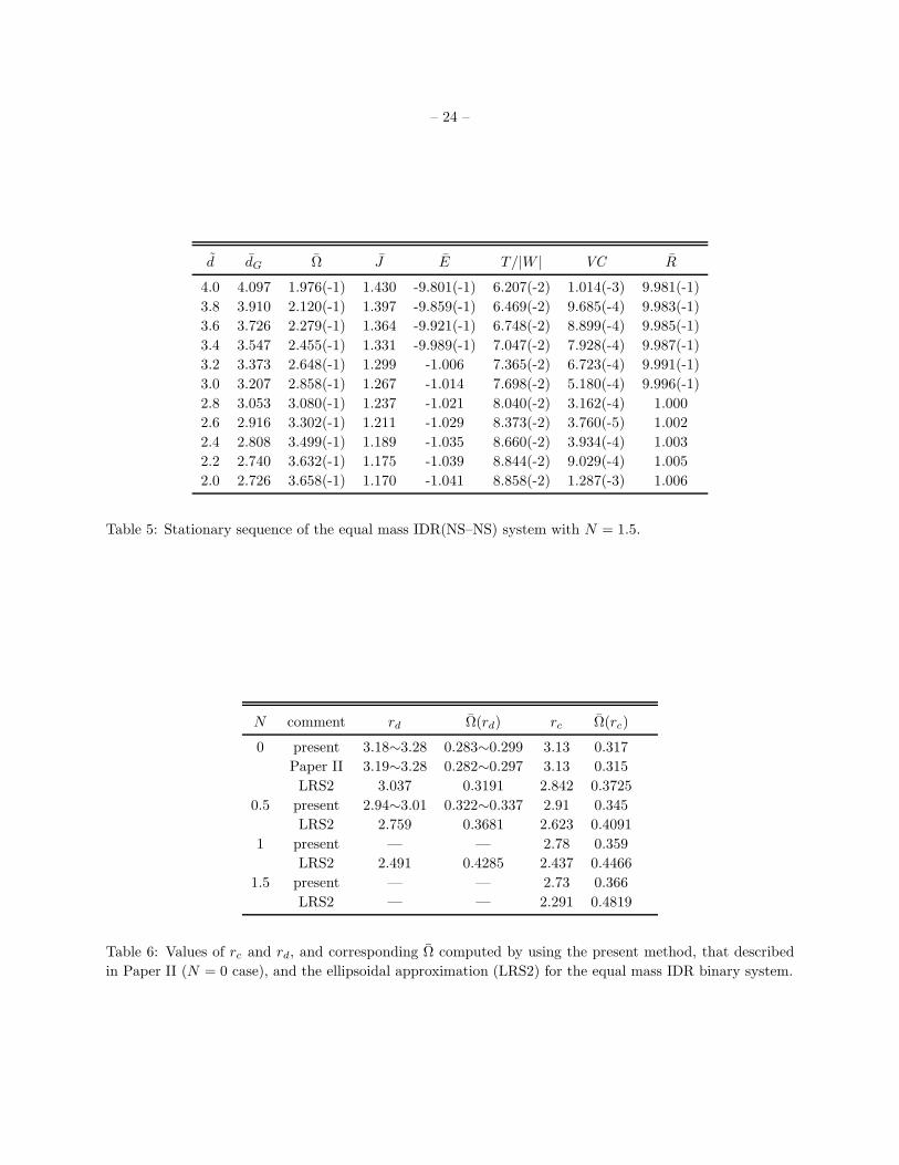
We have computed several equal mass IDR (NS–NS) sequences. In Tables 1-5, the physical quantities

are shown for sequences with polytropic indices N = 0, 0.5, 0.7, 1 and 1.5, respectively.

– 15 –

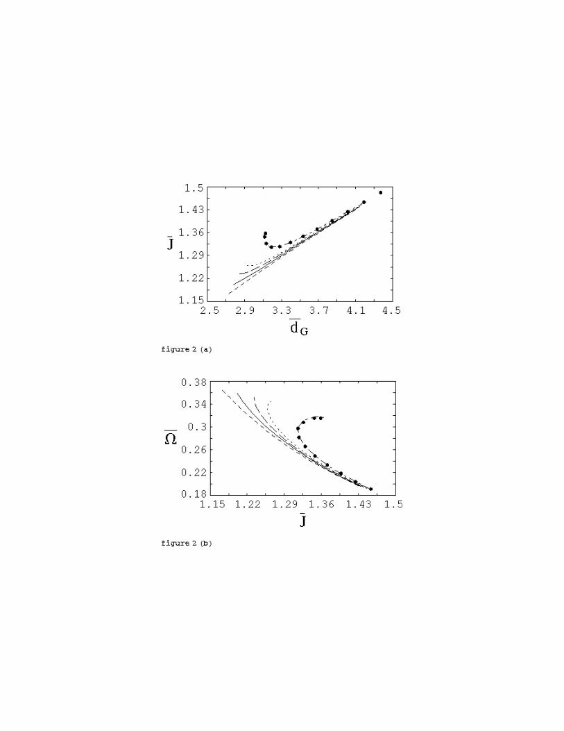
In order to check on the accuracy of our new numerical method, we compare our results with those

of LRS2 who used the ellipsoidal approximation which should be excellent at least when the separation is

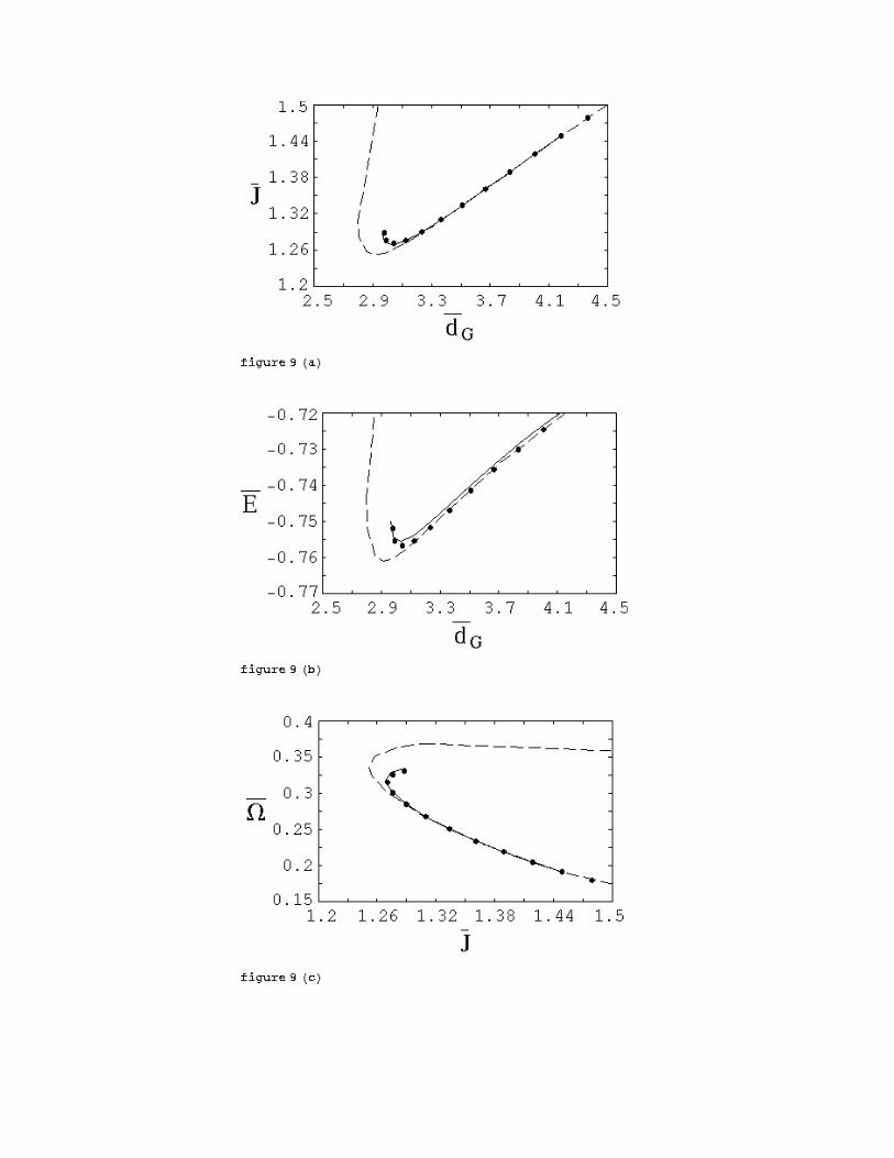
relatively large. In Figure 1, J(dG), E(dG) and Ω(J) are plotted for the N = 1.5 sequence. Similar figures

for the smaller values of polytropic indices N = 0, 0.5 and 1 are presented in Paper I. In this figure our

results for the N = 1.5 sequence agree well with those in LRS2 within a relative error less than 0.8% for

J(dG) and 0.4% for E(dG). This agreement with the LRS’s results shows that our method can accurately

compute configurations with any polytropic index as far as deformation is not far from ellipsoid. In

Figure 2, we draw J(dG) and Ω(J) for sequences with N = 0, 0.5, 0.7, 1 and 1.5. We also plot the results

of incompressible (N = 0) models computed by using a different formulation and a different solving method

described in Paper II. The results of N = 0 sequences computed by the present method and those obtained

in paper II coincide very well, although these two results are computed by using two totally independent

codes. This fact shows that our present computational code works accurately even for highly deformed

configurations. In particular, since our new code is accurate enough to resolve curves around the turning

point of J(dG) or E(dG) for N = 0 polytropes, we can expect that it will give precise behavior around

the critical separations for N 6= 0 polytropes as well. As discussed in Paper II, the point of the minimum

value of J(dG) or E(dG) does not appear along the binary sequence when the polytropic index satisfies the

condition N ∼> 0.7. Since the equation of state of realistic neutron stars is thought to be approximated

by polytropic equation of state with index 0.5 ∼ 1, there arises a possibility that in a new scenario of the

inspiraling neutron star binary in weak gravity limit, two component stars approach each other and finally

form a dumbbell like configuration before dynamical instability sets in.

As mentioned above and in Paper I, we have shown that dynamical instability limit disappears along

binary sequences for polytropes with N ∼> 0.7. We tabulate values of rd and rc of our results and those of

LRS2 for various polytropic indices in Table 6. Quantitative difference becomes larger as the polytropic

index N becomes larger. Even for smaller values as N ∼ 0.5, values of the angular velocity Ω(rd) differ by

∼ 10% or so between our present results and the results of LRS2. The difference of quantities at rc is much

larger. We will explain the reason why the ellipsoidal approximation cannot give precise values for rd or rcin below.

4.1.2. Binary configurations

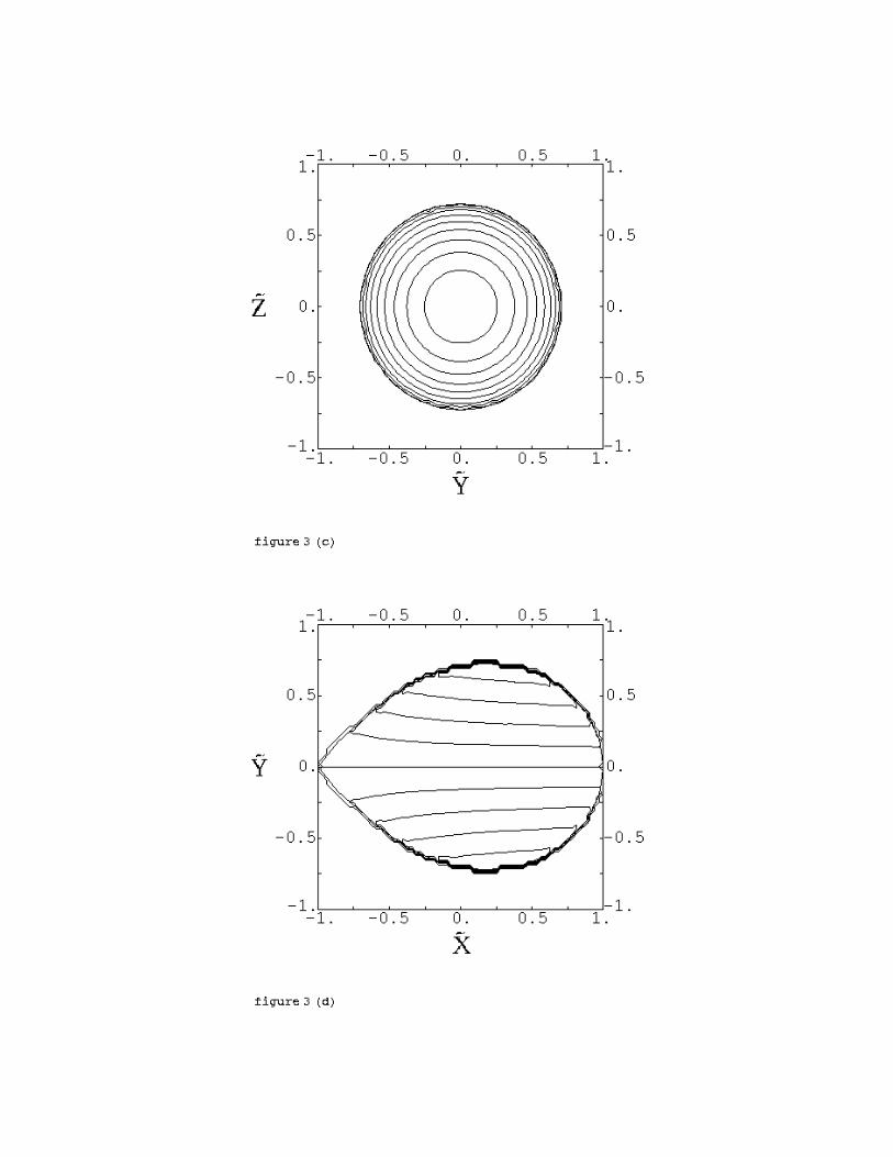
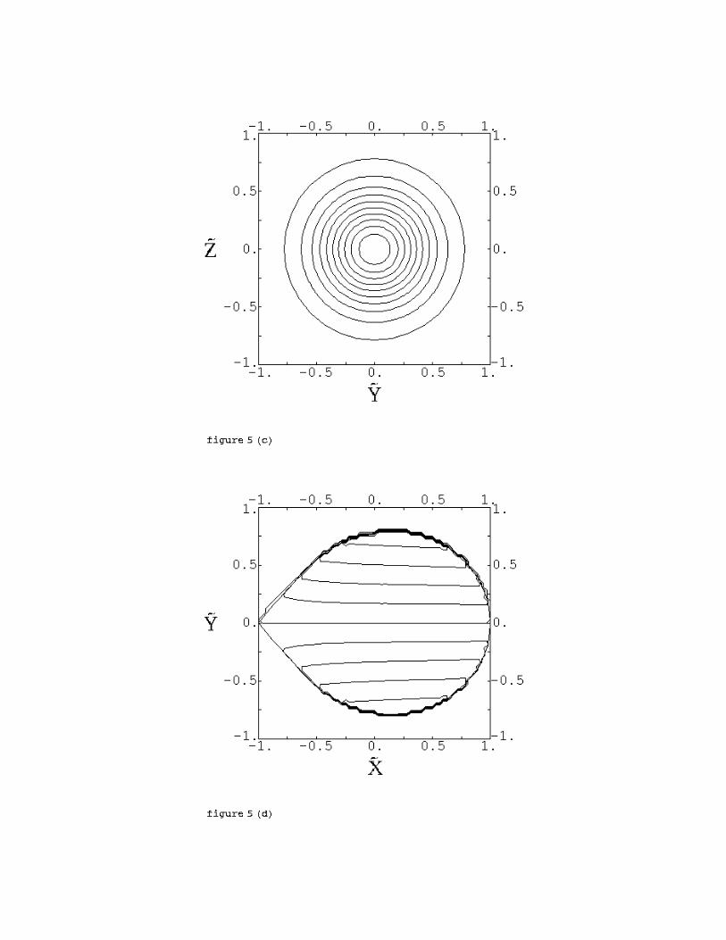
In Figures 3, 4 and 5, we show contours of the density and the velocity potential distributions for

N = 0.5, N = 1 and N = 1.5 polytropes in contact phases, respectively. It is noted that the configuration

with N = 0.5 in Figure 3 is dynamically unstable.

We can clearly see differences between the present results and those of the ellipsoidal approximation

from these figures. In general, the density distribution of a component star with a larger polytropic index

is centrally condensed, i.e. the star with a soft equation of state consists of a high density core and an

extended low density envelope. Although the central high density cores can be approximated well by the

ellipsoidal configurations, the extended envelopes of compressible gaseous stars deform from ellipsoidal

figures by tidal force of the other component. By comparing panels (a) and (b) in Figures 3, 4 and 5,

the location of the maximum density shifts to a larger value of x. It implies that the deformation of the

envelope due to the tidal force becomes large and that the inner parts of the envelopes come to contact

each other. Because of this significant deformation of the envelopes, two soft components stars contact

each other at a larger separation dG = rc than that for the ellipsoidal approximation. Therefore differences

between our results and those of LRS2 for rc or rd become significant.

– 16 –

The good agreement of our results and those of the ellipsoidal approximation as seen from Figure 1 can

be explained by using these density distributions as follows. First, since the mass content in the envelope is

very small, the contribution of the envelope to those quantities is very small. Furthermore, larger values of

rc means that the condensed core region becomes less affected from tidal force and consequently the shape

deforms little from an ellipsoidal figure. Therefore those quantities which are determined mainly from the

contribution of the core region coincide well with the results of the ellipsoidal approximation. It should be

noted, however, that precise values of rc or rd cannot be computed by the ellipsoidal approximation as

mentioned above.

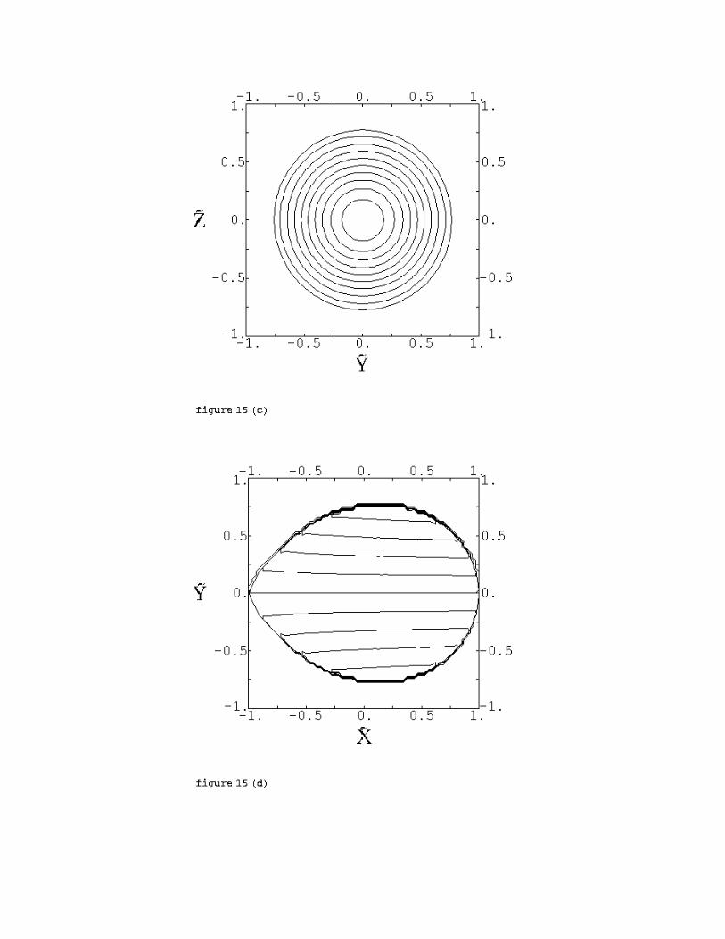
From panels (c) of these contours with several polytropic indices, we can see that the cross section

parallel to the y–z plane is slightly prolate, i.e. the radius along the axis Z is longer than that along the Y

axis. This difference of the radii is smaller for the star with larger polytropic indices. The cross section

becomes almost axisymmetric about the x–axis for polytropes with N = 1 and N = 1.5. Concerning the

velocity fields, we show distributions of the velocity potential in the figure (d) of each Figure. Since the

contour of the velocity potential seems almost paralell to z-axis i.e. z-independent, the velocity field is

almost plane parallel to equatorial plane and do not depend on z also.

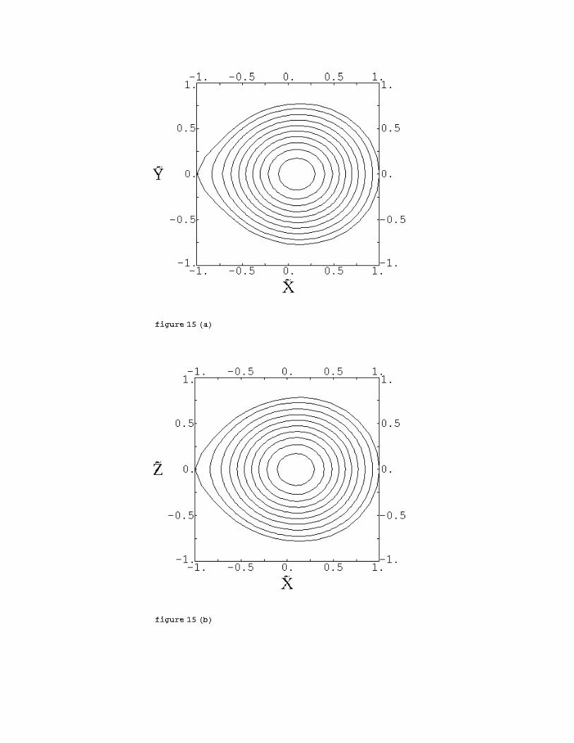
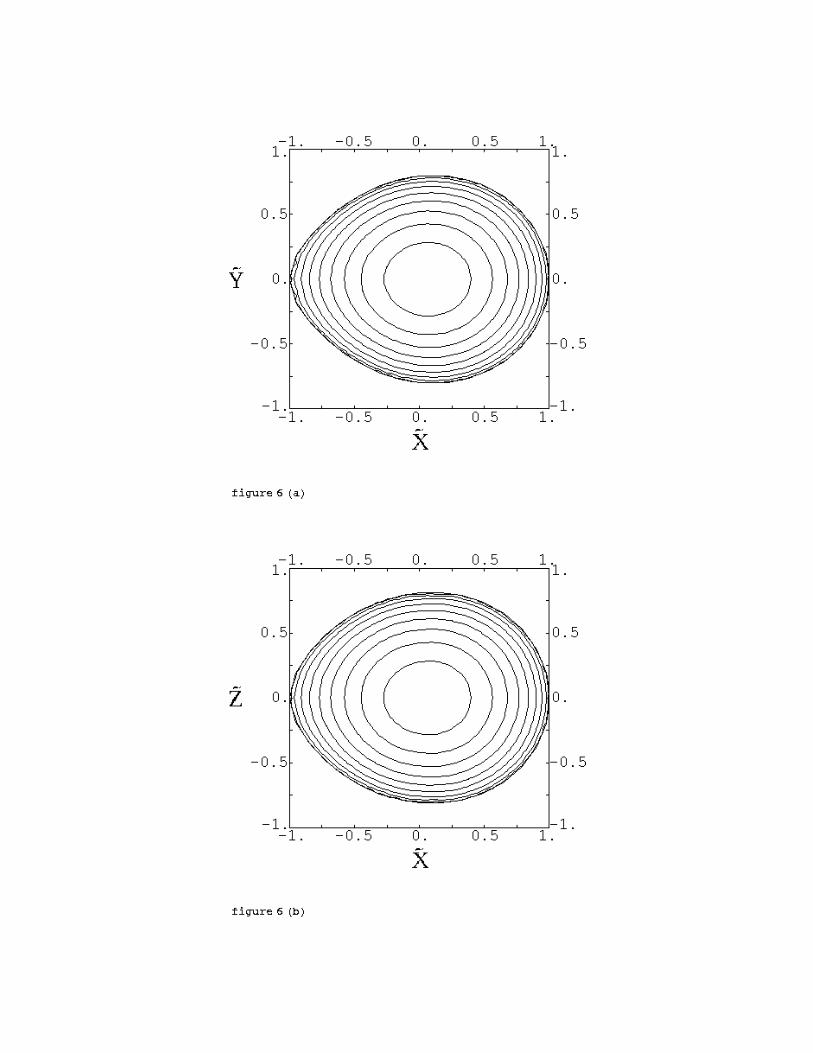
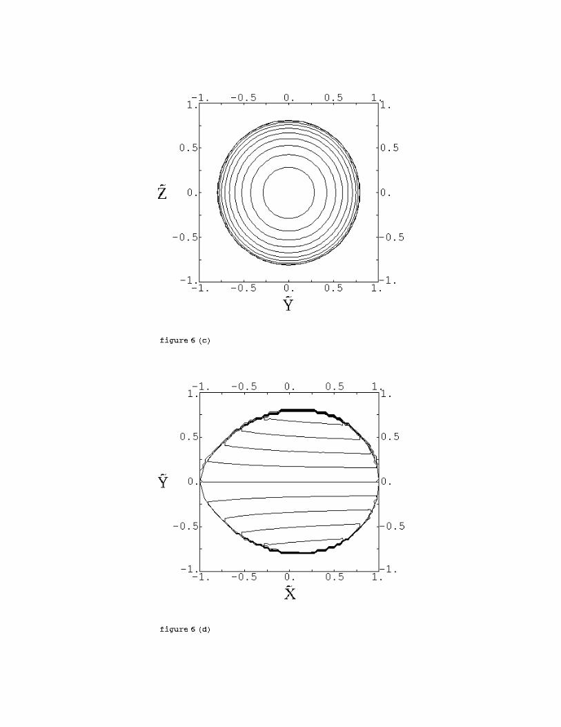
In Figure 6, we show the internal structure for N = 0.5 and d = 2.4 which almost corresponds to the

configuration at the dinamical instability limit rd. Different from Figures 3, 4 and 5, the shape of contours

in panels (a), (b) and (d) does not have a cusp, since two component stars are slightly detached. In

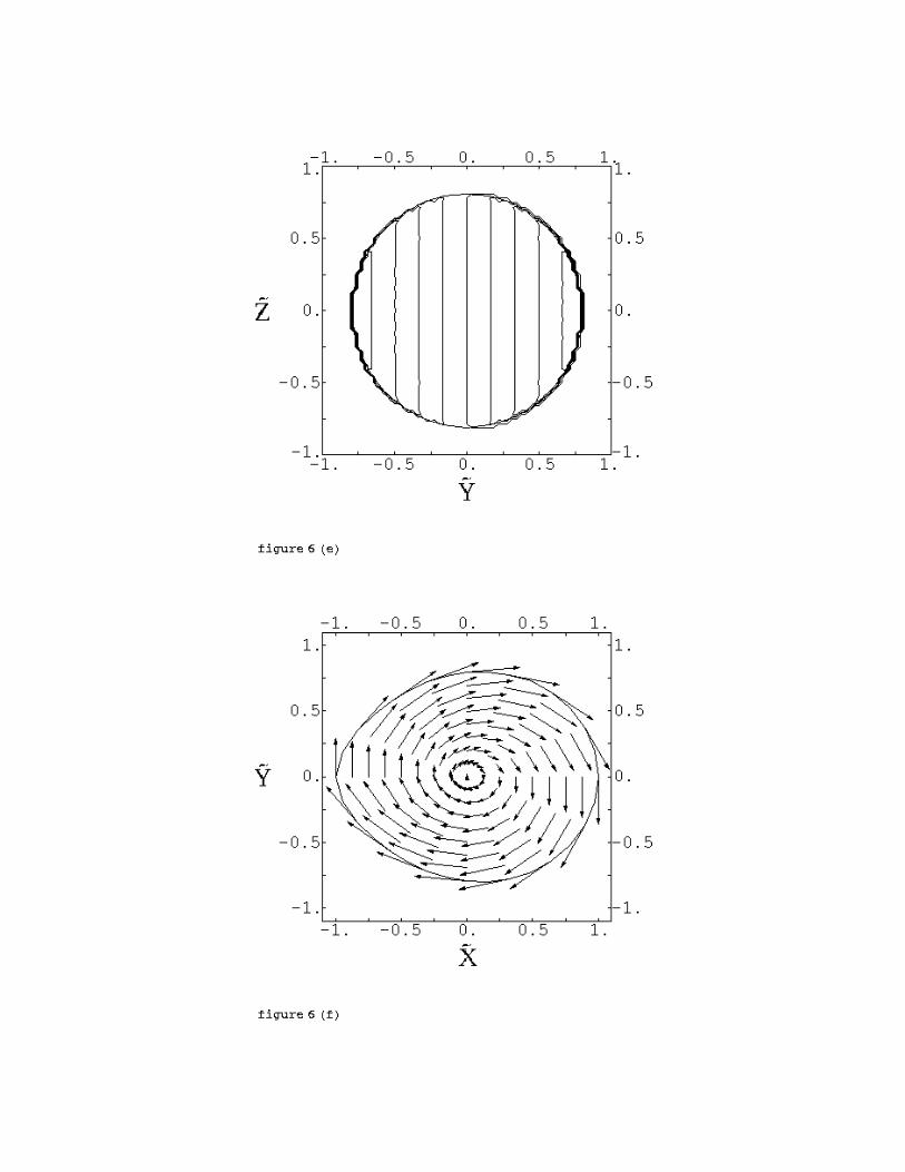
Figure 6 (e) contours of the velocity potential in the plane which is parallel to the y-z plane and intersects

with the geometrical center of the star are shown. As mentioned before, the velocity potential almost do

not depend on z. Therefore, we can consider that this figure expresses that the flow is almost planar, i.e.

parallel to the equatorial plane, and independent of z cooridnate. The stationary velocity field u in the

equatorial plane in the rotational frame is also shown in Figure 6 (f). The shapes of the star whose internal

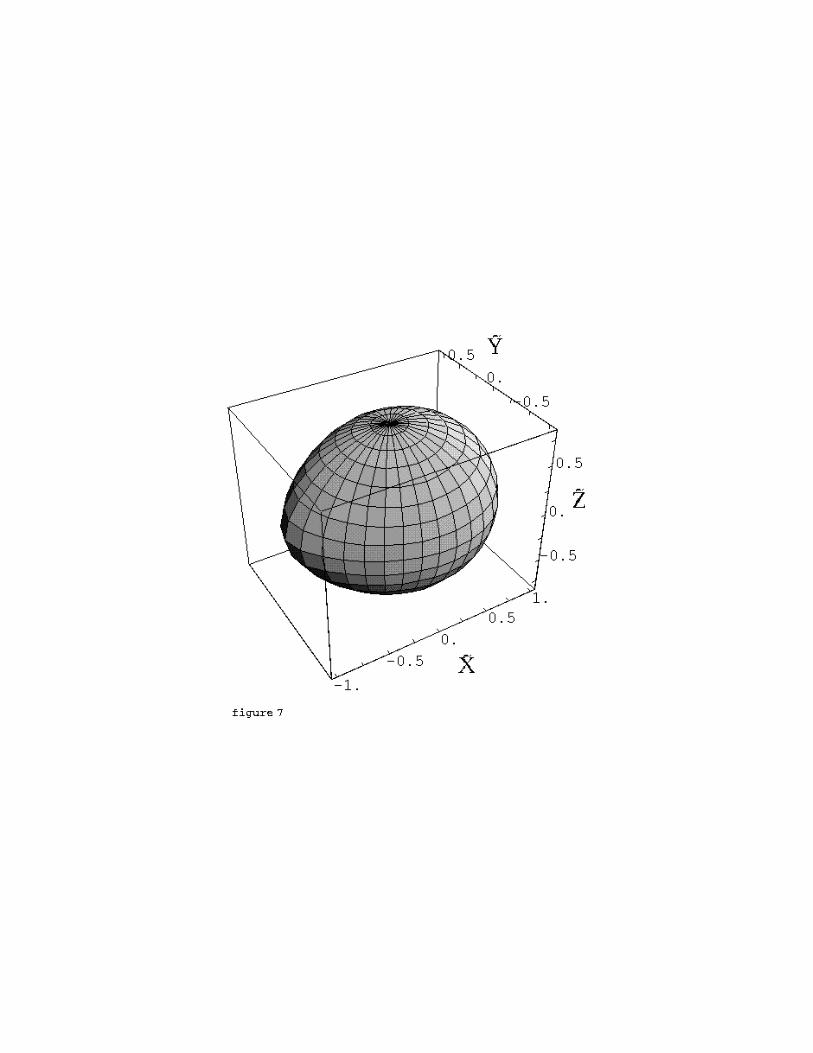
structures are shown in Figure 6 are displayed in Figure 7.

In Figure 8 (a) we show the velocity profile along the x-axis for the polytropes with N = 0, 0.5, 1

and 1.5 at contact phases, and also that for N = 0.5 polytropes at nearly the dynamical instability limit in

Figure 8 (b). Along the x-axis, there exists only the y-component of the velocity field vy in the Cartesian

coordinate. For synchronously rotating stars, vy is proportional to x, i.e. vy ∝ x, on the x-axis. On the

other hand, vy tends to a constant value at larger x for the irrotational binary systems. If we approximate

the distribution along the x-axis by vy ∝ xα + const, the exponent α is α ∼ 0.4 at the inner region and

α ∼ 0.1 at the outer region near the contact stage. The significant difference from synchronously rotating

binaries is that the velocity vy at x = 0 for the contact phase does not vanish but is finite. These differences

about the velocity fields will result in the different evolution from that of synchronously rotating binaries

after the contact or merging phase of two stars.

4.2. Compressible IRR binary systems with several mass ratios

4.2.1. Stationary sequences

We have computed IRR (BH–NS) sequences for several polytropic indices and several mass ratios.

In Tables 7-15, the physical quantities are shown for polytropic sequences with N = 0, 0.5 and 1 for

MNS/MBH = 1, 0.5 and 0.1 binaries, respectively.

In Figures 9 and 10, we show three different results for N = 0 polytropes: the results computed by our

– 17 –

present method, those of LRS1 and those obtained in Paper II. For equal mass sequences in Figure 9, our

present results agree very well with those of Paper II everywhere along the sequence down to the smallest

separation. Therefore, just as the IDR binary systems, our computational method will be able to give

accurate models for the contact binary systems with highly deformed stars around the critical radius. In

Figure 10, we can see a good agreement of our present results with other two results for the sequence with

MNS/MBH = 0.1. Since the mass of a point source MBH is dominant, deformation of a gaseous component

(NS) does not affect the physical quantities shown in those figures. Therefore three different results agree

well even near the critical separations. However the critical separations rd and rR of our present results

agree with those of Paper II but not with those of LRS1. Therefore the ellipsoidal approximation gives

different values for the critical separations again as is expected.

In Figures 11 and 12, we draw the sequences for N = 1 polytropes with MNS/MBH = 1 and 0.1,

respectively. In these figures, results by LRS1 are also shown. As seen from these figures, for polytropes

with larger N and/or larger MNS/MBH , two results agree each other everywhere. Even for smaller values

of N and MNS/MBH , these results are in good agreement for models with larger separations. Hence our

code for the IRR binary systems works accurately as that for the IDR binary systems as mentioned before.

In these figures, however, there are clear differences from those for N = 0 polytropes. In our present

calculations, the dynamical instability limit does not appear along the sequence with N = 1, i.e. both

J(dG) and E(dG) curves terminate at the smallest separation without reaching a turning point.

However we should note that situation for the IRR binary systems is different from that for the equal

mass IDR binary systems. For the equal mass IDR binary systems, the end point of the sequence exactly

corresponds to a configuration with d = 2. Thus we know rc a priori. However, for the IRR binary systems,

there exist sequences for which it is hard to find turning points along stationary sequences. This may occur

for models with larger mass difference, say MNS/MBH ∼ 0.1, because they have ‘shallow’ local minimum as

in Figure 10 (a) or (b). Consequently we need to compute the terminal point of the sequence by changing

the separation d carefully.

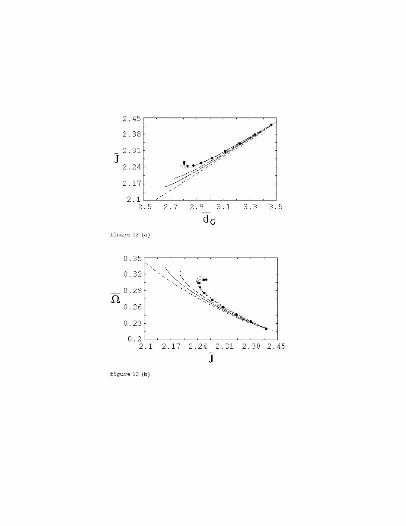
In Figure 13, we show the IRR sequences of polytropes with the same mass ratio MNS/MBH = 0.5

but with different polytropic indices N = 0, 0.1, 0.3, 0.5 and 1. The critical points of the sequences can

be found from these figures. Since the curves for smaller values of N show clearly the turning points of

J(dG) in Figure 13 (a), the sequences around the smallest separation have been considered reliable. We also

show the results of Paper II by dots as before which also show the accuracy of our present computations.

Figure 13 (a) reveals that the turning points disappear for N ∼> 0.6 polytropes and hence the sequence

directly reaches the Roche-Riemann limit with rR as the BH and the NS approach each other. The realistic

equation of state is considered to be included in this range of the polytropic index. These results suggest

a new scenario for the final fate of the IRR binary system evolution due to emission of GW. In the limit

of Newtonian gravity, the IRR binary systems will not become dynamically unstable before reaching the

Roche-Riemann limit with rR. Therefore the NS will not ‘fall on’ to the BH but the tidal disruption or

Roche overflow will happen. Systematic studies on the Roche limit rR and ISCO of the BH–NS system in

weak gravitational limit with various mass ratios should be considered in the subsequent paper (Uryu &

Eriguchi 1998c).

– 18 –

4.2.2. Binary configurations

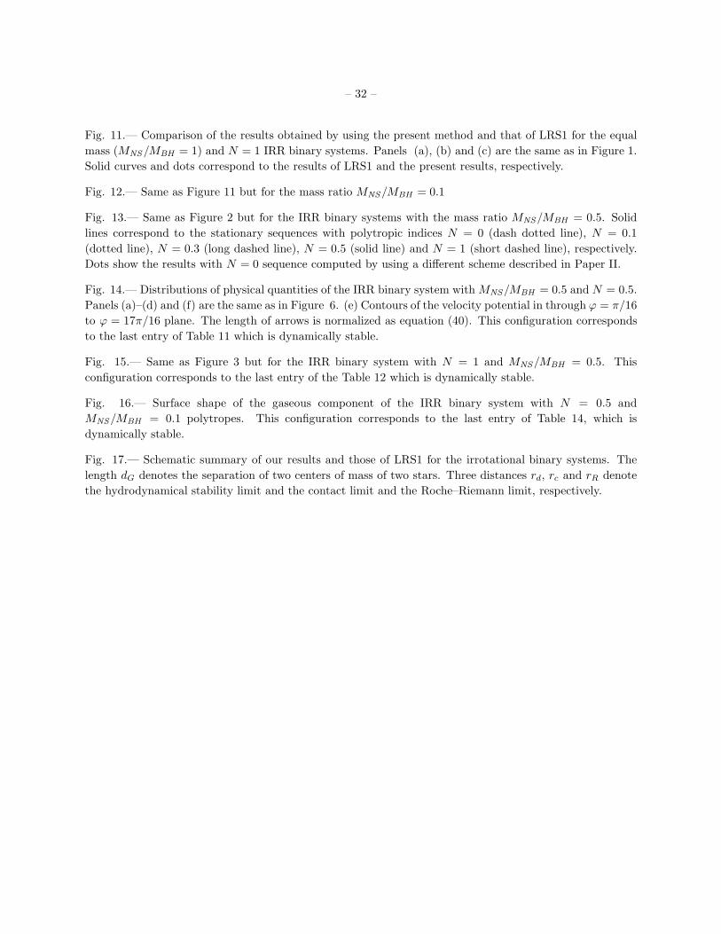
The compressible gaseous star components (NS) become highly deformed for larger mass ratios. In

Figures 14 and 15, contours of the density and the velocity potential distributions for binary systems with

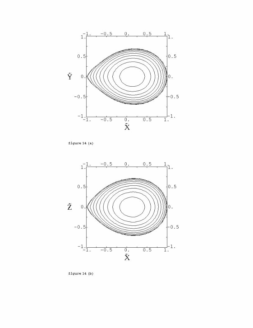
MNS/MBH = 0.5 are displayed for polytropic components with N = 0.5 and 1, respectively. They also

correspond to the models with the smallest separations tabulated in Tables 11 and 12, respectively. In

panels (a) and (b) of Figures 14 and 15, the density distributions in the equatorial and meridional sections

show that the inner edges of the stars become cusp-like. It should be noted that these configurations

are those of near the smallest separations and of dynamically stable models. They also show that the

configurations become slightly prolate for the IRR binary systems. The dependency of physical quantities

on the values of the polytropic index N is the same as that of the IDR systems. Consequently the curves

of J(dG) and E(dG) agree well with those of LRS but the critical distances rd and rR become different

from theirs. For the smaller MNS/MBH , the difference from the results of LRS becomes relatively smaller

because the point source with a larger mass determines the bulk structures and the quantities such as J(dG)

and E(dG).

In Figure 14(e), the distribution of the velocity potential in the ϕ = π/16 and ϕ = 17π/16 planes is

shown. We can see there is almost no z-dependence of Φ in these planes also as mentioned in the previous

section. In Figure 14 (f), the velocity field in the rotating frame u of the same model is drawn. Since the

density of the gas becomes relatively low near the inner edge of the star, the velocity becomes slower there

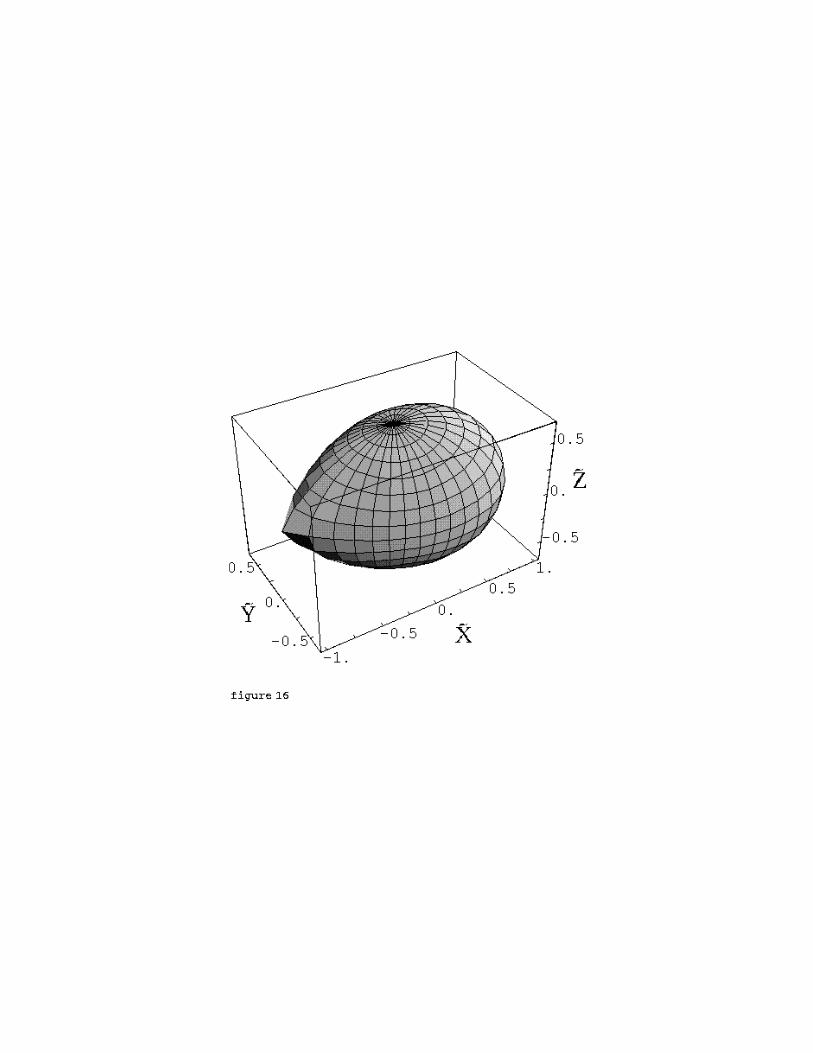
accordingly. In Figure 16, we show the shape of the surface of the model with N = 0.5 and MNS/MBH = 0.1

at the smallest separation displayed in Table 14.

5. Discussion

5.1. Equilibrium approach vs. dynamical simulation

In this paper we have presented a new numerical method based on a new formulation to compute the

irrotational gaseous binary systems and showed results for BH–NS and NS–NS binary systems in Newtonian

gravity.

There have been two different approaches to investigate realistic close binary systems which are

consist of compact objects : one is an equilibrium approach as presented in this paper and the other

is a dynamical approach such as simulations. Synchronously rotating NS–NS binary systems have been

studied by several authors by using equilibrium approaches. In particular, the ISCO have been investigated

under the post-Newtonian approximation (Shibata 1997) and by employing simplified general relativistic

formulation (Baumgarte et al. 1997c). However, for irrotational binary systems, only approximate solutions

have been investigated in the equilibrium approach (LRS2). Therefore our present method based on a new

formulation is the first attempt to treat stationary states of irrotational binary systems exactly, even though

Newtonian gravity is used.

On the other hand, several researchers have performed dynamical simulations for this problem. This

approach has been employed mainly from requirement of knowing wave forms of GW during dynamical

coalescence because they are crucial to extract information about the sources by comparing theoretical

predictions with observational results. In this approach, some authors have computed evolution of

synchronously rotating coalescing binary NS systems (Shibata, Nakamura & Oohara 1992; Shibata, Oohara

& Nakamura 1997; Rasio & Shapiro 1994 ; see also Rasio & Shapiro 1996). In particular, Rasio &

– 19 –

Shapiro (1994) and Shibata, Oohara & Nakamura (1997) constructed initial equilibrium configurations of

synchronously rotating binary systems accurately. By starting from such initial states, they carried out

dynamical evolutionary computations by using their hydrodynamical codes and compared their results with

other results which have been obtained by equilibrium approaches. Shibata, Oohara & Nakamura (1997)

have proceeded their computations up to the first post-Newtonian (1PN) hydrodynamical simulations

starting from equilibrium configurations of synchronously rotating binary systems obtained in the 1PN

approximation. They used the equilibrium configurations which have slightly larger and smaller separations

than rd as their initial conditions and checked whether those configurations are dynamically stable or not.

However, for non-synchronously rotating systems, computations using a dynamical approach are not

yet completely satisfactory because of very approximate initial configurations or having computations

which are not as accurate as for the synchronous models. (see for example, Shibata, Nakamura & Oohara

1992 ; Zhuge, Centrella & McMillan 1994, 1996; Davis et. al. 1994; Ruffert, Rampp & Janka 1997).

Shibata, Nakamura & Oohara (1992) tried to use two axisymmetrically rotating polytropes as their

initial configurations to approximate irrotationally spinning binary configurations. As mentioned in the

previous section, since the component stars of irrotational binary systems become slightly prolate, such

axisymmetric configurations are unsatisfactory. Zhuge, Centrella & McMillan (1994) and Ruffert, Rampp

& Janka (1997) have computed coalescence of non-synchronous binary systems by using approximate

irrotational configurations as their initial conditions. However it should be noted that their results have

not been carefully checked yet. Since the results of hydrodynamical simulations are very sensitive to

initial configurations and/or to numerical schemes, it is necessary to check whether those simulations are

as accurate as those of Rasio & Shapiro (1994) or Shibata, Oohara & Nakamura (1997). Therefore our

results of equilibrium approach will be important not only for checking the results of hydrodynamical

computations but also for providing reliable initial conditions for irrotational binary systems. Concerning

the IRR configurations, the dynamical simulation is recently performed by Lee & Kluzniak (1997). However,

detailed comparison of our results with theirs will be discussed in the subsequent paper (Uryu & Eriguchi

1998c).

5.2. Final stage of evolution for NS–NS or BH–NS binary systems

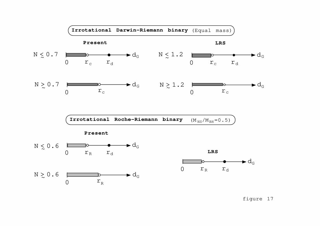
As discussed before, critical distances play an essential role in the final stage of binary evolution.

In Figure 17, we summarize our results and those of LRS1 for compressible irrotational binary systems

schematically. The upper part corresponds to the IDR binary systems with equal mass and the lower part

to the IRR binary systems with MNS/MBH = 0.5. In this figure arrows show the separations of two stars

for each sequence. Since the separation becomes smaller due to GW emission, the binary stars evolve from

the right to the left on each arrow, i.e. from a distant position to a position with a small distance. It should

be noted that, for relatively soft equations of state, the radius at which dynamical instability sets in does

not appear along the sequence from our numerical results. In particular, this is clear contrast to the results

of LRS who always found dynamically unstable limits for the IRR binary systems.

For the equal mass IDR binary systems, several numerical simulations show the formation of

dumbbell-like configurations (Shibata, Nakamura & Oohara 1992 ; Zhuge, Centrella & McMillan 1994 ;

Davis et. al. 1994 ; Ruffert, Rampp & Janka 1997). This can be explained by using the critical distances

as follows. Since the critical distance for the dynamical instability rd does not appear on the equal mass

NS–NS binary sequence for softer equations of state, the system evolves to the state with the critical radius

for the contact phase, i.e. rc. This can be also possible for the ellipsoidal models. However, the value of N is

– 20 –

much smaller for our exact numerical computations than that obtained from the ellipsoidal approximation.

It may be worth while considering evolution which will probably occur after contact of two stars. There

arises a difference from that for the synchronously rotating binary systems. Since irrotational stars have

non-zero velocity at the inner edge in the rotational frame at the contact stage as shown in Figure 6 (f), the

eddy may be excited and gases result in turbulence. Consequently complicated hydrodynamical phenomena

are expected to happen. Thus it is necessary to perform dynamical simulations with high resolution in

these regions (see e.g. Rasio & Shapiro 1996). Some detailed discussions of the effects due to realistic micro

physics of the coalescing NS–NS binary systems are given in Ruffert et al. (1997).

It is also important to investigate more realistic irrotational NS-NS in the framework of general

relativity (GR). Shibata (1997) has reported the GR effect on the synchronous NS–NS binary systems. He

obtained numerically exact configurations in post-Newtonian (PN) gravity. According to his results, the

effect weakens the tidal effect and hence the turning point of J(dG) or E(dG) disappears along the binary

sequence with the constant mass. Therefore it may be probable also for irrotational binary systems to reach

a contact phase without suffering from the dynamical instability when the GR effect is taken into account.

One of recent topics about merging of NS-NS binary systems is the numerical results obtained by

Wilson, Mathews & Marronetti (1996). They have involved a simplified GR effect and concluded that

individual neutron star in the binary system would collapse to form a BH on the circular orbit before

coalescence. Although this result has been criticized by many authors, they recently refute that such

phenomena can occur owing to the coupled effects of the spin of NS and the GR effect higher than 2PN

(see Mathews, Marronetti & Wilson 1997 and references there in). A definite answer to this conjecture may

be given by combining our method of irrotational binary systems and the GR treatment of gravity adopted

in Baumgarte et al. (1997c) for synchronously rotating systems by using the formulation of GR generalized

Bernoulli equation (Taub 1959 ; Bonazzola, Gourgoulhon & Marck 1997 ; Asada 1998 ; Shibata 1998 ;

Teukolsky 1998)

Concerning the IRR binary systems, situation is somewhat different from the IDR binary systems. As

described above, the ellipsoidal approximation shows that the critical radius rd always appears along the

binary sequence, i.e. rR < rd for any N . However, from our results, no dynamical instability limit along the

sequence appears for softer equations of state with N ∼> 0.6. This implies that neutron stars will not ‘fall

on’ to the BH but that the Roche lobe overflow may occur. Further discussion for IRR binary systems will

be presented in a subsequent paper (Uryu & Eriguchi 1998c).

To investigate more realistic final fates of BH-NS binary systems, we must further consider the radius

rGR at which GR instability sets in, i.e. the limit inside of which no stable orbits exist due to the effect

of strong gravity. Consequently, binary stars also fall down onto each other when two stars come within

rGR ∼ 6GMtot/c2. Although this critical distance rGR has not been treated in our present paper, we will be

able to implement the GR effect concerning the ISCO at rGR in our treatment of the Roche–Riemann type

binary systems by using the pseudo-Newtonian potential as was done by Taniguchi & Nakamura (1996). In

such a situation, the final fate of the BH–NS system will be determined by the positions of two lengths rRand rGR along the binary sequence. If we will be able to include the GR effect, we will find the position of

the radius rGR on this diagram 17 and clarify the final fate of the BH–NS systems.

We would like to thank Prof. J. C. Miller for carefully reading the manuscript and for helpful

comments. One of us (KU) also would like to thank Prof. D. W. Sciama and Dr. A. Lanza for their warm

hospitality at ICTP and SISSA. Numerical computations were carried out by at the Astronomical Data

– 21 –

Analysis Center of the National Astronomical Observatory, Japan.

– 22 –

d dG Ω J E T/|W | VC R

4.0 4.197 1.914(-1) 1.454 -1.316 8.347(-2) 6.777(-3) 9.994(-1)

3.8 4.022 2.043(-1) 1.425 -1.321 8.672(-2) 6.788(-3) 9.994(-1)

3.6 3.852 2.183(-1) 1.397 -1.326 9.019(-2) 6.828(-3) 9.994(-1)

3.4 3.690 2.335(-1) 1.371 -1.331 9.388(-2) 6.912(-3) 9.994(-1)

3.2 3.537 2.495(-1) 1.348 -1.336 9.782(-2) 6.960(-3) 9.994(-1)

3.0 3.399 2.662(-1) 1.329 -1.340 1.021(-1) 7.039(-3) 9.994(-1)

2.8 3.279 2.830(-1) 1.318 -1.343 1.068(-1) 7.218(-3) 9.994(-1)

2.6 3.184 2.985(-1) 1.315 -1.344 1.117(-1) 7.636(-3) 9.994(-1)

2.4 3.124 3.110(-1) 1.326 -1.341 1.168(-1) 8.117(-3) 9.994(-1)

2.2 3.107 3.181(-1) 1.350 -1.334 1.215(-1) 8.670(-3) 9.994(-1)

2.0 3.131 3.169(-1) 1.367 -1.330 1.227(-1) 9.209(-3) 9.994(-1)

Table 1: Stationary sequence of the equal mass IDR(NS–NS) system with N = 0. d is the separation of the

geometrical centers of two gaseous component stars (NS) which is defined as d = 2dNS/R0, where R0 is the

geometrical radius of the star along the x axis, that is R0 = (Rout − Rin)/2 (see equations (27) and (40)).

Other quantities are defined in equations (62), (66) and (67)

d dG Ω J E T/|W | VC R

4.0 4.165 1.933(-1) 1.446 -1.231 7.618(-2) 2.774(-2) 1.004

3.8 3.983 2.069(-1) 1.415 -1.236 7.925(-2) 2.751(-2) 1.004

3.6 3.804 2.219(-1) 1.385 -1.241 8.255(-2) 2.726(-2) 1.004

3.4 3.631 2.383(-1) 1.355 -1.247 8.608(-2) 2.699(-2) 1.004

3.2 3.466 2.560(-1) 1.327 -1.253 8.986(-2) 2.671(-2) 1.005

3.0 3.312 2.749(-1) 1.301 -1.259 9.385(-2) 2.638(-2) 1.005

2.8 3.172 2.944(-1) 1.280 -1.264 9.806(-2) 2.605(-2) 1.005

2.6 3.054 3.135(-1) 1.265 -1.268 1.025(-1) 2.581(-2) 1.006

2.5 3.005 3.223(-1) 1.260 -1.269 1.047(-1) 2.571(-2) 1.007

2.4 2.965 3.301(-1) 1.258 -1.270 1.068(-1) 2.558(-2) 1.008

2.3 2.935 3.366(-1) 1.258 -1.270 1.087(-1) 2.543(-2) 1.008

2.2 2.915 3.414(-1) 1.260 -1.269 1.103(-1) 2.533(-2) 1.009

2.0 2.906 3.447(-1) 1.265 -1.268 1.116(-1) 2.532(-2) 1.010

Table 2: Stationary sequence of the equal mass IDR(NS–NS) system with N = 0.5.

– 23 –

d dG Ω J E T/|W | VC R

4.0 4.141 1.949(-1) 1.440 -1.190 7.362(-2) 1.384(-2) 1.001

3.8 3.957 2.087(-1) 1.409 -1.196 7.662(-2) 1.370(-2) 1.001

3.6 3.778 2.239(-1) 1.378 -1.201 7.982(-2) 1.354(-2) 1.001

3.4 3.603 2.407(-1) 1.347 -1.208 8.325(-2) 1.337(-2) 1.001

3.2 3.436 2.589(-1) 1.318 -1.214 8.691(-2) 1.319(-2) 1.002

3.0 3.278 2.784(-1) 1.291 -1.220 9.079(-2) 1.297(-2) 1.002

2.8 3.135 2.986(-1) 1.267 -1.226 9.481(-2) 1.271(-2) 1.003

2.6 3.012 3.185(-1) 1.248 -1.231 9.890(-2) 1.246(-2) 1.004

2.4 2.917 3.360(-1) 1.237 -1.234 1.028(-1) 1.230(-2) 1.005

2.3 2.884 3.429(-1) 1.234 -1.235 1.045(-1) 1.219(-2) 1.006

2.2 2.861 3.481(-1) 1.233 -1.235 1.058(-1) 1.202(-2) 1.007

2.1 2.848 3.510(-1) 1.233 -1.235 1.066(-1) 1.187(-2) 1.007

2.0 2.847 3.515(-1) 1.233 -1.235 1.068(-1) 1.175(-2) 1.008

Table 3: Stationary sequence of the equal mass IDR(NS–NS) system with N = 0.7.

d dG Ω J E T/|W | VC R

4.0 4.119 1.962(-1) 1.435 -1.121 6.950(-2) 5.000(-3) 9.993(-1)

3.8 3.934 2.103(-1) 1.403 -1.127 7.235(-2) 4.911(-3) 9.994(-1)

3.6 3.753 2.259(-1) 1.371 -1.133 7.541(-2) 4.814(-3) 9.996(-1)

3.4 3.576 2.430(-1) 1.340 -1.139 7.869(-2) 4.709(-3) 9.998(-1)

3.2 3.405 2.618(-1) 1.309 -1.146 8.218(-2) 4.574(-3) 1.000

3.0 3.244 2.820(-1) 1.280 -1.153 8.585(-2) 4.416(-3) 1.001

2.8 3.095 3.032(-1) 1.253 -1.160 8.965(-2) 4.216(-3) 1.001

2.6 2.966 3.241(-1) 1.230 -1.166 9.341(-2) 3.946(-3) 1.002

2.4 2.864 3.427(-1) 1.213 -1.171 9.683(-2) 3.666(-3) 1.004

2.2 2.801 3.555(-1) 1.204 -1.1736 9.931(-2) 3.423(-3) 1.006

2.0 2.785 3.589(-1) 1.201 -1.1744 9.988(-2) 3.011(-3) 1.007

Table 4: Stationary sequence of the equal mass IDR(NS–NS) system with N = 1.

– 24 –

d dG Ω J E T/|W | VC R

4.0 4.097 1.976(-1) 1.430 -9.801(-1) 6.207(-2) 1.014(-3) 9.981(-1)

3.8 3.910 2.120(-1) 1.397 -9.859(-1) 6.469(-2) 9.685(-4) 9.983(-1)

3.6 3.726 2.279(-1) 1.364 -9.921(-1) 6.748(-2) 8.899(-4) 9.985(-1)

3.4 3.547 2.455(-1) 1.331 -9.989(-1) 7.047(-2) 7.928(-4) 9.987(-1)

3.2 3.373 2.648(-1) 1.299 -1.006 7.365(-2) 6.723(-4) 9.991(-1)

3.0 3.207 2.858(-1) 1.267 -1.014 7.698(-2) 5.180(-4) 9.996(-1)

2.8 3.053 3.080(-1) 1.237 -1.021 8.040(-2) 3.162(-4) 1.000

2.6 2.916 3.302(-1) 1.211 -1.029 8.373(-2) 3.760(-5) 1.002

2.4 2.808 3.499(-1) 1.189 -1.035 8.660(-2) 3.934(-4) 1.003

2.2 2.740 3.632(-1) 1.175 -1.039 8.844(-2) 9.029(-4) 1.005

2.0 2.726 3.658(-1) 1.170 -1.041 8.858(-2) 1.287(-3) 1.006

Table 5: Stationary sequence of the equal mass IDR(NS–NS) system with N = 1.5.

N comment rd Ω(rd) rc Ω(rc)

0 present 3.18∼3.28 0.283∼0.299 3.13 0.317

Paper II 3.19∼3.28 0.282∼0.297 3.13 0.315

LRS2 3.037 0.3191 2.842 0.3725

0.5 present 2.94∼3.01 0.322∼0.337 2.91 0.345

LRS2 2.759 0.3681 2.623 0.4091

1 present — — 2.78 0.359

LRS2 2.491 0.4285 2.437 0.4466

1.5 present — — 2.73 0.366

LRS2 — — 2.291 0.4819

Table 6: Values of rc and rd, and corresponding Ω computed by using the present method, that described

in Paper II (N = 0 case), and the ellipsoidal approximation (LRS2) for the equal mass IDR binary system.

– 25 –

d dG Ω J E T/|W | VC R

4.0 4.188 1.913(-1) 1.450 -7.180(-1) 1.429(-1) 5.789(-3) 9.994(-1)

3.8 4.010 2.042(-1) 1.419 -7.231(-1) 1.476(-1) 5.771(-3) 9.994(-1)

3.6 3.838 2.184(-1) 1.390 -7.285(-1) 1.525(-1) 5.755(-3) 9.994(-1)

3.4 3.671 2.337(-1) 1.361 -7.341(-1) 1.577(-1) 5.765(-3) 9.994(-1)

3.2 3.512 2.501(-1) 1.334 -7.399(-1) 1.630(-1) 5.818(-3) 9.994(-1)

3.0 3.365 2.673(-1) 1.310 -7.453(-1) 1.686(-1) 5.837(-3) 9.994(-1)

2.8 3.232 2.849(-1) 1.289 -7.501(-1) 1.746(-1) 5.841(-3) 9.994(-1)

2.6 3.119 3.020(-1) 1.275 -7.538(-1) 1.807(-1) 6.075(-3) 9.994(-1)

2.4 3.031 3.173(-1) 1.269 -7.555(-1) 1.870(-1) 6.457(-3) 9.994(-1)

2.2 2.977 3.288(-1) 1.274 -7.541(-1) 1.933(-1) 6.899(-3) 9.994(-1)

2.0 2.964 3.337(-1) 1.288 -7.501(-1) 1.980(-1) 7.425(-3) 9.994(-1)

Table 7: Stationary sequence of the IRR(BH–NS) system with MNS/MBH = 1 and N = 0. d is the

separation of a point source (BH) and the geometrical center of gaseous component star (NS) which is

defined as d = (dBH + dNS )/R0, where R0 is the geometrical radius of the star along the x axis, that is

R0 = (Rout −Rin)/2 (see equations (27) and (40)). Other quantities are defined in equations (62), (66) and

(67)

d dG Ω J E T/|W | VC R

4.0 4.159 1.932(-1) 1.443 -6.755(-1) 1.322(-1) 2.408(-2) 1.004

3.8 3.974 2.068(-1) 1.412 -6.809(-1) 1.368(-1) 2.376(-2) 1.004

3.6 3.794 2.219(-1) 1.380 -6.868(-1) 1.416(-1) 2.341(-2) 1.004

3.4 3.618 2.384(-1) 1.349 -6.930(-1) 1.467(-1) 2.304(-2) 1.004

3.2 3.449 2.565(-1) 1.318 -6.995(-1) 1.521(-1) 2.266(-2) 1.005

3.0 3.288 2.759(-1) 1.289 -7.061(-1) 1.577(-1) 2.223(-2) 1.005

2.8 3.140 2.962(-1) 1.263 -7.126(-1) 1.635(-1) 2.181(-2) 1.006

2.6 3.010 3.166(-1) 1.241 -7.184(-1) 1.694(-1) 2.145(-2) 1.006

2.4 2.904 3.354(-1) 1.226 -7.227(-1) 1.752(-1) 2.108(-2) 1.008

2.2 2.834 3.495(-1) 1.219 -7.248(-1) 1.801(-1) 2.071(-2) 1.009

Table 8: Stationary sequence of the IRR(BH–NS) system with MNS/MBH = 1 and N = 0.5.

– 26 –

d dG Ω J E T/|W | VC R

4.0 4.114 1.962(-1) 1.434 -6.216(-1) 1.221(-1) 4.394(-3) 9.993(-1)

3.8 3.927 2.103(-1) 1.402 -6.273(-1) 1.265(-1) 4.299(-3) 9.994(-1)

3.6 3.744 2.261(-1) 1.369 -6.335(-1) 1.312(-1) 4.193(-3) 9.996(-1)

3.4 3.565 2.434(-1) 1.336 -6.401(-1) 1.361(-1) 4.073(-3) 9.998(-1)

3.2 3.391 2.625(-1) 1.304 -6.471(-1) 1.413(-1) 3.932(-3) 1.000

3.0 3.225 2.833(-1) 1.273 -6.545(-1) 1.467(-1) 3.772(-3) 1.001

2.8 3.070 3.053(-1) 1.243 -6.621(-1) 1.523(-1) 3.577(-3) 1.001

2.6 2.931 3.277(-1) 1.217 -6.693(-1) 1.577(-1) 3.310(-3) 1.003

2.4 2.818 3.482(-1) 1.196 -6.755(-1) 1.628(-1) 3.053(-3) 1.004

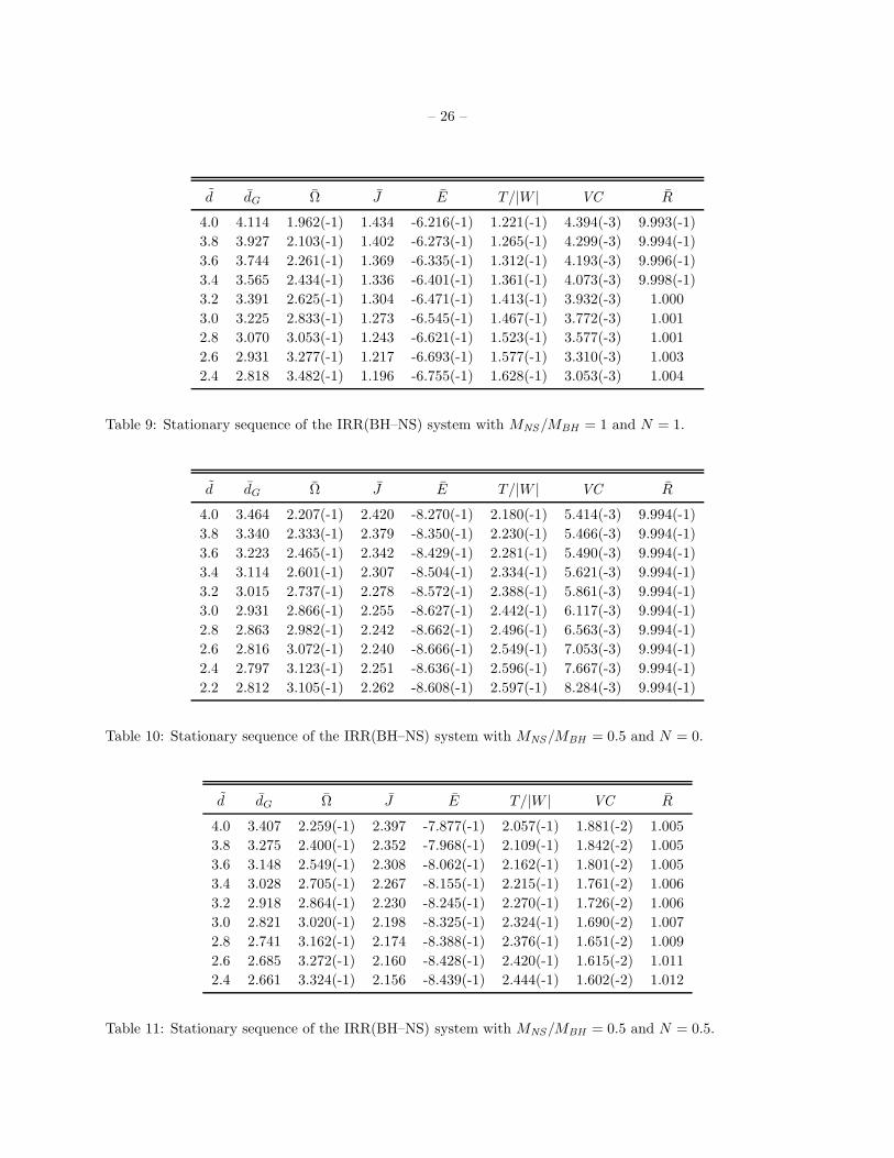
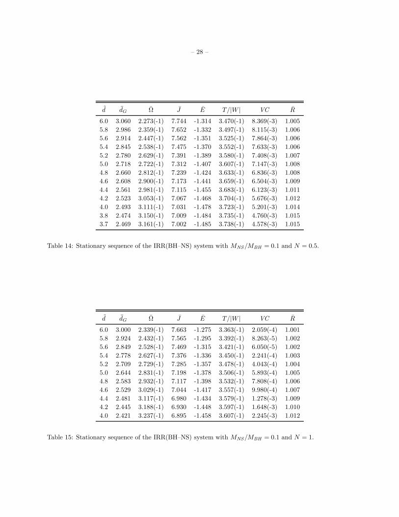
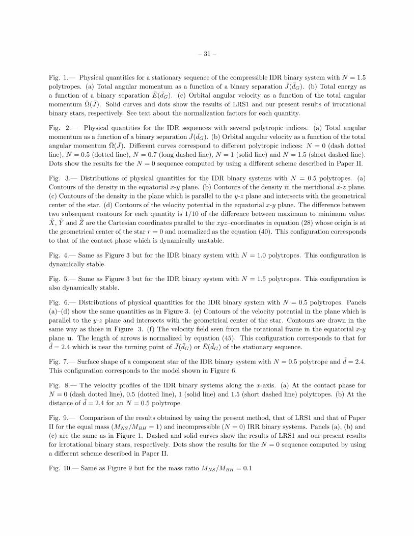
Table 9: Stationary sequence of the IRR(BH–NS) system with MNS/MBH = 1 and N = 1.

d dG Ω J E T/|W | VC R

4.0 3.464 2.207(-1) 2.420 -8.270(-1) 2.180(-1) 5.414(-3) 9.994(-1)

3.8 3.340 2.333(-1) 2.379 -8.350(-1) 2.230(-1) 5.466(-3) 9.994(-1)

3.6 3.223 2.465(-1) 2.342 -8.429(-1) 2.281(-1) 5.490(-3) 9.994(-1)

3.4 3.114 2.601(-1) 2.307 -8.504(-1) 2.334(-1) 5.621(-3) 9.994(-1)

3.2 3.015 2.737(-1) 2.278 -8.572(-1) 2.388(-1) 5.861(-3) 9.994(-1)

3.0 2.931 2.866(-1) 2.255 -8.627(-1) 2.442(-1) 6.117(-3) 9.994(-1)

2.8 2.863 2.982(-1) 2.242 -8.662(-1) 2.496(-1) 6.563(-3) 9.994(-1)

2.6 2.816 3.072(-1) 2.240 -8.666(-1) 2.549(-1) 7.053(-3) 9.994(-1)

2.4 2.797 3.123(-1) 2.251 -8.636(-1) 2.596(-1) 7.667(-3) 9.994(-1)

2.2 2.812 3.105(-1) 2.262 -8.608(-1) 2.597(-1) 8.284(-3) 9.994(-1)

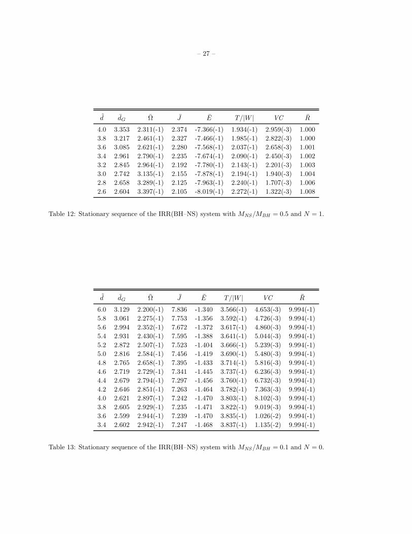
Table 10: Stationary sequence of the IRR(BH–NS) system with MNS/MBH = 0.5 and N = 0.

d dG Ω J E T/|W | VC R

4.0 3.407 2.259(-1) 2.397 -7.877(-1) 2.057(-1) 1.881(-2) 1.005

3.8 3.275 2.400(-1) 2.352 -7.968(-1) 2.109(-1) 1.842(-2) 1.005

3.6 3.148 2.549(-1) 2.308 -8.062(-1) 2.162(-1) 1.801(-2) 1.005

3.4 3.028 2.705(-1) 2.267 -8.155(-1) 2.215(-1) 1.761(-2) 1.006

3.2 2.918 2.864(-1) 2.230 -8.245(-1) 2.270(-1) 1.726(-2) 1.006

3.0 2.821 3.020(-1) 2.198 -8.325(-1) 2.324(-1) 1.690(-2) 1.007

2.8 2.741 3.162(-1) 2.174 -8.388(-1) 2.376(-1) 1.651(-2) 1.009

2.6 2.685 3.272(-1) 2.160 -8.428(-1) 2.420(-1) 1.615(-2) 1.011

2.4 2.661 3.324(-1) 2.156 -8.439(-1) 2.444(-1) 1.602(-2) 1.012

Table 11: Stationary sequence of the IRR(BH–NS) system with MNS/MBH = 0.5 and N = 0.5.

– 27 –

d dG Ω J E T/|W | VC R

4.0 3.353 2.311(-1) 2.374 -7.366(-1) 1.934(-1) 2.959(-3) 1.000

3.8 3.217 2.461(-1) 2.327 -7.466(-1) 1.985(-1) 2.822(-3) 1.000

3.6 3.085 2.621(-1) 2.280 -7.568(-1) 2.037(-1) 2.658(-3) 1.001

3.4 2.961 2.790(-1) 2.235 -7.674(-1) 2.090(-1) 2.450(-3) 1.002

3.2 2.845 2.964(-1) 2.192 -7.780(-1) 2.143(-1) 2.201(-3) 1.003

3.0 2.742 3.135(-1) 2.155 -7.878(-1) 2.194(-1) 1.940(-3) 1.004

2.8 2.658 3.289(-1) 2.125 -7.963(-1) 2.240(-1) 1.707(-3) 1.006

2.6 2.604 3.397(-1) 2.105 -8.019(-1) 2.272(-1) 1.322(-3) 1.008

Table 12: Stationary sequence of the IRR(BH–NS) system with MNS/MBH = 0.5 and N = 1.

d dG Ω J E T/|W | VC R

6.0 3.129 2.200(-1) 7.836 -1.340 3.566(-1) 4.653(-3) 9.994(-1)

5.8 3.061 2.275(-1) 7.753 -1.356 3.592(-1) 4.726(-3) 9.994(-1)

5.6 2.994 2.352(-1) 7.672 -1.372 3.617(-1) 4.860(-3) 9.994(-1)

5.4 2.931 2.430(-1) 7.595 -1.388 3.641(-1) 5.044(-3) 9.994(-1)

5.2 2.872 2.507(-1) 7.523 -1.404 3.666(-1) 5.239(-3) 9.994(-1)

5.0 2.816 2.584(-1) 7.456 -1.419 3.690(-1) 5.480(-3) 9.994(-1)

4.8 2.765 2.658(-1) 7.395 -1.433 3.714(-1) 5.816(-3) 9.994(-1)

4.6 2.719 2.729(-1) 7.341 -1.445 3.737(-1) 6.236(-3) 9.994(-1)

4.4 2.679 2.794(-1) 7.297 -1.456 3.760(-1) 6.732(-3) 9.994(-1)

4.2 2.646 2.851(-1) 7.263 -1.464 3.782(-1) 7.363(-3) 9.994(-1)

4.0 2.621 2.897(-1) 7.242 -1.470 3.803(-1) 8.102(-3) 9.994(-1)

3.8 2.605 2.929(-1) 7.235 -1.471 3.822(-1) 9.019(-3) 9.994(-1)

3.6 2.599 2.944(-1) 7.239 -1.470 3.835(-1) 1.026(-2) 9.994(-1)

3.4 2.602 2.942(-1) 7.247 -1.468 3.837(-1) 1.135(-2) 9.994(-1)

Table 13: Stationary sequence of the IRR(BH–NS) system with MNS/MBH = 0.1 and N = 0.

– 28 –

d dG Ω J E T/|W | VC R

6.0 3.060 2.273(-1) 7.744 -1.314 3.470(-1) 8.369(-3) 1.005

5.8 2.986 2.359(-1) 7.652 -1.332 3.497(-1) 8.115(-3) 1.006

5.6 2.914 2.447(-1) 7.562 -1.351 3.525(-1) 7.864(-3) 1.006

5.4 2.845 2.538(-1) 7.475 -1.370 3.552(-1) 7.633(-3) 1.006

5.2 2.780 2.629(-1) 7.391 -1.389 3.580(-1) 7.408(-3) 1.007

5.0 2.718 2.722(-1) 7.312 -1.407 3.607(-1) 7.147(-3) 1.008

4.8 2.660 2.812(-1) 7.239 -1.424 3.633(-1) 6.836(-3) 1.008

4.6 2.608 2.900(-1) 7.173 -1.441 3.659(-1) 6.504(-3) 1.009

4.4 2.561 2.981(-1) 7.115 -1.455 3.683(-1) 6.123(-3) 1.011

4.2 2.523 3.053(-1) 7.067 -1.468 3.704(-1) 5.676(-3) 1.012

4.0 2.493 3.111(-1) 7.031 -1.478 3.723(-1) 5.201(-3) 1.014

3.8 2.474 3.150(-1) 7.009 -1.484 3.735(-1) 4.760(-3) 1.015

3.7 2.469 3.161(-1) 7.002 -1.485 3.738(-1) 4.578(-3) 1.015

Table 14: Stationary sequence of the IRR(BH–NS) system with MNS/MBH = 0.1 and N = 0.5.

d dG Ω J E T/|W | VC R

6.0 3.000 2.339(-1) 7.663 -1.275 3.363(-1) 2.059(-4) 1.001

5.8 2.924 2.432(-1) 7.565 -1.295 3.392(-1) 8.263(-5) 1.002

5.6 2.849 2.528(-1) 7.469 -1.315 3.421(-1) 6.050(-5) 1.002

5.4 2.778 2.627(-1) 7.376 -1.336 3.450(-1) 2.241(-4) 1.003

5.2 2.709 2.729(-1) 7.285 -1.357 3.478(-1) 4.043(-4) 1.004

5.0 2.644 2.831(-1) 7.198 -1.378 3.506(-1) 5.893(-4) 1.005

4.8 2.583 2.932(-1) 7.117 -1.398 3.532(-1) 7.808(-4) 1.006

4.6 2.529 3.029(-1) 7.044 -1.417 3.557(-1) 9.980(-4) 1.007

4.4 2.481 3.117(-1) 6.980 -1.434 3.579(-1) 1.278(-3) 1.009

4.2 2.445 3.188(-1) 6.930 -1.448 3.597(-1) 1.648(-3) 1.010

4.0 2.421 3.237(-1) 6.895 -1.458 3.607(-1) 2.245(-3) 1.012

Table 15: Stationary sequence of the IRR(BH–NS) system with MNS/MBH = 0.1 and N = 1.

– 29 –

REFERENCES

Abramovici A. et al., 1992, Science, 256, 325

Aizenman M. L., 1968, ApJ, 153, 511

Asada .H, 1998, Phys. Rev. D, in press, (gr-qc/9804003)

Baumgarte T. W., Cook G. B., Scheel M. A., Shapiro S. L., Teukolsky S. A., 1997a, Phys. Rev. Lett., 79,

1182-1185, (gr-qc/9704024)

Baumgarte T. W., Cook G. B., Scheel M. A., Shapiro S. L., Teukolsky S. A., 1997b, Phys. Rev. Lett.,

submitted, (gr-qc/9705023)

Baumgarte T. W., Cook G. B., Scheel M. A., Shapiro S. L., Teukolsky S. A., 1997c, Phys. Rev. D,

submitted, (gr-qc/9709026)

Bildsten L., Cutler C., 1992, ApJ, 400, 175

Bonazzola S., Gourgoulhon E., Marck J.-A., 1997, Phys. Rev. D, in press (gr-qc/9710031)

Chandrasekhar S., 1969, Ellipsoidal Figures of Equilibrium, Yale University Press, New Haven

Davis M., Benz W., Piran T., Thielemann F., 1994, ApJ, 431, 742

Eriguchi Y., 1990, A&A, 229, 457

Eriguchi Y., Hachisu I., 1983, Prog. Theor. Phys., 70, 1534

Eriguchi Y., Hachisu I., 1985, A&A, 142, 256

Eriguchi Y., Muller E., 1985, A&A, 146, 260

Eriguchi Y., Futamase T., Hachisu I., 1990, A&A, 231, 61

Eriguchi Y., Hachisu I., Sugimoto D., 1982, Prog. Theor. Phys., 67, 1068

Hachisu I., 1986, ApJS, 62, 461

Hachisu I., Eriguchi Y., 1984a, PASJ, 36, 239

Hachisu I., Eriguchi Y., 1984b, PASJ, 36, 259

Kochanek C. S., 1992, ApJ, 398, 234

Komatsu H., Eriguchi Y. Hachisu I., 1989, MNRAS, 237, 355

Lai D., Rasio F. A., Shapiro S. L., 1993a, ApJ, 406, L63

Lai D., Rasio F. A., Shapiro S. L., 1993b, ApJS, 88, 205, LRS1

Lai D., Rasio F. A., Shapiro S. L., 1994a, ApJ, 420, 811, LRS2

Lai D., Rasio F. A., Shapiro S. L., 1994b, ApJ, 423, 344

Lombardi J. C., Rasio F. A., Shapiro S. L., 1997, Phys. Rev. D, 56, 3416

– 30 –

Lee W. H., Kluzniak W., 1997, in preparation

Mathews G .J., Marronetti P., Wilson J.R., 1997, Phys. Rev. D, submitted, (gr-qc/9710140)

Miller B.D., 1974, ApJ, 187, 609

Ostriker J. P., Mark J. W-K., 1968, ApJ, 151, 1075

Paczynski B., 1986, ApJ, 308, L43

Rasio F. A., Shapiro S. L., 1994, ApJ, 432, 242

Rasio F. A., Shapiro S. L., 1996, in Compact Stars in Binaries, proceedings of IAU Symposium 165, eds.

van Paradijs J., van den Heuvel E. P. J., Kuulkers E., Dordrecht, Kluwer Academic Publishers,

(astro-ph/9410085)

Ruffert M., Rampp M., Janka H.-T., 1997, A&A, 321, 991

Ruffert M., Janka H.-T., Takahashi K., Schaefer G., 1997, A&A, 319, 122

Shapiro S. L., Teukolsky S. A., 1983, Black Holes, White Dwarfs and Neutron Stars, Wiley, New York

Shibata M., 1997, Phys. Rev. D, 55, 6019

Shibata M., 1998, Phys. Rev. D, in press, (gr-qc/9803085)

Shibata M., Nakamura. T., Oohara K., 1992, Prog. Theor. Phys., 88, 1079

Shibata M., Oohara K., Nakamura. T., 1997, Prog. Theor. Phys., 98, in press

Taniguchi K., Nakamura T., 1996, Prog. Theor. Phys., 96, 693

Tassoul J.-L., 1978, Theory of Rotating Stars, Princeton Univ. Press, Princeton

Taub A. H., 1959, Arch. Ratl. Mech. Anal., 3, 312

Teukolsky S. A., 1998, ApJ, in press, (gr-qc/9803082)

Thorne K. S., 1994, in “Relativistic Cosmology” Proceedings of the 8-th Nishinomiya-Yukawa Memorial

Symposium, ed. Sasaki M., Universal Academy Press, Tokyo, p. 67

Uryu K., Eriguchi Y., 1996, MNRAS, 282, 653

Uryu K., Eriguchi Y., 1998a, MNRAS, 296, L1, Paper I (astro-ph/9712203)

Uryu K., Eriguchi Y., 1998b, MNRAS, in press, Paper II

Uryu K., Eriguchi Y., 1998c, in preparation

Wilson J .R., Mathews G .J., Marronetti P., 1996, Phys. Rev. D54, 1317

Yoshida S., Eriguchi Y., 1997, Phys. Rev. D56, 762

Zhuge X., Centrella J. M., McMillan S. L. W., 1994, Phys. Rev. D50, 6247

Zhuge X., Centrella J. M., McMillan S. L. W., 1996, Phys. Rev. D54, 7261

This preprint was prepared with the AAS LATEX macros v4.0.

– 31 –

Fig. 1.— Physical quantities for a stationary sequence of the compressible IDR binary system with N = 1.5

polytropes. (a) Total angular momentum as a function of a binary separation J(dG). (b) Total energy as

a function of a binary separation E(dG). (c) Orbital angular velocity as a function of the total angular

momentum Ω(J). Solid curves and dots show the results of LRS1 and our present results of irrotational

binary stars, respectively. See text about the normalization factors for each quantity.

Fig. 2.— Physical quantities for the IDR sequences with several polytropic indices. (a) Total angular

momentum as a function of a binary separation J(dG). (b) Orbital angular velocity as a function of the total

angular momentum Ω(J). Different curves correspond to different polytropic indices: N = 0 (dash dotted

line), N = 0.5 (dotted line), N = 0.7 (long dashed line), N = 1 (solid line) and N = 1.5 (short dashed line).

Dots show the results for the N = 0 sequence computed by using a different scheme described in Paper II.

Fig. 3.— Distributions of physical quantities for the IDR binary systems with N = 0.5 polytropes. (a)

Contours of the density in the equatorial x-y plane. (b) Contours of the density in the meridional x-z plane.

(c) Contours of the density in the plane which is parallel to the y-z plane and intersects with the geometrical

center of the star. (d) Contours of the velocity potential in the equatorial x-y plane. The difference between

two subsequent contours for each quantity is 1/10 of the difference between maximum to minimum value.

X, Y and Z are the Cartesian coordinates parallel to the xyz–coordinates in equation (28) whose origin is at

the geometrical center of the star r = 0 and normalized as the equation (40). This configuration corresponds

to that of the contact phase which is dynamically unstable.

Fig. 4.— Same as Figure 3 but for the IDR binary system with N = 1.0 polytropes. This configuration is

dynamically stable.

Fig. 5.— Same as Figure 3 but for the IDR binary system with N = 1.5 polytropes. This configuration is

also dynamically stable.

Fig. 6.— Distributions of physical quantities for the IDR binary system with N = 0.5 polytropes. Panels

(a)–(d) show the same quantities as in Figure 3. (e) Contours of the velocity potential in the plane which is

parallel to the y-z plane and intersects with the geometrical center of the star. Contours are drawn in the

same way as those in Figure 3. (f) The velocity field seen from the rotational frame in the equatorial x-y

plane u. The length of arrows is normalized by equation (45). This configuration corresponds to that for

d = 2.4 which is near the turning point of J(dG) or E(dG) of the stationary sequence.

Fig. 7.— Surface shape of a component star of the IDR binary system with N = 0.5 polytrope and d = 2.4.

This configuration corresponds to the model shown in Figure 6.

Fig. 8.— The velocity profiles of the IDR binary systems along the x-axis. (a) At the contact phase for

N = 0 (dash dotted line), 0.5 (dotted line), 1 (solid line) and 1.5 (short dashed line) polytropes. (b) At the

distance of d = 2.4 for an N = 0.5 polytrope.

Fig. 9.— Comparison of the results obtained by using the present method, that of LRS1 and that of Paper

II for the equal mass (MNS/MBH = 1) and incompressible (N = 0) IRR binary systems. Panels (a), (b) and

(c) are the same as in Figure 1. Dashed and solid curves show the results of LRS1 and our present results

for irrotational binary stars, respectively. Dots show the results for the N = 0 sequence computed by using

a different scheme described in Paper II.

Fig. 10.— Same as Figure 9 but for the mass ratio MNS/MBH = 0.1

– 32 –

Fig. 11.— Comparison of the results obtained by using the present method and that of LRS1 for the equal

mass (MNS/MBH = 1) and N = 1 IRR binary systems. Panels (a), (b) and (c) are the same as in Figure 1.

Solid curves and dots correspond to the results of LRS1 and the present results, respectively.

Fig. 12.— Same as Figure 11 but for the mass ratio MNS/MBH = 0.1

Fig. 13.— Same as Figure 2 but for the IRR binary systems with the mass ratio MNS/MBH = 0.5. Solid

lines correspond to the stationary sequences with polytropic indices N = 0 (dash dotted line), N = 0.1

(dotted line), N = 0.3 (long dashed line), N = 0.5 (solid line) and N = 1 (short dashed line), respectively.

Dots show the results with N = 0 sequence computed by using a different scheme described in Paper II.

Fig. 14.— Distributions of physical quantities of the IRR binary system with MNS/MBH = 0.5 and N = 0.5.

Panels (a)–(d) and (f) are the same as in Figure 6. (e) Contours of the velocity potential in through ϕ = π/16

to ϕ = 17π/16 plane. The length of arrows is normalized as equation (40). This configuration corresponds

to the last entry of Table 11 which is dynamically stable.

Fig. 15.— Same as Figure 3 but for the IRR binary system with N = 1 and MNS/MBH = 0.5. This

configuration corresponds to the last entry of the Table 12 which is dynamically stable.

Fig. 16.— Surface shape of the gaseous component of the IRR binary system with N = 0.5 and

MNS/MBH = 0.1 polytropes. This configuration corresponds to the last entry of Table 14, which is

dynamically stable.

Fig. 17.— Schematic summary of our results and those of LRS1 for the irrotational binary systems. The

length dG denotes the separation of two centers of mass of two stars. Three distances rd, rc and rR denote

the hydrodynamical stability limit and the contact limit and the Roche–Riemann limit, respectively.

0

dGrcr d

Irrotational Darwin-Riemann binary

Present

0

dG

cr

LRS

(Equal mass)

N < 0.7~

N > 0.7~

0

dG

rcr d

0

dGcr

N < 1.2~

N > 1.2~

figure 17

0

dGrRr d

Irrotational Roche-Riemann binary

Present

0

dGR

r

N < 0.6

0

dGrR d

LRS

r

(M /M =0.5)NS BH

~

N > 0.6~