arXiv:hep-ph/0505192v2 9 Oct 2010 CERN-PH-TH/2009-194 MAN/HEP/2009/35 Quantum ChromoDynamics MICHAEL H. SEYMOUR School of Physics and Astronomy, University of Manchester, Manchester, M13 9PL, U.K., and Theoretical Physics Group, CERN, CH-1211 Geneva 23, Switzerland Abstract These lectures on QCD stress the theoretical elements that underlie a wide range of phenomenological studies, particularly gauge invariance, renormalization, factorization and infrared safety. The three parts cover the basics of QCD, QCD at tree level and higher order corrections. Lectures given at the 2009 Latin American School of High Energy Physics, Recinto Quirama, Antioquia, Colombia, 15 – 28 March 2009, pp. 97–143 of the proceedings, CERN–2010-001.
Transcript
arX
iv:h
ep-p
h/05
0519
2v2
9 O
ct 2
010
CERN-PH-TH/2009-194MAN/HEP/2009/35
Quantum ChromoDynamics
M ICHAEL H. SEYMOUR
School of Physics and Astronomy, University of Manchester,Manchester, M13 9PL, U.K., andTheoretical Physics Group, CERN, CH-1211 Geneva 23, Switzerland
Abstract
These lectures on QCD stress the theoretical elements that underlie a wide range of phenomenologicalstudies, particularly gauge invariance, renormalization, factorization and infrared safety. The three partscover the basics of QCD, QCD at tree level and higher order corrections.
Lectures given at the2009 Latin American School of High Energy Physics,Recinto Quirama, Antioquia, Colombia, 15 – 28 March 2009,
Michael H. SeymourUniversity of Manchester, UK, and CERN, Geneva, Switzerland
AbstractThese lectures on QCD stress the theoretical elements that underlie a widerange of phenomenological studies, particularly gauge invariance, renormal-ization, factorization and infrared safety. The three parts cover the basics ofQCD, QCD at tree level, and higher order corrections.
1 BASICS OF QCD
1.1 Introduction
QCD is the theory of the strong nuclear force, one of the four fundamental forces of nature. It describesthe interactions of quarks, via their colour quantum numbers. It is an unbroken gauge theory. The gaugebosons are gluons. It has a similar structure to QED, but withone important difference: the gauge groupis non-Abelian, SU(3), and hence the gluons are self-interacting. This results in a negativeβ-functionand hence asymptotic freedom at high energies and strong interactions at low energies.
These strong interactions are confining: only colour-singlet states can propagate over macroscopicdistances. The only stable colour singlets are quark–antiquark pairs, mesons, and three-quark states,baryons. In high energy reactions, like deep inelastic scattering, the quark and gluon constituents ofhadrons act as quasi-free particles, partons. Such reactions can be factorized into the convolution ofnon-perturbative functions that describe the distribution of partons in the hadron, which cannot be cal-culated from first principles (at present) but are universal(process-independent), with process-dependentfunctions, which can be calculated as perturbative expansions in the coupling constantαS.
Beyond leading order inαS, the parton distribution functions and coefficient functions becomeintermixed. They can still be factorized, but the parton distribution functions become energy-dependent.Although the input distributions at some fixed energy scale still cannot be calculated, the energy depen-dence is given by perturbative evolution equations.
In sufficiently inclusive cross sections, called infrared safe, the non-perturbative distributions can-cel and distributions can directly be calculated in perturbation theory. Non-perturbative corrections arethen suppressed by powers of the high energy scale. The most important examples are jet cross sections,where jets of hadrons have a direct connection to the perturbatively-calculable quarks and gluons.
This course will attempt to give a brief overview of the subject. The approach will be prettyphenomenological, with most results stated rather than derived. I will however attempt to sketch in mostcases roughly how they would be derived. One thing I will not have time to go into in much detail willbe heavy quarks: in most cases we will treat the d, u, s, c and b quarks as massless and neglect the topquark, an approximation that I will motivate in Section 1.9.
It is hard to give a better introduction to the subject than the book ‘QCD and Collider Physics’, byKeith Ellis, James Stirling and Bryan Webber [1]. So I will follow the ESW approach and notation prettyclosely. In most cases they will be able to give you a few more details and references to much moredetailed treatments if you want to go further. For a much moredetailed treatment of the formulation ofQCD and its renormalization in particular Peskin and Schroeder [2] is also unbeatable.
As there are many parallels with QED I will have to assume prior knowledge of the basics of QEDand that you can calculate a few simple cross sections. However we start by recapitulating a few features.
1.2 Basics of QED
QED is a gauge theory with gauge group U(1). It can be derived using the gauge principle. The classicalLagrangian density forn types of non-interacting fermion is
Lferm =n∑
i
fi(i6∂ −mi)fi, (1.1)
wherefi is a spinor-valued wave function describing plane waves of momentumpi, fi its Dirac conjugatef †i γ
0, 6a is shorthand forγµaµ andγµ are Dirac spinor matrices with anticommutation relation
γµ, γν = 2gµν . (1.2)
The Lagrangian density (1.1) is invariant under global changes of gauge,
fi → f ′i = exp(ieiθ)fi, (1.3)
whereei is an arbitrary flavour-dependent parameter, which will turn out to be proportional to electriccharge. We can derive QED by asking how we would need to modify(1.1) to make it also invariant underlocal changes of gauge,
fi(x) → f ′i(x) = exp(ieiθ(x))fi(x). (1.4)
This can be done by introducing a new vector-valued fieldAµ, which transforms under the same changeof gauge like
Aµ(x) → A′µ(x) = Aµ(x) +
i
e
(
∂µ exp(iθ(x)))
exp(−iθ(x)), (1.5)
and by replacing the derivative∂µ by the covariant derivative,
Dµ = ∂µ + ieQAµ, (1.6)
whereQ is the charge operator, defined by
Q fi = eifi. (1.7)
SinceAµ is a new field that we have introduced, we must make it physicalby adding a kineticterm,
Lkin = −1
4FµνF
µν , (1.8)
where the field strength tensorFµν is defined by
Fµν = ∂µAν − ∂νAµ. (1.9)
The classical QED Lagrangian density is therefore given by
Lclassical = −1
4FµνF
µν +n∑
i
fi(i6D −mi)fi. (1.10)
This is now invariant under local changes of gauge.
Perturbative calculations are made according to the Feynman rules. These can be read off fromthe action, defined by
S = i
∫
d4xL. (1.11)
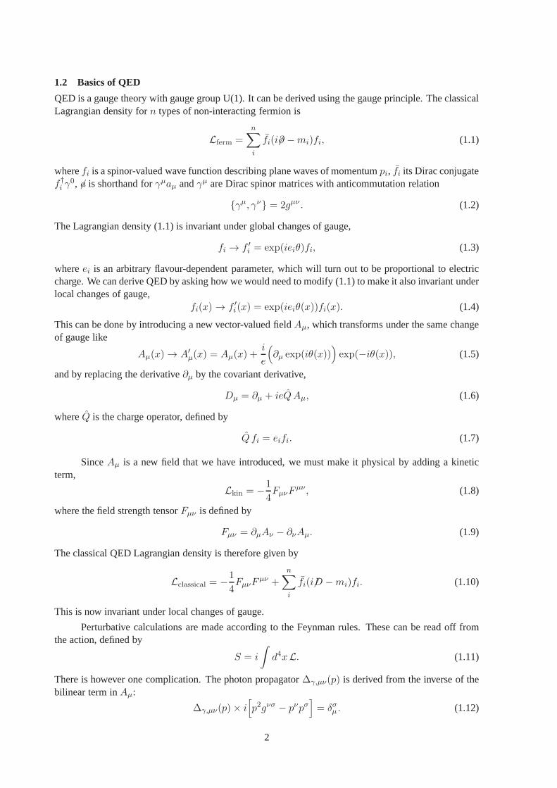
There is however one complication. The photon propagator∆γ,µν(p) is derived from the inverse of thebilinear term inAµ:
∆γ,µν(p)× i[
p2gνσ − pνpσ]
= δσµ . (1.12)
2
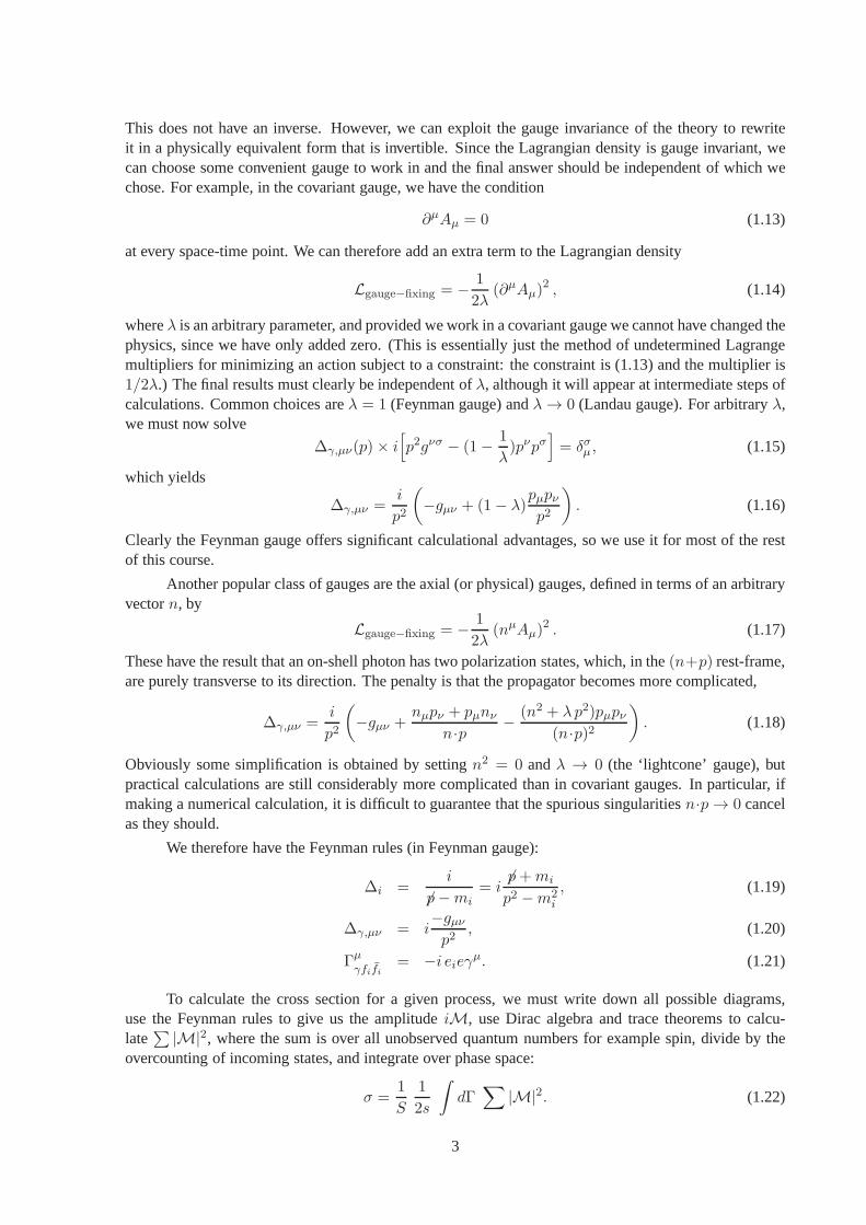
This does not have an inverse. However, we can exploit the gauge invariance of the theory to rewriteit in a physically equivalent form that is invertible. Sincethe Lagrangian density is gauge invariant, wecan choose some convenient gauge to work in and the final answer should be independent of which wechose. For example, in the covariant gauge, we have the condition
∂µAµ = 0 (1.13)
at every space-time point. We can therefore add an extra termto the Lagrangian density
Lgauge−fixing = − 1
2λ(∂µAµ)
2 , (1.14)
whereλ is an arbitrary parameter, and provided we work in a covariant gauge we cannot have changed thephysics, since we have only added zero. (This is essentiallyjust the method of undetermined Lagrangemultipliers for minimizing an action subject to a constraint: the constraint is (1.13) and the multiplier is1/2λ.) The final results must clearly be independent ofλ, although it will appear at intermediate steps ofcalculations. Common choices areλ = 1 (Feynman gauge) andλ→ 0 (Landau gauge). For arbitraryλ,we must now solve
∆γ,µν(p)× i[
p2gνσ − (1− 1
λ)pνpσ
]
= δσµ , (1.15)
which yields
∆γ,µν =i
p2
(
−gµν + (1− λ)pµpνp2
)
. (1.16)
Clearly the Feynman gauge offers significant calculationaladvantages, so we use it for most of the restof this course.
Another popular class of gauges are the axial (or physical) gauges, defined in terms of an arbitraryvectorn, by
Lgauge−fixing = − 1
2λ(nµAµ)
2 . (1.17)
These have the result that an on-shell photon has two polarization states, which, in the(n+p) rest-frame,are purely transverse to its direction. The penalty is that the propagator becomes more complicated,
∆γ,µν =i
p2
(
−gµν +nµpν + pµnν
n·p − (n2 + λ p2)pµpν(n·p)2
)
. (1.18)
Obviously some simplification is obtained by settingn2 = 0 andλ → 0 (the ‘lightcone’ gauge), butpractical calculations are still considerably more complicated than in covariant gauges. In particular, ifmaking a numerical calculation, it is difficult to guaranteethat the spurious singularitiesn·p→ 0 cancelas they should.
We therefore have the Feynman rules (in Feynman gauge):
∆i =i
6p−mi= i
6p+mi
p2 −m2i
, (1.19)
∆γ,µν = i−gµνp2
, (1.20)
Γµγfifi
= −i eieγµ. (1.21)
To calculate the cross section for a given process, we must write down all possible diagrams,use the Feynman rules to give us the amplitudeiM, use Dirac algebra and trace theorems to calcu-late
∑ |M|2, where the sum is over all unobserved quantum numbers for example spin, divide by theovercounting of incoming states, and integrate over phase space:
σ =1
S
1
2s
∫
dΓ∑
|M|2. (1.22)
3
An element ofn-body phase space is given by
dΓ =n∏
i=1
(
d4pi(2π)4
(2π)δ(p2i −m2i )
)
(2π)4δ4(ptot −∑n
i pi) (1.23)
=
n∏
i=1
(
d3pi(2π)32Ei
)
(2π)4δ4(ptot −∑n
i pi). (1.24)
For example, the cross section fore+e− → µ+µ− is calculated as follows. The amplitude is
iM = v(pe+)(ie)γµu(pe−) i
−gµν(pe+ + pe−)
2u(pµ−)(ie)γνv(pµ+) (1.25)
=−ie2
(pe+ + pe−)2v(pe+)γ
µu(pe−) u(pµ−)γµv(pµ+) (1.26)
and hence∑
|M|2 =(4πα)2
s2Tr 6pe+γµ6pe−γν Tr
6pµ−γµ6pµ+γν
, (1.27)
whereα = e2/4π ands = (pe+ + pe−)2, or
∑
|M|2 =16(4πα)2
s2(
pµe+pνe− + pµ
e−pνe+ − pe+ ·pe−gµν
) (
pµ−,µpµ+,ν + pµ+,µpµ−,ν − pµ+ ·pµ−gµν)
(1.28)
= 8(4πα)2t2 + u2
s2, (1.29)
wheret = (pe− − pµ−)2 andu = (pe− − pµ+)2 = −s− t. The cross section is therefore
σ =1
4
1
2s
∫ 0
−s
dt
8πs8(4πα)2
t2 + u2
s2(1.30)
=4πα2
3s. (1.31)
1.3 SU(3) and colour
QCD can be derived in exactly the same way as QED: we start fromthe Lagrangian density for a setof non-interacting quarks and modify it in just such a way that it is invariant under changes of gauge.The only difference is that instead of the gauge transformation being a simple phase (U(1) group), weconsider a non-Abelian group SU(Nc). This has several important consequences. Fermion charges willcome inNc different types, called colours, they will be quantized (incontrast to the electric chargesei,which could take any value) and, most importantly, the gaugebosons will be self-interacting.
It has been well-known since the early days of QCD that there are three colours, for examplefrom baryon wave functions, the totale+e− cross section (which is proportional toNc) andπ0 decayrate (which is proportional toN2
c ). However, in most calculations it is useful to keep the number ofcoloursNc arbitrary until the very last step when it is set equal to three. TheNc-dependent coefficientsare a useful diagnostic tool in understanding the physical origins of different terms, comparing differentcalculations and tracking down errors.
We start by restating briefly some features of SU(N ), the group ofN×N unitary matrices (U †U =1) with determinant +1. LetU be an element of SU(N ) that is infinitesimally close to the identity andwrite it as
U = 1 + iG, (1.32)
4
whereG has infinitesimal entries. It must be hermitian (G† = G) and traceless. One can choose a basisset ofN2 − 1 matrices,tA, A = 1, . . . , N2 − 1, such that anyG can be written as
G =N2−1∑
A
ǫAtA, (1.33)
whereǫA are infinitesimal numbers. Note that I will always denote colour indices that run from 1 toNby a and from 1 toN2−1 byA. ThetA are called the generators of the group and define its fundamentalrepresentation. You can show that[tA, tB ] is antihermitian and traceless and hence can be written as alinear combination of othertCs,
[tA, tB ] ≡ i fABCtC , (1.34)
wherefABC are a set of real constants, called the structure constants of the group. It is straightfor-ward to see thatfABC is antisymmetric inA,B, and with a little more work, one can prove that it isantisymmetric in all its indices. Equation (1.34) defines the Lie algebra of the group.
We can also define a set of(N2−1)× (N2−1) matrices that obey the same algebra:
(
TA)
BC≡ −ifABC , (1.35)
[TA, TB] = i fABCTC . (1.36)
These define the group’s adjoint representation.
Although we started with elements infinitesimally close to the identity matrix, we can calculate anarbitrary elementU by stringing together an infinite number of infinitesimal elements,
U = limN→∞
(1 + iθAtA/N)N = exp(iθAtA) ≡ exp(it·θ). (1.37)
SinceU is unitary andtA hermitian, we have
U−1 = exp(−it·θ). (1.38)
There are several identities we will require time and time again:
Tr(tAtB) = 12δ
AB ≡ TRδAB (1.39)
∑
A
tAabtAbc =
N2 − 1
2Nδac ≡ CF δac (1.40)
Tr(TCTD) =∑
A,B
fABCfABD = NδCD ≡ CAδCD, (1.41)
where the constantsCF andCA are the Casimir operators of the fundamental and adjoint representationsof the group respectively. Although we know the numerical values of these constants:
TR =1
2, (1.42)
CF =4
3, (1.43)
CA = 3, (1.44)
it is good practice, as I said, to leave them unexpanded in allalgebraic results.
In fact for practical calculations one only requires these,and other similar, identities and never anexplicit representation fortA or fABC .
5
1.4 The QCD Lagrangian
The classical Lagrangian density forn non-interacting quarks with massesmi is
Lquarks =
n∑
i
qai (i6∂ −mi)abqbi , (1.45)
where the factor(i6∂−mi)ab is proportional to the identity matrix in colour space. Thisis invariant underglobal SU(Nc) transformations,
qa → q′a = exp(it·θ)abqb. (1.46)
To make it invariant under local transformations,
qa(x) → q′a(x) = exp(it·θ(x))abqb(x), (1.47)
we have to introduce the covariant derivative,
Dµ,ab = ∂µ 1ab + igs (t·Aµ)ab, (1.48)
whereAAµ are coloured vector fields that transform in just the right way that we have
D′µ,abq
′b(x) = exp(it·θ(x))abDµ,bcqc(x), (1.49)
giving
t·A′µ = exp(it·θ(x)) t·Aµ exp(−it·θ(x)) + i
gs
(
∂µ exp(it·θ(x)))
exp(−it·θ(x)). (1.50)
We again have to introduce a kinetic term for this new field,
Lkin = −1
4FAµνF
µνA , (1.51)
whereFAµν is the non-Abelian field strength tensor. However, the definition we used in QED (1.9) does
not result in an invariant Lagrangian density under transformation (1.50). One must add an extra term,
FAµν = ∂µA
Aν − ∂νA
Aµ − gsf
ABCABµA
Cν , (1.52)
and only then is (1.51) invariant under gauge transformations.
This extra term has profound consequences for the theory: itmeans that gluons are self-interacting,through three- and four-point vertices. This will turn out to give rise to asymptotic freedom at highenergies and strong interactions at low energies, among themost fundamental properties of QCD. Wetherefore see that these are absolute requirements of the SU(Nc) gauge symmetry.
Before reading off the Feynman rules we again have to fix the gauge. This proceeds in exactly thesame way as in QED, leading to, in covariant gauges,
Lgauge−fixing = − 1
2λ
(
∂µAAµ
)2. (1.53)
Finally, it turns out that in a non-Abelian gauge theory, it is necessary to add one extra termto the Lagrangian density, related to the need for ghost particles. These are beyond the scope of thiscourse, but basically they arise because when a non-Abeliangauge theory is renormalized it is possiblefor unphysical degrees of freedom to propagate freely. These are cancelled off by introducing into thetheory an unphysical set of fields, the ghosts, which are scalars but have Fermi statistics. For practicalpurposes it is enough to know that there exist Feynman rules for ghosts and that in every diagram witha closed loop of internal gluons containing only triple-gluon vertices, we must add a diagram with thegluons in the loop replaced by ghosts. It is worth noting thatin physical gauges, as the name suggests,ghost contributions always vanish and they can be ignored.
The final Lagrangian is therefore
LQCD = −1
4FAµνF
µνA +
n∑
i
qai (i6D −mi)abqbi −
1
2λ
(
∂µAAµ
)2+ Lghost. (1.54)
6
1.5 Feynman rules
Just as in QED it is straightforward to read off the Feynman rules from the action. We obtain in Feynmangauge (only the gluon propagator is gauge dependent)
∆abi = δab
i
6p−mi= δabi
6p+mi
p2 −m2i
, (1.55)
∆ABg,µν = δABi
−gµνp2
, (1.56)
Γµgqq = −i gs tA γµ, (1.57)
Γggg = −gsfABC[
(p− q)λgµν + (q − r)µgνλ + (r − p)νgλµ]
. (1.58)
Note that, apart from the triple-gluon vertex, the only difference relative to QED is in the colour struc-ture: propagators are diagonal in colour and the vertex for agluon of colourA to scatter a quark ofcolour b to a quark of colourc contains(tA)cb. Note also that unlike QED the quark–gluon vertex isflavour-independent (it is straightforward to check that, unlike in QED, we cannot introduce a flavour-dependence into the gauge transformation, Eq. (1.47) and retain gauge invariance). In the triple-gluonvertex, the three gluons have momentap, q, r, Lorentz indicesµ, ν, λ and colour indicesA,B,C respec-tively. The momenta are all ingoing:p+ q + r = 0.
The Feynman rules for ghosts and for the four-gluon vertex can be found in ESW [1] (p. 10). Theywill not be needed for this course.
Note also that in analogy with QED the strong chargegs is usually substituted byαS,
αS ≡g2s4π. (1.59)
1.6 e+e−
→ qq
One of the most fundamental quantities in QCD is the totale+e− annihilation cross section to hadrons.We will see in a later lecture that to leading order inαS this is equal to the totale+e− → qq crosssection. The calculation is very similar to that fore+e− → µ+µ−, the only difference being in thecolour structure. The photon is colour blind, so the Feynmanrule for a photon to couple to a quarkcontains a trivial colour matrix,δab. Summing over colours and dividing by the number of incomingcolour states (1 in this case since electrons are not coloured), we therefore obtain
σ(e+e− → qq) = σ(e+e− → µ+µ−)× e2q ×∑
a,b
δabδba. (1.60)
We obtain∑
a,b
δabδba =∑
a
δaa = Nc, (1.61)
and hence
Rhad ≡ σ(e+e− → hadrons)σ(e+e− → µ+µ−)
=∑
q
e2qNc. (1.62)
1.7 e+e−
→ qqg
This process will be important for the higher order corrections toσ(e+e− → hadrons) and particularlyfor the study of three-jet final states ine+e− annihilation, among the most important test-beds for QCD.
There are two Feynman diagrams, shown in Fig. 1.1. We label the momenta and colourse−(p−)+
7
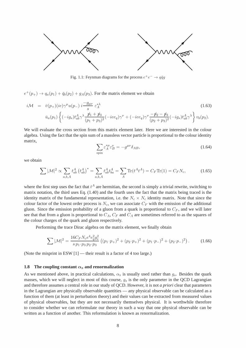
Fig. 1.1: Feynman diagrams for the processe+e− → qqg
e+(p+) → qa(p1) + qb(p2) + gA(p3). For the matrix element we obtain
iM = v(p+)(ie)γµu(p−) i
−gµνs
ε∗λA (1.63)
ua(p1)
(−igs)tAabγλ6p1 + 6p3(p1 + p3)2
(−ieeq)γν + (−ieeq)γν−6p2 − 6p3(p2 + p3)2
(−igs)tAabγλ
vb(p2).
We will evaluate the cross section from this matrix element later. Here we are interested in the colouralgebra. Using the fact that the spin sum of a massless vectorparticle is proportional to the colour identitymatrix,
∑
spin
ε∗µA ενB = −gµνδAB, (1.64)
we obtain
∑
|M|2 ∝∑
a,b,A
tAab(
tAab)∗
=∑
a,b,A
tAabtAba =
∑
A
Tr(tAtA) = CFTr(1) = CFNc, (1.65)
where the first step uses the fact thattA are hermitian, the second is simply a trivial rewrite, switching tomatrix notation, the third uses Eq. (1.40) and the fourth uses the fact that the matrix being traced is theidentity matrix of the fundamental representation, i.e. theNc × Nc identity matrix. Note that since thecolour factor of the lowest order process isNc, we can associateCF with the emission of the additionalgluon. Since the emission probability of a gluon from a quarkis proportional toCF , and we will latersee that that from a gluon is proportional toCA, CF andCA are sometimes referred to as the squares ofthe colour charges of the quark and gluon respectively.
Performing the trace Dirac algebra on the matrix element, wefinally obtain
∑
|M|2 =16CFNce
4e2qg2s
s p1 ·p3 p2 ·p3(
(p1 ·p+)2 + (p2 ·p+)2 + (p1 ·p−)2 + (p2 ·p−)2)
. (1.66)
(Note the misprint in ESW [1] — their result is a factor of 4 toolarge.)
1.8 The coupling constantαS and renormalization
As we mentioned above, in practical calculations,αS is usually used rather thangs. Besides the quarkmasses, which we will neglect in most of this course,gs is the only parameter in the QCD Lagrangianand therefore assumes a central role in our study of QCD. However, it is nota priori clear that parametersin the Lagrangian are physically observable quantities — any physical observable can be calculated as afunction of them (at least in perturbation theory) and theirvalues can be extracted from measured valuesof physical observables, but they are not necessarily themselves physical. It is worthwhile thereforeto consider whether we can reformulate our theory in such a way that one physical observable can bewritten as a function of another. This reformulation is known as renormalization.
8
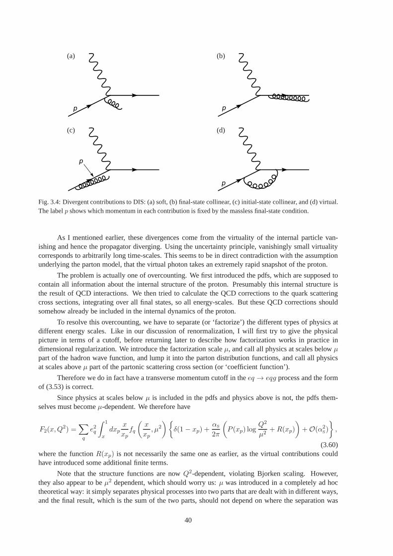
(a) (b) (c) (d)
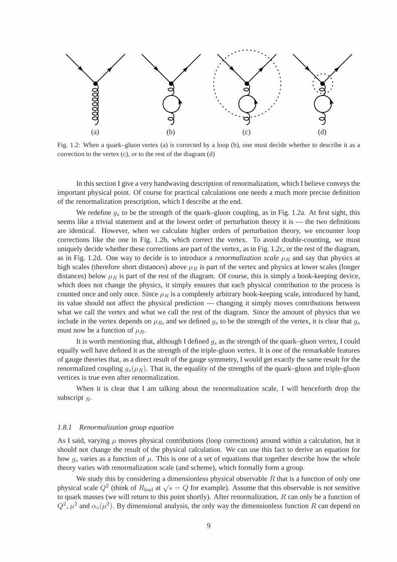
Fig. 1.2: When a quark–gluon vertex (a) is corrected by a loop(b), one must decide whether to describe it as acorrection to the vertex (c), or to the rest of the diagram (d)
In this section I give a very handwaving description of renormalization, which I believe conveys theimportant physical point. Of course for practical calculations one needs a much more precise definitionof the renormalization prescription, which I describe at the end.
We redefinegs to be the strength of the quark–gluon coupling, as in Fig. 1.2a. At first sight, thisseems like a trivial statement and at the lowest order of perturbation theory it is — the two definitionsare identical. However, when we calculate higher orders of perturbation theory, we encounter loopcorrections like the one in Fig. 1.2b, which correct the vertex. To avoid double-counting, we mustuniquely decide whether these corrections are part of the vertex, as in Fig. 1.2c, or the rest of the diagram,as in Fig. 1.2d. One way to decide is to introduce arenormalization scaleµR and say that physics athigh scales (therefore short distances) aboveµR is part of the vertex and physics at lower scales (longerdistances) belowµR is part of the rest of the diagram. Of course, this is simply a book-keeping device,which does not change the physics, it simply ensures that each physical contribution to the process iscounted once and only once. SinceµR is a completely arbitrary book-keeping scale, introduced by hand,its value should not affect the physical prediction — changing it simply moves contributions betweenwhat we call the vertex and what we call the rest of the diagram. Since the amount of physics that weinclude in the vertex depends onµR, and we definedgs to be the strength of the vertex, it is clear thatgsmust now be a function ofµR.
It is worth mentioning that, although I definedgs as the strength of the quark–gluon vertex, I couldequally well have defined it as the strength of the triple-gluon vertex. It is one of the remarkable featuresof gauge theories that, as a direct result of the gauge symmetry, I would get exactly the same result for therenormalized couplinggs(µR). That is, the equality of the strengths of the quark–gluon and triple-gluonvertices is true even after renormalization.
When it is clear that I am talking about the renormalization scale, I will henceforth drop thesubscriptR.
1.8.1 Renormalization group equation
As I said, varyingµ moves physical contributions (loop corrections) around within a calculation, but itshould not change the result of the physical calculation. Wecan use this fact to derive an equation forhow gs varies as a function ofµ. This is one of a set of equations that together describe how the wholetheory varies with renormalization scale (and scheme), which formally form a group.
We study this by considering a dimensionless physical observableR that is a function of only onephysical scaleQ2 (think ofRhad at
√s = Q for example). Assume that this observable is not sensitive
to quark masses (we will return to this point shortly). Afterrenormalization,R can only be a function ofQ2, µ2 andαS(µ
2). By dimensional analysis, the only way the dimensionless functionR can depend on
9
the dimensionful variablesQ2 andµ2 is through their ratio. We can therefore write
R = R(Q2/µ2, αS(µ2)). (1.67)
We can use the fact thatR, as a physical quantity, must be independent of the value ofµ, and the chainrule for partial derivatives, to write
µ2d
dµ2R(Q2/µ2, αS) = 0 =
[
µ2∂
∂µ2+ µ2
∂αS
∂µ2∂
∂αS
]
R (1.68)
≡[
µ2∂
∂µ2+ β(αS)
∂
∂αS
]
R , (1.69)
i.e.,β(αS) ≡ µ2 ∂αS∂µ2 . There are several points to note about this.
– A physical solution is provided byR(1, αS(Q)), i.e., by setting the renormalization scale equal tothe physical scale in the problem.
– Q-dependence of the physical quantityR comes about only because of the renormalization of thetheory and would not be present in the classical theory. Thusmeasuring theQ-dependence ofRdirectly probes the quantum structure of the theory.
– By rearranging Eq. (1.69), one can derive theµ2 dependence ofαS from a calculation ofR,
β(αS) = −µ2 ∂R
∂µ2
∂R∂αS
. (1.70)
– If αS is small,R is perturbatively calculable and henceβ(αS) is too.
Theβ function of QCD is now known to four-loop accuracy,
β(αS) = −α2S(β0 + β1αS + β2α
2S + β3α
2S + . . .). (1.71)
Although the higher orders are essential for quantitative calculation, they are not for qualitative under-standing: almost all QCD phenomenology can be understood using the one loop result,
β0 =11CA − 4TRNf
12π, (1.72)
whereNf is the number of quark flavours that can appear in loops, to be discussed further shortly.
Note thatβ0 is positive and hence that theβ function is negative, at least whenαS is small.This results in asymptotic freedom: the fact that the interactions become weak at high energies (shortdistances) and infrared slavery: the fact that they become strong at low energy.
If we neglect the higher orders, we can solve the renormalization group equation exactly, to obtainαS at some scaleQ as a function of its value at the renormalization scaleµ,
αs(Q2) =
αs(µ2)
1 + αs(µ2)β0 lnQ2
µ2
. (1.73)
1.8.2 Choosingµ2
Although physical quantities do not depend onµ, a calculation truncated at a finite order of perturbationtheory does. We must therefore choose some value forµ. To illustrate this, suppose that our dimension-less physical quantityR has a perturbative expansion that starts atO(αS),
R = R1αS + . . . , (1.74)
10
Fig. 1.3: A measurement ofαS at any scaleQ fixes which curve our universe lies on, but to compare measurementsat different scales we have to agree to label the curves in a standard way, for example usingαS(Mz)
then if we truncate at leading order,
R ≈ R1αS, (1.75)
our truncated expression forR(1, αS(Q)) can be expanded as a power series inαS(µ2)
R(1, αS(Q2)) ≈ R1αS(Q
2) (1.76)
= R1αS(µ2)
[
1− β0αS(µ2) ln
Q2
µ2+ β20α
2S(µ
2) ln2Q2
µ2+ . . .
]
. (1.77)
The leading order result in renormalized perturbation theory is the first term of this series, i.e.,R1αS(µ2).
It is therefore clear that althoughµ is completely arbitrary, choosing it far fromQ guarantees a largetruncation error (note that the converse is not true). One should therefore chooseµ2 ‘close’ toQ2, buthow close is close?
The conventional approach is to setµ = Q and to use theµ variation in a reasonable range, e.g.,Q/2 to 2Q as an estimate of the truncation uncertainty. It should be clear from the foregoing discussionthat this is an extremely arbitrary procedure. However, thefolklore is that in almost all cases wherehigher order corrections have been calculated, they have fallen within the band given by this procedure.
1.8.3 MeasuringαS
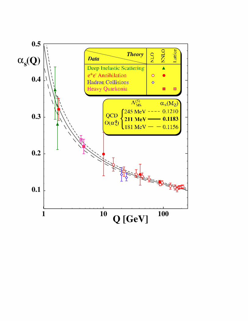
Theβ function tells us howαS varies with scale, but it does not tell us the value ofαS at any particularscale: we need an experimental measurement to do that. Effectively β(αS) defines a family of curves,as illustrated in Fig. 1.3, and one measurement at any scale is sufficient to tell us which curve ouruniverse lies on. However, in order to compare and combine measurements ofαS at different scales,we have to agree on some convenient labeling of the curves. The measurement at any given scale canthen be converted into a measurement of the label. Historically, this was often done using the ‘QCDscale’,ΛQCD, described in the next section, but more recently it has beenrealized that the value ofαS at some fixed scale at which it is relatively small is a lot moreconvenient. Since some of the bestmeasurements come fromZ0 decays, it has become universal to useαS(Mz) as the label. We will discussthe measurements ofαS further in Section 3.1.4.
11
1.8.4 The ‘QCD Scale’,Λ
As I just mentioned, this is another way to label the running coupling, which is to construct a renormal-ization group invariant scale fromαS(µ). Although the Lagrangian of massless QCD has no scale, therenormalization process introduces a dimensionful parameter,
Λ2 = µ2 exp−∫ αS(µ
2) dx
β(x)≈ µ2e−1/β0αS(µ
2), (1.78)
where the approximation uses only the one-loop term in theβ function1.1. This process by which ascaleless theory gets a physically observable scale by the introduction of the unphysical renormalizationscale is known as dimensional transmutation.
At leading order,Λ has a simple interpretation, it is the scale at which the coupling becomesinfinite. However, this interpretation is not self-consistent, since it relies on a truncation of the pertur-bation series in a region in which the coupling is large, ultimately divergent. More generally,Λ can beviewed as a renormalization group invariant parameterization of the scale at which the theory becomesnon-perturbative. All non-perturbative quantities, for example the hadron masses, would be expected tobe of orderΛ.
However,Λ is not a very practically useful label for the value ofαS. This is because its precisevalue, for a given measured value ofαS, depends strongly on the theoretical input used in the calculation,for example which order of perturbation theory we truncateβ at, which renormalization scheme we use,the number of flavours we assume, the way we match the running coupling at the flavour thresholds, etc.
In principle any labeling suffers from these problems, but by using the value ofαS in a regionwhere it is small, and where the scale is not too different from that at which the measurements are made,the impact onαS(Mz) is small, whereasΛ is related to the region whereαS is large, far away from wherethe measurements are made, and these effects are large.
1.8.5 Renormalization in practice
To give a simple physical picture of renormalization, I havedescribed it in terms of a cutoff on the scaleof the physical effects that are included in different components of a Feynman diagram calculation. How-ever, in practice, this definition is extremely unattractive, because it breaks Lorentz and gauge invariance,two of the fundamental symmetries of our theory. If calculating in this scheme, these symmetries willget violated by a truncation at any finite order of perturbation theory and only restored in an all orderscalculation. There are other simple schemes that work well in certain cases, for example the Pauli–Villarsregularization, but the only known scheme consistent with all the symmetries of QCD, and hence guar-anteed to work at any order of perturbation theory, isdimensional regularization. In this section I give avery brief description of how this works in practice. The difference betweenµ andµR will be (slightly)relevant here, so I temporarily reinstate the subscript.
The basic observation is that the loop corrections that we have been discussing are divergent infour or more space-time dimensions, but are finite in less than four dimensions. We therefore chooseto calculate our Feynman diagrams ind < 4 dimensions (we always work in Minkowski space, withone time dimension andd−1 space dimensions). With a little thought, we can analytically continue
1.1Note that the definition in the first equality of Eq. (1.78), while formally renormalization group invariant, is not prac-tically useful, since the lower limit of the integration is not defined (corresponding to the fact that any definition ofΛ thatdiffers by a multiplicative constant is equally renormalization group invariant). For perturbative calculations, various def-initions, equivalent to Eq. (1.78) to the order to which theyare defined, can be used. For non-perturbative calculations,for example in lattice QCD, the precise definition is more critical. A commonly-used convention (see for example [3]) is
Λ2 = µ2 exp
−
1β0αS(µ
2)−
β1
β20
logαS(µ2)−
∫ αS(µ2)
0dx
(
1β(x)
+1−
β1β0
x
β0x2
)
. In contrast to the definition given in [1], for
example, this can be seen to depend only on theβ function atαS(µ2) and at smaller values, so is well-defined perturbatively
and, as can be easily checked, is exactly renormalization scheme invariant.
12
the number of dimensions to be a complex number such that at the end of the calculation, after therenormalization prescription has been followed, we can letit smoothly tend back to 4 and obtain finiteresults. We therefore defined = 4− 2ǫ and consider theǫ→ 0+ limit.
By counting the dimensionality of terms in the Lagrangian, we discover that the coupling constantbecomes dimensionful ind 6= 4 dimensions. This is not very convenient, so we define a dimensionlessparameterαS, by introducing a completely arbitrary scaleµ,
α(d)S = αS µ
2ǫ, (1.79)
whereα(d)S is the dimensionfuld-dimensional coupling.µ is called the regularization scale. It is often set
equal to the renormalization scaleµR, but I consider this confusing since we have not yet renormalizedthe theory, so, for now, I keep them distinct and only set themequal again at the end of this section.
When calculating loop corrections, we then find terms that have 1/ǫ singularities for smallǫ.These have the right form to be absorbed by a redefinition (i.e. a renormalization) of the coupling. Sincewe also want the renormalized coupling to be dimensionless,we have to introduce a dimensionful scaleat which the renormalization is performed,µR. To make this concrete, at one-loop order, the prescriptionis straightforward: after calculating all the one-loop diagrams, rewrite all occurrences ofαS in terms ofthe renormalized coupling,
αS(µR) = αS + β0 F (ǫ)
(
µ2
µ2R
)ǫ1
ǫα2
S . (1.80)
ProvidedF (0) = 1, once this substitution has been made, the amplitude is finite. That is, theǫ polesthat this expression produces exactly cancel those from theone-loop calculation. Moreover, the arbitraryscaleµ cancels from the amplitude at this point. One is left with a finite amplitude that depends only onµR andαS(µR), in exactly the same way as discussed earlier.
The arbitrary functionF (ǫ) = 1 + O(ǫ) defines the renormalization scheme. More precisely, itdefines what finite parts of the loop amplitude are subtractedinto the renormalized coupling, in additionto the divergent part. The MS, or minimal subtraction, scheme, is defined by subtracting nothing else,
FMS(ǫ) = 1. (1.81)
The most commonly used scheme is theMS, or modified minimal subtraction, scheme, in which oneidentifies some additional overall factors coming from the analytical continuation of the angular inte-grations in the one-loop calculation. Since they are universal it is convenient to subtract them into thecoupling,
FMS(ǫ) =(4π)ǫ
Γ(1− ǫ)= 1 + (ln 4π − γE)ǫ, (1.82)
whereΓ is the Euler gamma function andγE the Euler gamma constant,γE ≈ 0.577216. Note that thetwo expressions on the right-hand side of Eq. (1.82) differ at orderǫ2. Different practitioners use eitherof the two definitions, resulting in a finite difference at twoloops that is straightforward to keep track of.
1.9 Quark masses and decoupling
The quark massesmq are also parameters of the Lagrangian and face the same issues: for a physicalcalculation we should redefine them in a physical way. For theelectron mass, we have a simple definition:we can isolate a single electron and ‘weigh’ it in the laboratory. That is, we can define its mass throughthe classical limit. We cannot use the same procedure for quarks, because confinement means that wecan never take a single quark off to our laboratory to weigh itindividually. We must therefore definesome other renormalization procedure.
13
It is possible to proceed in close analogy with the coupling strength. We renormalize our the-ory at the same scaleµ. We encounter gluon loop corrections to the quark propagator and absorbthe part of them at scales aboveµ into the definition of the mass. We therefore obtain a ‘running’(i.e. scale-dependent) mass. Just like for the coupling, wecan obtain a renormalization group equationwith perturbatively-calculable coefficients,
µ2
m
dm
dµ2= − 1
παS(µ
2) + . . . . (1.83)
At leading order it can be solved exactly, to give
m(µ2) =M[
αS(µ2)]
1πβ0 , (1.84)
whereM is a renormalization group invariant constant (c.f.ΛQCD). Note that increasingµ2 decreasesm2.Thus quarks appear to get lighter as they are probed at scalesfurther and further above their masses.
An alternative scheme, which is often used in electroweak physics, and in the physics of heavymesons, is thepole mass. Here one definesmq to be the pole of the propagatori( 6 p +mq)/(p
2 −m2q)
to all orders. This is very useful forQ ∼ mq, but it turns out that it is similar to a running mass schemewith µ of ordermq and hence generates large logarithms and a large truncationerror forQ≫ mq.
If our dimensionless observableR is finite for massless quarks then the quark mass effects mustvanish smoothly as the mass goes to zero. Therefore the mass effects must be suppressed by(mq/Q)n,with n ≥ 1. If there are quarks with mass much greater thanQ, they can only affect our observablethrough loop corrections. A dimensional argument shows that such corrections must be suppressed by(Q/mq)
n, with n ≥ 2.
These observations form the basis of the decoupling theorem, in which quarks heavier than ourphysical scale can be ignored, and quarks lighter than it canbe treated as massless. Thus, for most QCDcalculations, we work withNf flavours of massless quark (recall theNf that appeared inβ0). Care mustbe taken whenQ is close to a quark mass, or we study a range of processes at scales that span a quarkmass, but in fact for most of the phenomenology considered inthis course we can simply takeNf to befixed,Nf = 5.
1.10 Summary
We have seen that QCD is a gauge theory. The fact that the gaugesymmetry is non-Abelian predicts thatthe gluon is self-interacting. This leads to the fact that the theory becomes strongly interacting at lowenergies, and hence non-perturbative, and weakly interacting at high energies so that perturbation theorycan be used.
The main tools that we will use to study QCD are thefactorizationof non-perturbative effects andthe renormalizationanddecouplingof high-energy physics. These allow us to use perturbation theoryand, in particular, the Feynman rules, to study the phenomenology of QCD.
2 QCD PHENOMENOLOGY AT TREE LEVEL
Leading order perturbation theory, together with the one-loop renormalization group equation is enoughto understand a wide variety of QCD phenomenology. In this section, we briefly review the phenomenol-ogy of QCD before introducing the complications of loop corrections to it in the following section. Mostof the salient ideas are introduced in the context ofe+e− annihilation and deep inelastic scattering, butapply equally well to hadron collisions and photoproduction, which we discuss more briefly at the end.
2.1 The cross section fore+e−
→ hadrons
One of the most striking features ofe+e− annihilation events is the fact that many of them produce manyhadrons. In trying to calculate the cross section for this process, however, we are immediately faced with
14
a problem: the Lagrangian does not contain any information about hadrons, so there are no Feynmanrules involving them. Even if there were, calculating all the diagrams for events involving thirty or fortyparticles would be prohibitively complicated, let alone integrating them over the corresponding phasespace to produce a total cross section. Fortunately a simpleapplication of the Feynman rules of QED,together with some simple symmetry arguments, allows us to make a surprisingly strong statement aboutthe cross section fore+e− annihilation to hadrons.
We postulate that the matrix element for the sum of all diagrams in which a virtual photon withLorentz indexν and momentumq produces a particular set ofn hadrons with momentap1 . . . pn isknown and parameterize it by a functionTν(n, q, p1 . . . pn). Using this function, it is straightforwardto write down the matrix element for the full process,
M = v(q2)eγµu(q1)−gµνq2
Tν(n, q, p1 . . . pn) (2.1)
and hence the phase-space integral for its total cross section. The total cross section to produce anynumber of any type of hadrons is then simply given by the sum ofthis integral over hadron type andmultiplicity (both generically represented by
∑
n),
σ =1
2s
1
4
e2
s2Tr(6q2γµ6q1γν) (2.2)
×∑
n
∫
dPSn Tµ(n, q, p1 . . . pn) T ∗ν (n, q, p1 . . . pn). (2.3)
We then define a new two-index tensor,Hµν , to represent this sum of integrals,
Hµν(q) ≡∑
n
∫
dPSn Tµ T∗ν , (2.4)
which after the integration and summation can only be a function of q2.1. Now, there are only twopossible Lorentz covariant two-index tensor functions of one four-vector,gµν andqµqν . We therefore pa-rameterizeHµν as a linear combination of these, with coefficients that are functions of the only availableLorentz scalar,q2,
Hµν = A(q2)gµν +B(q2)qµqν . (2.5)
Finally, since the theory is gauge invariant (in practice boiling down to invariance under the changeεµ → εµ + qµ for the polarization vector of a photon of momentumq), Hµν must be perpendicular tobothqµ andqν ,
qµHµν = qνHµν = 0, (2.6)
giving a relation between the two functions,
A = −q2B. (2.7)
The final step is to realize thatB(s) has to be dimensionless. Since it is a function of only one dimen-sionful parameter, it must therefore be constant. We therefore have the fundamental prediction that (forenergies well above all hadron masses) the cross section to produce any number of hadrons is propor-tional to that to produce a muon–antimuon pair,
R(e+e−) ≡ σ(e+e− → hadrons)σ(e+e− → µ+µ−)
= constant, (2.8)
2.1Can you spot the flaw in this argument? It assumes that all information about the hadron momenta is washed out by theintegration, which is only true if they are massless. In general sincep2h is fixed atm2
h during the integration,H also dependsin a complicated way on the masses of all possible hadrons. Infact we will shortly justify, on the basis of a space-time picture,neglecting these, in the limit thatq2 is much greater than allm2
h. It also ignores any other masses in the problem, like the Zmass, which we remedy later on.
15
Fig. 2.1: Space-time sketch of the production of a hadron ine+e− annihilation
without knowing anything about the interactions of hadrons!
In order to go further than this and try to predict this constant, or learn something from its mea-surement, we need a specific model of the production of hadrons. This is provided by thequark partonmodel. Of course this can be more rigorously derived, but I find it more useful to illustrate the physicswith a space-time argument, see Fig. 2.1. Since the photon ishighly virtual, it is produced and decays toquarks in a small space-time volume,t ∼ 1/
√s. On the other hand, the wavefunction of a hadron with
mass∼ mhad has spatial extent∼ 1/mhad and hence the confinement of a quark pair into the hadrontakest ∼ 1/mhad. Thus there is no time for the confinement to affect the annihilation cross section andwe expect
σ(e+e− → hadrons) ≈ σ(e+e− → quarks), (2.9)
and the Feynman rules do tell us how to calculate that.
In fact, we can go further than that and use an argument from quantum mechanics to postulate theform of the corrections to this approximation. Over a regionof size∼ 1/
√s, the amount by which the
wave function of a hadron with spatial extent∼ 1/mhad, could vary is∼ mhad/√s and the corrections
should be at least this to some positive power,
σ(e+e− → hadrons) = σ(e+e− → quarks)×(
1 +O(
mhad√s
)n)
. (2.10)
On the basis of the space-time picture, we can only justify that the corrections to the quark parton modelare suppressed by some (positive) power of the ratio of scales. In practice,n is believed to be 6 fore+e−
annihilation, making these corrections so small as to be almost impossible to measure. For most crosssections however,n is 2, and for jet cross sections, 1.
We calculated the cross section fore+e− → qq in Section 1.6 and obtained
Re+e− ≡ σ(hadrons)
σ(muons)= Nc
∑
q
e2q, (2.11)
where the sum overq is over all quark flavours that are kinematically allowed, i.e. for which√s > 2mq.
If we ignore effects close to threshold, such as the formation of bound states, we can expect a plot ofRe+e− against
√s to present a series of steps at twice the quark masses and be flat in between. In
principle one can read off the quark masses and charges from this plot.
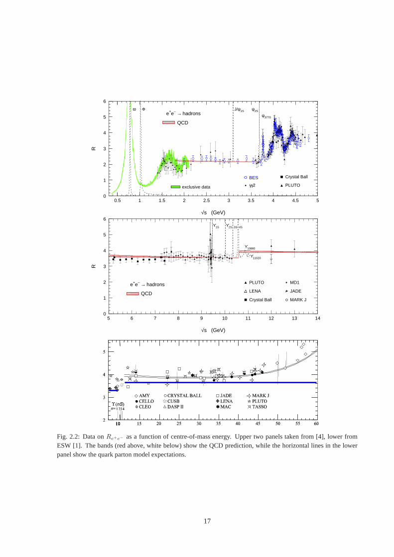
Looking at the data in Fig. 2.2, we see that the general trend is as expected, but there are clearlycorrections that are not accounted for by the quark parton model. One of these is the effect of higher
16
0
1
2
3
4
5
6
0.5 1 1.5 2 2.5 3 3.5 4 4.5 5
exclusive data
e+e– → hadrons
QCD
γγ2
Crystal Ball
PLUTO
BES
ω Φ J/ψ1S ψ2S
ψ3770
√s (GeV)
R
0
1
2
3
4
5
6
5 6 7 8 9 10 11 12 13 14
e+e– → hadrons
QCD
PLUTO
LENA
Crystal Ball
MD1
JADE
MARK J
ϒ1S ϒ2S 3S 4S
ϒ10860
ϒ11020
√s (GeV)
R
Fig. 2.2: Data onRe+e− as a function of centre-of-mass energy. Upper two panels taken from [4], lower fromESW [1]. The bands (red above, white below) show the QCD prediction, while the horizontal lines in the lowerpanel show the quark parton model expectations.
17
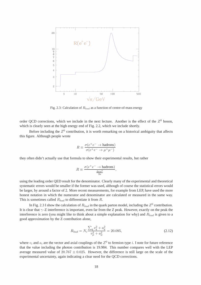
Fig. 2.3: Calculation ofRhad as a function of centre-of-mass energy
order QCD corrections, which we include in the next lecture.Another is the effect of theZ0 boson,which is clearly seen at the high energy end of Fig. 2.2, whichwe include shortly.
Before including theZ0 contribution, it is worth remarking on a historical ambiguity that affectsthis figure. Although people wrote
R ≡ σ(e+e− → hadrons)σ(e+e− → µ+µ−)
they often didn’t actually use that formula to show their experimental results, but rather
R ≡ σ(e+e− → hadrons)4πα2
3s
,
using the leading order QED result for the denominator. Clearly many of the experimental and theoreticalsystematic errors would be smaller if the former was used, although of course the statistical errors wouldbe larger, by around a factor of 2. More recent measurements,for example from LEP, have used the morehonest notation in which the numerator and denominator are calculated or measured in the same way.This is sometimes calledRhad to differentiate it fromR.
In Fig. 2.3 I show the calculation ofRhad in the quark parton model, including theZ0 contribution.It is clear thatγ–Z interference is important, even far from the Z peak. However, exactly on the peak theinterference is zero (you might like to think about a simple explanation for why) andRhad is given to agood approximation by the Z contribution alone,
Rhad = Nc
∑
q v2q + a2q
v2µ + a2µ= 20.095, (2.12)
wherevi andai are the vector and axial couplings of theZ0 to fermion typei. I note for future referencethat the value including the photon contribution is 19.984.This number compares well with the LEPaverage measured value of20.767 ± 0.025. However, the difference is still large on the scale of theexperimental uncertainty, again indicating a clear need for the QCD corrections.
18
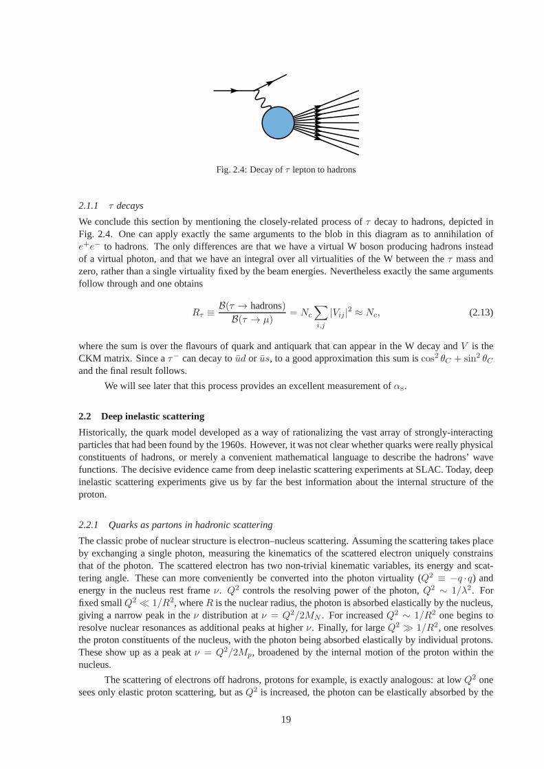
Fig. 2.4: Decay ofτ lepton to hadrons
2.1.1 τ decays
We conclude this section by mentioning the closely-relatedprocess ofτ decay to hadrons, depicted inFig. 2.4. One can apply exactly the same arguments to the blobin this diagram as to annihilation ofe+e− to hadrons. The only differences are that we have a virtual W boson producing hadrons insteadof a virtual photon, and that we have an integral over all virtualities of the W between theτ mass andzero, rather than a single virtuality fixed by the beam energies. Nevertheless exactly the same argumentsfollow through and one obtains
Rτ ≡ B(τ → hadrons)B(τ → µ)
= Nc
∑
i,j
|Vij |2 ≈ Nc, (2.13)
where the sum is over the flavours of quark and antiquark that can appear in the W decay andV is theCKM matrix. Since aτ− can decay toud or us, to a good approximation this sum iscos2 θC + sin2 θCand the final result follows.
We will see later that this process provides an excellent measurement ofαS.
2.2 Deep inelastic scattering
Historically, the quark model developed as a way of rationalizing the vast array of strongly-interactingparticles that had been found by the 1960s. However, it was not clear whether quarks were really physicalconstituents of hadrons, or merely a convenient mathematical language to describe the hadrons’ wavefunctions. The decisive evidence came from deep inelastic scattering experiments at SLAC. Today, deepinelastic scattering experiments give us by far the best information about the internal structure of theproton.
2.2.1 Quarks as partons in hadronic scattering
The classic probe of nuclear structure is electron–nucleusscattering. Assuming the scattering takes placeby exchanging a single photon, measuring the kinematics of the scattered electron uniquely constrainsthat of the photon. The scattered electron has two non-trivial kinematic variables, its energy and scat-tering angle. These can more conveniently be converted intothe photon virtuality (Q2 ≡ −q ·q) andenergy in the nucleus rest frameν. Q2 controls the resolving power of the photon,Q2 ∼ 1/λ2. Forfixed smallQ2 ≪ 1/R2, whereR is the nuclear radius, the photon is absorbed elastically bythe nucleus,giving a narrow peak in theν distribution atν = Q2/2MN . For increasedQ2 ∼ 1/R2 one begins toresolve nuclear resonances as additional peaks at higherν. Finally, for largeQ2 ≫ 1/R2, one resolvesthe proton constituents of the nucleus, with the photon being absorbed elastically by individual protons.These show up as a peak atν = Q2/2Mp, broadened by the internal motion of the proton within thenucleus.
The scattering of electrons off hadrons, protons for example, is exactly analogous: at lowQ2 onesees only elastic proton scattering, but asQ2 is increased, the photon can be elastically absorbed by the
19
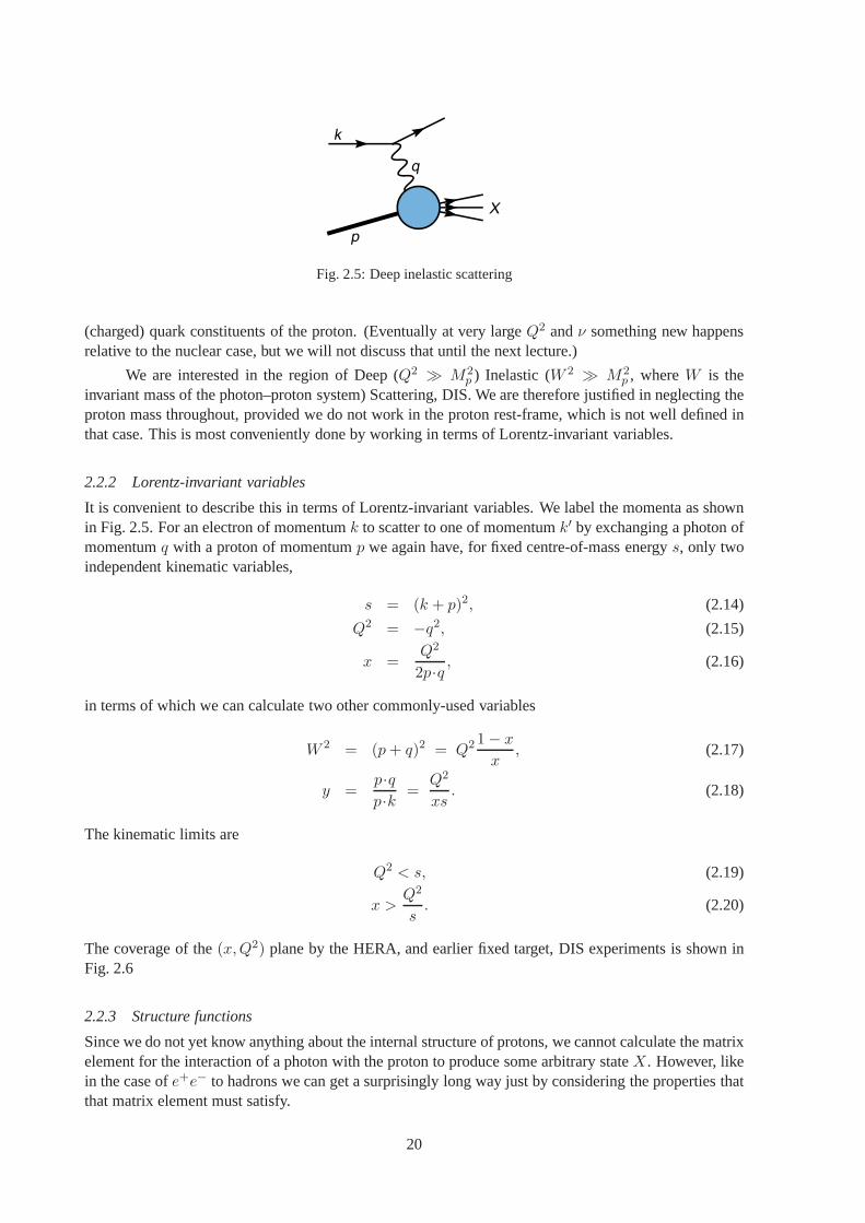
Fig. 2.5: Deep inelastic scattering
(charged) quark constituents of the proton. (Eventually atvery largeQ2 andν something new happensrelative to the nuclear case, but we will not discuss that until the next lecture.)
We are interested in the region of Deep (Q2 ≫ M2p ) Inelastic (W 2 ≫ M2
p , whereW is theinvariant mass of the photon–proton system) Scattering, DIS. We are therefore justified in neglecting theproton mass throughout, provided we do not work in the protonrest-frame, which is not well defined inthat case. This is most conveniently done by working in termsof Lorentz-invariant variables.
2.2.2 Lorentz-invariant variables
It is convenient to describe this in terms of Lorentz-invariant variables. We label the momenta as shownin Fig. 2.5. For an electron of momentumk to scatter to one of momentumk′ by exchanging a photon ofmomentumq with a proton of momentump we again have, for fixed centre-of-mass energys, only twoindependent kinematic variables,
s = (k + p)2, (2.14)
Q2 = −q2, (2.15)
x =Q2
2p·q , (2.16)
in terms of which we can calculate two other commonly-used variables
W 2 = (p+ q)2 = Q2 1− x
x, (2.17)
y =p·qp·k =
Q2
xs. (2.18)
The kinematic limits are
Q2 < s, (2.19)
x >Q2
s. (2.20)
The coverage of the(x,Q2) plane by the HERA, and earlier fixed target, DIS experiments is shown inFig. 2.6
2.2.3 Structure functions
Since we do not yet know anything about the internal structure of protons, we cannot calculate the matrixelement for the interaction of a photon with the proton to produce some arbitrary stateX. However, likein the case ofe+e− to hadrons we can get a surprisingly long way just by considering the properties thatthat matrix element must satisfy.
20
10-1
1
10
10 2
10 3
10 4
10-6
10-5
10-4
10-3
10-2
10-1
1x
Q2 (
GeV
2 )
y HERA =
1
y HERA =
0.0
05
HERA 94-97
ZEUS BPC 1995H1 SVTX 1995
ZEUS SVTX 1995
HERA 1994
HERA 1993
NMC
BCDMS
E665
SLAC
CCFR
Fig. 2.6: Thex–Q2 plane, showing the coverage of measurements by various experiments
We parameterize the matrix element for a proton of momentump to absorb a photon of momentumq and Lorentz indexµ to produce an arbitrary set of hadronsX with fixed momentapX as
e Tµ(p, q; pX). (2.21)
We therefore have the matrix element squared for the whole process
1
4|M|2 = 1
4
e4
Q4Tr
6kγµ6k′γν
Tµ(p, q; pX)T ∗ν (p, q; pX). (2.22)
For convenience we define the Lorentz tensor
Lµν = Tr
6kγµ6k′γν
. (2.23)
If the stateX consists ofn hadrons, then then+1-body phase space for the whole process can befactorized into a part describing the electron kinematics times then-body phase space forX,
dPS =Q2
16π2sx2dQ2 dx dPSX . (2.24)
This is as far as we can go for a specific stateX, but we can get further by integrating over the phasespace ofX and summing over all possible statesX. We define
∑
X
∫
dPSX1
4|M|2 ≡ e4
Q4LµνHµν , (2.25)
21
or∑
X
∫
dPSX Tµ(p, q; pX)T ∗ν (p, q; pX) = Hµν . (2.26)
Since we have summed and integrated out all dependence onX, Hµν can only depend on the vectorspandq. Since the electromagnetic and strong interactions conserve parity, it must be symmetric inµ andν. There are only four possible symmetric two-index tensors that can be constructed from two vectors,so we can parameterize the hadronic tensor as a linear combination of them:
Hµν = −H1gµν +H2pµpνQ2
+H4qµqνQ2
+H5pµqν + qµpν
Q2, (2.27)
where theHs are scalar functions of the only two Lorentz scalars available q·q = −Q2 andp·q = Q2/2x,i.e., ofx andQ2 only (nots). (Note that we neglectp·p =M2
p since we work in the limit|q·q|, p·q ≫ p·p.)If we includeZ0 exchange (or charged current scattering) we can construct one further tensor,
which is antisymmetric inµ and ν, H3 ǫµνλσpλqσ, whereǫµνλσ is the totally antisymmetric Lorentz
tensor.
Contracting withLµν we find thatH4 andH5 cannot contribute to physical cross sections (thinkabout a simple explanation why not) and we have
LµνHµν = 4k ·k′H1 + 4p·k p·k′Q2
H2. (2.28)
Redefining (just a matter of convention)H1 = 4πF1 andH2 = 8πxF2, we obtain the final result for thescattering cross section
d2σ
dx dQ2=
4πα2
xQ4
[
y2xF1(x,Q2) + (1− y)F2(x,Q
2)]
. (2.29)
Without knowing anything about the interactions of hadrons, we have been able to derive thes depen-dence of the scattering cross section for fixedx andQ2 (which enters through they dependence: recally = Q2/xs).
TheFs are called the structure functions of the proton. It is common to see other linear combina-tions of the structure functions,
FT (x,Q2) = 2xF1(x,Q
2), (2.30)
FL(x,Q2) = F2(x,Q
2)− 2xF1(x,Q2), (2.31)
which correspond to scattering of transverse and longitudinally polarized photons respectively. We there-fore have
d2σ
dx dQ2=
2πα2
xQ4
[
(1 + (1− y)2)FT (x,Q2) + 2(1− y)FL(x,Q
2)]
. (2.32)
In fact the most common form you will see this in nowadays is
d2σ
dx dQ2=
2πα2
xQ4
[
(1 + (1− y)2)F2(x,Q2)− y2FL(x,Q
2)]
. (2.33)
For the majority of current data,y2 is small andFL can be neglected: only close to the kinematic limit,or for very precise data, need it be considered.
We have isolated all the non-trivialx andQ2 dependence into the two functionsF2(x,Q2) and
FL(x,Q2), but we still have no idea how those functions behave. If we make the assumption that the
22
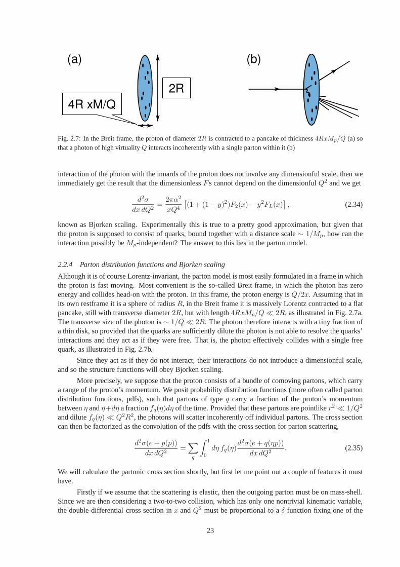
Fig. 2.7: In the Breit frame, the proton of diameter2R is contracted to a pancake of thickness4RxMp/Q (a) sothat a photon of high virtualityQ interacts incoherently with a single parton within it (b)
interaction of the photon with the innards of the proton doesnot involve any dimensionful scale, then weimmediately get the result that the dimensionlessFs cannot depend on the dimensionfulQ2 and we get
d2σ
dx dQ2=
2πα2
xQ4
[
(1 + (1− y)2)F2(x)− y2FL(x)]
, (2.34)
known as Bjorken scaling. Experimentally this is true to a pretty good approximation, but given thatthe proton is supposed to consist of quarks, bound together with a distance scale∼ 1/Mp, how can theinteraction possibly beMp-independent? The answer to this lies in the parton model.
2.2.4 Parton distribution functions and Bjorken scaling
Although it is of course Lorentz-invariant, the parton model is most easily formulated in a frame in whichthe proton is fast moving. Most convenient is the so-called Breit frame, in which the photon has zeroenergy and collides head-on with the proton. In this frame, the proton energy isQ/2x. Assuming that inits own restframe it is a sphere of radiusR, in the Breit frame it is massively Lorentz contracted to a flatpancake, still with transverse diameter2R, but with length4RxMp/Q≪ 2R, as illustrated in Fig. 2.7a.The transverse size of the photon is∼ 1/Q ≪ 2R. The photon therefore interacts with a tiny fraction ofa thin disk, so provided that the quarks are sufficiently dilute the photon is not able to resolve the quarks’interactions and they act as if they were free. That is, the photon effectively collides with a single freequark, as illustrated in Fig. 2.7b.
Since they act as if they do not interact, their interactionsdo not introduce a dimensionful scale,and so the structure functions will obey Bjorken scaling.
More precisely, we suppose that the proton consists of a bundle of comoving partons, which carrya range of the proton’s momentum. We posit probability distribution functions (more often called partondistribution functions, pdfs), such that partons of typeq carry a fraction of the proton’s momentumbetweenη andη+dη a fractionfq(η)dη of the time. Provided that these partons are pointliker2 ≪ 1/Q2
and dilutefq(η) ≪ Q2R2, the photons will scatter incoherently off individual partons. The cross sectioncan then be factorized as the convolution of the pdfs with thecross section for parton scattering,
d2σ(e+ p(p))
dx dQ2=∑
q
∫ 1
0dη fq(η)
d2σ(e+ q(ηp))
dx dQ2. (2.35)
We will calculate the partonic cross section shortly, but first let me point out a couple of features it musthave.
Firstly if we assume that the scattering is elastic, then theoutgoing parton must be on mass-shell.Since we are then considering a two-to-two collision, whichhas only one nontrivial kinematic variable,the double-differential cross section inx andQ2 must be proportional to aδ function fixing one of the
23
variables. Specifically, if we assume that the partons are massless, then we obtain the relation
(q + ηp)2 = 2η p·q −Q2 = 0, (2.36)
orη = x. (2.37)
Secondly if we assume that the struck partons are the quarks of the quark model, they must befermions. Simply from helicity conservation, we can then show thatFL = 0. This is known as theCallan–Gross relation and was one of the first proofs that thequarks of the quark model really were thepartons of the parton model. (If the partons were instead scalars we would haveFT = 0 and hencecompletely differenty-dependence of the cross section.)
2.2.5 Scattering cross sections
To calculate the parton model prediction for the structure functions, we need the matrix elements foreq → eq. These can be obtained by crossing symmetry from those fore+e− → qq. That is,
∑
|M|2 = 8(4πα)2 e2qNc
(pe ·pq)2 + (pe ·p′q)2(pe ·p′e)2
. (2.38)
Converting to the kinematic variables we defined earlier, wehave
∑
|M|2 = 8(4πα)2 e2qNc1 + (1− y)2
y2. (2.39)
Using (2.24), we have
dPS =Q2
16π2sx2dQ2 dx dPSX . (2.40)
SinceX consists only of one massless parton, we have
dPSX =d4pX(2π)3
δ(p2X) (2π)4δ4(ηp + q − pX) (2.41)
= (2π)δ((ηp + q)2) (2.42)
=2πx
Q2δ(η − x). (2.43)
The full cross section is therefore
dσ
dx dQ2=
1
4Nc
1
2s
Q2
16π2sx22πx
Q2δ(x − η)
∑
|M|2 (2.44)
=1
4Nc
y2
16πQ4δ(x − η)
∑
|M|2, (2.45)
where the factor of1/Nc is the average over incoming colours. We therefore have
dσ(e + q)
dx dQ2=
2πα2
Q4δ(x− η) e2q
(
1 + (1− y)2)
(2.46)
and hencedσ(e + p)
dx dQ2=
2πα2
xQ4
(
1 + (1− y)2)
∑
q
e2q xfq(x). (2.47)
Comparing (2.47) with (2.33) we therefore have
F2(x,Q2) =
∑
q
e2q xfq(x), (2.48)
24
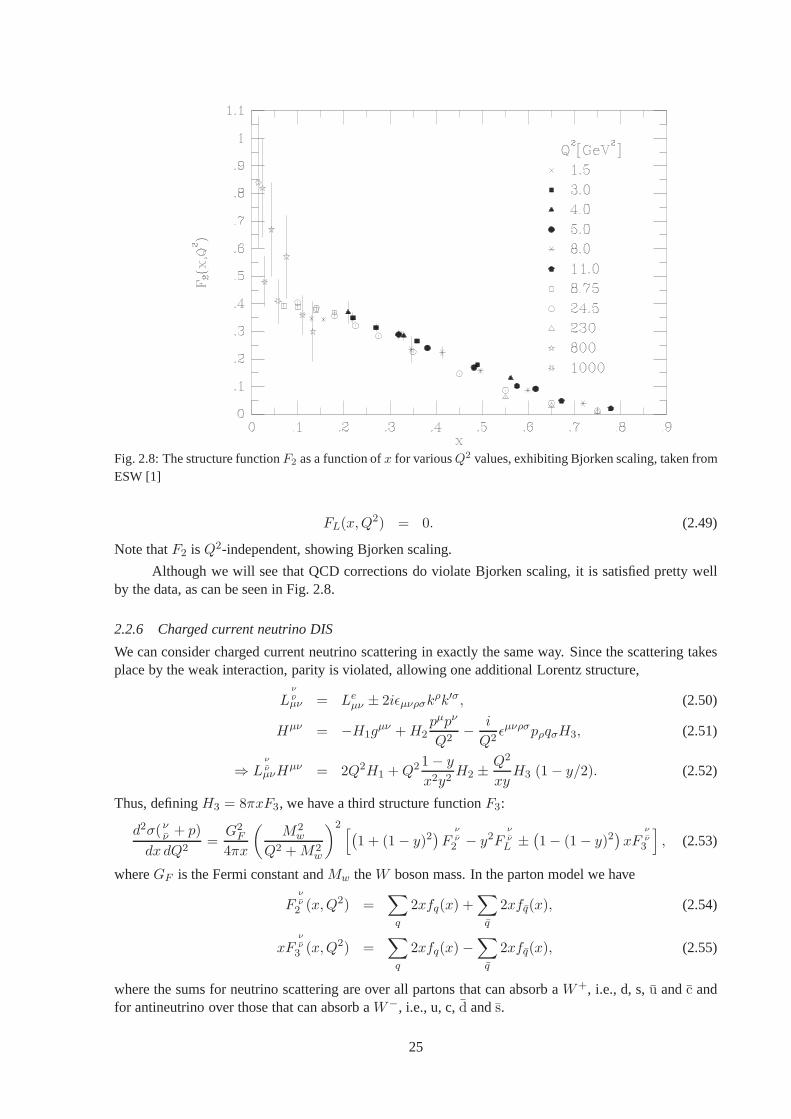
Fig. 2.8: The structure functionF2 as a function ofx for variousQ2 values, exhibiting Bjorken scaling, taken fromESW [1]
Although we will see that QCD corrections do violate Bjorkenscaling, it is satisfied pretty wellby the data, as can be seen in Fig. 2.8.
2.2.6 Charged current neutrino DIS
We can consider charged current neutrino scattering in exactly the same way. Since the scattering takesplace by the weak interaction, parity is violated, allowingone additional Lorentz structure,
Lννµν = Le
µν ± 2iǫµνρσkρk′σ, (2.50)
Hµν = −H1gµν +H2
pµpν
Q2− i
Q2ǫµνρσpρqσH3, (2.51)
⇒ LννµνH
µν = 2Q2H1 +Q2 1− y
x2y2H2 ±
Q2
xyH3 (1− y/2). (2.52)
Thus, definingH3 = 8πxF3, we have a third structure functionF3:
d2σ(νν + p)
dx dQ2=G2
F
4πx
(
M2w
Q2 +M2w
)2[
(
1 + (1− y)2)
Fνν2 − y2F
νν
L ±(
1− (1− y)2)
xFνν3
]
, (2.53)
whereGF is the Fermi constant andMw theW boson mass. In the parton model we have
Fνν2 (x,Q2) =
∑
q
2xfq(x) +∑
q
2xfq(x), (2.54)
xFνν3 (x,Q2) =
∑
q
2xfq(x)−∑
q
2xfq(x), (2.55)
where the sums for neutrino scattering are over all partons that can absorb aW+, i.e., d, s,u andc andfor antineutrino over those that can absorb aW−, i.e., u, c,d ands.
25
Fig. 2.9: Parton distribution function set A from the Martin-Roberts-Stirling group, taken from ESW [1]
2.2.7 Global fits
It is also possible to measure DIS on the neutron, or at least on deuterium from which the neutronstructure functions can be derived. Using strong isospin symmetry, we have the relations
fu/n(x) = fd/p(x), (2.56)
fu/n(x) = fd/p(x), (2.57)
fd/n(x) = fu/p(x), (2.58)
fs/n(x) = fs/p(x), (2.59)
and so on. It is conventional to always refer to the proton case, dropping the “/p” subscript. We thereforehave the slightly confusing result forF en
2 shown below, in whichfd is multiplied by(2/3)2, and so on.
We therefore have
F ep2 = 1
9xfd +49xfu +
19xfd +
49xfu +
19xfs +
19xfs +
49xfc +
49xfc, (2.60)
F en2 = 4
9xfd +19xfu +
49xfd +
19xfu +
19xfs +
19xfs +
49xfc +
49xfc, (2.61)
F νp2 = 2xfd + 2xfu + 2xfs + 2xfc, (2.62)
xF νp3 = 2xfd − 2xfu + 2xfs − 2xfc, (2.63)
F νp2 = 2xfu + 2xfd + 2xfc + 2xfs, (2.64)
xF νp3 = 2xfu − 2xfd + 2xfc − 2xfs. (2.65)
If we make the assumption thatfs = fs andfc = fc, then we have six unknowns for six pieces of dataso, given precise enough data, we could solve for all the pdfsexactly. In practice of course it is never sosimple and one must make global fits to as wide a variety of dataas possible.
One gets typical results like those shown in Fig. 2.9. Note that this uses the common notation ofdefining valence quark distributions,
fuv ≡ fu − fu, (2.66)
26
fdv ≡ fd − fd. (2.67)
Non-valence quarks are generically referred to as the sea.
2.2.8 Sum rules
Having results for the pdfs, one can form interesting integrals over them, for example,∫ 1
0dx fuv(x) = 2, (2.68)
∫ 1
0dx fdv(x) = 1. (2.69)
Various such integrals can be constructed directly from thestructure functions. It is worth checking thatyou can reproduce the physical interpretation of each.
2.2.8.1 The Gross–Llewellyn-Smith sum rule
12
∫ 1
0dx(
F νp3 + F νp
3
)
= 3, (2.70)
which counts the number of valence quarks in the proton. In QCD this provides a useful measurementof αS, because the right-hand side is actually equal to3
(
1− αSπ +O(α2
S))
.
2.2.8.2 The Adler sum rule12
∫ 1
0
dx
x
(
F νp2 − F νp
2
)
= 1, (2.71)
which counts the difference between the number of up and downvalence quarks. This has the propertythat it is exact even in QCD, i.e., all higher order corrections vanish.
2.2.8.3 The Gottfried sum rule∫ 1
0
dx
x(F ep
2 − F en2 ) ≈ 0.23, (2.72)
where the result is experimental. This is sensitive to the difference between the number of up and downsea quarks: it would be 1/3 if they were equal.
2.2.8.4 The momentum sum rule Finally, we have the particularly significant result
12
∫ 1
0dx(
F νp2 + F νp
2
)
≈ 0.5, (2.73)
where the result is again experimental. This tells us that only about half of the proton’s momentum iscarried by quarks and antiquarks.
2.3 Hadronic collisions
2.3.1 The Drell–Yan process
If the parton model is correct, the parton distribution functions should be universal. We should thereforebe able to use the DIS measurements to make predictions for other hadronic scattering processes. Theclassic example is the so-called Drell–Yan process, of lepton pair production in hadron collisions,
h1 + h2 → µ+ + µ− +X, (2.74)
27
where the stateX goes unmeasured. In the parton model this arises as the sum over all quark types of
q + q → µ+ + µ−. (2.75)
The cross section can be written as the convolution of pdfs with a partonic cross section, exactly like inDIS:
dσ(h1(p1) + h2(p2) → µ+µ−)
dM2=∑
q
∫ 1
0dη1fq/h1
(η1)
∫ 1
0dη2fq/h2
(η2)dσ(q(η1p1) + q(η2p2) → µ+µ−)
dM2,
(2.76)whereM is the mass of theµ+µ− pair. Note that since the partonic cross section contains aδ(M2 −η1η2s) term, binning the data inM gives extra information about the pdfs. In fact, binning also in therapidity of the lepton pair, defined by
y ≡ 1
2lnEµ+µ− + pz,µ+µ−
Eµ+µ− − pz,µ+µ−
, (2.77)
bothη values are fixed, providing a direct measurement of the parton distribution functions (the partoniccross section can easily be obtained by crossing thee+e− → qq one we calculated in Section 1.6, dividedby a factor ofN2
c for the average over incoming colours):
d2σ
dM2dy=
4πα2
3NcM2s
∑
q
e2qfq/h1(eyM/
√s)fq/h2
(e−yM/√s). (2.78)
Note that the caseh1 = h2 = p provides a particularly good measure of the sea quark distributionfunctions, which are hard to extract from DIS data.
2.3.2 Prompt photon and jet production
Although we have not yet mentioned gluons, we will see in the next lecture that there is also a non-zeropdf for the gluon,fg(η), as can also be inferred from the momentum sum rule mentionedearlier. As wellas being important for higher order corrections to the processes given above, there are many processes inwhich they participate at tree level. The most important of these are prompt photon production,
h1 + h2 → γ +X, (2.79)
and jet production
h1 + h2 → q + q +X, (2.80)
h1 + h2 → q + q +X, (2.81)
h1 + h2 → q + g +X, (2.82)
h1 + h2 → g + g +X, etc. (2.83)
The gluon pdf is used in exactly the same way as the quark ones,and hadronic cross sectionscan still be calculated as the sum of convolutions of pdfs with partonic cross sections. Prompt photonproduction receives contributions from two partonic processes,
q + q → γ + g, (2.84)
q + g → γ + q. (2.85)
In the caseh1 = h2 = p, the latter dominates, providing a measure of the gluon pdf.However there is aslight complication, in that processes (2.84), (2.85) are proportional toαS, which is less well-known thanα, which controls the other processes we have studied. In factthis is always the case, that measurementsof the gluon pdf actually measureαS × fg in general. The QCD corrections to this process turn out to bea lot larger than any of the others we have considered, further complicating this measurement.
28
2.4 Summary
We have considered the tree-level phenomenology ofe+e− annihilation, deep inelastic scattering and,more briefly, hadron collisions. It is remarkable how much QCD phenomenology can be understoodusing tree level results. However, we have to worry thatαS is not so small, so higher order correctionsmust be important. Equally importantly, it would be nice to see whether, and if so how, the parton modelemerges from QCD.
We discuss both these issues in the next lecture.
3 HIGHER ORDER CORRECTIONS
3.1 e+e− annihilation at one loop
In this section, I go through the calculation of the NLO correction to thee+e− → hadrons cross sectionin some detail. I will briefly describe some of the more technical aspects of the calculation, for thoseinterested, in Section 3.1.2, but those who are not can safely skip this section, since I recap the importantresults at the start of Section 3.1.3.
In discussing thee+e− → hadrons cross section at tree level, we assumed that quarks producehadrons with probability 1. Therefore we calculated thee+e− → qq cross section in Section 1.6. Indiscussing jet cross sections, we extended this to say that all partons produce hadrons with probability 1.Therefore we should calculate the total cross section to produce any number or type of partons. Atleading order this makes no difference, since the only possible process ise+e− → qq, but at orderαS wehave to calculate and sum the cross sections forqq andqqg final states. We start with the latter.
Recall that the totalqqg cross section is divergent,
σ = σ0 CFαs
2π
∫
dx1 dx2x21 + x22
(1− x1)(1 − x2), (3.1)
where the region of integration is the upper right triangle of the unit square, bordered by the linesx1 = 1andx2 = 1, which are the singular regions. This divergence must be regularized in some way, before wecan make progress.
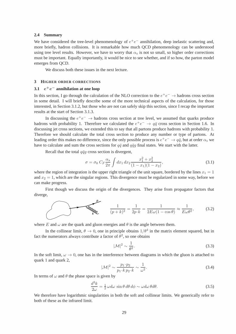
First though we discuss the origin of the divergences. They arise from propagator factors thatdiverge,
1
(p+ k)2=
1
2p·k =1
2Eω(1 − cos θ)≈ 1
Eωθ2, (3.2)
whereE andω are the quark and gluon energies andθ is the angle between them.
In the collinear limit,θ → 0, one in principle obtains1/θ4 in the matrix element squared, but infact the numerators always contribute a factor ofθ2, so one obtains
|M|2 ∼ 1
θ2. (3.3)
In the soft limit,ω → 0, one has in the interference between diagrams in which the gluon is attached toquark 1 and quark 2,
|M|2 ∼ p1 ·p2p1 ·k p2 ·k
∼ 1
ω2. (3.4)
In terms ofω andθ the phase space is given by
d3k
2ω= 1
2 ωdω sin θ dθ dφ ∼ ωdω θdθ. (3.5)
We therefore have logarithmic singularities in both the soft and collinear limits. We generically refer toboth of these as the infrared limit.
29
3.1.1 Regularization
As in the discussion of renormalization, the simplest way wecould regularize this cross section is witha cutoff, for example on the transverse momentum of the gluon, which would prevent the integrationentering both the soft and collinear regions. However, we will see that infrared singularities cancelbetween different contributions, in this caseqq andqqg, so we must use a regularization that can beconsistently applied in all contributions. It is not clear that this is the case for a cutoff, since it must beapplied in both real and virtual contributions, which have very different structures. Instead, to ensureconsistent application across all processes, it is better to modify the theory in such a way that somedimensionless parameterǫ regulates the divergences. Then the complete calculation can be performed inthis modified theory and at the end of the calculation, when all the divergences have cancelled, the limitǫ → 0 can be smoothly taken. Remarkably, dimensional regularization, which we used for ultravioletsingularities, also provides a consistent regulator for infrared singularities, as we shall discuss in detailshortly.
Another regularization scheme, which actually works well in QED, and for simple processes inQCD, is the gluon (or photon) mass regularization. We introduce a non-zero gluon massm2
g = ǫQ2.This prevents the propagators from reaching zero and diverging: for massless quarks the minimum valueism2
g and for a quark of massmq it is 2mqmg. With this modification one can recalculate the differentialcross section and integrate it to give a finite result,
σqqg = σ0 CFαs
2π
(
log21
ǫ− 3 log
1
ǫ+ 7− π2
3+O(ǫ)
)
. (3.6)
However, since a non-zero gluon mass violates gauge invariance, this method is bound to fail in general.In particular, it is not suitable for any process in which anylowest order contributions have externalgluons. As in the ultraviolet case, the only scheme that is known to be consistent with all the symmetriesof QCD, and hence to work to arbitrary orders in arbitrary processes, is dimensional regularization.
The reason why I said that it is remarkable that dimensional regularization works in the infraredlimit is the fact that the two limits have non-overlapping regions of applicability in the complexd plane.Ultraviolet-singular integrals are regularized by working in d < 4 dimensions, but infrared-singular inte-grals are only rendered finite by working ind > 4 dimensions. However, by carefully splitting contribu-tions that are singular in both the infrared and ultravioletone can consider the regularization schemes thatare used in each as independent. In each region, one considers the appropriate dimensionality (d = 4−2ǫwith ǫ > 0 in the ultraviolet and withǫ < 0 in the infrared) and then analytically continues to the wholecomplexǫ plane. Since analytical continuation is unique, this givesa unique result for each, in the regionof applicability of the other, and the two can be combined before the limitǫ → 0 is taken. This subtletyleads to some surprising results, for example for the self-energy of a massless quark, discussed below.
As the calculation of cross sections in dimensional regularization is rather technical, it is rare tosee it done in summer school lectures, but I think it brings out some interesting points, so I at leastsketch how the calculation works in Section 3.1.2. As I said,those who disagree can safely skip aheadto Section 3.1.3.
3.1.2 Aside: Real and virtual corrections in dimensional regularization
It is straightforward to generalize the Feynman rules tod dimensions and fairly straightforward to gener-alize the Dirac algebra. The result is thatd-dimensional matrix elements still have propagators∼ 1/p2,but that the numerators becomed dependent. (It is worth mentioning the closely-related dimensionalreduction scheme, which is often used for supersymmetry calculations, since conventional dimensionalregularization violates supersymmetry. In this scheme oneworks ind dimensions, but modifies the the-ory in such a way that fermions and massless vector bosons still have 2 spin states, instead ofd−2as in dimensional regularization. The result is that the matrix elements themselves are equal to the 4-
30
dimensional ones and it is only on performing the loop and phase space integrals that thed dimensionalitygets introduced.)
3.1.2.1 Phase space integralsWe will have to integrate overd-dimensional phase space. We beginby considering integer values ofd and then continue the results to real values. It is straightforward towrite down the basic integration measure,
ddk δ+(k2) =
dd−1k
2ω=
1
2ωd−3dω dΩd−2, (3.7)
whereω is the energy ofk anddΩd−2 is an element ofd−2-dimensional solid angle. The only difficultyconcerns the evaluation of integrals over this solid angle.In four dimensions we have
k = ω(1; sin φ sin θ, cosφ sin θ, cos θ) (4 dimensions), (3.8)
whereθ andφ are the usual spherical polar coordinates withθ the polar angle andφ the azimuthal angle.In five dimensions we have
k = ω(1; sinψ sinφ sin θ, cosψ sinφ sin θ, cosφ sin θ, cos θ) (5 dimensions), (3.9)
whereψ is an azimuthal angle in the additional dimension. Generalizing tod dimensions, we haved− 4additional azimuths and we writek generically as
k = ω(1; . . . , cosφ sin θ, cos θ) (d dimensions), (3.10)
where the ellipsis represents ad−3-vector of lengthsinφ sin θ containingd − 4 azimuths. Dependingon the complexity of the calculation, more or less of these additional components have to be specifiedprecisely. In fact in our case, since we only consider the relative orientations of three momenta that havezero total momentum, and therefore all lie in a plane, it is sufficient to specify
k = ω(1; . . . , cos θ) (d dimensions), (3.11)
where the ellipsis represents ad−2-vector of lengthsin θ containingd− 3 azimuths.
We can see how to integrate over the additional azimuths by again considering integerd and thengeneralizing,
∫
dΩ1 =
∫
dφ = 2π, (3.12)∫
dΩ2 =
∫
dφ sin θ dθ = 4π, (3.13)∫
dΩ3 =
∫
dψ sinφdφ sin2 θ dθ = 2π2, (3.14)
and so on. We have a recursion relation∫
dΩn =
∫
dΩn−1 sinn−1 θ dθ, (3.15)
which is solved by
Ωn ≡∫
dΩn =2π(n+1)/2
Γ[(n+ 1)/2]. (3.16)
We are now equipped to tackle the phase space integral, and see how the dimensional regularizationsucceeds in regularizing our integrals.
31
Fig. 3.1: One-loop diagrams fore+e− → qq
3.1.2.2 Regularization Since the form of the propagator factors is unchanged ind dimensions, and itis these that dominate the singular region, it is straightforward to read off the behaviour in the regularizedtheory. In the soft region we have
∫
0ω1−2ǫdω
1
ω2=
∫
0
dω
ω1+2ǫ∼ − 1
2ǫ, ǫ < 0, (3.17)
and in the collinear region∫
0sin1−2ǫ θ dθ
1
θ2∼∫
0
dθ
θ1−2ǫ∼ − 1
2ǫ, ǫ < 0. (3.18)
Since our cross section is divergent in both limits, and theycan overlap, i.e., a radiated gluon can be bothsoft and collinear, we expect the total cross section to be oforder1/ǫ2. Note, as a consistency check,that the integrands are positive definite and that, in the region in which they are well-defined,ǫ < 0, theresults are positive (and divergent asǫ→ 0).
3.1.2.3 Totale+e−
→ qqg cross section We now have all the ingredients we need to calculatethe differential cross section fore+e− → qqg and to integrate it over all phase space in dimensionalregularization. We obtain
σqqg = σ0 CFαs
2πH(ǫ)
(
2
ǫ2+
3
ǫ+
19
2− π2 +O(ǫ)
)
, (3.19)
whereσ0 is the lowest order cross section andH(ǫ) is a smooth function, withH(0) = 1, that we will notultimately need to know. Note that, as we anticipated from Eqs. (3.17) and (3.18), this result is positive,and divergent like1/ǫ2 asǫ→ 0.
So far, the regularization scheme has succeeded in quantifying the degree of divergence of the totalthree-parton cross section, but it has not helped us solve the problem of the divergence, by recovering afinite result for a physical cross section. As we already anticipated above, this will come by calculatingthe loop correction toe+e− → qq.
3.1.2.4 σ(e+e−
→ qq) at one loop We already made the point that to calculate the total cross sec-tion for e+e− → hadrons, we must sum over alle+e− → partons processes. At this order of perturbationtheoryqq is the only other process that contributes. There are three diagrams, shown in Fig. 3.1. Theyare down by one power ofαS relative to the tree-level diagram,
M1 ∝ αSM0. (3.20)
Therefore|M1|2 is two powers down and hence negligible at the order to which we are working. How-ever, since the final state is the same as that of the tree-level diagram, the two interfere, and their inter-ference,IReM∗
0M1 does contribute at orderαS.
32
In quantum mechanics, you know that we must sum over all unobserved quantum numbers at theamplitude level. Since the gluon momentum is unconstrainedby the outgoing quark momenta, we mustsum overall gluon momenta,
∫
ddk. (3.21)
Note that there is no mass-shell-constraining delta-function: the virtual integral is over all arbitrary on-and off-shell momenta.
We begin with the first two diagrams, which are proportional to the self-energy of a massless quark.It is actually easy to see that these have to be zero in dimensional regularization: the value of the integralhas dimensionsEd−4, but by Lorentz invariance the result of the integral can only be a function of thesquare of the quark’s momentum,p2 = 0, so there is nothing that can provide this dimensionality3.1.The only way these two facts can be reconciled is if the integral is zero. However, if we examine theintegrand somewhat closer, this is very surprising, because it is positive definite. How can a positivedefinite quantity integrate to zero?
The answer to this question comes from a subtle use of dimensional regularization. In fact thisintegral is divergent in both the infrared and ultraviolet.If we split the integral into two parts by introduc-ing an arbitrary separation scaleΛ, then we obtain an ultraviolet contribution∼ Λ−2ǫ/ǫ and an infraredcontribution∼ −Λ−2ǫ/ǫ. Each is positive in its domain of applicability (ǫ > 0 andǫ < 0 respectively),but after analytically continuing each to arbitraryǫ, they are exactly equal and opposite, giving a zeroresult for these diagrams.
Turning to the third diagram, the vertex correction, we find that it is also divergent in the infraredand ultraviolet regions. However, its ultraviolet divergence is exactly equal and opposite to the one fromthe sum of the two self-energy diagrams. Therefore the sum ofthe three diagrams is ultraviolet finite andno renormalization is needed at this order. This actually follows directly from the Ward identity of QED.Thus, one simply has to evaluate the vertex correction diagram in dimensional regularization, to obtainthe complete orderαS contribution toe+e− → qq. We find that the infrared divergences do not cancel,and we obtain
σqq = σ0 CFαs
2πH(ǫ)
(
− 2
ǫ2− 3
ǫ− 8 + π2 +O(ǫ)
)
. (3.22)
Dimensional regularization has succeeded in regularizingthe divergence of this contribution as well.This time, however, the result is negative and divergent asǫ → 0. This should not surprise us, as wealready noted that this is an interference term, so there is no requirement that it be positive, as there wasfor σqqg. In fact a quick glance at Eqs. (3.19) and 3.22) shows us that the divergences are going to cancelbetween them.
3.1.3 The total cross section
In the previous section we discussed how dimensional regularization provides finite results for the totalcross sections for thee+e− → qq ande+e− → qqg processes, which each diverge asǫ → 0. For thebenefit of those who slept through it, I restate them here:
σqq = σ0 CFαs
2πH(ǫ)
(
− 2
ǫ2− 3
ǫ− 8 + π2 +O(ǫ)
)
, (3.23)
σqqg = σ0 CFαs
2πH(ǫ)
(
2
ǫ2+
3
ǫ+
19
2− π2 +O(ǫ)
)
. (3.24)
According to our earlier discussion, the total cross section for e+e− → hadrons is given by the sum ofthe two. It is finite, so the limitǫ→ 0 can be taken,
3.1In fact this statement relies on working in a covariant gauge. In a lightcone gauge for example, the self-energy can dependonn·p. This diagram is not then zero, but of course the final answer for the sum of the three diagrams is gauge invariant.
33
σe+e−→hadrons = σ0
(
1 + CFαS
2π
3
2
)
(3.25)
= σ0
(
1 +αS
π
)
. (3.26)
Of course, this would be useless if it depended on the regularization procedure. The proof of its indepen-dence is beyond us here, but it is worth demonstrating it, by comparison with another scheme, the gluonmass regularization, in which we have
σqq = σ0CFαS
2π
[
− log21
ǫ+ 3 log
1
ǫ− 11
2+π2
3+O (ǫ)
]
, (3.27)
σqqg = σ0CFαS
2π
[
log21
ǫ− 3 log
1
ǫ+ 7− π2
3+O (ǫ)
]
, (3.28)
σhad = σ0
[
1 +αS
π
]
. (3.29)
Note that the individual cross sections have completely different forms in the different schemes, but thatthe sum of the two is scheme independent.
Equation (3.26) is one of the most fundamental quantities inQCD and is certainly one of themost well-calculated and measured. Despite the fact that itis a relative small correction to the total rate,experimental and theoretical systematic errors are so small that they can almost be neglected — evenwith the large statistics ofτ decays andZ decays at LEP, the statistical errors dominate. This means thatnot only does it provide one of the most accurate measurements, but its quoted accuracy is rather easyto interpret and implement in global analyses for example, unlike measurements that are dominated bysystematics.
Equation (3.26) is now known up to orderα3S. As discussed in Section 1.8, renormalization intro-
duces a renormalization scale dependence intoαs and the coefficient functions beyond the first one,
σe+e−→hadrons = σ0
(
1 +αS(µ)
π+C2
(
µ2
s
)(
αS(µ)
π
)2
+ C3
(
µ2
s
)(
αS(µ)
π
)3)
. (3.30)
Reducing this renormalization-scale dependence is one of the biggest reasons for going to higher orders.As can be seen in Fig. 3.2, the scale-dependence is indeed significantly smaller at each order, givingstability over a wider range ofµ. It can also be seen that providedµ is of orderQ, the higher ordercorrections are relatively small. We will see shortly that simply taking the leading order result withµ =
√s does surprisingly well and is certainly sufficient to understand the phenomenology.
3.1.4 αS measurements
As I mentioned above, the experimental measurement ofRe+e− gives one of the best measurementsof αs. In fact the LEP combined value ofRhad is
R(LEP ) = 20.767 ± 0.025, (3.31)
while the tree-level prediction isR0(Mz) = 19.984. (3.32)
Combining the two, and simply using the leading order resultwith µ =Mz, we obtain our first measure-ment ofαS,
αS(Mz) = 0.124 ± 0.004, (3.33)
surprisingly close to the value using the four-loop result [5], 0.119 ± 0.003.
As we discussed in Section 1.8.3, since QCD predicts the scale dependence ofαS, one measure-ment at any scale is sufficient to give a prediction for all scales. We can therefore phrase measurements
34
Fig. 3.2: The QCD prediction for the corrections toRe+e− at√s = 33 GeV as a function of renormalization scale
at leading, next-to-leading, and next-to-next-to-leading order, taken from ESW [1]
at other scales either as tests of QCD throughout the intervening energy range or, by translating them allinto measurements at a single scale, as different measurements of the same quantity that can be combinedto give a better overall measurement.
As an example, the average measurement ofR over several energy points around 34 GeV is
R(PETRA) = 3.88± 0.03, (3.34)
while the tree-level prediction isR0(34 GeV) = 3.69. (3.35)
Again using the leading order result, we obtain
αS(34 GeV) = 0.162 ± 0.026. (3.36)
Finally, using the one-loop renormalization group equation, we can convert this into a measurement ofαS(Mz),
αS(Mz) = 0.134 ± 0.018. (3.37)
This is in good agreement with the value from LEP, although with much larger uncertainties, simply dueto the fact that the statistics of the PETRA experiments weremuch lower.
As a final example, we considerτ decays. The QCD corrections to the hadronic decay rate actuallyhave two effects: on the ratio of branching fractions,Rτ , as discussed earlier, and also directly on thetotal decay rate of theτ . These can form the basis for two analyses in which the experimental errors arelargely independent. The combined result for the two is
αS(Mτ = 1.77 GeV) = 0.34 ± 0.01. (3.38)
This time, because we are translating over such a wide energyrange the one-loop renormalization groupequation does not do quite such a good job,
α(one-loop)S (Mz) = 0.1272 ± 0.0014, (3.39)
compared to the four-loop value [5]
αS(Mz) = 0.1212 ± 0.0011, (3.40)
35
0.1
0.15
0.2
0.25
0.3
0.35
0.4
0.45
α s(µ)
DIS
(B
j-SR
)D
IS (
GLS
-SR
)τ
deca
ys
QQ−
sta
tes
(latti
ce)
ϒ de
cays
e+e− (
σ had)
pp(−)
→bb−X, γX
e+e− (
jet &
eve
nt-s
hape
)
e+e− (
σ had)
e+e− (
jet &
eve
nt-s
hape
)
e+e− (
Z w
idth
)
e+e− (
jet &
eve
nt-s
hape
)
N3LON2LONLO
0.11
0.12
0.13
1 10 102
DIS (e/µ; F2)[1.9–15.2]
µ scale (GeV)
α s(M
Z)
Fig. 3.3: Results of a recent compilation ofαS values [5,6]
but it is not so far out. Note in this case the phenomenon of the‘incredible shrinking error’. Although themeasurement at theτ mass scale has a precision of about 3%, after evolving it toMz the relative uncer-tainty gets scaled down by the ratio of the twoαs values, andτ decays give the best single measurementof αs(Mz).
The results of a recent compilation [5, 6] are shown in Fig. 3.3. The scale dependence showsexcellent agreement with the predictions of perturbative QCD over a wide energy range. When translatedinto measurements ofαS(Mz), the separate measurements cluster strongly around the average value,
α(average)S (Mz) = 0.1204 ± 0.0009. (3.41)
3.2 Deep inelastic scattering revisited
The parton model I described in the last lecture assumed thatthe partons are non-interacting. But weknow that they do interact via QCD, so what will happen when weconsider these interactions? Wewill discover that the structure functions do become slowly(logarithmically) varying withQ2. We startby considering the next-to-leading order QCD corrections to quark scattering. We will find that these,if calculated naively, would be divergent, but that these divergences can be absorbed into the partondistribution functions. These will then become scale-dependent, giving rise to theQ2-dependence of thestructure functions.
3.2.1 NLO corrections to DIS
The next-to-leading order corrections come from three sources (recalling that we sum and integrate overall final statesX, so we must sum over all contributions in which any kind of parton is scattered):
1. One-loop corrections toeq → eq,
2. eq → eqg,
36
3. eg → eqq.
The third contribution is completely new in QCD and is not present in the parton model. We come backto it in a later section. The other two can more genuinely be thought of as higher-order corrections to theparton model process. We start with the second.
There are two contributing diagrams. The matrix element squared can be obtained by crossingfrom e+e− → qqg (1.66). Labeling the momenta as
e(k) + q(ηp) → e(k′) + q(p1) + g(p2), (3.42)
we obtain
∑
|M|2 =8CFNce
4e2qg2s
k ·k′ p1 ·p2 ηp·p2(
(p1 ·k)2 + (ηp·k)2 + (p1 ·k′)2 + (ηp·k′)2)
. (3.43)
As usual the phase space is given by (2.24),
dPS =Q2
16π2sx2dQ2 dx dPSX . (3.44)
This timeX consists of two partons so is non-trivial,
dPSX =d cos θ dφ
32π2, (3.45)
whereθ andφ refer to the direction ofp1 in the centre-of-mass system ofηp+q. It is conventional toreplacecos θ by the manifestly Lorentz-invariant variablez,
z ≡ p1 ·pq ·p = 1
2 (1− cos θ), (3.46)
with range0 < z < 1, giving
dPSX =dz dφ
16π2. (3.47)
It will later be instructive to know the transverse momentumof p1 in this frame,
k2⊥ = Q2(η
x− 1)
z(1− z). (3.48)
Note also that the caseη = x corresponds to a massless final state. Kinematically this can only happenif eitherp1 or p2 are infinitely soft (i.e., have zero energy), or if they are exactly collinear.
We therefore have
dσ2(e+ q)
dx dQ2=
1
4Nc
1
2s
Q2
16π2sx2
∫
dz dφ
16π28CFNce
4e2qg2s
k ·k′ p1 ·p2 ηp·p2(
(p1 ·k)2 + (ηp·k)2 + (p1 ·k′)2 + (ηp·k′)2)
.
(3.49)Rewriting in terms of our kinematic variables and averagingoverφ, we have
wherexp = x/η. Two things are already clear: at this order we will have a non-zero longitudinal struc-ture function,FL(x,Q
2); and thez integration, which runs from 0 to 1, will give a divergent contribution
37
to F2. This should worry us, since we are calculating a physical cross section, but let us continue for awhile and see what happens.
Putting everything together we have
dσ2(e+ q)
dx dQ2=CFα
2e2qαS
2ηx2y2s2
∫ 1
0dz
(
(1 + (1− y)2)
[
1 + x2p1− xp
1 + z2
1− z+ 3− z − xp + 11xpz
]
− y2
[
8zxp
])
,
(3.51)and hence
F2(x,Q2) =
∑
q
∫ 1
xdxp e
2q
x
xpfq
(
x
xp
)
CFαS
2π
∫ 1
0dz
(
1 + x2p1− xp
1 + z2
1− z+ 3− z − xp + 11xpz
)
.
(3.52)The divergence atz → 1 corresponds to kinematic configurations in which the outgoing gluon becomesexactly collinear with the incoming quark. Therefore in theFeynman diagram in which the gluon isattached to the incoming quark, the internal quark line becomes on-shell, causing the divergence. Notealso that the coefficient of the divergence itself diverges at the pointxp = 1, at which the gluon isinfinitely soft.
In order to study the divergence, let us first regulate it by calculating the contribution from emissionwith k2⊥ > µ2 (and assumeµ2 ≪ Q2 for simplicity). Sincek2⊥ is proportional to(1−z) this will give usfinite integrals. At any time, the full result can be obtainedby settingµ→ 0. We therefore obtain
F2(x,Q2) =
∑
q
∫ 1
xdxp e
2q
x
xpfq
(
x
xp
)
αS
2π
(
P (xp) logQ2
µ2+R(xp)
)
, (3.53)
where the functionR(xp) is finite. In the following we will not keep track of this function, although itwould be essential for quantitative analysis. The functionP (xp) we introduced in (3.53) is called thesplitting function (or more strictly speaking the unregularized splitting function),
P (x) = CF1 + x2
1− x. (3.54)
It actually describes the probability distribution of quarks produced in a splitting process,q → qg inwhich the produced quark has a fractionx of the original quark’s momentum. (We will quantify thisstatement slightly more shortly.)
Obviously by regulating the divergence we have not removed it: physical cross sections are stillsupposed to be obtained by settingµ → 0, in which caseF2 is logarithmically divergent. However,before discussing what happens to this divergence, let us consider the virtual one-loop correction toeq → eq. Since this diagram contains two quark-gluon couplings, when squared it would give anO(α2
S)correction. However, since it has the same final state as the lowest order diagram, we must consider theinterference between the two, and this interference isO(αS), so we must include it.
We could obtain the result for the one-loop diagram by crossing from e+e− → qq. However, toillustrate the physics, it is sufficient to recall a few of itsfeatures. Firstly, since the external particlesare the same as in the lowest-order process, the kinematics must be the same. In particular, it can onlycontribute at the pointη = x. Secondly, as in thee+e− case, the interference of the one-loop and tree-level diagrams is divergent and negative. In fact the kinematic regions in which the one-loop integranddiverges are exactly the same as those of theeq → eqg contribution we have just considered: when thegluon is soft, or is collinear with either of the quarks.
It turns out that the divergence is exactly right to cancel the one we obtained above atxp → 1. Infact one finds that after including the one-loop contribution, one gets exactly the same formula as (3.53)except that the unregularized splitting functionP (xp) is replaced by the regularized one,P (xp),
P (x) = P (x) + Pvirtual(x). (3.55)
38
Since the one-loop contribution has the same kinematics as the lowest-order process,Pvirtual(x) must beproportional toδ(1 − x). P (x) is therefore a distribution.
To define it, we will need to use a mathematical trick called the plus-distribution. Given somefunction f(x), which is well-defined for all0 ≤ x < 1, we define a distributionf(x)+ on the region0 ≤ x ≤ 1, as
f(x)+ = f(x)− δ(1 − x)
∫ 1
0dx′f(x′). (3.56)
The plus-distribution is most useful when the functionf(x) is divergent atx → 1. This means that forany other functiong(x), which is smooth atx = 1, we have the property
∫ 1
0dx f(x)+ g(x) =
∫ 1
0dx f(x) (g(x)− g(1)) . (3.57)
Provided thatg(x) goes tog(1) sufficiently quickly, this integral is finite.
After including the virtual contribution, the splitting function is given by
P (x) = CF
[
1 + x2
(1− x)++
3
2δ(1 − x)
]
. (3.58)
This is actually the first correction to a function that describes the momentum distribution of quarkswithin quarks,
P(x) ≡ δ(1 − x) +αS
2πlog
Q2
Q20
P (x) +O(α2S log
2), (3.59)
where the distribution is defined to be a pure quark at scaleQ0 and probed at scaleQ.
Inserting the full splitting function into (3.53), we find that the divergence atxp → 1 cancelsbetween the real and virtual terms, but the divergence forxp < 1 due to the regionz → 1 still remains.
3.2.2 Factorization of divergences
To understand why the results are still divergent even afterincluding the virtual terms, and what ulti-mately happens to the divergences, we consider their physical origin. Like thee+e− annihilation case,we have singularities from regions in which the real gluon iscollinear with either the incoming or out-going quark, or is soft, and also from the virtual graph, as illustrated in Fig. 3.4. All these contributionswere present ine+e− annihilation, but there we found that the divergences all cancelled to give a finitecontribution. Why is the present situation different? In fact we find that here the magnitudes of thedivergences are such as to cancel, but that the divergences arise in different regions of thexp integral, soare prevented from cancelling.
In thee+e− case, we argued that the singular regions of real emission were indistinguishable fromthe lowest order process, since an infinitely soft gluon could not produce any hadrons and the jets pro-duced by two collinear partons were indistinguishable froma single jet with their combined momentum.This statement is true here for the soft and final-state collinear contributions, but not the initial-statecontribution. The final state of this contribution is indeedindistinguishable from the lowest order pro-cess (it has an additional jet collinear with the outgoing proton remnant, but this too gives a jet andthe superposition of the two is indistinguishable from the proton remnant in the lowest order process).However, because we have used the parton model, we must convolute the partonic cross sections over anarbitrary (measured from experiment) probability distribution function, processes with different incom-ing momenta are effectively distinguishable. In all the singular regions, the final state of the process ismassless, and this fact fixes the incoming momentum (to the valueQ/2x in the Breit frame), but in theinitial-state singular process it is the internal line whose momentum gets fixed, as indicated in Fig. 3.4.Thus the incoming momentum in (c) is larger than in the other cases and its divergence, atη > x, cannotcancel the others, atη = x.
39
(a) (b)
(c) (d)
Fig. 3.4: Divergent contributions to DIS: (a) soft, (b) final-state collinear, (c) initial-state collinear, and (d) virtual.The labelp shows which momentum in each contribution is fixed by the massless final-state condition.
As I mentioned earlier, these divergences come from the virtuality of the internal particle van-ishing and hence the propagator diverging. Using the uncertainty principle, vanishingly small virtualitycorresponds to arbitrarily long time-scales. This seems tobe in direct contradiction with the assumptionunderlying the parton model, that the virtual photon takes an extremely rapid snapshot of the proton.
The problem is actually one of overcounting. We first introduced the pdfs, which are supposed tocontain all information about the internal structure of theproton. Presumably this internal structure isthe result of QCD interactions. We then tried to calculate the QCD corrections to the quark scatteringcross sections, integrating over all final states, so all energy-scales. But these QCD corrections shouldsomehow already be included in the internal dynamics of the proton.
To resolve this overcounting, we have to separate (or ‘factorize’) the different types of physics atdifferent energy scales. Like in our discussion of renormalization, I will first try to give the physicalpicture in terms of a cutoff, before returning later to describe how factorization works in practice indimensional regularization. We introduce the factorization scaleµ, and call all physics at scales belowµpart of the hadron wave function, and lump it into the parton distribution functions, and call all physicsat scales aboveµ part of the partonic scattering cross section (or ‘coefficient function’).
Therefore we do in fact have a transverse momentum cutoff in theeq → eqg process and the formof (3.53) is correct.
Since physics at scales belowµ is included in the pdfs and physics above is not, the pdfs them-selves must becomeµ-dependent. We therefore have
F2(x,Q2) =
∑
q
e2q
∫ 1
xdxp
x
xpfq
(
x
xp, µ2)
δ(1 − xp) +αS
2π
(
P (xp) logQ2
µ2+R(xp)
)
+O(α2S)
,
(3.60)where the functionR(xp) is not necessarily the same one as earlier, as the virtual contributions couldhave introduced some additional finite terms.
Note that the structure functions are nowQ2-dependent, violating Bjorken scaling. However,they also appear to beµ2 dependent, which should worry us:µ was introduced in a completely ad hoctheoretical way: it simply separates physical processes into two parts that are dealt with in different ways,and the final result, which is the sum of the two parts, should not depend on where the separation was
40
made. We return to discuss this point in more detail after calculating theµ2-dependence of the pdfs.
It is important to emphasize that, although we have derived these formulae for the higher ordercorrections to DIS, the leading logarithmic behaviour is universal. In particular, for any quark-inducedprocess with a hard scaleQ, we expect a hadronic cross section of the form
σh(ph) =∑
q
∫
dη fq(
η, µ2)
σq(ηph) +αS
2πlog
Q2
µ2
∫
dz P (z)σq(zηph)
, (3.61)
whereσq(p) is the partonic cross section for a quark of flavourq and momentump.
3.2.3 DGLAP evolution equation
Although the pdfs are fundamentally non-perturbative and cannot be predicted from first principles atpresent, physics at scales close toµ2 can be described perturbatively. We can therefore calculate theµ2-dependence of the pdfs so that, given their value at some starting scaleµ0, for example from experimentalmeasurements, we can calculate their values at all higher scalesµ.
To do this, we use the fact just noted, that physical cross sections should not depend onµ2. There-fore we should have
µ2dF2(x,Q
2)
dµ2= 0, (3.62)
or at least, since we are working atO(αS),
µ2dF2(x,Q
2)
dµ2= O(α2
S). (3.63)
Applying this to (3.60), we obtain
µ2d
dµ2fq(
x, µ2)
=αS
2π
∫ 1
x
dxpxp
fq
(
x
xp, µ2)
P (xp) +O(α2S). (3.64)
Equation (3.64) is called the Dokshitzer–Gribov–Lipatov–Altarelli–Parisi (or DGLAP, or GLAP, orAltarelli–Parisi for short) evolution equation. Note thatthe rate of change of the pdf at somex valuedepends on its value at all higherxs.
To understand its physical content, it is useful to rewrite the splitting function,
P (x) = CF
[
1 + x2
(1− x)++
3
2δ(1 − x)
]
= CF
(
1 + x2
1− x
)
+
, (3.65)
to give
µ2d
dµ2fq(
x, µ2)
= CFαS
2π
∫ 1
x
dxpxp
fq
(
x
xp, µ2)
1 + x2p1− xp
− CFαS
2πfq(
x, µ2)
∫ 1
0dxp
1 + x2p1− xp
. (3.66)
The first term represents the fact that the pdf at a givenx value is increased by quarks with higherx’s reducing their momentum fractions by radiating gluons. The second term represents the fact thatit is decreased by the quarks at thatx reducing their momentum fractions by radiating gluons. Eachcontribution is divergent due to emission withxp → 1, i.e., infinitely soft gluon emission, involving aninfinitely small change inx. However the two divergences exactly cancel because the number of quarksbeing lost to thisx value by infinitely soft gluon emission is equal to the numberbeing gained.
The DGLAP equation is most easily solved in moment space. Forany functionf(x), we define
fN =
∫ 1
0dxxN−1 f(x), (3.67)
41
the Mellin transform. Taking moments of both sides of (3.64), we obtain
µ2d
dµ2fqN
(
µ2)
=αS
2π
∫ 1
0dxxN−1
∫ 1
x
dxpxp
fq
(
x
xp, µ2)
P (xp) +O(α2S) (3.68)
=αS
2πPNfqN(µ2). (3.69)
It is common to introduce the notation
γN (αS) =αS
2πPN +O(α2
S), (3.70)
whereγN is known as the anomalous dimension. If we assume that the coupling αS is fixed, we caneasily solve (3.69) with the boundary condition of given values forfqN at some fixed scaleµ0,
fqN (µ2) = fqN (µ20)
(
µ2
µ20
)γN (αS)
. (3.71)
However, as we have seen, the renormalization of QCD means that the coupling constant becomesscale dependent,αS(µ
2), according to renormalization group equation
µ2d
dµ2αS(µ
2) = β(αS(µ2)) = −β0
2πα2
S(µ2) +O(α3
S). (3.72)
Inserting the solution of the running coupling, Eq. (1.73),into (3.69), we obtain
fqN (µ2) = fqN(µ20)
(
αS(µ0)
αS(µ)
)
PNβ0
. (3.73)
Having the solution forfq in momentN -space, we have to convert it back tox-space. This is doneby the Inverse Mellin Transform, wherefqN is continued to the complex plane,
fq(x) =1
2πi
∫
CdN fqN x
−N , (3.74)
where the contourC runs parallel to the imaginary axis to the right of all poles.Because of the complexityof this process, the DGLAP equation is often solved simply by‘brute force’ numerical solution of (3.64).
BeyondO(αS) the general structure of (3.69) and (3.72) remains unchanged: the anomalous di-mension andβ function simply become power series inαS.
3.2.4 Scheme/scale dependence
Factorization, as introduced above, may seem pretty arbitrary. However it can be proved to all orders inperturbation theory. The most convenient way to do this is touse, instead of the transverse momentumcutoff we used above, dimensional regularization. When we calculate the NLO cross section ind dimen-sions, the divergence shows up as a pole,1/ǫ. The coefficient multiplying this pole turns out to be thesame splitting function we encountered earlier.
In d dimensions, we obtain for the structure function up toO(αS),
F2(x,Q2) =
∑
q
e2q
∫ 1
xdxp
x
xpfq
(
x
xp
)
δ(1 − xp) +αS
2π
((
4πµ2
Q2
)ǫ −1
ǫP (xp) +R(xp)
)
+O(ǫ)
,
(3.75)whereµ is the scale introduced to make the coupling constant dimensionless. Note that I have sneakilyadded a bar tofq and that it is scale independent.fq is known as the bare pdf. We now note that the
42
distribution functions themselves are not physical observables, only their convolution with coefficientfunctions is. I can therefore define a modified set of distribution functions as follows:
x fq(x) ≡∫ 1
xdxp
x
xpfq
(
x
xp, µ2F
)
δ(1− xp)−αS
2π
((
4πµ2
µ2F
)ǫ −1
ǫP (xp) +K(xp)
)
, (3.76)
whereµF is the (completely arbitrary again) factorization scale, and K(xp) is a completely arbitraryfinite function to be discussed shortly. (To fit in with the standard notation, I should really multiply alloccurrences ofαS by 1/Γ(1 − ǫ) = 1 − γEǫ + O(ǫ2), but this will merely change the values ofR(xp)andK(xp) which I do not specify anyway.) Combining (3.75) and (3.76),we end up with
F2(x,Q2) =
∑
q
e2q
∫ 1
xdxp
x
xpfq
(
x
xp, µ2F
)
δ(1 − xp)
+αS
2π
(
P (xp) logQ2
µ2F+R(xp)−K(xp)
)
+O(α2S)
. (3.77)
Note that this has the identical form to (3.60), except for the finite function. It is clear from (3.76) thatfq(x, µ
2F ) depends on the functionK(xp). It therefore seems like we have no predictive power: the
pdf and coefficient function each depend on the completely arbitrary functionK(xp) and the completelyarbitrary scaleµF (note that all dependence onµ has again completely cancelled. As I said in the contextof renormalization, many textbooks simply set it equalµ right from the start, but I consider this slightlyconfusing as they have quite different physical meaning. Having performed this manoeuvre, I henceforthdrop the subscriptF ). However, the factorization theorem proves, firstly that for any physical quantity,all dependence onK(xp) andµ will cancel and secondly that the scheme- and scale-dependent pdfs,fq(x, µ
2) are universal (i.e., process-independent).
Two schemes are in common use, theMS scheme in whichK(xp) is zero, and the DIS scheme inwhichK(xp) = R(xp), i.e. in which forµ = Q the parton model result is exact.
To understand the physical content of the scheme-dependence, it is worth while going back to thecase with a cutoff. If, instead of a cut on transverse momentum we had used a cut on the virtuality of theinternal quark line to separate the pdf from the coefficient function, we would have got exactly the sameform as (3.60) except thatR(xp) would have been a different function. In particular, it would differ by alog[(1− xp)/xp] term, together with some non-logarithmic terms. In fact, all logarithmic terms turn outto be the same with apt cutoff as in theMS scheme, so for many purposes the two can be consideredequivalent.
Although dependence on the scheme and scale must cancel in physical quantities, it is only guar-anteed to do so after calculating to infinite orders of perturbation theory. At any finite order there can besome residual dependence. We must therefore have a procedure for choosing a value ofµ. Essentiallythe identical discussion we had for the renormalization scale choice applies here. One can show that astructure like (3.60) continues to all orders of perturbation theory and that for every power ofαS, onegets a power oflogQ2/µ2. Thus every order of perturbation theory contains terms likeαn
S logmQ2/µ2,
m ≤ n. It is clear that ifµ is a long way fromQ, the log can be large enough to compensate the smallnessof αS and the perturbative series will not converge quickly. One should therefore chooseµ ‘not too far’fromQ.
It is worth mentioning that one can set up DGLAP evolution equations for theQ2-dependenceof the structure functions,F2 andFL, themselves. These are then automatically scheme- and scale-independent even at finite orders of perturbation theory. This is sometimes known as the scheme-independent scheme.
43
Pqq(x) = CF
[
1 + x2
(1− x)++
3
2δ(1 − x)
]
Pqg(x) = TR
[
x2 + (1− x)2
]
Pgq(x) = CF
[
1 + (1− x)2
x
]
Pgg(x) = CA
[
2x
(1− x)++ 2
1− x
x+ 2x(1 − x)
]
+β0δ(1 − x)
Fig. 3.5: The four DGLAP splitting functions of QCD
3.2.5 Initial-state gluons
As mentioned right at the start of this section, we also obtain O(αS) corrections from the processeg →eqq. Most of what we said above carries over in a straightforwardway. Although there is no softsingularity or virtual term to cancel it, there is a collinear singularity. This corresponds to a two-stepprocess in which a gluon splits to aq–q pair, one of which interacts with the photon. The singularityagain corresponds to the virtuality of the internal quark line going to zero. This singularity can again beabsorbed into a factorized universal pdf for the gluon. We end up with an additional contribution to thestructure function of
F2(x,Q2) =
∑
q
e2q
∫ 1
xdxp
x
xpfg
(
x
xp, µ2)
αS
2π
(
Pqg(xp) logQ2
µ2+Rg(xp)−Kqg(xp)
)
+O(α2S)
,
(3.78)where the sum overq is over all ‘light’ flavours. We now have four different typesof splitting function,illustrated in Fig. 3.5. The DGLAP equation now becomes a setof coupled equations:
µ2d
dµ2fa(
x, µ2)
=∑
b
αS
2π
∫ 1
x
dxpxp
fb
(
x
xp, µ2)
Pab(xp) +O(α2S). (3.79)
In moment space, this can be conveniently written as a matrixequation (in general of(2Nf+1)×(2Nf+1)matrices, but for simplicity we show the case of only one flavour of quark):
Exactly the same solution is obtained, but in matrix notation,
fqN (µ2)fqN (µ2)fgN (µ2)
= exp
∫ µ2
µ20
dµ′2
µ′2
γqqN (αS(µ′)) 0 γqgN (αS(µ
′))0 γqqN (αS(µ
′)) γqgN (αS(µ′))
γgqN (αS(µ′)) γgqN (αS(µ
′)) γggN (αS(µ′))
fqN (µ20)fqN (µ20)fgN (µ20)
.
(3.81)This is even more troublesome to do by the Inverse Mellin Transform, so the full set of DGLAP equationsis almost always solved numerically.
Note that at higher orders of perturbation theory, even the zero entries in (3.80) become non-zero,as do contributions likePqq′(x).
44
1
10
F2
x=1.3E-05 (x 18)
x=2E-05 (x 10)
x=3.2E-05 (x 4)
x=5E-05 (x 2)
x=8E-05 (x 1)
H1SVX95H194H195NVX prel.H196NVX prel.E665NMCBCDMS
H1 QCDFit96 prel
1
10
x=0.00013 (x 10)
x=0.0002 (x 5)
x=0.00032 (x 3)
x=0.0005 (x 1.8)
x=0.0008 (x 0.8)
x=0.0013 (x 12)
x=0.002 (x 8)
x=0.0032 (x 4)
x=0.005 (x 2.2)
x=0.008 (x 1.3)
1
10
10-1
1 10 102
103
104
x=0.013 (x 18)
x=0.02 (x 10)
x=0.032 (x 6)
x=0.05 (x 3.5)
x=0.08 (x 2)
10-1
1 10 102
103
104
Q2 [GeV2]
x=0.13(x 32)
x=0.2(x 16)
x=0.32(x 8)
x=0.5(x 6)
Fig. 3.6: Fit to theF2 data over a wide range ofQ2 values, exhibiting violation of Bjorken scaling
3.2.6 Violation of Bjorken scaling
As we already noted, the factorization of initial-state singularities introduces a logarithmicQ2 depen-dence into the structure functions and therefore a slow violation of Bjorken scaling. There is a closeanalogy with the renormalization of one-scale cross sections, where the energy-dependence was entirelydue to the quantum corrections. Although the pdfs at some lowscale are entirely non-perturbative andmust be fit to data, the scale-dependence is entirely predicted by QCD and provides a stringent test overa wide range of energy scales. The result is impressive, see Fig. 3.6.
3.3 Summary
NLO calculations are hard! This is mainly because the real and virtual corrections are each divergentand must be regularized in some self-consistent way, for example with dimensional regularization. Un-like the ultraviolet divergences, which are isolated in well-localized pieces of the loop calculation andcan effectively be removed by a redefinition of the Feynman rules, these divergences arise in differentpartonic contributions to physical observables. They musttherefore be kept explicit until the very end ofthe calculation when all the partonic contributions are combined. Only then, provided our observable isinfrared safe, will the real and virtual divergences cancelto yield a finite result.
Processes with incoming partons have extra divergences, arising from a miscancellation of theinitial-state-collinear real and virtual contributions,which appear at different points in the integral overincoming momentum fraction. (It is worth mentioning that the same argument applies to the final-statedistributions of identified hadrons, for example the momentum distribution of pions produced ine+e−
annihilation.) These divergences have to be factorized into the non-perturbative, but universal, partondistribution functions at some factorization scaleµF . This extra scale in the structure functions allowsthem to beQ2-dependent. ThisQ2-dependence is entirely driven by theµ2F -dependence of the partondistribution functions, which is predicted by the DGLAP evolution equations. Thus structure functiondata over a wide range ofQ2 provide a stringent test of perturbative QCD.
45
4 SUMMARY
In this short course on QCD phenomenology, I have resisted the temptation to review the many importanttests and studies of QCD that have been made over the years andhave instead tried to concentrate on thekey ideas that underpin them. These are:
– The gauge invariance of the theory, which allows us to writedown the Lagrangian and whichpredicts some of the most important features of the theory: the universality of the coupling constantand the self-coupling of gluons, which ultimately leads to the negativeβ function and hence toasymptotic freedom at high energies and strong interactions at low energies.
– Renormalization and decoupling, which allow us to make predictive calculations at finite en-ergy, without knowing the full structure of the theory to arbitrarily high energy and without theintroduction of arbitrarily many input parameters. Renormalization is related to the quantumstructure of the theory and introduces a dimensionful scaleinto even the scaleless Lagrangian ofmassless QCD, giving rise to energy-dependence of one-scale observables that would be energy-independent in the classical theory.
– Factorization and evolution, which allow us to use perturbation theory to calculate the interactionsof hadrons, since all the non-perturbative physics gets factorized, into universal functions that canbe measured in one process, like DIS, and then used to predictthe cross sections for any otherprocess. Again, this introduces a scale dependence into theparton model so that the structurefunctions of DIS, and other one-scale observables such as the Drell–Yan cross section, becomescale dependent.
– Infrared safety, which ensure that the infrared singularities associated with soft and collinear emis-sion cancel between real and virtual contributions, allowing the perturbative calculation of jet crosssections, without a detailed understanding of the mechanism by which partons become jets.
Together, these allow us to make sense of QCD, without havingto solve the theory at all possible scales:unknown or uncalculable high- and low-energy effects can berenormalized, factorized and cancelledaway. After all this, it is remarkable that most QCD phenomenology can be understood at least qual-itatively from leading order perturbation theory with the one-loop renormalization group and DGLAPevolution equations. Higher order corrections, while essential for quantitative analysis, do not changethis simple picture dramatically.
ACKNOWLEDGEMENTS
It is a pleasure to acknowledge the organizers, lecturers, tutors and students of the Latin AmericanSchool of High Energy Physics at Recinto Quirama for making giving these lectures such an enjoyableexperience.
REFERENCES
[1] R.K. Ellis, W.J. Stirling, and B.R. Webber,QCD and Collider Physics, Cambridge Monographs onParticle Physics, Nuclear Physics and Cosmology, Volume 8 (Cambridge University Press, 1996).
[2] M.E. Peskin and D.V. Schroeder,An Introduction to Quantum Field Theory(Addison-Wesley,1995).
[3] M. Gockeler, R. Horsley, A. C. Irving, D. Pleiter, P. E. L.Rakow, G. Schierholz, and H. Stuben,A determination of the Lambda parameter from full lattice QCD, Phys. Rev. D73 (2006) 014513[arXiv:hep-ph/0502212].
[4] M. Davier, S. Eidelman, A. Hocker, and Z. Zhang,Confronting spectral functions from e+ e- anni-hilation and tau decays: Consequences for the muon magneticmoment, Eur. Phys. J. C27 (2003)497 [arXiv:hep-ph/0208177].
[5] M. Davier, S. Descotes-Genon, A. Hocker, B. Malaescu, and Z. Zhang,The determination ofαs
from τ decays revisited, Eur. Phys. J. C56 (2008) 305 [arXiv:0803.0979 [hep-ph]].
[6] S. Bethke, Experimental tests of asymptotic freedom, Prog. Part. Nucl. Phys.58 (2007) 351[arXiv:hep-ex/0606035].