arXiv:hep-th/0205252v3 2 Sep 2002 The Higgs Field As The Cheshire Cat And His Yang-Mills ”Smiles” L. D. Lantsman Wissenschaftliche Gesellschaft, bei Judische Gemeinde zu Rostock, Wilhelm-K¨ ulz Platz,6, 18055, Rostock,Germany; [email protected]V. N. Pervushin Bogoliubov Laboratory of Theoretical Physics, Joint Institute for Nuclear Research, 141980 Dubna, Russia; [email protected]May 19, 2018 Abstract The well-known Bogomol’nyi-Prasad-Sommerfeld (BPS) monopole is considered in the limit of the infinite mass of the Higgs field as a basis of the Yang-Mills field vacuum with the finite energy density. In this limit the Higgs field disappears, but it leaves its trace as the BPS monopole transformed into the Wu-Yang monopole obtained in the pure Yang-Mills theory by a spontaneous scale symmetry breaking in the class of functions with the zero value of the topological charge. The topo- logical degeneration of the BPS monopole manifests itself as Gribov copies of the covariant Coulomb gauge in the form of the time integral of the Gauss constraint. We also show that, in the considered theory, there is a zero mode of the Gauss constraint leading to an electric monopole and an additional mass of η ′ -meson in QCD. The consequences of the monopole vacuum in the form of a rising potential and topological confinement are studied in the framework of the perturbation the- ory. An estimation of the vacuum expectation value of the square of the magnetic tension is given through the η ′ -meson mass, and arguments in favour of the stability of the monopole vacuum are considered. We also discuss why all these ”smiles” of the Cheshire cat are kept by the Dirac fundamental quantization, but not by the conventional Faddeev-Popov integral. 1
Transcript
arX
iv:h
ep-t
h/02
0525
2v3
2 S
ep 2
002
The Higgs Field As The Cheshire Cat
And His Yang-Mills ”Smiles”
L. D. LantsmanWissenschaftliche Gesellschaft, bei Judische Gemeinde zu Rostock,
The well-known Bogomol’nyi-Prasad-Sommerfeld (BPS) monopole is consideredin the limit of the infinite mass of the Higgs field as a basis of the Yang-Mills fieldvacuum with the finite energy density. In this limit the Higgs field disappears, butit leaves its trace as the BPS monopole transformed into the Wu-Yang monopoleobtained in the pure Yang-Mills theory by a spontaneous scale symmetry breakingin the class of functions with the zero value of the topological charge. The topo-logical degeneration of the BPS monopole manifests itself as Gribov copies of thecovariant Coulomb gauge in the form of the time integral of the Gauss constraint.We also show that, in the considered theory, there is a zero mode of the Gaussconstraint leading to an electric monopole and an additional mass of η′-meson inQCD. The consequences of the monopole vacuum in the form of a rising potentialand topological confinement are studied in the framework of the perturbation the-ory. An estimation of the vacuum expectation value of the square of the magnetictension is given through the η′-meson mass, and arguments in favour of the stabilityof the monopole vacuum are considered. We also discuss why all these ”smiles” ofthe Cheshire cat are kept by the Dirac fundamental quantization, but not by theconventional Faddeev-Popov integral.
The nature of the vacuum of the Yang-Mills (YM) theory in the Minkowski space is anopen problem at the present time. There were a lot of attempts to solve this problem.
A typical feature of these attempts was the construction of the nontrivial physicalvacuum in the Minkowski space on the basis of nonzero values of vacuum expectationscoinciding with statistical averages (classical fields). As an example of these attempts weshould like to point out the work [1] stimulated by the asymptotic freedom formula as acriterion for instability of the naive perturbation theory [2]. However, these attempts didnot take account of the topological structure of vacuum.
This structure of the vacuum of the Yang-Mills theory was discovered in the Euclideanspace [3], and it means that there exist classical in-, out-vacuum states correspondingto different topological indices |n > with zero values of energy, and tunnel transitions|n >→ |n + 1 > occur between them. These transitions are described by instantons, i.e.Yang-Mills fields with fixed topological numbers ν = nout − nin satisfying the minimumof the Yang-Mills action. A defect of this vacuum is non-physical status of a zero valueof energy in quantum theory. However, the topological degeneration of initial data forYang-Mills fields does not depend on the space where these fields are considered. Theinitial data of any classical solution in the Minkowski space-time are also topologicallydegenerated. It is worth to investigate topologically degenerated vacuum solutions inthe Minkowski space-time in the class of functions with physical values of finite energydensities.
The present paper is devoted to just this investigation of the nontrivial topologicalvacuum of the Yang-Mills theory in the Minkowski space-time. This vacuum is stipulatedby the fact that the homotopy groups of all the 3-dimensional paths (loops) on the SU(2)group manifold are nontrivial (p.325 in [4]):
π3(SU(2)) = Z. (1.1)
The Yang-Mills vacuum should take account of this topology. We investigate the topologi-cal degeneration of the initial data using the well-known Bogomol’nyi-Prasad-Sommerfeld(BPS) monopole as an example. This monopole is a result of the spontaneous break-downof the SU(2) symmetry on the basis of the classical Higgs field φ0 (i.e. the λφ
4 theory) inthe limit λ→ 0. This means that we consider the ideal Bose gas of scalar Higgs particles.This Bose gas is called the Bose condensate. The Higgs Bose condensate has a directanalogy with Bose condensate in the theory of superfluid helium [5].
Thus, there is the possibility to construct the YM vacuum using the well-known Bosecondensate of free scalar particles in the limit of their infinite mass when these particlesdisappear from the spectrum of elementary excitations of the theory leaving their ”traces”in the form of monopoles. The study of these ”traces” is the aim of the present paper.
One of these ”traces” is the topological degeneration of the BPS monopole perturba-tion theory that manifests itself as Gribov copies of the covariant Coulomb gauge treatedas initial data of the Gauss constraint in the lowest order of the perturbation theory withthe new monopole vacuum. The Gribov copies mean that there is a zero mode of the
2
Gauss law constraint expressed through the global variable N(t) that describes a topolog-ical motion of the Yang-Mills Bose condensate as a whole system with the real momentumspectrum.
We construct the generating functional for weak perturbation excitations over thisvacuum in the form of the Feynman path integral.
The paper is organized as follows:Section 2 is devoted to a brief review of the problem of vacuum in quantum-field
theories. We discuss what the vacuum is in such theories and the ways of symmetrybreak-down, which were very fruitful in modern physics.
Further we give the general picture of the symmetry break-down and its connectionwith the nonzero vacuum expectation value < 0|φ|0 > 6= 0 with the example of the λφ4
theory.In the conclusion of Section 2 we show that the Higgs sector of the Yang-Mills theory
in the BPS limit λ→ 0 leads to nontrivial monopole solutions of the equations of motionwith a finite energy density corresponding to the SU(2) → U(1) spontaneous break-down.The Bogomol’nyi equation, defining the lowest level of the monopole energy, determinesthe direct connection between Yang-Mills and Higgs multiplets. This will be a startingpoint for the construction of a consistent theory of the Yang-Mills vacuum in Section 4.
Section 3 is devoted to the construction of the Dirac variables in the Yang-Mills theoryin the form of solutions of the Gauss constraint-shell equation. This will be the base ofall our further consideration.
The topological degeneration of the initial data is the subject of Section 4. We arguein favour of that the vacuum in the ”old” instanton approach is not the physical one.Instead, we construct the monopole Φ
(0)i (x) in the form of the stationary Bose condensate
with the topological number 0 and the nonzero ”magnetic” tension B(Φ(0)i ) corresponding
this monopole. All this is a result of the SU(2) spontaneous break-down, describing bythe classical equations of the non-Abelian theory in the class of fields with the topologicalnumber 0. These equations have nontrivial solutions in the form of Wu-Yang monopoles:Φ
(0)i (x). Our construction of the YM vacuum is only a presentation of such solutions as
BPS monopoles in the theory with Higss fields in the limit of their infinite masses, but withthe finite energy density; so that the BPS ”magnetic” tension B(Φ
(0)i ) (in this limit) has
itself a crucial importance. We show that in the considered limit the Gibbs expectationvalue < B2 > (defined as the averaging B2 over the volume) can be different from zero;it is a direct analogy with the Meisner effect in a superconductor. In the language of thegroup theory, it means the spontaneous break-down of the U(1) group. This, in turn, isa precondition for the correct consideration of the η′-meson problem in QCD. A nonzerovalue of < B2 > allows also us to regularize our theory by the introducing of an infraredcut-off parameter ǫ(< B2 >) that plays the role of the size of the BPS monopole.
The goal of Section 4 is to show the nature of the topological degeneration of themonopole Φ
(0)i (x) as the Gribov ambiguity of the covariant Coulomb gauge (in the form
of the time integral of the Gauss constraint). This topological degeneration is defined
by the non-perturbation factor exp(nΦ(0)0 (x)), where Φ
(0)0 (x) is a solution of the Gribov
ambiguity equation that coincides with the Higgs field in the form of a BPS monopole.
3
As the covariant Coulomb gauge is the time integral of the Gauss law constraint, theGribov ambiguity signals that there are zero modes of the Gauss constraint considered asthe equation for the time component Ac
0(t,x) of the Yang-Mills field.The in the main new step in our investigation is the introduction of the non-integer,
continuous topological variable N(t) for the definition of the zero mode of the solution of
the Gauss law constraint for Ac0(t,x) in the form of the product N(t)Φ
(0)c0 (x). This zero
mode induces the ”electric” tension (”electric monopole”) as a dynamic degree of freedomthat cannot be removed by fixing of any gauge. This ”electric” tension, in turn, generatesthe action of a free rotator describing the global rotation of the Yang-Mills vacuum as awhole system. The corresponding Schrodinger equation for vacuum has the real spectrumof momenta in contrast with the instanton case. The dependence of the rotator action onthe Gibbs expectation value < B2 >, which, in turn, depends on the Higgs mass (throughthe Bogomol’nyi equation), confirms our suggestion about the Yang-Mills vacuum as aBose condensate.
The topic of Section 5 is a more detailed analysis of zero modes of the covariantCoulomb gauge and the Yang-Mills (constraint-shell) action; also we decompose the ”elec-tric” tension into the transverse and the longitudinal parts with respect to the constraint-shell equation.
Section 6 is devoted to the calculation of the instantaneous potential of the current-current interaction in the presence of the Wu-Yang monopole. Instead of the Coulombpotential in QED, the corresponding Yang-Mills Green function take the form of the sumof the two potentials: the Coulomb potential and the rising one; it is of great importancefor the analysis of the hadronization, in particular of the η′-meson problem.
The analysis of the Feynman and FP path integrals is the subject of Section 7.The last two Sections, 8 and 9, are devoted to the analysis of the topological confine-
ment and the quark confinement in QCD as direct consequences of the average over thetopological degeneration.
The theory considered in Sections 8 allow us to contend that only the colourless(”hadronic”) states form a complete set of physical states in QCD. We prove that thetopological confinement leads to the quarks confinement in QCD, that the complete setof hadronic states ensures that QCD is an unitary theory. In Section 10 we estimate thevalue of the vacuum chromomagnetic field in QCD(3+1).
2 Vacuum as a result of spontaneous symmetry break-
down.
2.1 A physical vacuum as a Bose condensate.
All quantum -field theories are considered in the Hilbert-Fock space of second quantization(see §7.3 in [6] and [7]). It is quite logical to begin our consideration with a suitableabstract mathematical model (p.40 in [6]). So, let some algebra with involution U begiven (the creation - annihilation operators are examples of an algebra of that sort). We
4
denote this algebra by C∗. One constructs the C∗ - homomorphism π of the C∗ - algebraU into the algebra B(H) of all the linear restricted operators defined in the Hilbert spaceH. The homomorphism π is called the representation of the C∗-algebra U in the Hilbertspace H. The representation π is called the irreducible one, if every closed subspace inH, invariant with respect to all the operators π(A)(A ∈ U), is ∅ or the whole Hilbertspace H. The vector Φ ∈ H is called the cyclic vector for the representation π, if all thevectors of the form π(A)Φ, where A ∈ U , form a complete set (a linear shell ) in H. Thisrepresentation with the cyclic vector is called the cyclic one.
If Φ is a vector in H, then it generates the positive functional
FΦ =< Φ, π(A)Φ > (2.1)
on U (in terms of the probability theory it is the mathematical expectation of the valueπ(A) in the state Φ). This functional is called the vector functional associated with therepresentation π and the vector Φ.
In these terms the Gelfand-Naimark- Sigal (GNS) construction of a vacuum (p.42 in[6]) consists in the following: one can determine some (cyclic) representation πF of thealgebra U in the given Hilbert space with the cyclic vector ΦF for the given positivefunctional F such that
F (A) =< ΦF , πF (A)ΦF > . (2.2)
The representation πF is determined with these conditions as unique to within the unitaryequivalence. This construction of the cyclic vector ΦF as the vacuum vector (or simplythe vacuum) allowed us to write down the theory of second quantization.
Let us consider the free (i.e. without an interaction) theory of one particle (boson).This boson has its fixed integer spin s and mass m (therefore also the fixed square ofthe Pauli-Lubanski vector W 2 = m2s(s + 1), and its mass-shell equation is p2 = m2).As usual in quantum -field theories, we place our particle in a large enough closed box.Then, according to the Hilbert-Schmidt theorem (p.231 in [8]), the momentum spectrumof the particle is discrete.
Associating the ortho-normalized vectors of some infinite-dimensional Hilbert spacewith the quantum numbers of the momentum and spin (helicity), we obtain the one-particle Hilbert (Fock )space (at the level of special relativity), which we denote as Σ[m,s].
Let some algebra with involution (depending on the momentum p and spin s) be givenin the form of the Bose commutation relations of the operators a(p), a†(p) (the formula(4.16) in [9]):
[a(p), a†(p)] = (2π)32ωpδ3(p− p′) , (2.3)
where ωp is the frequency corresponding to the momentum p, and
[a(p), a(p′)] = [a†(p), a†(p′)] = 0. (2.4)
We suppose that the operator a†(p) acts on the vacuum vector (which we shall denotesometimes as |0 >) as
a†(p)|0 >= Φ(p) (2.5)
5
for the eigenvalue p of the momentum operator. All such vectors, depending on p (andthe value of helicity), form a linear shell of our H = Σ[m,s]. It is said that the boson withthe momentum p and spin s (at a fixed helicity) was created from the vacuum |0 >.
Operator a(p) has a contrary action on the vacuum |0 >. This action is expressed as
a(p)|0 >= 0 , (2.6)
and we say that the operator a(p) annihilates the vacuum |0 >.The considered simple example shows us how one can introduce the vacuum into some
quantum-field theory. This is a purely mathematical construction, and this vacuum iscalled the mathematical one. But, to construct a consistent relativistic quantum-fieldtheory, we should impose some conditions on its vacuum.
First of all, this is the condition that the vacuum exists and is unique to within aphase factor. The mentioned phase factor should preserve the (unit) norm of the vacuumvector. Thus, this factor has the form exp(iφ), and we already have some degeneration ofthe vacuum with respect to the Abelian U(1) group.
Then we demand that our vacuum should be invariant with respect to pure Poincaretranslations U(a, 1) (p.251 in[6]). This leads, as a final result, to the conservation of themomentum-energy tensor of the theory. We associate always the minimum value of energywith the vacuum vector Φ0 ∈ H. We call the state with the minimum value of energy theground physical state. Note that,in the free quantum -field theory, the spectrum of themomentum-energy operator P belongs to the set V +
µ
⋃{0}, where V +m = {p ∈ M : p2 ≥
m2, p0 > 0} at m ≥ 0 and M is the Minkowski space (the so-called strict condition ofspectrality).
All the states are considered as (perturbation) excitations over the vacuum. We shallutilize this fact in our present work.
The condition that vacuum is invariant with respect to pure Poincare translations issatisfied when P = 0. All the states with such P are invariant under pure Poincare trans-lations. All the unitary representations of this class, except for the unit representation,the vacuum (U(a, Λ) ≡ 1, where Λ ∈ SL(2, C)) are infinite-dimensional with respect tothe 3-dimensional SO(3) rotations.
We say that the cluster feature (or the feature of the asymptotic factorisation) is fulfilledin the physical Hilbert space H if there exists the vector of unit norm Ψ0 ∈ H such that
< Φ, U(λa, 1)Ψ > → < Φ,Ψ0 >< Ψ0,Ψ >, λ→ ∞ , (2.7)
where a is an arbitrary space-like vector in the Minkowski space M ; Φ,Ψ ∈ H.It turns out that the condition that the vacuum exists and is unique is equivalent to
the cluster feature (2.7).Let us consider (p.294 in [6]) some quantum field φ and let us supply it with the index
κ (φ(κ)) which defines the type of this field (for example its spin). Thus, every φ(κ) is a
tensor or a spin-tensor with a finite number of its Lorentz components: φ(κ)l (l = 1, ..., rκ)
and with a definite transformation features with respect to the eigen Lorentz group L↑+
or its covering SL(2, C).
6
In these terms we can construct a consistent relativistic quantum field theory if itsvacuum is cyclic in the following sense. The set D0 of finite linear combinations of (spin)-
tensor fields of the form φ(κ1)l1
(f1)... φ(κn)ln
(fn)|0 > is dense in H.A very important role in quantum-field theories plays the vacuum expectation value
of some quantum field φ over the vacuum < 0|φ|0 >. But this value is zero at the levelof the algebra of creation-annihilation operators a(p), a†(p′) in the Fock-Hilbert space ofsecond quantization: because of the relation (2.6).
Now, with the help of simple arguments, we shall show the connection of the relation< 0|φ|0 >= 0 with the question of (global) symmetry and its break-down (see for example§5.3 in [10]).
Let U be an element of the (global) unitary realized symmetry group with respect towhich the Hamiltonian H0 of some quantum -field theory is invariant. Then we can writedown this condition of invariance of the Hamiltonian H0 as
UH0U† = H0. (2.8)
If the considered quantum field theory is realized in the physical Hilbert space H, and weconstructed already the irreducible representation π(U) = U ′ in H, then some transfor-mation of the group U induces the corresponding transformation on H:
U ′Φ = Ψ. (2.9)
If EΦ and EΨ are the expectation values of the Hamiltonian H0 in the states Φ and Ψ,respectively, then we can rewrite the condition of invariance of the Hamiltonian H0 as
EΦ =< Φ|H0|Φ >=< Ψ|H0|Ψ >= EΨ. (2.10)
Thus, the symmetry of the Hamiltonian H0 means the degeneration of eigenstates of theenergy operator corresponding to the irreducible representation of the symmetry group.However, the relations (2.9),(2.10) stay implicit at our suggestion that vacuum exists andis unique. Really, since the states Φ and Ψ should be connected with the ground state|0 > by the relations (see (2.5)):
Φ = φ†|0 >, Ψ = ψ†|0 > (2.11)
andU ′φ†U †′ = ψ† , (2.12)
then the relation (2.9) is true if and only if
U ′|0 >= 0. (2.13)
If the condition (2.13) is not fulfilled, then the condition (2.10) is also broken, and,together with this fact, the conclusion about the symmetry of degenerated levels of energyis also broken. This situation is called the spontaneous break-down of the symmetry U .
7
Thus, we can write down the condition of the spontaneous break-down of some sym-metry as
U ′|0 > 6= 0 (2.14)
(the vacuum becomes not invariant with respect to the group U).If U = exp(iǫaQa), where ǫ
a are continuous group parameters (Euler angles ), and Qa
are generators (charges ) of this group, then (2.14) is equivalent to that charges Qa donot annihilate the vacuum |0 >:
Qa|0 > 6= 0. (2.15)
The statement equivalent to (2.14),(2.15) is that the field operators φi (considered asdegrees of freedom in the Lagrangian formalism; one can interpret them as components ofthe group multiplet)have nonzero vacuum expectation values:
< 0|φi|0 > 6= 0. (2.16)
The symmetry transformation (2.12) is equivalent to
φi(x) → φ′i(x) = φi(x) + δφi(x), (2.17)
whereδφi(x) = iǫat
aji φj(x), (2.18)
and ta are the matrices of the adjoin representation of the Lie algebra of the group U .The application of the Lie algebra and its adjoin representation guarantees the fulfilmentof the Nother theorem and the existence of conserved currents in the theory.
As it follows from the Nother theory, the conserved charges have the form
Qa =
∫d3xJa
0 (x) (2.19)
with
Ja0 = −i δL
δ∂0φi
taijφj (2.20)
(L is the Lagrangian of the theory).Then, it is easy to see that
[Qa, φi] = itaijφj. (2.21)
Thus, (2.15) means that at least some matrix elements of < 0|φi|0 > are different fromzero.
One can show (§10.3 B in [6]) that the break-down of the global symmetry is ac-companied with the appearance of Goldstone massless and spinless bosons (the Goldstonetheorem).
Note, and this remark has a great importance for our statement, that the conservationof the charges in the Nother theory means that the Lagrangian is invariant under transfor-mations of a (global) symmetry. The latter means, in turn, that we should define alwaysthe minima of the Lagrangian: in fact the minima of the potential V (φi). As we noted
8
above, the minimum state of the potential energy corresponds to the vacuum vector |0 >.It is obvious that the potential V (φi) has its (global) minimum at φi =< 0|φi| >≡ ai. Ifthe potential V is a function of several quantum fields: φi, i = 1, ..., n, we should solve aset of equations of the first order to define its (global) minimum. These equations describethe minimum surface for the potential V (for example, it is the circle σ2 + π2 = a2 in theσ, π model with the Abelian U(1) symmetry described in the monograph [10],p.p.147-149),providing invariance of the Lagrangian with respect to the symmetry translations. Thevacuum vector |0 > remains invariant at such translations: according to (2.13). However,this degenerated construction is not steady in general; since the vacuum |0 > is unique(because of the GNS theorem), the symmetry would be broken down inevitably.
If the potential of the considered theory has, for example, the two minima differing insign, we should choose one of them.
The next example is the Lagrangian of the simplest and nevertheless very importantλφ4 theory having the form (p.10 in [11])
L =1
2(∂µφ)
2 +m2
2φ2 − λ
4φ4. (2.22)
The points of global minimum of this Lagrangian are φ0 = ±m/√λ, and we choose the
positive sign. Note also that if the initial value of φ is zero, the symmetry will be brokendown spontaneous by during the time ∼ m−1. Note also, and it will be very importantfor our further consideration, that the vacuum configuration φ0 = m/
√λ describes some
sphere S2 in the field configuration space.Considered in the present work the SU(2) group is one of the examples of local gauge
symmetries, which differs from global symmetries by a dependence of the group parame-ters on coordinates. The general sketch of the proof remains the same as it was for thecase of global symmetries. The key point here is also the nonzero vacuum expectationvalue < 0|φi|0 >.
It is naturally to ask: if < 0|φi|0 > 6= 0 in the case of a symmetry break-down, whatis the physical nature of this value? Let us consider this question with an example of themost simple λφ4 theory.
First of all, note that the expectation value of the number of particles in some physicalstate (in our consideration we are interested in the ground state) is
n =< a†(p)a(p) > ; (2.23)
it is the direct consequence of the CCR (2.3),(2.4).Let us consider now a semi-classical system of Higgs scalar particles φ (this means
that n is very large according to the Bohr-Sommerfeld theory (§48 in [12]) in a state ofthermodynamic equilibrium with the temperature T (p.78 in[11]).
Since the scalar particles have no conserved charges, and the creation-annihilationprocesses have the equal probabilities in the free dynamics theory, the chemical potentialµ of the Higgs scalar is zero, and we can write down the small Bose distribution for theHiggs scalar theory as
np =1
exp(po/T )− 1, (2.24)
9
where p0 =√
p2 +m2 is the energy of a particle with the momentum p and mass m.As T → 0, np → 0. If T 6= 0, all the physical important quantities (thermodynamicpotentials, Green functions, etc.) in the considered system are determined by the Gibbsexpectation values:
< φ >=Tr[exp(−H/Tφ)]Tr[exp(−H/T )] , (2.25)
where H is the Hamiltonian of the considered system.We can consider, in the limit λ → 0, the ideal Bose gas of Higgs particles, φ0, which
we shall call henceforth as the Bose-condensate. The collective motion of the above idealBose gas is described with the help of the stationary (at the zero momentum) theory,alike the situation with superfluid helium in the Bogoliubov theory [5, 13].
As a direct consequence of the CCR (2.3),(2.4)(see p.63 in [11]), we write down forthe stationary Bose condensate φ0:
np = (2π)3φ20mδ(p). (2.26)
Then we decompose the Higgs field, described by the Lagrangian (2.22), into the Bosecondensate (which we call the classical field, since it is described by the Bohr-Sommerfeld-Gibbs theory, i.e. statistic physics) and the perturbation excitations over the Bose con-densate, which we identify with the scalar particles. The alike way was utilized in thework [13].
Thus, the symmetry break-down parameter < 0|φi|0 > coincides in our case with thevalue of the classical field φ0.
We can draw the following very important conclusions from the said above. Firstly,the presence of the Higgs Bose condensate is a principal sign of the symmetry break-down;secondly, the vacuum, in the form of the Bose condensate, has a nontrivial structure andcan be considered as a real physical vacuum. It is true, since the Bose distribution ofmomenta, (2.24), is real. All this is correct not only for the λφ4 theory, but also for theYang-Mills theory, the aim of our present investigation.
2.2 Gauge Higgs effect.
Our idea, basing onto the above consideration, is to construct the consistent Yang-Millsvacuum, using the Higgs Bose condensate in the theory with monopoles [14, 15, 16] inthe well-known Bogomol’nyi-Prasad-Sommerfeld (BPS) limit of the zero self-interacti-on: λ→ 0(at m→ 0), in the Higgs sector of the YM action (see [4, 17]):
S = − 1
4g2
∫d4xF b
µνFµνb +
1
2
∫d4x(Dµφ,D
µφ)− λ
4
∫d4x
[(φb)2 − m2
λ
]2, (2.27)
where Dµφ = ∂µφ+ g[Aµ, φ] is the covariant derivative, g is the coupling constant.We suppose that the initial data of all the fields are given to within stationary gauge
transformations, the manifold of these transformations has a nontrivial structure of 3-dimensional paths in the group space of the non-Abelian SU(2) gauge group:
π3(SU(2)) = Z , (2.28)
10
where Z is the group of integers: n = 0,±1, .± 2, ...In the case of the SU(2) gauge theory the Yang-Mills fields Aµb and Higgs fields φb
take theirs values in the Lie algebra of the SU(2) group.If we want to obtain the fields corresponding to the action with finite values of energy,
we should demand that the field φ(r) is finite as r → ∞ in the Bogomol’nyi- Prasad-Sommerfeld (BPS) limit λ → 0. This means that φa should go to the minimum of thepotential V :
φa∞(n) ∈M0, n =r
r, (2.29)
where M0 is the manifold of the minimum of the potential V (the vacuum manifold ):
M0 = {φ = a; a2 = m2/λ} (2.30)
as r → ∞. Thus, M0 consists of the points of the sphere S2 in the 3-dimensional space of
the SU(2) gauge symmetry, which is broken down spontaneously to the U(1) group. We
can choose the vector ~φ along the axis z in the Cartesian coordinates:
~φ = (0, 0, m/√λ) (2.31)
as a configuration of the ground state. Thus, this vector remains invariant with respectto rotations around the axis z (the U(1) transformations).
Note, however, that the choice (2.31) in the whole space is topological trivial . Really
([4], §Φ4), the gauge condition φi = 0, i = 1, 2;φ3 = |~φ| is impossible for the nontrivialtopologies n 6= 0. For the field satisfying such condition its asymptotic at the spatialinfinity is trivial: the solutions of the form ~φ∞(n) = V(n)~φ, where V (n) is a continuousfunction of n with its values in the SU(2) group in the case of the Yang-Mills theory, are
topologic equivalent to ~φ = (0, 0, a). On the other hand, V(n), considered as the mapπ2(SU(2)), is equal to zero.
We should define the topological structure of the manifold (2.30). First of all, becauseof the GNS construction, ∇φa = 0. In the case of some discrete group G, φa∞ should beconstant, since it is a continuous function (from the topological point of view, we deal inthis case with the group π0 [18] of the connection components, which is trivial in the caseof a connected manifold; the sphere S2 := {n = 1 as r → ∞} is namely such case). Inthis case φa∞ has a trivial topology.
If dim(M0) 6= 0, M0 has a nontrivial topology. Therefore, the group of symmetry Gshould be continuous. One can show (p.p. 465-466 in [10]) that the covariant derivativesDiφ, taking part in the action (2.27), decreases as r−2; thus the integral (2.27) is finite.This guarantees nontrivial topological features of the theory.
Issuing from the formula (2.30), which defines the manifoldM0 of the minimum of the
potential V , and demanding that ~φ(r) goes to some value of M0, we see that the sphereS2 ≃ M0 maps into the sphere S2 := {n = 1} as r → ∞. This map has the nontrivialhomotopy group of 2-dimensional loops:
π2S2 = π3(SU(2)) = π1(U(1)) = π1 S
1 = Z . (2.32)
11
Namely this nontrivial topology determines magnetic charges connected with the remain-ing U(1) symmetry (these charges alone point to some electromagnetic theory). Thepresence of magnetic charges means that there exist solutions of the motion equations forthe action (2.27) in the class of magnetic monopoles, i.e. the stationary vacuum solutionsat the spatial infinity corresponding to the quantum-field configuration of the minimumenergy Emin (according to our definition of the vacuum as a ground state of the minimumenergy). We can write down these monopole solutions.
For example, the Higgs isovector should be proportional to n as r → ∞: in the lightof the above said about the map S2 ≃ M0 → S2 := {n = 1} as r → ∞. Thus, its formshould be
φa ∼ xa
rf(r, a) (2.33)
as r → ∞ ; f(r, a) is some continuous function which does not change the topology (2.32).This solution for φa appears for the first time in the work [15] and it is called the
hedgehog. A good analysis of hedgehogs is conducted in the monograph [11](p. 114-116).One can show (§Φ11 in [4]) that there exists the solution of the motion equations (regularin a finite spatial volume) 1 in the form [4, 17]
φa =xa
grfBPS0 (r) , fBPS
0 (r) =
[1
ǫ tanh(r/ǫ)− 1
r
], (2.34)
Aai (t, ~x) ≡ ΦaBPS
i (~x) = ǫiakxk
gr2fBPS1 (r), fBPS
1 =
[1− r
ǫ sinh(r/ǫ)
](2.35)
obtained in the BPS limit
λ→ 0, m→ 0 :1
ǫ≡ gm√
λ6= 0 . (2.36)
This solution satisfies the potentiality condition:
B = ±D~φ , (2.37)
where B is the magnetic tension in the theory (2.27). This equation (called the Bogo-mol’nyi equation) is obtained by the evaluation of the lowest bound of energy:
E = 4πma
g, a =
m√λ
(2.38)
(where m is the magnetic charge), for the monopole solutions.
1 The statement that these solutions are regular in a finite spatial volume means that we shouldconsider the topology (2.32) and the manifold M0, (2.30), also with account of this finite spatial volume.If we wish to adapt our theory to the needs of QCD(we shall see how to do this in Sections 8,9), thespatial volume determined by the typical hadronic size, ∼ 1 fm.(∼ 5 GeV−1), is quite sufficient for ourconsideration.
12
The outlines of the proof of the formula (2.37) are the following (see §Φ11 in [4]).Following to the ’t Hooft-Polyakov model [14, 15], let us introduce the ”electromagnetictension” as the scalar product
Fµν =< F aµν ,
φa
a> . (2.39)
The magnetic tension corresponding to this tensor is
Ha =1
2ǫajk < F b
jk, φb > a−1. (2.40)
We can write down the magnetic charge m as a stream of the magnetic tension H throughan infinite removed sphere (multiplied on (4π)−1):
m =1
4π
∫dSH =
1
4π
∫d3x ∂iǫ
ijk < F bjk, φb > a−1. (2.41)
Note also thatǫijk∂i < F b
jk, φb >= ǫijk∇i < F bjk, φb >=
= ǫijk(< ∇iFbjk, φb > + < F b
jk,∇iφb >) = ǫijk < F bjk,∇iφb >
(we utilized here the fact that the usual derivative ∂i coincides with the covariant derivative∇i for the gauge invariant value < F b
jk, φb >; we took account also of the Bianchi identity
ǫijk∇iFbjk = 0). Therefore,
m =1
8π
∫d3x ǫijk < F b
jk,∇iφb > a−1. (2.42)
Then we consider the inequality
∫dx < c, b > ≤ 1
2
∫dx (< c, c > + < b, b >) (2.43)
which follows from the relation∫< c − b, c − b > dx ≥ 0; the equality is reached in
the case c(x) = b(x) only (here c(x) and b(x) take theirs values in Rn). Applying theinequality (2.43) to the tensors 1
2gǫijkF b
jk and ∇iφb, we obtain that
∫d3x
ǫijk
2g< F b
jk,∇iφb > ≤ 1
2
∫d3x{ 1
4g2< F b
jk, Fbjk > + < ∇iφb,∇iφb >}. (2.44)
The integral in the right-hand side of (2.44)differs from the energy E of the configuration(φ,Aa
µ) in the absence of the potential term:
E1 =1
4λ
∫d3x [φ2 − a2], (2.45)
13
only. Since the left-hand side of (2.45) differs in the factor only from the magnetic charge,we obtain the estimation
m ≤ g
4πa(E − E1). (2.46)
In other words,
E ≥ 4πma
g+ E1, (2.47)
and the equality is reached in the case
1
gǫijkF b
jk = ∇iφb. (2.48)
But this is the Bogomol’nyi equation (2.37) written down in the index form (at the plussign).
Since E1 ≥ 0, and the magnetic charge m takes the integers only, the energy E of theconfiguration (φ,Aa
µ) allows the estimation
E ≥ 4πa
g(2.49)
in the general case.In the BPS limit λ → 0, if other parameters (a, g) remain invariable, this estimation
becomes exact:
E =1
4g2
∫d3x < F b
jk, Fbjk > +
1
2
∫d3x < ∇iφb,∇iφ
b > . (2.50)
If the fields (φ,Aaµ) satisfy the Bogomol’nyi equations (2.37),(2.48), the functional (2.50)
reaches its minimum (2.38).The solutions of the Bogomol’nyi equation (2.37) are definite formulas for the Yang-
Mills fields Aaµ and Higgs multiplet φa (depending only on x) [4, 17]. The resembling
formulas will appear in our work on the basis of a similar theory. We shall discuss themin Section 4.
Thus, we see that the Bogomol’nyi equation (2.37) allows us to obtain a consistenttheory involving the Yang-Mills and Higgs multiplets and yielding the solutions of theBPS monopole type. The Higgs sector of that theory defines the U(1) group of symmetrywith a nontrivial topology, i.e. with magnetic charges and with radial magnetic fields.All this can be a base for the construction of a similar theory for the Yang-Mills vacuumin the Minkowski space.
In contrast to the ”old” approach to the Yang-Mills vacuum, our conception of theYang-Mills vacuum as a stationary Bose condensate yields the real spectrum of momen-tum. We shall show that the stationary vacuum fields have the winding number n = 0and they have the form of BPS ( Wu-Yang) monopoles. The ”electric” and ”magnetic”tensions corresponding to these vacuum fields will also be constructed. The topologi-cal degeneration (n 6= 0) in our theory is realized due to Gribov copies of the covariantCoulomb gauge imposed on the vacuum potentials. The Yang-Mills (gluon) fields are con-sidered as weak perturbation excitations (multipoles) over this vacuum. These excitationshave the asymptotic O( 1
r1+l ), l > 1 at the spatial infinity.
14
3 The Dirac quantization of the Yang-Mills theory.
Let us consider the Yang-Mills theory with the local SU(2) group in the four-dimensional Minkowski space-time. The action of this theory is given by the formula
W [Aµ] = −1
4
∫d4xF a
µνFµνa =
1
2
∫d4x(F a2
oi − Ba2i ) , (3.1)
where the standard definitions of the non-Abelian ”electric” tension F aoi:
F a0i = ∂0A
ai −D(A)abi A0b, Dab
i = (δab∂i + gǫacbAci) , (3.2)
and the ”magnetic” one, Bai :
Bai = ǫijk(∂
jAak +g
2ǫabcAj
bAkc ) , (3.3)
are used. The action (3.1) is invariant with respect to the gauge transformations u(t;x):
Aui = u(t;x)(Ai + ∂i)u
−1(t,x), ψu := u(t;x)ψ, (3.4)
where Aµ = g τa
2iAaµ, and ψ
u is a spinor field.Solutions of the non-Abelian constraint equation (the Gauss law constraint ):
δW
δAa0
= 0,⇐⇒ [D2(A)]acA0c = Daci (A)∂0A
ic , (3.5)
and the motion equation:
δW
δAai
= 0,⇐⇒ [δijD2k(A)−Dj(A)Di(A)]
acAjc = Dac
0 (A)[∂0Aci −D(A)cbiAob] , (3.6)
are determined by boundary conditions and initial data. They generalize the correspond-ing equations in the Maxwell electrodynamics (see the formulas (7),(8) in [19]).
The Gauss law constraint (3.5) connects the initial data of A0a with the one of the
spatial components Aia. To remove the non-physical variables, we can solve this constraint
in the form of the naive perturbation series:
A0c =
1
∆∂0∂iA
ic + ..., (3.7)
where ∆ is the Laplacian. As we remember from mathematical physics (see for examplep.203 in [20]), the fundamental solution of the Laplace equation:
∆E3 = δ(x), (3.8)
is
E3 = − 1
4πx. (3.9)
15
This defines the action of the operator ∆−1 on some continuous function f(x):
∆−1f(x) = − 1
4π
∫d3y
f(y)
|x− y| , (3.10)
that is the Coulomb kernel of the non-local distribution (see also (12) in [19]).Thus, the resolving of the constraint and the substitution of this solution into the equa-
tions of motion distinguishes the gauge-invariant non-local (radiation) variables. After thesubstitution of this solution into the equation (3.6) the lowest order of this equation in thecoupling constant g contains only transverse fields (this level coincides mathematically,as a linearized Yang-Mills theory, with the theory of radiation variables in QED[19]):
[∂20 −∆]AcTk + ... = 0, AcT
i = [δik − ∂i∆−1∂k]A
ck + ... (3.11)
This perturbation theory is well-known as the radiation[21] or Coulomb [22, 23] gaugewith the generating functional of Green functions in the form of a Feynman integral inthe rest frame of reference l(0) = (1, 0, 0, 0):
ZF [l(0), JaT ] =
∫ ∫ c=3∏
c=1
[d2AcTd2EcT ]
× exp
iW
Tl(0) [A
T , ET ]− i
∫d4x[JcT
k · AkcT ]
, (3.12)
with the constraint-shell action:
W Tl(0)[A
T , ET ] =W I | δWI
δA0=0
, (3.13)
given in the first order formalism ([24],p.83):
W I =
∫dt
∫d3x{F c
0iEic−
1
2[Ec
iEic+B
ciB
ic]} =
∫dt
∫d3x(Eci∂0Aci+A0cD
c−H) , (3.14)
whereDc = ∂kE
kc − g[Abk, E
kd]ǫcbd , (3.15)
and
H =1
2(Ec2
k +Bc2k ) =
1
2[(ETc)2 + (∂iσ
c)2 +Bc2k ] (3.16)
is the Hamiltonian of the Yang-Mills theory. We decompose here the ”electric tensi-on”Ekc into the transverse and longitudinal parts:
Eci = ETc
i + ∂iσc, ∂iE
Tci = 0. (3.17)
The constraintδW I
δA0
= 0 ⇐⇒ Dcdi (A)Ei
d = 0 (3.18)
16
can be solved in terms of these (radiation) variables. The function σa has the form [22]
σa[AT , ET ] = (1
Di(A)∂i)acǫcbdA
Tbk E
Tkd ≡ (1
∆)acǫcbdA
Tbk E
Tkd. (3.19)
Note (see (16.24) in [23]) that Det [Di(A)∂i] in (3.19) is the Faddeev-Popov (FP) deter-
minant in the YM Hamiltonian formalism:
∆baA0b − ∂iE
ia = 0, ∆b
a ≡ Dbai∂
i, (3.20)
where
Eia =∂L∂Aia
= F a0i (3.21)
is the canonical momentum (3.2).A complete proof that det ∆b
a is the FP determinant of the YM theory is given inthe monograph [23], where it was shown that the radiation gauge in the YM theory isequivalent to the FP determinant det ∆b
a (see (16.30)in [23]).The operator quantization of the Yang-Mills theory in terms of the radiation variables
belongs to Schwinger [21], who proved the relativistic covariance of the radiation variables(3.11). This means that the radiation fields are transformed as non-local functionals(Dirac variables[19]),
ATk [A] = vT [A](Ak + ∂k)(v
T [A])−1, ATk = g
ATak τa2i
, (3.22)
where the matrix vT [A] is defined from the condition of transversality: ∂kAkT = 0. At the
level of the Feynman integral, as we have seen in QED, the relativistic covariance meansthe relativistic transformation of sources (this led to the change of the variables (29) inthe work [19]).
The definition (3.22) can be interpreted as a transition to new variables, allowing usto rewrite the Feynman integral in the form of the FP integral [22, 25, 26]:
ZF [l(0), JaT ] =
∫ ∫ c=3∏
c=1
[d4Ac]δ(∂iAci)Det[Di(A)∂
i]
× exp
iW [A]− i
∫d4x(JT
ck · ATkc[A])
. (3.23)
It was proved in [22, 25, 26] that, on mass-shells of radiation fields, the scattering ampli-tudes do not depend on the factor vT [A]. But the following question is quite reasonable:why we can not observe these scattering amplitudes? There are a few answers to thisquestion: the infrared instability of the naive perturbation theory [1, 27], the Gribov am-biguity, or the zero value of the FP determinant [28], the topological degeneration of thephysical states [29, 30, 31].
17
4 Topological degeneration of initial data.
4.1 Instanton theory.
One can find a lot of solutions of equations of classical electrodynamics. The naturechooses the two types of functions: themonopole (the electric charge) that determines non-local electrostatic phenomena (including instantaneous bound states) and the multipolesthat determine the spatial components of gauge fields with the nonzero magnetic tensions.
The spatial components of non-Abelian fields, considered above as the radiation vari-ables (3.11) in the naive perturbation theory (3.7), are also defined as multipoles. In thenon-Abelian theory, however, it is a reason, as we saw this in Section2, to assume thatthe spatial components of non-Abelian fields belong to the monopole class of functions likethe time components of the Abelian fields (as the Coulomb potential for example).
This fact was revealed by the authors of the instanton theory [3]. Instantons satisfythe duality equation in the Euclidean space (where the Hodge duality operator ∗ has the±1 eigenvalues for external 2- forms defining the Yang-Mills tension tensor); thus, theinstanton action coincides with the Chern-Simons functional ( the Pontryagin index) (seethe formula (10.104) in [9]):
ν[A] =g2
16π2
tout∫
tin
dt
∫d3xF a
µν∗F µν
a = X [Aout]−X [Ain] = n(tout)− n(tin), (4.1)
where ( (10.93) in [9])
X [A] = − 1
8π2
∫V d
3xǫijkTr[Ai∂jAk −2
3AiAjAk], Ain,out = A(tin,out, x) (4.2)
is the topological winding number functional of gauge fields, and n is the value of thisfunctional for the classical vacuum:
Ai = Lni = v(n)(x)∂iv
(n)(x)−1. (4.3)
The manifold of all the classical vacua in a non-Abelian theory represents the group ofthree-dimensional paths lying in the three-dimensional SU(2)-manifold with the homotopygroup π3(SU(2)) = Z. The whole group of stationary matrices is split into the topologicalclasses marked by the integer numbers ( the degrees of the map) defined by the expression((10.106) in [9])
N [n] = − 1
24π2
∫d3xǫijkTr[Ln
i LnjL
nk ], (4.4)
which shows how many times the three-dimensional path v(x) turns around the SU(2)-manifold when the co-ordinate xi runs over the space where it is defined.
Gribov, in 1976, proposed to consider the instantons as Euclidean solutions interpo-lating between the classical vacua with different degrees of the map (as tunnel transitionsbetween these classical vacua).
18
The degree of the map (4.4) can be considered as a condition for normalization thatdetermines the class of functions with given classical vacua (4.3). In particular, to obtainthe equation (4.3), we should choose the classical vacuum in the form
v(n)(x) = exp(nΦ0(x)), Φ0 = −iπ τaxar
f0(r) (r = |r|) (4.5)
(compare with (16.34) in [10]; we should set x0 = 0 in this formula for the stationarygauge transformations which we discuss now). The function f0(r) satisfies the boundaryconditions
f0(0) = 0, f0(∞) = 1. (4.6)
Note a direct parallel between this solution and the formula (2.33). The common betweenthe monopole and instantons theories is the same nature of topologies. In the case of theYang-Mills instanton theory we deal with the map (2.28): S3 → SU(2) as x → ∞. Thisinduces the homotopy group π3(SU(2)) = π3S
3 = Z (S3 is the bound of the Euclidianspace E4) coinciding with π2S
2 = Z (see (2.32)) in the theory (2.27)-(2.37). This generatessimilar theories. But there exists also the principal distinction of the both theories. As aconsequence of the relation π3(SU(2)) = π3S
3 = Z, the instantons can exist in the YMtheory without any spontaneous SU(2) break-down. This break-down is not the necessarything in this case, and we consider SU(2) as an exact symmetry in the instanton theory.
Thus, we obtain the solution of the monopole type in (4.5) as x → ∞.To show that these classical values are not sufficient to describe physical vacuum in
the non-Abelian theory, we consider the quantum instanton, i.e. the corresponding zerovacuum solution of the Schrodinger equation
HΨ0[A] = 0 , (4.7)
where H =∫d3x[E2+B2], E = δ
iδAare operators of the Hamiltonian and field momentum
respectively. This solution can be constructed by using the winding number functional(4.2) and its derivative,
δ
δAci
X [A] =g2
16π2Bc
i (A). (4.8)
The vacuum wave functional, in terms of the winding number functional (4.2), has theform of a plane wave [13]:
Ψ0[A] = exp(iPNX [A]) (4.9)
for non-physical imaginary values of the topological momentum PN = ±8πi/g2 [13, 32].We would like to note that in QED this type of the wave functional belongs to the non-physical part of the spectrum like the wave function of the oscillator (p2+ q2)φ0 = 0. Thevalue of this non-physical plane wave functional 2 for the classical vacuum (4.3) coincideswith the semi-classical instanton wave function
2The wave function (4.9) is not normalized, the imaginary topological momentum PN = ±8πi/g2
turns it in a function with the non-integrable square.
19
This exact relation between the semi-classical instanton and its quantum version (4.7)points out that classical instantons are also non-physical solutions, they tunnel perma-nently in the Euclidean space-time between the classical vacua with zero energies that donot belong to the physical spectrum.
4.2 Physical vacuum and gauge Higgs effect.
Our next step is the assertion [33] about the topological degeneration of initial data notonly of the classical vacuum but also of all the physical fields with respect to the stationarygauge transformations
A(n)i (t0,x) = v(n)(x)A
(0)i (t0,x)v
(n)(x)−1 + Lni , Ln
i = v(n)(x)∂iv(n)(x)−1. (4.11)
The stationary transformations v(n)(x) with n = 0 are called the small one; and thosewith n 6= 0, the large ones [33].
The group of transformations (4.11) means that the spatial components of the non-Abelian fields with nonzero magnetic tensions B(A) 6= 0 belong to the monopole class offunctions like the time components of the Abelian fields. In this case the non-Abelianfields with nonzero magnetic tensions contain the non-perturbation monopole-type term,and the spatial components can be decomposed into sums of vacuum monopoles Φ
(0)i (x)
and multipoles Ai:
A(0)i (t0,x) = Φ
(0)i (x) +
¯A
(0)
i (t0,x). (4.12)
Each multipole is considered as a weak perturbation part with the following asymptoticat the spatial infinity:
Ai(t0,x)|assymptotic = O(1
rl+1) (l > 1). (4.13)
Nielsen and Olesen [27] and Matinyan and Savidy [1] introduced the vacuum magnetictension, using the fact that all the asymptotically free theories are instable, and theperturbation vacuum is not the lowest stable state.
The extension of the topological classification of classical vacua to all the initial dataof the spatial components helps us to choose the vacuum monopole with the zero valueof the winding number functional (4.1):
X [A = Φc(0)i ] = 0,
δX [A]
δAci
|A=Φ(0) 6= 0. (4.14)
The zero value of the winding number, transverseness and spherical symmetry (as amonopole) fix the class of initial data for spatial components:
Φi = −iτa
2ǫiak
xk
r2f(r). (4.15)
They contain only one function f(r). The classical equation for this function has the form
Dabk (Φi)F
bka (Φi) = 0 =⇒ d2f
dr2+f(f 2 − 1)
r2= 0. (4.16)
20
We can see the three solutions of this equation:
fPT1 = 0, fWY
1 = ±1 (r 6= 0). (4.17)
The first solution corresponds to the naive instable perturbation theory with the asymptoticfreedom formula.
The two nontrivial solutions are well-known. They are the Wu-Yang monopoles, ap-plied for the construction of physical variables in the work [34] (the hedgehog and theantihedgehog in terminology of [11, 15]). As it was shown in the paper [35], the Wu-Yangmonopole leads to the rising potential of the instantaneous interaction with the quasi-particle current. This interaction rearranges the perturbation series, leads to the gluonconstituent mass and removes the asymptotic freedom formula [36, 37] as an origin ofinstability.
The Wu-Yang monopole [38] is a solution of the classical equations everywhere besidesthe origin of coordinates, r = 0. The corresponding magnetic field is
Bai (Φk) =
xaxi
gr4. (4.18)
To remove the singularity at the origin of coordinates and regularize its energy, the Wu-Yang monopole is considered as a limit of the Bogomol’nyi-Prasad-Sommerfeld (BPS)monopole (2.35):
fBPS1 = [1− r
ǫ sinh r/ǫ] =⇒ fWY
1 , (4.19)
when the mass of the Higgs field goes to infinity in the limit of the infinite volume V :
1
ǫ=gm√λ=g2 < B2 > V
4π→ ∞ . (4.20)
The BPS monopole has the finite energy density:
∞∫
ǫ
d3x[Bai (Φk)]
2 ≡ V < B2 >= 4πgm
g2√λ=
4π
g2ǫ≡ 1
αsǫ. (4.21)
(see also [39]). The infra-red cut-off parameter ǫ disappears in the limit V → ∞, i.e.when the mass of the Higgs field goes to infinity and the Wu-Yang monopole turns, in acontinuous way, into the BPS monopole. In this case the BPS-regularization of the Wu-Yang monopole is similar to the infrared regularization in QED by the introduction of the”photon mass ” λ (see for example [40], p.413) that also violates the initial equations ofmotion 3.
3It is necessary to note here that in the quantum-field theory the limit V → ∞ is carried out after thecalculation of physical observable values: scattering sections, probabilities of decays and so on, which arenormalized on time and volume units.
21
The vacuum density of energy of the monopole solution:
∼< B2 >≡ 1
αsǫV=
4πm
g√λV
, (4.22)
is removed by the finite counter-term in the Lagrangian [39]:
L = L − < B2 >
2. (4.23)
This nonzero vacuum magnetic tension is a crucial difference of the topological degener-ation of fields in the Minkowski space from the topological degeneration of the classicalvacua in the instanton theory in the Euclidean one(where the normalization of the vac-uum, F µν = 0, is a precondition of the formula (4.5): see p.p.482-483 in [10]). TheBogol’nyi equation (2.37), applied for the vacuum topology (2.32), provides this nonzerovacuum magnetic tension.
The problem is to formulate the Dirac quantization of weak perturbations of non-Abelian fields in the presence of the non-perturbation monopole, taking account of thetopological degeneration of all the initial data.
4.3 Dirac method and Gribov copies.
Instead of the artificial equations of the gauge-fixation method [41]:
F (Aµ) = 0, F (Auµ) =MFu 6= 0 =⇒ ZFP =
∫ ∏
µ
DAµdetMF δ(F (A))eiW , (4.24)
we repeat the Dirac constraint-shell formulation resolving the constraint (3.5) with nonzeroinitial data:
∂0Aci = 0 =⇒ Ac
i(t,x) = Φc(0)i (x). (4.25)
The vacuum magneto-static field Φc(0)i has its zero value of the winding number (4.2),
X [Φc(0)i ] = 0, and satisfies the classical equations everywhere besides of a small region
near the origin of coordinates of the size
ǫ ∼ 1∫d3xB2(Φ)
≡ 1
< B2 > V(4.26)
that disappears in the infinite volume limit.The second step is the consideration of the perturbation theory (4.12), where the
constraint (3.5) acquires the form
[D2(Φ(0))]acA(0)0c = ∂0[D
aci (Φ(0))Ai (0)
c ]. (4.27)
Dirac proposed [42] to remove the time component A0 (the quantization of which con-tradicts the quantum principles as a non-dynamic degree of freedom); then the constraint(4.27) acquires the form
∂0[Daci (Φ(0))Ai (0)
c ] = 0. (4.28)
22
We define the constraint-shell gauge
[Daci (Φ(0))Ai (0)
c ] = 0 (4.29)
as zero initial data of this constraint.It is easy to see that the expression in the square brackets in (4.29) can be treated as
an equal to zero, in the initial time instant, longitudinal component of a YM field (4.25).We shall denote it as Aa‖:
Aa‖ ≡ [Daci (Φ(0))Ai (0)
c ] = 0|t=0 . (4.30)
Let us call the latter (initial ) condition as the covariant Coulomb gauge. Then theconstraint (4.27) means that the time derivatives of longitudinal fields equal to zero.
The topological degeneration of initial data means that not only the classical vacua,but also all the fields A
(0)i = Φ
(0)i + A
(0)i in the gauge (4.29) are degenerated:
A(n)i = v(n)(x)(A
(0)i + ∂i)v
(n)(x)−1, v(n)(x) = exp[nΦ0(x)]. (4.31)
The winding number functional (4.2), after the transformation (4.3), takes the form (seethe formula (3.36) in[39])
X [A(n)i ] = X [A
(0)i ] +N (n) +
1
8π2
∫d3xǫijkTr[∂i(A
(0)j Ln
k)], (4.32)
where N (n) = n is given by the eq. (4.4).The constraint-shell gauge (4.29), (4.30) keeps its form in each topological class:
Dabi (Φ
(n)k )A
i(n)b = 0 (4.33)
if the phase Φ0(x) satisfies the equation of the Gribov ambiguity for the constraint-shellgauge (4.29), (4.30) (see also §T.26 in [4]):
[D2i (Φ
(0)k )]abΦ(0)b = 0; (4.34)
this leads to the zero FP determinant det (∆) in (3.20) (it has the countable set ofeigenvalues λi corresponding to the zero solution (4.34))). Note that the Gribov equation(4.34), written down in terms of the Higgs isoscalar Φ(0)b, is the direct consequence of theBogomol’nyj equation in the form (2.48) and the Bianchi identity ǫijk∇iF
bjk = 0.
Note also that (although indirectly) the equations (4.28), (4.30) are Cauchy conditionsfor the Gribov ambiguity eq. (4.34).
The Gribov ambiguity equation has a very interesting geometric interpretation. Weshould recall, to begin with, that (§T.22 in [4]) every gauge field Aµ, as an element of theadjoin representation of the given Lie algebra, sets some element bγ ∈ G, where G is theconsidered gauge Lie group. These elements bγ are defined as
bγ = P exp(−∫
ΓT ·Aµdxµ), (4.35)
23
where P is the symbol of the parallel transfer along the curve γ in the coordinate (forexample, Minkowski)space; T are the matrices of the adjoin representation of the Liealgebra. It is obvious that bγ = bγ1bγ2 as the end of the curve Γ1 coincides with thebeginning of the curve Γ2 and the curve Γ is formed from these curves. Thus, the groupoperation (the multiplication) is associative; there exists always the unit element andelement inverse to the given one. This follows from the usual features of curves and theexponential function.
We see that elements bγ are defined on the set of external 1-forms in the Lie algebra.The cohomology classes of these external 1-forms are the elements of the cohomologygroup H1 (see for example §T.7 in [4]). The Pontryagin formula for a degree of a map(see the lecture (26) in[43]): ∫
X
f ∗ω = degf (4.36)
(where the map f : X → Y is smooth and maps the compact space X into the compactspace Y : the so-called eigen map; f ∗ is the homomorphism of the cohomology groups:H1
X → H1Y , induced by the map f ), sets an one-to-one correspondence between the
homotopy and cohomology groups in considered theory 4. In particular, the topologicalcharge n = 0 corresponds to exact 1-forms, i.e to those which can be represented as adifferential, dσ, of some 1-form σ. Because of the Poincare lemma, d · dσ = 0, i.e. everyexact form is closed. Note that the scalar field Φ(0)b in the Gribov equation (4.34) has thetopological charge n = 0. This charge ,through the smooth Bogomol’nyj equation, is toldto the magnetic tension tensor F b
jk (i.e to corresponding 2-forms) and to the correspondingYM fields (1-forms).
Let us consider now those curves Γ which begin and finish at the same point x1 ofthe Minkowski space. Such closed curves are called the 1-dimensional cycles, and thecorresponding elements bγ can be written down as cyclic integrals:
bγ = P exp(−∮
ΣT · Aµdxµ) , (4.37)
over some 1- dimensional cycle Σ. According to the De Rham theorem (see p.276 in [4]),if some external form ω is exact, its integral over every cycle defined on the consideredmanifold M is equal to zero (this confirms also the formula (4.36) for the zero topologicalclass). This means that the integral in (4.37) is equal to zero (bγ = 1) for every exactform (corresponding to the zero topological charge according (4.36)).
The elements (4.37) form the holonomy subgroup H in the initial gauge group. Thoseof these elements which correspond to the exact 1-forms form, in turn, the restrictedholonomy subgroup, which we shall denote as Φ0. The action bγ of the gauge group Gon the manifold M is described in terms of the principal fibre bundle P (M,G) over themanifold M ; thus, we shall write henceforth Φ0(u) (u ∈ P (M,G) is a fixed point of thecontour Σ) for the elements of Φ0.
4We should apply the formula (4.36) to the topology (2.32) in our consideration.
24
One can say that the unit element of the holonomy groupH is degenerated with respectto all the exact forms corresponding to the zero topological charge. In our case of thevacuum Higgs fields Φ(0)b namely these fields determine the class of exact forms and thegroup Φ0(u).
As it was shown in the monographs [4], if Aµ and A′µ are some two gauge fields, the
gauge equivalence between which is realized by the function g(x) ∈ G, then
b′γ = g(x1)bγg(x1)−1 (4.38)
as the curve Γ begins and ends in the point x1 (the holonomy elements of some two gaugeequivalent fields are conjugate).
Let g(x) have the spatial asymptotic g(x) → 1 as x → ∞(indeed, g(x) would havesuch asymptotic already on distances ∼ 1 fm.; this is connected with needs of the quarkconfinement as we shall see this in Sections 8,9). Let also bγ and b′γ be elements of Hconstructed by external forms belonging to some one class of cohomologies. In conclusion,the gauge fields Aµ and A′
µ, forming the elements bγ and b′γ ,respectively, and connectedby the gauge transformation g(x) → 1, have the Coulomb gauge (4.30). Every such classis obtained from the zero class of exact forms as its Gribov copy (therefore as a Gribovcopy of the ambiguity equation(4.34)also). As g(x) → 1, x → ∞, we can rewrite (4.38)as
b′γ = bγ · 1 . (4.39)
The latter equality reflects the structure of the cohomology group H1: some two 1-formsbelonging to one class of cohomologies are equivalent to within some exact form (§T6in [4]). In terms of the holonomy group H this means that some two elements of Hcorresponding to the 1-forms belonging to one class of cohomologies are equivalent towithin some element of the restricted holonomy group Φ0 .
Thus, the Gribov equation (4.34) and the Gribov transformations (4.31) describe cor-rect the cohomologic structure of the transverse vacuum YM fields (satisfied the Coulombgauge (4.30)) as elements of the connection of the principal fibre bundle P (M,G), withthe structural non-Abelian group SU(2) broken down spontaneous to the U(1) group andthe Minkowski space M as a base of this fibre bundle, at the spatial infinity.
Let us prove that the holonomy group H has a nontrivial structure in the non-Abeliancase only (§T.26 in [4]).
Let us consider the principal trivial fibre bundle ζ = (M × G,M,G, p) of topologicaltrivial gauge fields on some manifold M ; for example, it is the Minkowski space as in ourtheory (a more detailed discussion of this class of fibre bundles is given in the monograph[44]). The total space E0 = M × G of this fibre bundle can be deformed at a point. Itfollows from the fact that trivial fibre bundles are described (see the example 1 on p.107in [44]) with the help of the unique chart map ( the trivialisation):
M × Rn → M × V, (4.40)
where V is some linear space over some field K.
25
In this case[18] all the homotopy groups are trivial: πnE0 = 0; this means that E0 = 0can be deformed at a point.
The nontrivial topology appears after the identification of all the gauge equivalentfields. Let us mark out the subgroup G∞
0 ⊂ G∞ consisting of transformations definedwith functions g(x) such that g(x0) = 1(x0 ∈ M). This group acts free on E0. Really,the transformation law of the element bγ under the gauge transformation correspondingto g(x) has the form
b′γ = g(x2)bγg(x1)−1, (4.41)
(compare with (4.38)), where x1 and x2 are the beginning and end of the curve γ. Thislaw means that the group G∞
0 acts free on E0. Really, if a gauge transformation keeps agauge field A on its place, then
bγ = g(x2)bγg(x1)−1. (4.42)
Choosing the curve to begin at x0 and to end at an arbitrary point x, we see that bγ =g(x)bγ, i.e. g(x) ≡ 1. This is the definition of a free action of a group on a manifold (seep.16 in [44]).
But the group G∞ acts not free on E0 in the general case, and this is, as we shall shownow, a ground cause of the Gribov ambiguities in the non-Abelian case. For example, ifsome gauge field Aµ takes its values in the Lie algebra H′ of the group H ′ ⊂ G, and g ∈ Gis an element commuting with all the elements of H ′, then such gauge transformationsare induced with g(x) ≡ g (the global gauge transformations).
The holonomy group H is an example of such groups: there exists always such gaugetransformation g(x) that maps an element bγ ∈ H to itself.
The space B0 of orbits of G∞0 in E0 is, obviously, the base of the fibre bundle with the
fibre G∞0 and total space E0. The task of the choice of the unique gauge field from every
orbit (the gauge fixation in the language of the FP theory of path integrals) is equivalentto the task of the construction of a section of the above fibre bundle. In the case if thefibre bundle has a section every element of the homotopy group of the base is obtained bya natural homomorphism from some element of the homotopy group of the total space E0(more precisely, some element α is obtained from the element qα, where q is the section).Since, as we already emphasized, πiE0 = 0 at every i, πiB0 = 0 at every i (this followsfrom the definition of homomorphism between the Hausdorff spaces E0 and B0).
On the other hand (see p.322 in [44]), if
πkE0 = πk−1E0 = 0, (4.43)
thenπkB0 = πk−1G
∞0 . (4.44)
This is the result of the statement that (p.454 in [44]) the homotopic sequence of somefibre bundle with the linear-connected total space E and the base B:
π1E = π1B = 0, (4.45)
26
having the form
...→ πn+1B −→∂ πnF −→i∗ πnE −→p∗ πnB → ... (4.46)
(where F is the fibre of the considered fibre bundle), is exact.It follows from (4.44) that the section exists if and only if all the homotopy groups of
the space G∞0 are trivial. If the manifold M is topological equivalent to the sphere Sn,
the homotopy group πkG∞0 is isomorphic to the group πk+nG. Really, in this case we can
identify G∞0 with the space of maps of the cube In in G transferred all the bound In of
the cube In in the unit element of the group G (it follows from the remark that the sphereSn is obtained from In by the deformation of the whole bound at a point ). The elementsof the homotopy group πkG
∞0 can be represented as homotopic classes of maps of the
cube Ik in G∞0 transferred its bound Ik in the unit element of the group G∞
0 . This mapassociates a function gν(x) with the values in G defined on In and satisfying the conditiongν = 1 if ν ∈ Ik; x ∈ In, or ν ∈ Ik; x ∈ In. Considering the pair (x, ν) ∈ In × Ik as apoint of the cube In+k, we see that the maps Ik → G∞
0 is in an one-to-one correspondencewith the maps In+k → G transferring all its bound,
In+k = In × Ik⋃
In × Ik , (4.47)
in the unit element of the group G. The homotopic classes of maps of In+k → G, bydefinition, form the group πn+kG. This means that πkG
∞0 is isomorphic to πn+kG.
If G is a compact non-Abelian group, we can prove that it is impossible to choose,in a continuous way, the one gauge field from every orbit of G∞
0 on Sn, n > 0, i.e. it isimpossible to fix a gauge removing completely the gauge freedom.
In the case of S3 and if G = SU(2) this follows immediately from the relation
π0G∞0 = π3G = π3SU(2) = Z (4.48)
(see (2.28)). The general proof (for an arbitrary compact non-Abelian group) is to checkthat a compact non-Abelian group G has nonzero homotopy subgroups in arbitrary di-mensions.
The proved results are connected with the problem of the continuous gauge fixationon the orbits of G∞
0 . However, it is easy to study the question about the continuous gaugefixation on the orbits of G∞, utilising the same methods. The groups G∞ act not free onE0 in the general case. But, removing the fields with the holonomy group H which do notcoincide with G we obtain the subspace of fields of a common position E ′
0, on which G∞
acts free. The removal of the submanifold given by the infinite number of the equationsdoes not influence homotopic groups, therefore
πiE ′0 = 0, i ≥ 0. (4.49)
This allows us to ascertain the absence of any section of the fibre bundle with the totalspace E ′
0 in the case when gauge fields are defined on Sn, n > 0, and take theirs values inthe Lie algebra of the compact non-Abelian group G.
27
The gauge fields on the Minkowski space, by the condition of the spatial asymptoticof the (4.13) type, can be considered as those defined on Sn, n > 0. This is the cause ofthe Gribov ambiguities in the non-Abelian case.
We considered above the case of topological trivial gauge fields defining the connectionof the trivial principal fibre bundle ζ . All these results can be extended to the caseof topological nontrivial gauge fields (i.e.to connections of principal fibre bundles). Forexample, one can consider, instead of E0, the space En of gauge fields with the topologicalnumber n on the sphere S4. The space En can also be deformed at a point (this deformationis defined as At = (1− t)A + tA(0)).
Such is the origin of the Gribov ambiguities.One can show [35, 39] that the Gribov equation (4.34), together with the topological
conditionX [Φ(n)] = n, (4.50)
are compatible with the unique solution of the classical equations. It is just the Wu-Yangmonopole considered before. The nontrivial solution of the equation for the Gribov phase(4.34) in this case is well-known:
Φ0 = −iπ τaxar
fBPS0 (r), fBPS
0 (r) = [1
tanh(r/ǫ)− ǫ
r]. (4.51)
It is the Bogomol’nyi-Prasad-Sommerfeld (BPS) monopole [16]. Note here the very im-portant detail. The Gribov phase (4.51) is nothing else than the SU(2) Higgs isoscalar(compare with the formula (23) in the paper [35]).
Thus, instead of the topological degenerated classical vacuum for the instanton theory(in the physically unattainable region), we have the topological degenerated Wu-Yangmonopole:
Φ(n)i := v(n)(x)[Φ
(0)i + ∂i]v
(n)(x)−1, v(n)(x) = exp[nΦ0(x)], (4.52)
and the topological degenerated multipoles:
ˆA(n)
:= v(n)(x) ˆA(0)v(n)(x)−1. (4.53)
The Gribov copies are an evidence of the zero mode in the left-hand side of both theconstraints (3.5),(4.27):
[D2i (Φ
(0))]acA0c = 0. (4.54)
The nontrivial solution of this equation,
Ac0(t,x) = N(t)Φc
0(x), (4.55)
can be removed from the local equations of motion by the gauge transformation (a laDirac of 1927) to convert the fields into the Dirac variables:
A(N)i = exp[N(t)Φ0(x)][A
(0)i + ∂i] exp[−N(t)Φ0(x)]. (4.56)
28
But the solution (4.55) cannot be removed from the constraint-shell actionW ∗ =∫dtN2I/2+
... and from the winding number X [A(N)] = N +X [A(0)]. Finally, we obtain the Feynmanpath integral
ZF =
∫DN
∏
i,c
[DEc(0)i DAi(0)
c ]eiW∗
(4.57)
that contains the additional topological variable.We consider the derivation of the integral (4.57) in the next sections.
4.4 Topological dynamics and chromo-electric monopole.
The repetition of the Dirac definition of observable variables in QED allowed us to de-termine vacuum fields and phases of their topological degeneration in the form of Gribovcopies of the constraint-shell gauge.
The degeneration of initial data is an evidence of the zero mode of the Gauss lawconstraint. In the lowest order of the considered perturbation theory the constraint (4.54)has the solution (4.55) with the electric monopole
F bi0 = N(t)Dbc
i (Φ(0)k )Φ0c(x). (4.58)
We call this new variable N(t) - the winding number variable, and it is defined by thevacuum Chern-Simons functional, which is equal to the difference of the in and out valuesof this variable:
ν[A0,Φ(0)] =
g2
16π2
tout∫
tin
dt
∫d3xF a
µν Faµν =
αs
2π
∫d3xF b
i0Bbi (Φ
(0))[N(tout)−N(tin)]
= N(tout)−N(tin) . (4.59)
The winding number functional admits its generalization to the noninteger degrees of themap [34]:
X [Φ(N)] 6= n(n ∈ Z), (Φ(N) = eNΦ0 [Φ(0)i + ∂i]e
−NΦ0). (4.60)
Thus, we can identify the global variable N(t) with the winding number of degrees offreedom in the Minkowski space described by the free rotator action
WN =
∫d4x
1
2(F c
0i)2 =
∫dtN2I
2, (4.61)
where the momentum of rotator (see also (4.6) in [39]):
I =
∫
V
d3x(Daci (Φk)Φ0c)
2 =4π2ǫ
αs=
4π2
α2s
1
V < B2 >, (4.62)
does not contribute to the local equations of motion. The free rotator action disappearsin the limit V → ∞.
29
Now, with account of the evaluation of the magnetic energy, (4.21), we can writedown the action of the YM theory in the Minkowski space in the lowest order. Thisaction contains as an ”electric” as a ”magnetic” BPS monopoles:
WZ [N,Φ0BPS] =
∫dtd3x
1
2{[F b
i0]2 − [Bb
i (Φ0BPS)]2} =
∫dt1
2{IN2 − 4π
g2ǫ} . (4.63)
The topological degeneration of all the fields reduces to the degeneration of only one globaltopological variable N(t) with respect to the shift of this variable on integers: N =⇒N + n, n = ±1,±2, ...; 0 ≤ N(t) ≤ 1. Thus, the topological variable N(t) determines thefree rotator with the instanton-type wave function (4.9) of the topological motion in theMinkowski space-time:
ΨN = exp(iPNN), PN = NI = 2πk + θ, (4.64)
where k is the number of the Brillouin zone, and θ is the θ-angle (or the Bloch quasi-momentum) [13].The action (4.63)of the YM theory in the Minkowski space in the lowestorder induces the corresponding Hamiltonian (in terms of the canonical momentum PN =NI):
H =2π
g2ǫ[P 2
N(g2
8π2)2 + 1]. (4.65)
In contrast to the instanton wave function (4.9), the spectrum of the topological mo-mentum is real and belongs to the physical values. Finally, the equations (4.61),(4.64)determine the countable spectrum of the global electric tension (4.58):
F bi0 = N [Di(Φ
(0))A0]b = αs(
θ
2π+ k)Bb
i (Φ(0)). (4.66)
It is an analogue of the Coleman spectrum of the electric tension in the QED(1+1) [45]:
G10 = N2π
e= e(
θ
2π+ k). (4.67)
The application of the Dirac quantization to the 1-dimensional electrodynamics QED(1+1)
in the paper [46] demonstrates the universality of the Dirac variables and their adequacyto the description of the topological dynamics in terms of a nontrivial homotopy group.
5 Zero mode of Gauss Law.
5.1 Dirac variables and zero mode of Gauss Law.
The constraint-shell theory is obtained by the explicit resolution of the Gauss law con-straint (3.5), and our next step is connected with the initial action on the surface of thesesolutions:
W ∗ =W [Aµ]| δW
δA0=0. (5.1)
30
The results of a similar solution in QED are electrostatic and Coulomb-like atoms. In thenon-Abelian case the topological degeneration in the form of Gribov copies means that thegeneral solution of the Gauss law constraint (3.5) contains the zero mode Z. The generalsolution of the inhomogeneous equation (3.5) is the sum of the zero-mode solution Za ofthe homogeneous equation,
(D2(A))abZb = 0 , (5.2)
and a particular solution, Aa0, of the inhomogeneous one:
Aa0 = Za + Aa
0. (5.3)
The zero-mode Za, at the spatial infinity, can be represented as a form of the sum of theproduct of the new topological variable N(t), Gribov phase Φ(0)(x) and weak multipolecorrections:
Z(t,x)|asymptotic = N(t)Φ(0)(x) +O(1
rl+1), (l > 1). (5.4)
In this case the single one-parametric variable N(t) reproduces the topological degenera-tion of all the field variables, if the Dirac variables are defined by the gauge transformations
0 = UZ(Z + ∂0)U−1Z (5.5)
([39], the formula (2.9)),
A∗i = UZ(A
0i + ∂i)U
−1Z , A
(0)i = Φ
(0)i + A
(0)i , (5.6)
where the spatial asymptotic of UZ is ((2.14) in [39])
UZ = T exp[
∫ t
dt′Z(t′,x)]|asymptotic = exp[N(t)Φ(0)(x)]. (5.7)
The topological degeneration of all the fields reduces to the degeneration of only oneglobal topological variable N(t) with respect to the shift of this variable on integers:(N =⇒ N + n, n = ±1,±2, ...).
5.2 Constraining with zero mode.
Let us formulate the equivalent unconstrained system for the YM theory in the monopoleclass of functions in the presence of the zero mode Zb of the Gauss law constraint:
Aa0 = Za + Aa
0; F a0k = −Dab
k (A)Zb + F a0k ((D2(A)abZb = 0). (5.8)
To obtain the constraint-shell action:
WYM(constraint) = WYM [Z] + WYM [F ], (5.9)
we use the obvious decomposition:
F 2 = (−DZ + F )2 = (DZ)2 − 2FDZ + F 2 = ∂(Z ·DZ)− 2∂(ZF ) + (F )2. (5.10)
31
The latter relation is true because of the Bianchi identity DF = 0, the Gribov equationD2Z = 0 and the explicit expression for the derivative DZ: DZ = (∂Z + gA×Z). Thisshows that the zero mode part, WYM [Z], of the constraint-shell action (5.9) is the sumof the two integrals:
WYM [Z] =
∫dt
∫d3x[
1
2∂i(ZaDi
ab(A)Zb)− ∂i(Fa0iZa)] = W0 +W ′, (5.11)
where the first term,W 0, is the action of a free rotator, and the second one, W ′, de-scribes the coupling of the zero-mode to local excitations. These terms are determined bythe asymptotic of fields (Za, Aa
i ) at the spatial infinity: (5.4), (4.13). We denote them asN(t)Φa
(0)(x),Φai (x). The fluctuations F a
0i belong to the class of multipoles. Since the in-
tegral over monopole-multipole couplings vanishes (the Gauss-Ostrogradsky theorem andthe asymptotic (5.4)), the fluctuation part of the second term drops out. The substitutionof the solution with the asymptotic (5.4)) into the first term of the eq. (5.11) leads to thezero-mode action (4.61).
The action for the equivalent unconstrained system of local excitations (compare withthe formula (21) in [19]):
WYM [F ] =
∫d4x{Ea
k Ak(0)a − 1
2{E2
k +B2k(A
(0)) + [Dabk (Φ(0))σb]
2}} , (5.12)
is obtained in terms of variables with the zero degree of the map:
ˆF 0k = UZF(0)0k U
−1Z , Ai = UZ(A
(0)i +∂i)U
−1Z , A
(0)i (t,x) = Φ
(0)i (t,x)+ ˆA
(0)
(t,x) , (5.13)
by the decomposing of the electrical components of the field strength tensor F(0)0i into
their transverse: Eai , and longitudinal: F aL
0i = −Dabi (Φ(0))σb, parts, so that
Fa(0)0i = Ea
i −Dabi (Φ(0))σb. (5.14)
Here the function σb is determined from the Gauss equation
((D2(Φ(0)))ab + gǫadcA(0)id D
ibc (Φ
(0)))σb = −gǫabcA(0)ib E
ic (5.15)
(we can recommend our reader the monograph [24], p.88, where the formulas (5.14),(5.15)were derived in the Hamiltonian formalism of the YM theory).
If we introduce the current j of independent non-Abelian variables:
ja0 = gǫabc[Aib − Φa (0)]Eic , (5.16)
the eq. (5.15) can be rewritten as
Dcdi (A)Di
db(Φ(0))σb = jc0 . (5.17)
The latter equation depends in fact on the zero mode Z described in the previous sub-section.
Due to the gauge-invariance, the dependence of the action for local excitations on thezero mode disappears, and we get the ordinary generalization of the covariant Coulombgauge [21, 22, 23] in the presence of the Wu-Yang monopole.
32
6 Rising potential induced by monopole.
Now we can calculate the Green function of the Gauss equation (4.34) (see[39],§4.C):D2((Φ(0))ab(x)Gc
b(x,y) = δacδ3(x− y) (6.1)
(it is the the Green function of the equation (5.17) simultaneously), that forms the po-tential of the current-current instantaneous interaction:
− 1
2
∫
V0
d3xd3yj b0(x)Gbc(x,y)j
c0(y) . (6.2)
In the presence of the Wu-Yang monopole we have
D2((Φ(0))ab(x) = δab∆− nanb + δab
r2+ 2(
na
r∂b − nb
r∂a), (6.3)
where na(x) = xa/r; r = |x|. Let us decompose Gab into the complete set of orthogonalvectors in the colour space:
Gab(x,y) = [na(x)nb(y)V0(z) +∑
α=1,2
eaα(x)ebα(y)V1(z)]; (z = |x− y|). (6.4)
Substituting the latter into the first equation, we get the Euler equation (see[47], theequation (2.160)):
The latter potential (in contrast with the Coulomb-type one) can lead to the rearrange-ment of the naive perturbation series and to the spontaneous chiral symmetry break-down.This potential can be considered as the origin of ”hadronization” of quarks and gluons inQCD [39, 48].
33
7 Feynman and FP path integrals.
The Feynman path integral over independent variables includes the integration over thetopological variable N(t):
ZF [J ] =
∫ ∏
t
dN(t)Z[JU ], (7.1)
where
Z[JU ] =
∫ ∏
t,x
{3∏
a=1
[d2A(0)a d2E
(0)a ]
2π} exp i{WY M(Z) + WYM(A(0)
a ) + S[JU ]}. (7.2)
As we have seen above, functionals W , S are given in terms of variables containing non-perturbation phase factors U = UZ , (5.7), of the topological degeneration of initial data.These factors disappear in the action W , but not in the source term:
S[JU ] =
∫d4xJa
i Aia,
¯Ai = U(A(0))U−1 , (7.3)
which reflects the fact of the topological degeneration of physical fields. In general, thephase factors UZ , as a relic of the fundamental quantization, remember all the informationabout the frame of reference, monopoles, rising potential of the instant interaction andother initial data, including their topological degeneration and confinement (see farther).
The constraint-shell formulation distinguishes the bare”gluon”, as a weak deviation ofthe monopole with the index n = 0, and the observable (physical) ”gluon” averaged overthe topological degeneration (i.e., the Gribov copies) [29]:
Aphys = limL→∞
1
2L
n=+L∑
n=−L
A(n)(x) ∼ δr,0; (7.4)
whereas in QED the constraint-shell field is a transverse photon. A more detailed analysisof the latter formula will be conducted in Section 8.
We can say that the Dirac variables with the topological degeneration of initial statesin the non-Abelian theory determine the physical origin of hadronization and confinementas non-local monopole effects. The Dirac variables distinguish the unique gauge. In QEDit is the Coulomb gauge; whereas in the YM theory it is the covariant generalization ofthe covariant Coulomb gauge in the presence of the monopole.
If we pass to other gauges of physical sources at the level of the FP integral in rela-tivistic gauges, all the monopole effects of the degeneration and rising potential can belost (as the Coulomb potential is lost in QED in relativistic invariant gauges). Recall thatto prove the equivalence of the Feynman integral to the Faddeev-Popov integral in anarbitrary gauge, we ([19], §.2.5) change variables and concentrate all the monopole effectsin phase factors ([19], the formula (40)) before physical sources. The change of sourcesremoves all these effects (see[19], §.2.3).
34
The change of sources was possible in the Abelian theory only for scattering ampli-tudes [22] in neighbourhoods of poles of their Green functions when all the particle-likeexcitations of fields are on theirs mass-shells (we recommend our reader to understandthis fact with the example of electron propagators). However, for the cases of non-localbound states and other phenomena where these fields are off their mass-shell, the Faddeevtheorem about the equivalence of the different ”gauges” (see for example (7.23) in [23])is not valid.
8 Free rotator: topological confinement.
The topology can be an origin of the colour confinement as the complete destructiveinterference of the phase factors of the topological degeneration of initial data.
The mechanical analogy of the topological degeneration of initial data is the freerotator N(t) with the action of a free particle (compare with (4.61))
W (Nout, Nin|t1) =∫ t1
0
dtN2
2I, p = NI, H0 =
p2
2I(8.1)
given on the ring, where the points N(t)+n (n ∈ Z) are physically equivalent (see (4.64)).Instead of initial data N(t = 0) = Nin in mechanics in the space with a trivial topology,the observer of the rotator has a manifold of initial data N (n)(t = 0) = Nin + n; n =0,±1,±2, ...
The observer does not know where is the rotator. It can be at points Nin, Nin ±1, Nin ± 2, .... Therefore, he should average the wave function (compare with (7.4)):
Ψ(N) = eipN , (8.2)
over all the values of the topological degeneration with the θ-angle measure: exp(inθ).As a result, we obtain the wave function
Ψ(N)observable = limL→∞
1
2L
n=L∑
n=−L
einθΨ(N + n) = exp{i(2πk + θ)N}, k ∈ Z. (8.3)
In the opposite case, p 6= 2πk + θ, the corresponding wave function (i.e. the probabilityamplitude) disappears: Ψ(N)observable = 0, due to the complete destructive interference.
The consequence of this topological degeneration is that the part of values of momen-tum spectrum becomes unobservable in comparison with a trivial topology.
This fact can be treated as aconfinement of those values which do not coincide with
pk = 2πk + θ, 0 ≤ θ ≤ π. (8.4)
The observable spectrum follows also from the constraint of equivalence of the points Nand N + 1:
Ψ(N) = e−iθΨ(N + 1), Ψ(N) = eiπN . (8.5)
35
(the θ-angle is an eigenvector of the gauge transformation T1|θ >= eiθ|θ > correspondingto the rise of the topological number on unit: T1|n >= |n+1 >. This theory is valid bothfor the Euclidean and Minkowski spaces).
As a result, we obtain the spectral decomposition of the Green function of the freerotator (8.1) (as the probability amplitude of the transition from the point Nin to Nout)over the observable values of spectrum (8.4):
G(Nout, Nin|t1) ≡< Nout| exp(−iHt1)|Nin >=1
2π
k=+∞∑
k=−∞
exp
[−i p
2k
2It1 + ipk(Nout −Nin)
].
(8.6)Using the connection with the Jacobian theta-functions [49]:
Θ3(Z|τ) =k=∞∑
k=−∞
exp[iπk2τ + 2ikZ] = (−iτ)−1/2 exp[Z2
iπτ]Θ3(
Z
τ | − 1τ
), (8.7)
we can represent the expression (8.6) as the sum over all the paths:
G(Nout, Nin|t1) =√
I
4πit1
n=∞∑
n=−∞
exp[iθn] exp[+iW (Nout, Nin|t1))], (8.8)
where
W (Nout + n,Nin|t1) =(Nout + n−Nin)
2I
2t1(8.9)
is the rotator action (8.1).
9 Confinement as a destructive interference.
The topological confinement similar to the complete destructive interference of the phasefactors of the topological degeneration (i.e., to a pure quantum effect ) can be in the”classical non-Abelian field theory”. Recall that, at the time of the first paper of Dirac [42],the so-called ”classical relativistic field theories” were found in the papers of Schrodinger,Fock, Klein, Weyl [50, 51] as types of relativistic quantum mechanics, i.e.as results of theprimary quantization. The phases of the gauge transformations were introduced by Weyl[51] as pure quantum magnitudes.
The free rotator theory shows that the topological degeneration can be removed if allthe Green functions are averaged over the values of the topological variable and all thepossible angles of orientation of the monopole unit vector n in the group space (insteadof the instanton averaging over interpolations between different vacua in the Euclideanspace).
The averaging over all the parameters of degeneration can lead to the complete de-structive interference of all the colour amplitudes [29, 30, 31]. In this case only colourless(”hadronic”) states form the complete set of physical states. Using the example of a free
36
rotator, we see that the disappearance of the part of physical states due to the confinementdoes not violate the composition law for a Green function:
Gij(t1, t3) =∑
h
Gih(t1, t2)Ghj(t2, t3) , (9.1)
defined as the probability amplitude to find the system with the Hamiltonian H in thestate j at the time t3 if, at the time t1, this system was in the state i, where (i; j) belongto the complete set of all the states {h}:
Gij(t1, t3) =< i| exp−i∫ t3
t1
H)|j > . (9.2)
A particular case of this composition law (9.1) is unitarity of the S-matrix:
SS+ = I =⇒∑
h
< i|S|h >< h|S+|j >=< i|j >, (9.3)
known as the law of the probability conservation for the S-matrix elements (S = I + iT ),where ∑
h
< i|T |h >< h|T ∗|j >= 2Im < i|T |j > (9.4)
(compare with (64.2), (71.2) in [52]). The left-hand side of this law is similar to thespectral series of the free rotator (8.6).
The destructive interference keeps only the colourless ”hadronic” states. Whereas theright-hand side of this law, far from resonances, can be represented by the perturbationseries over the Feynman diagrams that follow from the Hamiltonian. Due to the gaugeinvariance, H [A(n), q(n)] = H [A(0), q(0)], where q are the fermion (quark) degrees of free-dom. This means that the Hamiltonian H [A(0), q(0)] depends on the Gribov phase inits BPS monopole form (4.51)(the Gribov phase (4.51) is a colour scalar), but it doesnot depends on the Gribov phase factors (4.52). The considered above holonomy theory(4.35)-(4.39) allow us to draw the conclusion that the colour confinement in the consideredYM theory, with the Gribov equation (4.34) and its vacuum solution (4.51), is determinedby the restricted holonomy group Φ0 generated by the zero topological sector of this YMtheory(more precisely, by the YM fields of this sector satisfied the Coulomb gauge (4.30)).We can interpret this as a confinement criterion in QCD (which is also true for thegluonic theory with the SU(3)col → SU(2) spontaneous break- down).
Thus, Hamiltonian H contains the perturbation series in terms only of zero degreeof the map fields (i.e., in terms of constituent colour particles ) that can be identifiedwith Feynman partons. The Feynman path integral as the generating functional of thisperturbation series is an analogue of the sum over all the paths of the free rotator (8.8).
Therefore, confinement, in the spirit of the complete destructive interference of colouramplitudes [19, 29, 31], and the law of the probability conservation for the S-matrixelements, (9.4), lead to the Feynman quark-hadronic duality that is the base of all thepartonic models [53] and the QCD applications [54]. The quark-hadronic duality gives a
37
method of the direct experimental measurement of quark and gluon quantum numbersfrom a deep- inelastic scattering cross-section [53]. For example, according to ParticleData Group, the ratio of the sum of the probabilities of the τ - decay hadronic modes tothe probability of the τ -decay muonic mode is
∑hwτ→h
wτ→µ= 3.3± 0.3. (9.5)
This is the left-hand side of the Eq.(9.4) normalized to the value of the leptonic modeprobability of the τ -decay. On the right-hand side of the Eq.(9.4) we have the ratio ofthe imaginary part of the sum over the quark-gluonic diagrams (in terms of constituentfields free from any Gribov phase factor) to the one of the leptonic diagrams. In thelowest order of QCD perturbation on the right-hand side we get the number of coloursNc, therefore
3.3± 0, 3 = Nc. (9.6)
Thus, the degeneration of initial data can explain us not only ”why we do not see quarks”,but also ”why we can measure their quantum numbers ”. This mechanism of confinement,due to a quantum interference of the phase factors of the topological degeneration, dis-appears after a change of the ”physical” sources: A∗J∗ =⇒ AJ , called the transition toanother gauge in the gauge-fixing method. Then, for example, the Coulomb gauge (4.30)is not valid. The Gribov ambiguity equation (4.34), which describes the ambiguity inthe choice of the YM fields satisfied the Coulomb gauge (4.30) (having the Gribov phase(4.51) as its solution), turns then in some formal differential equation, without of anyphysical sense. The restricted holonomy group Φ0, constructed on the transverse YMfields satisfied the Coulomb gauge (4.30), becomes trivial in this case. This means, inturn, that the confinement criterion, considered above, is not valid also.
Instead of the hadronization and confinement, we obtain then the scattering ampli-tudes of the free partons only. But these amplitudes do not exist as physical observablein the Dirac quantization scheme, which depends on initial data.
10 The U(1)-problem.
The value of the vacuum chromo-magnetic field < B2 > can be estimated by the de-scription of a process with an anomaly. The simplest process of such type is the of apseudo-scalar bound state with an anomaly. In gauge theories there is the universaleffective action for the description of this interaction:
Weff =
∫dt
{1
2
(η2M −M2
PηM2)V + CMηP X [A(N)]
}, (10.1)
where ηM is a bound state with the mass MP in its rest frame of reference, and X [A(N)]is the topological ”winding number” functional. In 3-dimensional QED(3+1) this action,
38
with the constant [19]
CM = Cpositronium =
√2
me8π2
(ψ
Sch(0)
m3/2e
), (10.2)
describes the decay of a positronium ηM = ηP into two photons that are in the ”windingnumber” functional
XQED[A] =e2
16π2
∫d3xFµν
∗F µν ≡ e2
8π2
∫d3xεijkA
i(∂jAk − ∂kAj) . (10.3)
In 1-dimensional QED(1+1) this action (10.1), with the constant CM = 2√π and the
”winding number” functional
XQED(A(N)) =
e
4π
V/2∫
−V/2
dxFµνǫµν = N(t) ⇒ F01 =
2πN
eV, (10.4)
describes the mass of the Schwinger bound state ηP = ηSch. if the action (10.1) is addedby the action of the Coleman electric field [30, 46]:
WQED =1
2
∫dt
V/2∫
−V/2
dxF 201 =
∫dtN2IQED
2, (10.5)
where
IQED =
(2π
e
)21
V. (10.6)
It is easy to see that the diagonalization of the total Lagrangian of the
L = [N2I
2+ CMηMN ] = [
(N + CMηM/I)2I
2− C2
M
2IVη2MV ] (10.7)
type leads to the mass of a pseudo-scalar meson in QED(1+1):
△M2 =C2
M
IV=e2
π. (10.8)
In QCD(3+1) a similar action for a pseudo-scalar meson ηM = η0 was proposed in [55],where the ”winding number” functional was given by
XQCD[A(N)] =
g2
16π2
∫d3xF a
µν∗F µν
a = N(t) + X [A(0)] (10.9)
and
CM = Cη =Nf
Fπ
√2
π, (Nf = 3) . (10.10)
39
As we have seen, QCD(3+1) has the chromo-electric monopole:
F a0i = NDab
i (Φ)Φb0 = NBai (Φ)
2π
αsV < B2 >, (10.11)
with the normalizationg2
8π2
∫d3Dab
i (Φ)Φb0Bia(Φ) = 1 . (10.12)
The action (10.1) should be added by the action of the topological dynamics of the zeromode N :
WQCD =1
2
∫dt
∫
V
d3xF 20i =
∫dtN2IQCD
2, (10.13)
with the mass IQCD determined by the vacuum magnetic field:
IQCD =
(2π
αs
)21
V < B2 >. (10.14)
In QCD(3+1) the equation for the diagonalization, (10.7), leads to an additional mass ofthe η0 meson:
Leff =1
2[η20 − η20(t)(m
20 +△m2
η)]V ,
△mη2 =
C2η
IQCDV=N2
f
F 2π
α2s < B2 >
2π3.
This result allows us to estimate the value of the vacuum chromomagnetic field in QCD(3+1):
< B2 >=2π3F 2
π△mη2
N2fα
2s
=0.06GeV 4
α2s
(10.15)
(see also [56]). After the calculation we can remove the infrared regularization V → ∞.
11 Conclusion.
The main problems of the discussion of stable vacuum states in some non-Abelian theoryare the classes of functions and singularities. These problems exist in all models of theQCD vacuum, including instantons described by the δ-type singularities in the Euclideanspace.
Mysteries of the nature are not only the actions and symmetries, but also the class offunctions with finite energy densities used in quantum field theories (including QED) forthe description of physical processes. If we explain any effect by these singularities, choos-ing a model of the nontrivial QCD vacuum, we should answer the questions: ”Where aresingularities of this vacuum from?” and ”What is a physical origin of these singularities?”.
We presented here the model of the vacuum in the Yang-Mills (YM) theory in themonopole class of functions with the finite energy density without any singularity in a
40
finite volume, as a consequence (”smile”) of the scalar Higgs field that disappears (likethe Cheshire cat) from the spectrum of physical excitations of the theory in the limit ofthe infinite spatial volume. In other words, we proved that there exists a mathematicallycorrect model of the YM vacuum, with the finite physical energy-momentum spectrumin the Minkowski space, constructed from the well-known Bose condensate of the Higgsscalar field in the limit of its infinite mass.
The SU(2) symmetry of the YM vacuum is broken down spontaneously. The break-down SU(2) → U(1) is realized in the presence of the Higgs SU(2) isovector. If theHiggs field goes to the statistical (vacuum) expectation value at the spatial infinity, thisleads to the nontrivial topological structure of the remaining group of symmetry, U(1),induced by the Higgs vacuum expectation value. This nontrivial topological structuremeans the presence of topological (magnetic) charges in this theory, i.e. the inevitabilityof the monopole configurations of the YM vacuum with finite energies.
We have considered our theory in the BPS limit when the self-interaction between theHiggs particles goes to zero. This allows us to consider the Higgs particles (in the limit oftheir infinite number, i.e. at the level of statistical physics) as an ideal gas. We imposedan additional condition of stationarity of this ideal gas (Bose condensate). This choiceinfluences the stationary nature of the monopole configurations of the YM vacuum.
The Bogomol’nyi equation obtained issuing from the evaluation of the lowest bound ofenergy for the monopole solutions (the latter one depends on the vacuum expectation valuem/
√λ) allowed us to find the monopole configurations of the YM vacuum as Bogomol’nyi-
Prasad-Sommerfeld (BPS) or Wu-Yang monopoles (obtained as infinite volume limits ofBPS monopoles).
We described the topological degeneration of initial data for monopole solutions atnonzero values of the topological charge. This topological degeneration manifests itself asGribov copies of the covariant Coulomb gauge considered as zero initial data for the Gausslaw constraint. These Gribov copies are defined by a solution of the Gribov ambiguityequation (4.34) in the class of functions of the BPS monopole type for the Higgs vacuumfield.
The Gribov equation (4.34) describes the correct cohomological structure of the YMvacuum at the spatial infinity. There exists an one-to-one correspondence between theset of cohomology classes of YM fields and the set of Gribov copies of the Coulomb gauge(4.30). This cohomological structure corresponds to the elements of the holonomy groupH constructed on the transverse YM fields. The unit element of the holonomy group H isdegenerated with respect to the class of exact 1- forms (with the zero topological charge)induced by the Coulomb gauge (4.30) and the Bogomol’nyi equation (2.37).
The Yang-Mills fields are considered as sums of vacuum fields (monopoles) and weakperturbation excitations over this vacuum (multipoles). We suppose that these excitationshave the same topological numbers as the vacuum components.
The important point of our investigations is that the square of the Gibbs expectationvalue of the magnetic tension, < B2 >, is different from zero. This is a direct analogy ofthe Meisner effect in a superconductor. In the language of the group theory it means thespontaneous break-down of the U(1) symmetry.
41
We proved that there is the continuous topological variableN(t) defining the zero modeof the Gauss equation and depending on the time t; it plays the role of the non-integerdegree of the map. The calculations led to the action of a free rotator with the rotationmomentum I depending on < B2 > and real spectrum of momentum. This spectrumdescribes the rotation of the Yang-Mills vacuum (as a Bose condensate, depending on thevacuum expectation value < B2 > ) as a whole system.
The considered nontrivial topological structure of the vacuum in the YM theory can bein other non-Abelian theories. For example, there is the spontaneous SU(3)col → SU(2)break-down with the antisymmetric choice of the Gell-Mann matrices λ2, λ5, λ7, whichleads to the Wu-Yang monopole (see the formulas (3.24-3.25) in [39]). The essential pointof the theory [39] was the mix of world and group indices in the construction of the Wu-Yang monopole. One can consider the behaviour of quarks in the Wu-Yang monopolefield and to write down the Green function of a quark (see (4.9)-(4.13) in [39]).
Physical arguments in the favour of the considered theory of the physical vacuum are anadditional mass of the η′-meson in QCD, the rising potential and topological confinement[19].
We calculated explicitly the hadronization potential V1 as one of the components inthe decomposition of the Green function of the Gauss (Gribov )equation in the presenceof the Wu-Yang monopole by the complete set of orthogonal vectors in the colour space.This is a non-local monopole effect.
We proved that the topological confinement can lead to the colour confinement in QCDin the form of the complete destructive interference of the phase factors of the topologicaldegeneration. This means that only the colourless (”hadronic”) states can be treated asphysical states.
The Hamiltonian of QCD depends only on the Gribov phase (4.51) as a colour isoscalar.As a result, the criterion of the colour confinement in QCD, in the Coulomb gauge (4.30), isthe existence of the nontrivial restricted holonomy group Φ0 constructed on the transverseYM fields of the zero topological sector.
The Lorentz covariance can be carried out by the Lorentz rotation of the time axis l(0)µ
along the complete momentum of each of the physical states, i.e. by the transition to theframe of reference where the initial data and the spectrum of these states are measured[39].
All these ”smiles” of the Higgs scalar field disappear if we replace the fundamentalDirac variables [42, 57, 58] and change the gauge of their physical sources in order to obtainthe conventional Faddeev-Popov integral [41] as a realization of the Feynman heuristicquantization [59]. This change removes all the time axes of the physical states, all theinitial data, with their degeneration and destructive interference, and all monopole effects,including instantaneous interactions forming non-local bound states of the types of atomsin QED or hadrons in QCD. In other words, the ”smiles” of the Higgs field show usthe limitedness of the Faddeev-Popov heuristic path integral. The generalization of theFaddeev theorem of equivalence [22] (that is valid for local scattering processes) to theregion of non-local processes removes both the initial data and the Laplace possibility ofexplaining (by these data) the non-local physical effects of the type of hadronization and
42
confinement in this world.
Acknowledgments.
We are grateful to Prof. B .M. Barbashov, E. A. Kuraev and A. A. Gusev for fruitfuldiscussions, Prof. A. S. Schwarz for his critical remark and Prof. C. K. Zachos who kindlyinformed us about an infinite Higgs mass coupling analysis.
References
[1] S. G. Matinyan, G. K. Savidy, Nucl. Phys. B 134, 539 (1978).
[2] D. J. Gross, F. Wilczek, Phys. Rev. D 8, 3633 ( 1973);H. D. Politzer, Phys. Rev. D 8, 3636 ( 1973);A. A. Vladimirov, D. V. Shirkov, Soviet. Phys. Usp. 22, 860 (1979).
[3] A. A. Belavin, et al., Phys. Lett. 59, 85 (1975);R. Jackiw , C. Rebbi, Phys. Lett. B 63, 172 (1976);C. G. Jr. Callan, R. F. Dashen ,D. J. Gross, Phys.Rev. D 17, 2717 ( 1977).
[4] A. S. Schwarz, Kvantovaja Teorija Polja i Topologija, 1st edn.(Nauka, Moscow 1989).
[5] N. N. Bogoliubov, J. Phys. 9, 23 (1947);N. N. Bogoliubov, V. V. Tolmachev , D. V. Shirkov, Novij Metod v Teorii Sverch-provodimosti, 1st edn.( Izd-vo AN SSSR 1958:p.p.5-9).
[6] N. N. Bogoliubov, A. A. Logunov, A. I. Oksak, I. T. Todorov, Obshie Prinzipi Kvan-tovoj Teorii Polja, 1st edn. ( Nauka, Moscow 1987).
[7] L. D. Lantsman, The one Example of Lorentz Group[ hep-th /0104182].
[8] A. N. Kolmogorov, S. V. Fomin, Elementi Teorii Funktsij i Funktsionalnogo Analisa,1st edn (Nauka, Moscow 1976).
[9] L. H. Ryder, Quantum Field Theory, 1st edn. ( Cambridge University Press 1984).
[10] T. P. Cheng, L.- F. Li, Gauge Theory of Elementary Particle Physics, 3rd edn.(Oxford University Press 1988).
[11] A. D. Linde, Elementary Particle Physics and Inflationary Cosmology, 1st edn.(Nauka, Moscow 1990).
[12] L. D. Landau, E. M. Lifschitz, Theoretical Physics, v. 3. Quantum Mechanics, editedby L. P. Pitaevskii, 4th edn. (Nauka, Moscow 1989).
43
[13] V. N. Pervushin, Teor. Mat. Fiz. 45, 327 (1980);English translation in Theor. Math. Phys. 45 , 1100 (1981).
[14] G. ’t Hooft, Nucl.Phys. B 79, 276 (1974).
[15] A. M. Polyakov, Pisma GETF 20, 247 (1974).
[16] M. K. Prasad, C. M. Sommerfeld, Phys. Rev. Lett. 35, 760 (1975);E. B. Bogomol’nyi, Yad. Fiz. 24, 449 (1976).
[17] R. Akhoury, Ju-Hw. Jung, A. S. Goldhaber, Phys. Rew. 21, 454 (1980).
[18] R. M. Switzer, Algebraic Topology-Homotopy and Homology, 1st edn.( SpringerVerlag, Berlin, Heidelberg, New York 1975).
[19] V. N. Pervushin, Dirac Variables in Gauge Theories [ hep- th/ 0109218].
[20] V. S. Vladimirov, Yravnenija Matematicheskoj Fiziki, 5th edn. (Moscow, Nauka1988).
[21] J. Schwinger, Phys. Rev. 127, 324 (1962).
[22] L. D. Faddeev, Teor. Mat. Fiz. 1, 3 (1969), in Russian.
[23] D. M. Gitman, I. V. Tyutin, Kanonicheskoje Kvantovanije Polej so Svjasjami, 1stedn. (Nauka, Moscow 1986).
[24] L. D. Faddeev, A. A. Slavnov, Introduction to Quantum Theory of Gauge Fields,2nd edn. (Nauka, Moscow 1988).
[25] L. D. Faddeev, A. A. Slavnov, Gauge Fields: Introduction to Quantum Theory, 1stedn. (Benjamin-Gummings 1984).
[26] E. S. Fradkin, I. V. Tyutin, Phys. Rev. D 2, 2841 (1970).
[27] N. K. Nielsen, P. Olesen, Nucl. Phys. B 144, 376 (1978).
[28] V. N. Gribov, Nucl. Phys. B 139, 1 ( 1978).
[29] V. N. Pervushin, Riv. Nuovo Cim. 8 , N 10, 1 (1985).
[30] N. Ilieva, V. N. Pervushin, Sov. J. Part. Nucl. 22, 573 (1991).
[31] V. N. Pervushin, Nguyen Suan Han, Can. J. Phys. 69, 684 (1991).
[32] A. M. Khvedelidze, V. N. Pervushin, Helv. Phys. Acta 67, 637 (1994).
[33] L. D. Faddeev, in Proceeding of the 4 Int. Symposium on non-local Quantum FieldTheory, Dubna, 1976 (JINR D1-9768), p. 267;R. Jackiw, Rev. Mod. Phys. 49, 681 (1977).
44
[34] L. D. Faddeev, A. J. Niemi, Nature 387, 58 (1997).
[35] D. Blaschke, V. N. Pervushin, G. Ropke, in Proceeding of the Int. Seminar Phys-ical variables in Gauge Theories, Dubna, September 21-25, 1999, edited by A. M.Khvedelidze, M. Lavelle, D. McMullan, and V. Pervushin (E2-2000-172, Dubna2000), p. 49; [hep-th/0006249].
[36] A. A. Bogolubskaya, Yu. L. Kalinovsky, W. Kallies, V. N. Pervushin, Acta Phys.Polonica 21, 139 (1990).
[37] V.N. Pervushin, Yu. L. Kalinovsky, W. Kallies, N. A. Sarikov, Fortschr. Phys. 38,333 (1990).
[38] T. T. Wu, C. N. Yang, Phys. Rev. D 12, 3845 (1975).
[39] D. Blaschke, V. N. Pervushin, G. Ropke, Topological Gauge Invariant Variables inQCD [ hep-th /9909193].
[40] A. I. Achieser, V. B. Berestetskii, Quantum Electrodynamics, 3rd edn. (Moscow,Nauka 1969).
[41] L. Faddeev, V. Popov, Phys. Lett. B 25, 29 (1967).
[42] P. A. M. Dirac, Proc. Roy. Soc. A 114, 243 (1927); Can. J. Phys. 33, 650 (1955).
[43] M. M. Postnikov, Lektsii po Geometrii (Semestr 3, Gladkie Mnogoobrazija), 1st edn.(Nauka, Moscow 1987).
[44] M. M. Postnikov, Lektsii po Geometrii (Semestr 4, Differentsialnaja Geometrija), 1stedn. ( Nauka, Moscow 1988).
[45] S. Coleman, Ann. Phys. (N. Y.) 93, 267 (1975); ibid. 101, 239 (1976).
[46] S. Gogilidze, N. Ilieva, V. Pervushin, Int. J. Mod. Phys A 14, 3531 (1999).
[52] L. D. Landau, E. M. Lifshitz, Theoretical Physics, v. 4. Quantum Electrodynamics(V. B. Berestetskii, E. M. Lifshitz, L. P. Pitaevskii), edited by L. P. Pitaevskii, 3rdedn. (Nauka, Moscow 1989).
[53] R. P. Feynman, Photon Hadron Interaction, 1st edn.( New-York, N.Y. 1972).
[54] A. V. Efremov, A. V. Radyushkin, Riv.Nuovo Cimento 3, N. 2, 1 (1980).
[55] G. Veneziano, Nucl. Phys. B 195, 213 ( 1979).
[56] D. Blaschke, et al., Phys. Lett. B 397, 129 (1997).
[57] Nguyen Suan Han, V. N. Pervushin, Mod. Phys. Lett. A 2, 367 (1987).
[58] L. D. Faddeev, R. Jackiw, Phys. Rev. Lett. 60, 1692 ( 1988).
[59] S. A. Gogilidze, A. M. Khvedelidze, V. N. Pervushin, J. Math. Phys. 37, 1760 (1996);Phys. Rev. D 53, 2160 (1996); Phys. Particles and Nuclei 30, 66 (1999).


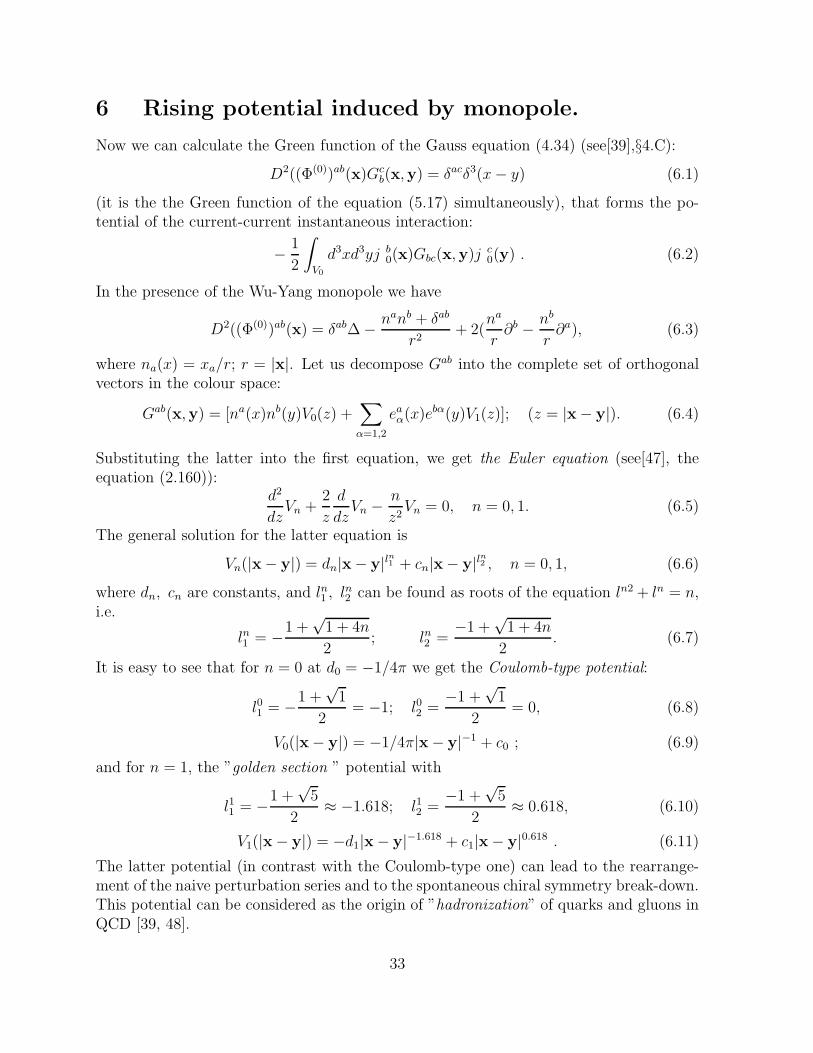


![arXiv:2109.11857v1 [nucl-th] 24 Sep 2021](https://static.documents.pub/doc/80x56/61808efaea4bc55678477184/arxiv210911857v1-nucl-th-24-sep-2021.jpg)


![arXiv:0907.2041v5 [hep-th] 3 Sep 2010](https://static.documents.pub/doc/80x56/6192914989a74b6caa645946/arxiv09072041v5-hep-th-3-sep-2010.jpg)


![arXiv:2109.09626v1 [nucl-th] 20 Sep 2021](https://static.documents.pub/doc/80x56/61848d1651ead761a870a381/arxiv210909626v1-nucl-th-20-sep-2021.jpg)